Abstract:

We use the worldline formalism to derive integral representations for three classes of amplitudes in scalar field theory: (i) the scalar propagator exchanging $N$ momenta with a scalar background field (ii) the “half-ladder” with $N$ rungs in $x$ - space (iii) the four-point ladder with $N$ rungs in $x$ - space as well as in (off-shell) momentum space. In each case we give a compact expression combining the $N!$ Feynman diagrams contributing to the amplitude. As our main application, we reconsider the well-known case of two massive scalars interacting through the exchange of a massless scalar. Applying asymptotic estimates and a saddle-point approximation to the $N$-rung ladder plus crossed ladder diagrams, we derive a semi-analytic approximation formula for the lowest bound state mass in this model.

1 Introduction

At about the same time when Feynman developed the modern approach to perturbative QED, based on Feynman diagrams, he also invented an alternative representation of the QED effective action or S-matrix in terms of first-quantized relativistic particle path integrals [1, 2]. For the simplest case, the one-loop effective action induced in scalar QED by an external Maxwell field $A$, this representation reads

$$\Gamma[A] = \int_{0}^{\infty}{dT\over T}\,{\rm e}^{-m^{2}T}{\displaystyle\int_{x(T)=x(0)}}{\cal D}x(\tau)\,e^{-\int_{0}^{T}d\tau[{1\over 4}\dot{x}^{2}+ie\dot{x}^{\mu}A_{\mu}(x(\tau))]}$$ (1.1)

Here $T$ denotes the proper-time of the scalar particle in the loop, $m$ its mass, and $\int_{x(T)=x(0)}{\cal D}x(\tau)$ a path integral over all closed loops in spacetime with fixed periodicity in the proper-time (we will use euclidean conventions throughout this paper). Photon amplitudes as usual are obtained by specializing the effective action to backgrounds involving a finite number of plane waves.

This formalism, which nowadays goes under various names, e.g. “Feynman-Schwinger representation”, “particle presentation”, “quantum mechanical path integral formalism”, “first-quantized formalism” or “worldline formalism” (which we will adopt here) has been studied by many authors, and extended to other field theories (see [3] for an extensive bibliography), but for several decades was considered as mainly of conceptual interest. However, partly as a consequence of developments in string theory [4], where first-quantized methods figure more prominently than in ordinary field theory, it has in recent years emerged also as a powerful practical tool for the computation of a wide variety of quantities in quantum field theory. This includes one-loop on-shell [5, 6, 7, 8] and off-shell [9, 10] photon/gluon amplitudes, one- and two-loop Euler-Heisenberg-Weisskopf Lagrangians [8, 11], heat-kernel coefficients [12, 13], Schwinger pair creation in constant [14] and non-constant fields [15, 16], Casimir energies [17], various types of anomalies (see [18] and refs. therein), QED/QCD bound states [19, 20, 21], heavy-quark condensates [22], and QED/QCD instantaneous Hamiltonians [23]. Extensions to curved space [24] and quantum gravity [25] have also been considered.

One of the interesting aspects of this approach is that often it combines into a single expression contributions from a large number of Feynman diagrams. For example, in the QED case it generally allows one to combine into one integral all contributions from Feynman diagrams which can be identified by letting photon legs slide along scalar/fermion loops or lines. Thus e.g. the well-known sum of six permuted diagrams for one-loop QED photon-photon scattering (see fig. 1) here naturally appears combined into a single integral [3].

Figure 1: Six permuted diagrams contributing to QED photon-photon scattering.

While in this case the summation involves graphs that differ only by permutations of the external legs, at higher loop orders the summation will generally involve topologically different diagrams; as an example, we show in fig. 2 the “quenched” contributions to the three-loop photon propagator.

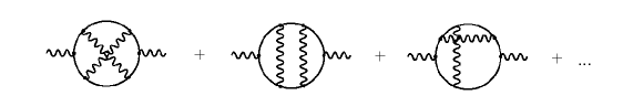
Figure 2: Diagrams contributing to the three loop QED photon propagator.

This property is particularly interesting in view of the fact that it is just this type of summation which in QED often leads to extensive cancellations, and to final results which are substantially simpler than intermediate ones (see, e.g., [26, 27]). More recently, similar cancellations have been found also for graviton amplitudes (see, e.g., [28]).

Although this property of the worldline formalism is well-known, and has been occasionally exploited [29, 30, 31] (see also [32]) a systematic study of its implications is presently still lacking. In this paper, we will initiate such a study for the simplest case of scalar field theory, considering two real scalar fields interacting through a cubic vertex. In this model, we will look at the following three classes of Green’s functions: the first one, depicted in fig. 3, is the $x$-space propagator for one scalar interacting with the second one through the exchange of $N$ given momenta.

Figure 3: Sum of diagrams contributing to the $N$ - propagator.

This object, to be called “$N$-propagator”, is given by a set of $N!$ simple tree-level graphs, and in section 2 we will use the worldline formalism to combine them into a single integral. We will also obtain the momentum-space version of this result.

The second class are the similarly looking $x$-space $N+2$ - point functions shown in fig 4, defined by a line connecting the points $x$ and $y$ and $N$ further points $z_{1},\ldots,z_{N}$ connecting to this line in an arbitrary order.

Figure 4: Sum of diagrams contributing to the half-ladder.

These “$N$-rung half-ladders” again form a set of $N!$ diagrams, and we will give a unifying integral representation in section 3. This class of diagrams is, apart from the first ($N=1$) one, which is just the well-known off-shell scalar triangle integral [33], already highly nontrivial; the four-point integral corresponding to $N=2$ figures prominently in $N=4$ SYM theory [34, 35, 36, 37] (it was called $f(x_{1},x_{2},x_{3},x_{4})$ in [34]) but is presently still not known in closed form. Here we will derive for it a novel two-parameter integral representation.

Finally, in section 4 we come to the class of ladder graphs, depicted in fig. 5, which we obtain by “gluing together” two “$N$-propagators”.

Figure 5: Sum of ladder and crossed-ladder contributions to the four-point function in $x$ - space.

Just as in the case of the $N$-propagators and half-ladders, one distinctive advantage of the worldline representation over the usual Feynman parameterization of this type of diagrams is the automatic inclusion of all possible ways of crossing the “rungs” of the ladders. Here again we will obtain such unifying representations in explicit form both in $x$-space and in momentum space.

Ladder graphs with a finite number $N$ of rungs play an important role for scattering processes in the high energy, large momentum transfer limit, see, e.g., ref. [38]. In this paper, we will concentrate on the case of infinite $N$, i.e., the sum over all ladder and crossed ladder graphs, which is of paramount importance for the bound state problem. In fact, our hope that a fresh look at these graphs from the perspective of the worldline formalism, usually refered to as the worldline representation in this context (see, e.g.,[39]), can give new insights in the bound state problem is the original motivation behind the present work.

It is our opinion that the bound state problem, in the sense of establishing an efficient and systematic formalism that would allow one to calculate the bound states and their properties for a given field theory, is one of the important open problems in quantum field theory, and that the fact that so little work is dedicated at present to this problem reflects its complexity rather than a lack of importance. It is evident, in fact, that the present-day description of (light) hadrons, which are intrinsically relativistic bound states of quarks and gluons, is not satisfactory from a theoretical standpoint. Not only a precise description of the effective interaction of quarks and gluons is missing, but also a convenient formalism for the calculation of the hadronic states once an appropriate description of the interaction is established.

This being said, a fully relativistic equation for the masses and structure of the bound states of two constituents has been established in quantum field theory a long time ago by Salpeter and Bethe [40, 41]. Unfortunately, the practical application of this equation suffers from all kinds of difficulties, see, e.g., ref. [42] for an early review. In particular, despite the fact that the equation is exact in principle, applications can hardly go beyond the ladder approximation to the equation which amounts to replacing the totality of diagrams contributing to the four-point function with the ladder graphs, excluding all crossed ladder graphs. The inclusion of the crossed ladder graphs, however, is essential for the consistency of the one-body limit where one of the constituents becomes infinitely heavy, and for maintaining gauge invariance (in gauge theories).

Alternatives to the Bethe-Salpeter equation have been devised that partially include the crossed ladder graphs, the best-known being the Blankenbecler-Sugar equation [43, 44], the Gross (or spectator) equation [45] and the equal-time equation [46]. In order to assess how well these so-called quasipotential equations are doing in incorporating the effects of the crossed-ladder graphs, and to establish some benchmark values for the relativistic bound state problem, Nieuwenhuis and Tjon [20] have numerically evaluated the path integrals of the worldline representation for the same scalar model field theory that we are considering here, thus including all ladder and crossed ladder graphs. The results, if the numerical evaluation is to be trusted, are not reassuring: while the predictions of the quasi-potential equations are closer to the numerical values for the lowest bound state mass than the solution of the Bethe-Salpeter equation, they still differ substantially from the worldline values (and from one another). On the other hand, the predictions of the quasipotential equations for the equal-time wave function of the lowest bound state are worse than the ones of the Bethe-Salpeter equation. Similar conclusions concerning the importance of crossed contributions were reached for the same model in the more extensive study by Savkli et al. [21]. Here both numerical and analytical methods were used in the evaluation of the worldline path integrals, and some results were obtained also for 1+1 dimensional Scalar QED.

In section 5, we will apply the worldline representation to the same scalar model field theory that was considered by Nieuwenhuis and Tjon, but we will derive concrete results for the mass of the lowest bound state for the case of a massless exchanged particle (along the “rungs” of the ladders), while Nieuwenhuis and Tjon took the mass of the exchanged particle to be $0{.}15$ times the mass of the constituents. Furthermore, we are interested in exploring how far one can get in an (approximate) analytical, rather than numerical, evaluation of the path integrals.

We should also like to mention that, particularly in the case of a massless exchanged particle, field theoretical perturbation theory can be applied in order to calculate corrections to the essentially nonrelativistic situation, as long as the coupling constant is sufficiently small. In this way, very precise predictions have been obtained for the case of positronium. For comparison, if one applies the Bethe-Salpeter equation in the ladder approximation to the scalar model field theory with a massless exchanged particle, known in this context as the Wick-Cutkosky model [47, 48], the bound state solutions tend to their nonrelativistic counterparts (the interaction of the constituents being described by a Coulomb potential) in the nonrelativistic limit of small coupling constant. However, already the first relativistic corrections (in an expansion in powers of the coupling constant) as predicted by the Bethe-Salpeter ladder approximation are considered unphysical [49, 50]. We will return to this issue in section 5.

Now let us define our model. We will work in the euclidean throughout in this paper. The action for our field theory with two scalars interacting through a cubic vertex is

$$S[\phi,\chi]=\int d^{D}x\,\bigg{(}{1\over 2}(\partial_{\mu}\phi)^{2}+{1\over 2}m^{2}\phi^{2}+{1\over 2}(\partial_{\mu}\chi)^{2}+{1\over 2}\mu^{2}\chi^{2}+{\lambda\over 2!}\phi^{2}\chi\bigg{)}\ .$$

(1.2)

Our most basic object of interest is the propagator for the $\phi$ - field in the background of the $\chi$ - field. The worldline representation of this propagator is (for a careful derivation see [51])

$$\langle 0|T\phi(x)\phi(y)|0\rangle_{(\chi)}=\int_{0}^{\infty}\!dT\,\mbox{e}^{-m^{2}T}\int_{{}_{x(0)=y}}^{{}^{\,x(T)=x}}\!\!\!\!\!\!\!\!\!\!\!\!{\cal D}x\ e^{-\int_{0}^{T}d\tau\,\big{[}{1\over 4}\dot{x}^{2}+\lambda\chi(x(\tau))\big{]}}\ .$$ (1.3)

Here the path integral runs over all trajectories in euclidean space that lead from $y$ to $x$ in the fixed proper-time $T$. From this propagator in the background field we can obtain the “$N$-propagator” for the $\phi$ - particle, describing its interaction with the $\chi$ - field through the interchange of $N$ quanta with four-momenta $k_{1},\ldots,k_{N}$. This simply requires specializing the background scalar field $\chi(x)$ to a sum of $N$ plane waves,

$$\chi(x)=\sum_{i=1}^{N}\mbox{e}^{ik_{i}\cdot x}$$ (1.4)

and picking the terms linear in each of the plane waves on the rhs of (1.3). For the $N$-propagator (1.3) induces the representation

$$\langle 0|T\phi(x)\phi(y)|0\rangle_{(N)} = (-\lambda)^{N}\int_{0}^{\infty}\!dT\,\mbox{e}^{-m^{2}T}\int_{0}^{T}d\tau_{1}\cdots\int_{0}^{T}d\tau_{N}$$

$$\times\int_{{}_{x(0)=y}}^{{}^{\,x(T)=x}}\!\!\!\!\!\!\!\!\!\!\!\!{\cal D}x\,\mbox{e}^{i\sum_{i=1}^{N}k_{i}\cdot x(\tau_{i})}\mbox{e}^{-\int_{0}^{T}d\tau\,{1\over 4}\dot{x}^{2}}\ .$$

The path integral is now of Gaussian type, so that it can be evaluated exactly using only the determinant and the inverse (“worldline Green function”) of the kinetic operator, which here is simply the second derivative operator in proper-time . In section 2 we will do this in detail. For the scalar field theory amplitudes considered in this paper, the resulting “worldline integrals” are related to standard Feynman parameter integrals in a straightforward way. However, they offer an advantage over Feynman parameter integrals in that they are valid independently of the ordering of the momenta $k_{1},\ldots,k_{N}$; the rhs of (LABEL:Nprop) contains already all $N!$ possibilities of attaching the $N$ momenta to the propagator, as shown in figure 3.

Although all the integrals considered in this paper are finite in four dimensions, we will work in a general dimension $D$, except in some of our more explicit calculations.

2 $N$-propagators

We proceed to the calculation of the Gaussian path integral (LABEL:Nprop). First, let us split $x^{\mu}(\tau)$ into a background part $x^{\mu}_{bg}(\tau)$, which encodes the boundary conditions, and a quantum part $q^{\mu}(\tau)$, which has zero Dirichlet boundary conditions at $\tau=0,T$,

$$x^{\mu}(\tau) = x^{\mu}_{bg}(\tau)+q^{\mu}(\tau)\,,$$

$$x^{\mu}_{bg}(\tau) = y^{\mu}+(x-y)^{\mu}\frac{\tau}{T}\,,$$

$$q^{\mu}(0)=q^{\mu}(T) = 0\,.$$

The propagator for $q^{\mu}(\tau)$ is the Green’s function for the second derivative operator on an interval of length $T$ with vanishing boundary conditions, which is [52, 6, 7]

$$\langle q^{\mu}(\tau)q^{\nu}(\sigma)\rangle = -2\delta^{\mu\nu}\Delta_{T}(\tau,\sigma)\,,$$

$$\Delta_{T}(\tau,\sigma) = \frac{\tau\sigma}{T}-\tau\theta(\sigma-\tau)-\sigma\theta(\tau-\sigma)$$

$$= \frac{\tau\sigma}{T}+\frac{|\tau-\sigma|}{2}-\frac{\tau+\sigma}{2}\,.$$

We note also the coincidence limit of this Green’s function,

$$\Delta_{T}(\tau,\tau)=\frac{\tau^{2}}{T}-\tau\ .$$

(2.3)

We will also need the free path integral normalization factor (see, e.g. [18])

$$\int_{{}_{q(0)=0}}^{{}^{\,q(T)=0}}\!\!\!\!\!\!\!\!\!\!\!\!{\cal D}q\,\mbox{e}^{-\int_{0}^{T}d\tau\,{1\over 4}\dot{q}^{2}}=\frac{1}{(4\pi T)^{D\over 2}}\,.$$ (2.4)

For the benefit of the reader unfamiliar with worldline path integrals, let us first consider the case $N=1$. From (LABEL:Nprop), (LABEL:split) and (2.4)

$$\langle 0|T\phi(x)\phi(y)|0\rangle_{{}_{\!(1)}}=\int_{0}^{\infty}\!{dT\over(4\pi T)^{D\over 2}}\,e^{-{(x-y)^{2}\over 4T}-m^{2}T}(-\lambda)\int_{0}^{T}d\tau\,e^{ik\cdot[y+(x-y)\frac{\tau}{T}]}\langle e^{ik\cdot q(\tau)}\rangle$$

(2.5)

with the Wick contraction

$$\langle e^{ik\cdot q(\tau)}\rangle=e^{k^{2}(\frac{\tau^{2}}{T}-\tau)}$$ (2.6)

by (2.3). Summarizing,

$$\langle 0|T\phi(x)\phi(y)|0\rangle_{{}_{\!(1)}}=\int_{0}^{\infty}\!{dT\over(4\pi T)^{D\over 2}}\,e^{-{(x-y)^{2}\over 4T}-m^{2}T}(-\lambda)\int_{0}^{T}d\tau\,\underbrace{e^{ik\cdot[y+(x-y)\frac{\tau}{T}]}}_{classical\ path}\,\underbrace{e^{-k^{2}(\tau-\frac{\tau^{2}}{T})}}_{Wick\ contr.}\,.$$

(2.7)

We Fourier transform in $x$ and $y$, rescale $\tau=Tu$, do the $T$ integral and obtain the product of two propagators in the Feynman parametrization

$$\langle\tilde{\phi}(p_{1})\tilde{\phi}(p_{2})\rangle_{{}_{\!(1)}}\!\! = \!\!(2\pi)^{D}\delta^{D}(p_{1}+p_{2}+k)(-\lambda)\int_{0}^{1}du\,\int_{0}^{\infty}dT\,T\,e^{-T[p_{1}^{2}+m^{2}+(k^{2}+2p_{1}\cdot k)u]}$$ (2.8)

$$= \!\!(2\pi)^{D}\delta^{D}(p_{1}+p_{2}+k)\,(-\lambda)\int_{0}^{1}du\,{\Gamma(2)\over[p_{1}^{2}+m^{2}+(k^{2}+2p_{1}\cdot k)u]^{2}}$$

$$= \!\!(2\pi)^{D}\delta^{D}(p_{1}+p_{2}+k)\,{1\over p_{1}^{2}+m^{2}}\,(-\lambda)\,{1\over(p_{1}+k)^{2}+m^{2}}\ .$$

Thus we have recovered the standard Feynman rule expression for the basic scalar vertex (fig. 6).

Figure 6: Scalar vertex

Proceeding directly to the $N$-point case, here (2.5) generalizes to

$$\langle 0|T\phi(x)\phi(y)|0\rangle_{{}_{\!(N)}} = \int_{0}^{\infty}\!{dT\over(4\pi T)^{D\over 2}}\,e^{-{(x-y)^{2}\over 4T}-m^{2}T}(-\lambda)^{N}\int_{0}^{T}d\tau_{1}\cdots\int_{0}^{T}d\tau_{N}$$

$$\times{\rm e}^{i\sum_{i}k_{i}\cdot\bigl{(}y+\frac{\tau_{i}}{T}(x-y)\bigr{)}}\langle e^{i\sum_{i=1}^{N}k_{i}\cdot q(\tau_{i})}\rangle\,.$$

After performing the Gaussian integration over $q^{\mu}(\tau)$ using the Green’s function (LABEL:defDelta), and a rescaling $\tau_{i}=Tu_{i}$, this becomes

$$\langle 0|T\phi(x)\phi(y)|0\rangle_{{}_{\!(N)}} = (-\lambda)^{N}\int_{0}^{\infty}\!{dT\over(4\pi T)^{D\over 2}}\,e^{-{(x-y)^{2}\over 4T}-m^{2}T}T^{N}\int_{0}^{1}du_{1}\cdot\cdot\int_{0}^{1}du_{N}\,$$

$$\times{\rm e}^{i\sum_{i}k_{i}\cdot\bigl{(}y+u_{i}(x-y)\bigr{)}}{\rm exp}\biggl{[}T\sum_{i,j=1}^{N}k_{i}\cdot k_{j}\Delta_{1}(u_{i},u_{j})\biggr{]}\,.$$

Fourier transformation of this representation yields, after an easy computation,

$$\langle\tilde{\phi}(p_{1})\tilde{\phi}(p_{2})\rangle_{{}_{\!(N)}} = (2\pi)^{D}\delta^{D}(p_{1}+p_{2}+\sum_{i}k_{i})(-\lambda)^{N}\int_{0}^{\infty}dT\int_{0}^{T}d\tau_{1}\cdot\cdot\int_{0}^{T}d\tau_{N}\,$$

$$\times{\rm exp}\biggl{\{}-T\Bigl{(}p_{1}^{2}+m^{2}\Bigr{)}-\sum_{i}(k_{i}^{2}+2p_{1}\cdot k_{i})\tau_{i}-\sum_{i<j}2k_{i}\cdot k_{j}D(\tau_{i},\tau_{j})\biggr{\}}$$

$$= (2\pi)^{D}\delta^{D}(p_{1}+p_{2}+\sum_{i}k_{i})(-\lambda)^{N}N!\int_{0}^{1}du_{1}\cdot\cdot\int_{0}^{1}du_{N}\,$$

$$\times\bigg{[}p_{1}^{2}+m^{2}+\sum_{i}(k_{i}^{2}+2p_{1}\cdot k_{i})u_{i}+\sum_{i<j}2k_{i}\cdot k_{j}D(u_{i},u_{j})\bigg{]}^{-N-1}\ .$$

where we have further defined

$$D(\tau_{i},\tau_{j}) := \tau_{i}\theta(\tau_{j}-\tau_{i})+\tau_{j}\theta(\tau_{i}-\tau_{j})\,.$$ (2.12)

Each of the $N!$ orderings of the $u_{1},..,u_{N}$ parameters along the worldline region $[0,1]$ identifies a range of integration. Each range of integration produces the product of the $(N+1)$ propagators where the momentum flows according to momentum conservation. This gives the total of $N!$ contributions corresponding to the various exchanges of the external lines carrying momentum $k^{\mu}_{i}$. The explicit proof is given in the appendix.

Our leitmotif in this paper is to find representations like (LABEL:orderNxspace) and (LABEL:orderNpspace) that unify the Feynman diagrams corresponding to different orderings. However, as an aside we wish to mention also that the contribution of any ordered sector to (LABEL:orderNxspace) can be recast in a form that is a finite-dimensional analogue of the initial path-integral (LABEL:Nprop). First, introducing the inverse of the $N\times N$ matrix $-\Delta_{ij}=-\Delta_{1}(u_{i},u_{j})$, as well as its determinant $|-\Delta|$, we can trivially rewrite the final exponential factor in (LABEL:orderNxspace) in terms of a Gaussian integral over auxiliary variables $\xi_{1},\ldots\xi_{N}$ as

$${\rm exp}\biggl{[}T\sum_{i,j=1}^{N}k_{i}\cdot k_{j}\Delta_{1}(u_{i},u_{j})\biggr{]} = \int d^{D}\xi_{1}\cdots\int d^{D}\xi_{N}\biggl{(}(4\pi T)^{N}|-\Delta|\biggr{)}^{-\frac{D}{2}}$$

$$\times\,{\rm exp}\biggl{[}-\frac{1}{4T}\sum_{i,j=1}^{N}(-\Delta^{-1})_{ij}\xi_{i}\cdot\xi_{j}+i\sum_{i=1}^{N}k_{i}\cdot\xi_{i}\biggr{]}\,.$$

It is sufficient to consider the standard ordering $1\geq u_{1}\geq u_{2}\geq\ldots\geq u_{N}\geq 0$. For this sector, it is straightforward to show inductively that $|-\Delta|$ and $(-\Delta^{-1})$ are given by

$$|-\Delta|=(1-u_{1})(u_{1}-u_{2})(u_{2}-u_{3})\cdots(u_{N-1}-u_{N})u_{N}$$ (2.14)

and

$$\small-\Delta^{-1}\!\!=\!\!\tiny\left(\begin{array}[]{ccccc}\frac{1}{1-u_{1}}+\frac{1}{u_{1}-u_{2}}&-\frac{1}{u_{1}-u_{2}}&0&0&0\\ -\frac{1}{u_{1}-u_{2}}&\frac{1}{u_{1}-u_{2}}+\frac{1}{u_{2}-u_{3}}&-\frac{1}{u_{2}-u_{3}}&0&0\\ \vdots&\vdots&\vdots&\vdots&\vdots\\ 0&0&-\frac{1}{u_{N-2}-u_{N-1}}&\frac{1}{u_{N-2}-u_{N-1}}+\frac{1}{u_{N-1}-u_{N}}&-\frac{1}{u_{N-1}-u_{N}}\\ 0&0&0&-\frac{1}{u_{N-1}-u_{N}}&\frac{1}{u_{N-1}-u_{N}}+\frac{1}{u_{N}}\end{array}\right)$$ (2.20)

(2.21)

Thus in the first term in the exponent in (LABEL:rewriteexp) we can rewrite

$$\sum_{i,j=1}^{N}(-\Delta^{-1})_{ij}\xi_{i}\cdot\xi_{j}=\frac{\xi_{1}^{2}}{1-u_{1}}+\sum_{i=1}^{N-1}\frac{(\xi_{i}-\xi_{i+1})^{2}}{u_{i}-u_{i+1}}+\frac{\xi_{N}^{2}}{u_{N}}$$ (2.22)

Using (2.22) in (LABEL:orderNxspace) and performing a linear shift

$$\xi_{i}\to\xi_{i}-y-u_{i}(x-y)$$ (2.23)

we get

$$\langle 0|T\phi(x)\phi(y)|0\rangle_{{}_{\!(N)}}^{(12\ldots N)}\!\! = \!\!(-\lambda)^{N}\int_{0}^{\infty}\!{dT\over(4\pi T)^{D\over 2}}\,e^{-m^{2}T}T^{N}\int_{0}^{1}du_{1}\int_{0}^{u_{1}}du_{2}\cdots\int_{0}^{u_{N-1}}du_{N}\,$$

$$\times\int d^{D}\xi_{1}\cdots\int d^{D}\xi_{N}\biggl{(}(4\pi T)^{N}|-\Delta|\biggr{)}^{-\frac{D}{2}}$$

$$\times{\rm exp}\Biggl{\{}-\frac{1}{4T}\biggl{[}\frac{(x-\xi_{1})^{2}}{1-u_{1}}+\sum_{i=1}^{N-1}\frac{(\xi_{i}-\xi_{i+1})^{2}}{u_{i}-u_{i+1}}+\frac{(\xi_{N}-y)^{2}}{u_{N}}\biggr{]}+i\sum_{i=1}^{N}k_{i}\cdot\xi_{i}\Biggr{\}}.$$

Here on the lhs the superscript $(12\ldots N)$ indicates the restriction to the standard ordering. Comparing with the original path integral (LABEL:Nprop) it will be observed that (LABEL:xirep) can be viewed as a restriction of this path integral to the finite-dimensional set of polygonal paths leading from $x$ to $y$, corresponding to the propagation of a particle that is free in between absorbing (or emitting), at proper-time $\tau_{i}=u_{i}T$ and the space-time point $\xi_{i}$, the momentum $k_{i}$. Alternatively, the representation (LABEL:xirep) of the $N$ - propagator can also be obtained using heat-kernel methods similar to the ones of [52]. Despite of its simplicity we have not been able to find this formula in the literature.

3 $N$-point half-ladders

We proceed to the set of half-ladder diagrams depicted in fig. 4. Those we will consider in $x$ - space only. They can be obtained from the $N$-propagators by replacing

$$e^{ik_{i}\cdot x(\tau_{i})}\to\int\frac{d^{D}k_{i}}{(2\pi)^{D}}\frac{e^{ik_{i}\cdot(x(\tau_{i})-z_{i})}}{k_{i}^{2}+\mu^{2}}$$ (3.1)

for $i=1,\ldots,N$. For $N=1$ we obtain, after this replacement, the usual Schwinger exponentiation

$$\frac{1}{k^{2}+\mu^{2}}=\int_{0}^{\infty}d\alpha\,{\rm e}^{-\alpha(k^{2}+\mu^{2})}$$ (3.2)

and the use of (2.7), the following representation for the lowest-order scalar $x$-space three-point function, with two propagators having mass $m$ and one having mass $\mu$:

$$\Gamma(x,y,z,m,\mu) = -\lambda\int_{0}^{\infty}\!{dT\over(4\pi T)^{D\over 2}}\,e^{-{(x-y)^{2}\over 4T}-m^{2}T}\int\frac{d^{D}k}{(2\pi)^{D}}\int_{0}^{\infty}d\alpha\,{\rm e}^{-(ik\cdot z+\alpha(k^{2}+\mu^{2}))}$$ (3.3)

$$\times\int_{0}^{T}d\tau\,e^{ik\cdot y}e^{ik\cdot(x-y)\frac{\tau}{T}}\,e^{-k^{2}(\tau-\frac{\tau^{2}}{T})}\,.$$

Performing the Gaussian $k$-integral and rescaling $\tau=Tu$ as well as $\alpha=T\hat{\alpha}$, we obtain

$$\Gamma(x,y,z,m,\mu) = -\frac{\lambda}{(4\pi)^{D}}\int_{0}^{\infty}\!\frac{dT}{T^{D-2}}\,e^{-{(x-y)^{2}\over 4T}-m^{2}T}\int_{0}^{\infty}d\hat{\alpha}\,e^{-\hat{\alpha}\mu^{2}T}$$ (3.4)

$$\times\int_{0}^{1}du\frac{1}{[\hat{\alpha}+u(1-u)]^{\frac{D}{2}}}e^{\frac{-(y-z+(x-y)u)^{2}}{4T(\hat{\alpha}+u(1-u))}}\,.$$

Now we specialize to the massless case, $m=\mu=0$. The $T$ - integral then becomes elementary, and one gets

$$\Gamma(x,y,z,0,0) = -\frac{\lambda}{(4\pi)^{D}}\Gamma(D-3)\int_{0}^{1}du\int_{0}^{\infty}d\hat{\alpha}$$

$$\times\frac{1}{[\hat{\alpha}+u(1-u)]^{\frac{D}{2}}}\frac{4^{D-3}}{\Bigl{[}(x-y)^{2}+\frac{[y-z+(x-y)u]^{2}}{\hat{\alpha}+u(1-u)}\Bigr{]}^{D-3}}\,.$$

Further simplification is possible if we now also assume $D=4$. This makes the $\hat{\alpha}$ - integral elementary, and results in

$$\Gamma(x,y,z,0,0) = -\frac{\lambda}{64\pi^{4}}\int_{0}^{1}\!du\frac{1}{uc+(1-u)b-u(1-u)a}\log\Bigl{[}\frac{uc+(1-u)b}{u(1-u)a}\Bigr{]}$$

where we have now abbreviated

$$(x-y)^{2}=a\,,\hskip 20.0pt(y-z)^{2}=b\,,\hskip 20.0pt(x-z)^{2}=c\,.$$ (3.6)

The $u$ - integral can be reduced to the standard integral

$$\int du\frac{\ln(Au+B)}{u-C} = \ln(Au+B)\ln\Bigl{(}1-\frac{Au+B}{AC+B}\Bigr{)}+{\rm Li}_{2}\Bigl{(}\frac{Au+B}{AC+B}\Bigr{)}\,.$$

The final result is then easy to identify with the well-known representation of the massless triangle function due to Ussyukina and Davydychev [33],

$$\Gamma(x,y,z,0,0)=-\frac{\lambda}{64\pi^{4}}\frac{1}{a}\Phi^{(1)}\Bigl{(}\frac{b}{a},\frac{c}{a}\Bigr{)}$$ (3.8)

where

$$\Phi^{(1)}(x,y) := {1\over\Lambda}\Biggl{\{}2\Bigl{(}{\rm Li}_{2}(-\rho x)+{\rm Li}_{2}(-\rho y)\Bigr{)}+\ln{y\over x}\ln{{1+\rho y}\over{1+\rho x}}+\ln(\rho x)\ln(\rho y)+{\pi^{2}\over 3}\Biggr{\}}$$

with

$$\Lambda := \sqrt{(1-x-y)^{2}-4xy},$$

$$\rho := 2(1-x-y+\Lambda)^{-1}.$$

After this warm-up, we proceed to the much more challenging $N=2$ case. Eq. (3.3) generalizes straightforwardly to

$$\Gamma(x,y,z_{1},z_{2},m,\mu) = (-\lambda)^{2}\int^{\infty}_{0}\frac{dT\,T^{2}}{(4\pi T)^{D/2}}e^{-\frac{(x-y)^{2}}{4T}-m^{2}T}\int\frac{d^{D}k_{1}}{(2\pi)^{D}}\int\frac{d^{D}k_{2}}{(2\pi)^{D}}\,e^{-i(k_{1}\cdot z_{1}+k_{2}\cdot z_{2})}$$

$$\times\int_{0}^{\infty}d\alpha_{1}e^{-\alpha_{1}(k_{1}^{2}+\mu^{2})}\int_{0}^{\infty}d\alpha_{2}\,e^{-\alpha_{2}(k_{2}^{2}+\mu^{2})}\int^{1}_{0}du_{1}\int^{1}_{0}du_{2}$$

$$\times e^{ik_{1}\cdot[y+(x-y)u_{1}]}e^{ik_{2}\cdot[y+(x-y)u_{2}]}e^{T\bigr{[}k_{1}^{2}\bigtriangleup_{1}(u_{1},u_{1})+k_{2}^{2}\bigtriangleup_{1}(u_{2},u_{2})+2k_{1}\cdot k_{2}\bigtriangleup_{1}(u_{1},u_{2})\bigr{]}}\,.$$

Here we have already rescaled $\tau_{i}=Tu_{i}$, $i=1,2$. The ordered sector $u_{1}<u_{2}$ of this integral corresponds to the first diagram shown in fig. 4 (for $N=2$), the sector $u_{1}>u_{2}$ to the second one.

As before, we first do the Gaussian $k_{1,2}$ - integrals, and obtain (in the following we abbreviate $\bigtriangleup_{1}(u_{i},u_{j})$ by $\bigtriangleup_{ij}$)

$$\Gamma(x,y,z_{1},z_{2},m,\mu) = \frac{\lambda^{2}}{(4\pi)^{D}}\int^{\infty}_{0}\frac{dT\,T^{2}}{(4\pi T)^{D/2}}e^{-\frac{(x-y)^{2}}{4T}-m^{2}T}\int^{1}_{0}du_{1}du_{2}\int_{0}^{\infty}d\alpha_{1}d\alpha_{2}e^{-(\alpha_{1}+\alpha_{2})\mu^{2}}$$

$$\times\frac{{\rm exp}\Bigl{\{}-\frac{(\alpha_{1}-T\bigtriangleup_{11})\beta_{2}^{2}+(\alpha_{2}-T\bigtriangleup_{22})\beta_{1}^{2}+2T\bigtriangleup_{12}\beta_{1}\cdot\beta_{2}}{4\bigl{[}(\alpha_{1}-T\bigtriangleup_{11})(\alpha_{2}-T\bigtriangleup_{22})-T^{2}\bigtriangleup_{12}^{2}\bigr{]}}\Bigr{\}}}{\Bigl{[}(\alpha_{1}-T\bigtriangleup_{11})(\alpha_{2}-T\bigtriangleup_{22})-T^{2}\bigtriangleup_{12}^{2}\Bigr{]}^{\frac{D}{2}}}\,$$

where we have defined

$$\beta_{i}:=y-z_{i}+u_{i}(x-y)\,.$$ (3.13)

Specializing to the massless case $m=\mu=0$, and changing from $\alpha_{i}$ to $\hat{\alpha}_{i}$ via

$$\alpha_{i}=T(\hat{\alpha}_{i}+\bigtriangleup_{ii}),\quad i=1,2,$$ (3.14)

we can do the $T$ - integral. This leads to

$$\Gamma(x,y,z_{1},z_{2},0,0) = \frac{\lambda^{2}}{(4\pi)^{\frac{3}{2}D}}\Gamma\Bigl{(}1+\frac{3}{2}(D-4)\Bigr{)}\int^{1}_{0}du_{1}du_{2}\int_{-\bigtriangleup_{11}}^{\infty}d\hat{\alpha}_{1}\int_{-\bigtriangleup_{22}}^{\infty}d\hat{\alpha}_{2}$$

$$\times\frac{1}{\Bigl{[}\hat{\alpha}_{1}\hat{\alpha}_{2}-\Delta_{12}^{2}\Bigr{]}^{\frac{D}{2}}}\Biggl{[}\frac{4}{(x-y)^{2}+\frac{\hat{\alpha}_{1}\beta_{2}^{2}+\hat{\alpha}_{2}\beta_{1}^{2}+2\Delta_{12}\beta_{1}\cdot\beta_{2}}{\hat{\alpha}_{1}\hat{\alpha}_{2}-\Delta_{12}^{2}}}\Biggr{]}^{1+\frac{3}{2}(D-4)}$$

Setting $D=4$, this becomes

$$\Gamma(x,y,z_{1},z_{2},0,0) = \frac{4\lambda^{2}}{(4\pi)^{6}}\int^{1}_{0}du_{1}du_{2}\int_{-\bigtriangleup_{11}}^{\infty}d\hat{\alpha}_{1}\int_{-\bigtriangleup_{22}}^{\infty}d\hat{\alpha}_{2}$$

$$\times\frac{1}{\Bigl{[}\hat{\alpha}_{1}\hat{\alpha}_{2}-\Delta_{12}^{2}\Bigr{]}\Bigl{[}(x-y)^{2}(\hat{\alpha}_{1}\hat{\alpha}_{2}-\Delta_{12}^{2})+\hat{\alpha}_{1}\beta_{2}^{2}+\hat{\alpha}_{2}\beta_{1}^{2}+2\Delta_{12}\beta_{1}\cdot\beta_{2}\Bigr{]}}\,.$$

Performing the $\hat{\alpha}_{1}$ - integral, which is elementary, we find

$$\Gamma(x,y,z_{1},z_{2},0,0) = \frac{4\lambda^{2}}{(4\pi)^{6}}\int^{1}_{0}du_{1}du_{2}\int_{-\bigtriangleup_{22}}^{\infty}d\hat{\alpha}_{2}$$

$$\times\frac{\ln\Biggl{\{}\frac{\hat{\alpha}_{2}\bigl{[}\hat{\alpha}_{2}(\beta_{1}^{2}-\Delta_{11}(x-y)^{2})+2\Delta_{12}\beta_{1}\cdot\beta_{2}-\Delta_{11}\beta_{2}^{2}-\Delta_{12}^{2}(x-y)^{2}\bigr{]}}{(\hat{\alpha}_{2}(-\Delta_{11})-\Delta_{12}^{2})(\hat{\alpha}_{2}(x-y)^{2}+\beta_{2}^{2})}\Biggr{\}}}{(\hat{\alpha}_{2}\beta_{1}+\Delta_{12}\beta_{2})^{2}}\,.$$

The $\hat{\alpha}_{2}$ - integral is still a straightforward one. Introducing the zeroes $\hat{\alpha}_{\pm}$ of the quadratic form in the denominator,

$$\hat{\alpha}_{\pm}:=-\frac{\Delta_{12}}{\beta_{1}^{2}}\Bigl{[}\beta_{1}\cdot\beta_{2}\pm i\sqrt{\beta_{1}^{2}\beta_{2}^{2}-(\beta_{1}\cdot\beta_{2})^{2}}\Bigr{]}$$

(3.18)

we can write the result as

$$\Gamma(x,y,z_{1},z_{2},0,0) = \frac{4\lambda^{2}}{(4\pi)^{6}}\int^{1}_{0}du_{1}du_{2}\frac{1}{(\hat{\alpha}_{+}-\hat{\alpha}_{-})\beta_{1}^{2}}\biggl{[}\ln\Biggl{(}\frac{-\Delta_{11}a+\beta_{1}^{2}}{-\Delta_{11}a}\Biggr{)}\ln\Biggl{(}\frac{-\Delta_{22}-\hat{\alpha}_{-}}{-\Delta_{22}-\hat{\alpha}_{+}}\Biggr{)}$$

$$+I(0)+I\biggl{(}\frac{2\Delta_{12}\beta_{1}\cdot\beta_{2}-\Delta_{11}\beta_{2}^{2}-\Delta_{12}^{2}a}{\beta_{1}^{2}-\Delta_{11}a}\biggr{)}-I\Bigl{(}\frac{\Delta_{12}^{2}}{\Delta_{11}}\Bigr{)}-I\Bigl{(}\frac{\beta_{2}^{2}}{a}\Bigr{)}\biggr{]}$$

where

$$I(A) := (\hat{\alpha}_{+}-\hat{\alpha}_{-})\int_{-\bigtriangleup_{22}}^{\infty}d\hat{\alpha}_{2}\frac{\ln(\hat{\alpha}_{2}+A)}{(\hat{\alpha}_{2}-\hat{\alpha}_{+})(\hat{\alpha}_{2}-\hat{\alpha}_{-})}$$ (3.20)

$$= \biggl{\{}{\rm Li}_{2}\Bigl{(}\frac{A-\Delta_{22}}{A+\hat{\alpha}_{-}}\Bigr{)}+\ln(A-\Delta_{22})\ln\Bigl{(}\frac{\hat{\alpha}_{-}+\Delta_{22}}{\hat{\alpha}_{-}+A}\Bigr{)}$$

$$+\frac{1}{2}\ln^{2}\Bigl{(}-\frac{1}{A+\hat{\alpha}_{-}}\Bigr{)}\biggr{\}}-(\hat{\alpha}_{-}\to\hat{\alpha}_{+})$$

and we have abbreviated $a:(x-y)^{2}$ as before. To rewrite the new integrand completely in terms of the external Lorentz invariants, we further introduce

$$b_{i} := (x-z_{i})^{2}\,,$$

$$c_{i} := (y-z_{i})^{2}\,,$$

$$d := (z_{1}-z_{2})^{2}\,.$$ (3.21)

In terms of these variables,

$$\beta_{i}^{2} = u_{i}b_{i}+(1-u_{i})c_{i}-u_{i}(1-u_{i})a\,,$$

$$2\beta_{1}\cdot\beta_{2} = (2u_{1}u_{2}-u_{1}-u_{2})a+u_{2}b_{1}+u_{1}b_{2}+(1-u_{2})c_{1}+(1-u_{1})c_{2}-d\,.$$

Although we are not able to perform the remaining two integrals analytically, the representation (LABEL:Gammafourmassless2) is still more explicit than other representations available for this integral which, as was mentioned in the introduction, plays an important role in SYM theory [34, 35, 36, 37].

For the general $N$-rung case, the formulas (3.3), (LABEL:starting2) generalize immediately to

$$\Gamma(x,y,z_{1},z_{2},\ldots,z_{N}) = (-\lambda)^{N}\int^{\infty}_{0}\frac{dT\,T^{N}}{(4\pi T)^{D/2}}e^{-\frac{(x-y)^{2}}{4T}-m^{2}T}\int\frac{d^{D}k_{1}}{(2\pi)^{D}}\cdots\frac{d^{D}k_{N}}{(2\pi)^{D}}\,e^{-i\sum_{i=1}k_{i}\cdot z_{i}}$$ (3.23)

$$\times\int d\alpha_{1}\cdots d\alpha_{N}e^{-\sum_{i=1}^{N}\alpha_{i}(k_{i}^{2}+\mu^{2})}\int du_{1}\ldots du_{N}e^{i\sum_{i=1}^{N}k_{i}\cdot(y+(x-y)u_{i})}$$

$$\times{\rm exp}\Bigl{[}T\sum_{i,j=1}^{N}\Delta_{ij}k_{i}\cdot k_{j}\Bigr{]}\,.$$

The formulas (3.4), (LABEL:Gammafourkdone) generalize to

$$\Gamma(x,y,z_{1},z_{2},\ldots,z_{N}) = \frac{(-\lambda)^{N}}{(4\pi)^{N\frac{D}{2}}}\int^{\infty}_{0}\frac{dT\,T^{N(2-D/2)}}{(4\pi T)^{D/2}}e^{-\frac{(x-y)^{2}}{4T}-m^{2}T}\int_{0}^{1}du_{1}\cdots du_{N}$$

$$\times\int_{0}^{\infty}d\hat{\alpha}_{1}\cdots d\hat{\alpha}_{N}e^{-\sum_{i=1}^{N}\hat{\alpha}_{i}\mu^{2}T}\frac{1}{(\det H_{N})^{\frac{D}{2}}}e^{-\frac{1}{4T}\vec{b}_{N}^{T}H_{N}^{-1}\vec{b}_{N}}\,.$$

Here $H_{N}$ is the symmetric $N\times N$ matrix with entries

$$H_{Nii} = \hat{\alpha}_{i}-\Delta_{ii}\,,$$

$$H_{Nij} = -\Delta_{ij}\quad(i\neq j)\,,$$

and $\vec{b}_{N}=(\beta_{1},\ldots,\beta_{N})$ with $\beta_{i}$ as defined in (3.13).

Finally, also the massless four-dimensional formula (LABEL:Gammafourmassless) can still be generalized to arbitrary $N$, in the form

$$\Gamma(x,y,z_{1},z_{2},\ldots,z_{N},0,0) = \frac{4(-\lambda)^{N}}{(4\pi)^{2(N+1)}}\int^{1}_{0}du_{1}\cdots du_{N}\int_{0}^{\infty}d\hat{\alpha}_{1}\cdots\hat{\alpha}_{N}$$

$$\times\frac{1}{(\det H_{N})^{2}\Bigl{[}(x-y)^{2}+\vec{b}_{N}^{T}H_{N}^{-1}\vec{b}_{N}\Bigr{]}}\,.$$

It seems not to be possible, though, to do all the $\hat{\alpha}_{i}$ - integrals in closed form for general $N$.

4 $N$-rung ladders

We will now come to our main purpose, namely to use the representations obtained for the $N$-propagators in section 2 for constructing the sum of all ladder and crossed-ladder graphs with $N$ rungs (simply called “$N$-ladders” in the following) in our scalar Yukawa theory (1.2).

Let us start with the graphs in momentum space. Starting with the product of two copies of (LABEL:orderNpspace), identifying $k_{i}$ of one $N$ - propagator with $-k_{i}$ of the second one, and inserting the connecting propagator integrals

$$\int\frac{dk_{1}}{(2\pi)^{D}}\frac{1}{k_{1}^{2}+\mu^{2}}\ldots\int\frac{dk_{N}}{(2\pi)^{D}}\frac{1}{k_{N}^{2}+\mu^{2}}$$

produces precisely $N!$ times the $N$-ladder graphs (the momentum space versions of the graphs shown in fig. 5; replace $y,{\bar{y}},x,{\bar{x}}$ by (incoming) momenta $(p_{1},p_{2},q_{1},q_{2})$ there). We obtain the following integral representation for the sum of these graphs:

$$\langle\tilde{\phi}(q_{1})\tilde{\phi}(q_{2})\tilde{\phi}(p_{1})\tilde{\phi}(p_{2})\rangle_{{}_{\!(N)}} = (2\pi)^{D}\delta^{D}(p_{1}+p_{2}+q_{1}+q_{2})\frac{\lambda^{2N}}{N!}\int_{0}^{\infty}dS\int_{0}^{\infty}dT\,{\rm e}^{-m^{2}(S+T)}$$

$$\times\int_{0}^{S}d\sigma_{1}\cdot\cdot\int_{0}^{S}d\sigma_{N}\,\int_{0}^{T}d\tau_{1}\cdot\cdot\int_{0}^{T}d\tau_{N}\,$$

$$\times\int\frac{dk_{1}}{(2\pi)^{D}}\frac{1}{k_{1}^{2}+\mu^{2}}\ldots\int\frac{dk_{N}}{(2\pi)^{D}}\frac{1}{k_{N}^{2}+\mu^{2}}(2\pi)^{D}\delta^{D}(p_{1}+p_{2}+\sum_{i}k_{i})$$

$$\times{\rm exp}\biggl{\{}-Sp_{1}^{2}-\sum_{i}(k_{i}^{2}+2p_{1}\cdot k_{i})\sigma_{i}-\sum_{i<j}2k_{i}\cdot k_{j}D(\sigma_{i},\sigma_{j})\biggr{\}}$$

$$\times{\rm exp}\biggl{\{}-Tq_{1}^{2}-\sum_{i}(k_{i}^{2}-2q_{1}\cdot k_{i})\tau_{i}-\sum_{i<j}2k_{i}\cdot k_{j}D(\tau_{i},\tau_{j})\biggr{\}}\,.$$

Next, we introduce Schwinger parameters $\alpha_{1},\ldots,\alpha_{N}$ to exponentiate the “rung” propagators, and we also (re-)exponentiate the second $\delta$ - function,

$$(2\pi)^{D}\delta^{D}\bigl{(}p_{1}+p_{2}+\sum_{i}k_{i}\bigr{)} = \int dv\,{\rm e}^{iv\cdot\bigl{(}p_{1}+p_{2}+\sum_{i}k_{i}\bigr{)}}\,.$$ (4.2)

The $k_{i}$ - integrals are now Gaussian, and performing them involves only the inverse and the determinant of the symmetric $N\times N$ - matrix $A_{N}$ with entries

$$A_{Nii} = \sigma_{i}+\tau_{i}+\alpha_{i}\,,$$

$$A_{Nij} = D(\sigma_{i},\sigma_{j})+D(\tau_{i},\tau_{j})\quad(i\neq j)\,.$$

The $v$ - integral then also becomes Gaussian. Doing it one is left with the following integral representation for the $N$ - ladder (henceforth we will omit the global $\delta$ function factor $(2\pi)^{D}\delta^{D}(p_{1}+p_{2}+q_{1}+q_{2})$):

$$\langle\tilde{\phi}(q_{1})\tilde{\phi}(q_{2})\tilde{\phi}(p_{1})\tilde{\phi}(p_{2})\rangle_{{}_{\!(N)}} = \frac{1}{(4\pi)^{(N-1)\frac{D}{2}}}\frac{\lambda^{2N}}{N!}\int_{0}^{\infty}dS\int_{0}^{\infty}dT\,{\rm e}^{-m^{2}(S+T)}$$

$$\times\int_{0}^{S}d\sigma_{1}\cdot\cdot\int_{0}^{T}d\tau_{N}\,\int_{0}^{\infty}d\alpha_{1}\cdot\cdot\int_{0}^{\infty}d\alpha_{N}\,\frac{{\rm e}^{-\mu^{2}\sum_{i}\alpha_{i}}}{(a_{N}\,{\rm det}{A_{N}})^{\frac{D}{2}}}$$

$$\times{\rm exp}\biggl{\{}-Sp_{1}^{2}-Tq_{1}^{2}-\frac{b_{N}^{2}}{a_{N}}+(p_{1}\vec{\sigma}-q_{1}\vec{\tau})\cdot A_{N}^{-1}\cdot(p_{1}\vec{\sigma}-q_{1}\vec{\tau})\biggr{\}}\,.$$

Here we have further defined

$$a_{N} := \vec{1}\cdot A^{-1}\cdot\vec{1}\,,$$

$$b_{N} := p_{1}+p_{2}-\vec{1}\cdot A_{N}^{-1}\cdot\vec{\sigma}\,p_{1}+\vec{1}\cdot A_{N}^{-1}\cdot\vec{\tau}\,q_{1}\,,$$

with $\vec{1}:=(1,\ldots,1)$, $\vec{\sigma}:=(\sigma_{1},\ldots,\sigma_{N})$ etc. It is understood that the matrix $A_{N}$ acts trivially on Lorentz indices. Note that (LABEL:ladderpfin) is still valid in $D$ dimensions.

Fourier transforming (LABEL:ladderpfin) we obtain the corresponding amplitude in $x$ - space in the form

$$\langle\phi_{q}(x)\phi_{q}(\bar{x})\phi_{q}(y)\phi_{q}(\bar{y})\rangle_{{}_{\!(N)}} = \frac{1}{(4\pi)^{(N+2)\frac{D}{2}}}\frac{\lambda^{2N}}{N!}\int_{0}^{\infty}dS\int_{0}^{\infty}dT\,{\rm e}^{-m^{2}(S+T)}$$

$$\times\int_{0}^{S}d\sigma_{1}\cdot\cdot\int_{0}^{T}d\tau_{N}\,\int_{0}^{\infty}d\alpha_{1}\cdot\cdot\int_{0}^{\infty}d\alpha_{N}\,\frac{{\rm e}^{-\mu^{2}\sum_{i}\alpha_{i}}}{({\rm det}L{\rm det}{A_{N}})^{\frac{D}{2}}}$$

$$\times{\rm exp}\biggl{\{}-\frac{1}{4}\Bigl{[}a_{N}(y-\bar{y})^{2}+(w,\bar{w})L^{-1}(w,\bar{w})\Bigr{]}\biggr{\}}$$

where

$$L := \left(\begin{array}[]{cc}S-\vec{\sigma}A_{N}^{-1}\vec{\sigma}&\vec{\sigma}A_{N}^{-1}\vec{\tau}\\ \vec{\sigma}A_{N}^{-1}\vec{\tau}&T-\vec{\tau}A_{N}^{-1}\vec{\tau}\\ \end{array}\right)\,,$$ (4.9)

$$w := x-y+\vec{1}A_{N}^{-1}\vec{\sigma}\,(y-\bar{y})\,,$$

$$\bar{w} := \bar{x}-\bar{y}-\vec{1}A_{N}^{-1}\vec{\tau}\,(y-\bar{y})\,.$$

Starting instead directly from (LABEL:orderNxspace), one finds the alternative, very compact form

$$\langle\phi_{q}(x)\phi_{q}(\bar{x})\phi_{q}(y)\phi_{q}(\bar{y})\rangle_{{}_{\!(N)}} = \frac{1}{(4\pi)^{(N+2)\frac{D}{2}}}\frac{\lambda^{2N}}{N!}\int_{0}^{\infty}dS\int_{0}^{\infty}dT\,{\rm e}^{-m^{2}(S+T)-\frac{(x-y)^{2}}{4S}-\frac{(\bar{x}-\bar{y})^{2}}{4T}}$$

$$\times\int_{0}^{S}d\sigma_{1}\cdot\cdot\int_{0}^{T}d\tau_{N}\,\int_{0}^{\infty}d\alpha_{1}\cdot\cdot\int_{0}^{\infty}d\alpha_{N}\,\frac{{\rm e}^{-\mu^{2}\sum_{i}\alpha_{i}-\frac{1}{4}\vec{r}M_{N}^{-1}\vec{r}}}{(ST{\rm det}{M_{N}})^{\frac{D}{2}}}$$

where $M_{N}$ is the symmetric $N\times N$ matrix

$$M_{Nij} := \delta_{ij}\alpha_{i}-\Delta_{S}(\sigma_{i},\sigma_{j})-\Delta_{T}(\tau_{i},\tau_{j})$$

and

$$\vec{r} := (y-\bar{y})\vec{1}+\frac{x-y}{S}\vec{\sigma}-\frac{(\bar{x}-\bar{y})}{T}\vec{\tau}\,.$$ (4.13)

We note that the two $x$-space representations (LABEL:ladderxfin1),(LABEL:ladderxfin2) can be related by

$$M_{N} = A_{N}-\frac{\vec{\sigma}\otimes\vec{\sigma}}{S}-\frac{\vec{\tau}\otimes\vec{\tau}}{T}\,,$$

$$M_{N}^{-1} = A_{N}^{-1}+L_{11}^{-1}A_{N}^{-1}\cdot\vec{\sigma}\,\vec{\sigma}\cdot A_{N}^{-1}-L_{12}^{-1}A_{N}^{-1}\cdot\vec{\sigma}\,\vec{\tau}\cdot A_{N}^{-1}-L_{21}^{-1}A_{N}^{-1}\cdot\vec{\tau}\,\vec{\sigma}\cdot A_{N}^{-1}$$

$$+L_{22}^{-1}A_{N}^{-1}\cdot\vec{\tau}\,\vec{\tau}\cdot A_{N}^{-1}\,,$$

which also implies that

$$ST{\rm det}M_{N} = {\rm det}L\,{\rm det}A_{N}\,.$$ (4.15)

5 An application: lowest bound state mass from scalar ladders

We proceed to the simplest possible application of our formulas for the ladder graphs to the physics of bound states, which is the extraction of the lowest bound state mass. Following [20], this can be done by considering the limit of large timelike separation $t\to\infty$, where

$$t = \frac{1}{2}(x_{4}+\bar{x}_{4}-y_{4}-\bar{y}_{4})\,.$$ (5.1)

Denoting the four – point Green’s function in the ladder approximation by $G$,

$$G = \sum_{N=0}^{\infty}G_{N}=\sum_{N=0}^{\infty}\langle\phi(x)\phi(\bar{x})\phi(y)\phi(\bar{y})\rangle_{{}_{\!(N)}}$$ (5.2)

one has

$$G \stackrel{{\scriptstyle t\to\infty}}{{\simeq}} c_{0}\,{\rm e}^{-m_{0}t}$$ (5.3)

where $m_{0}$ is the lowest bound state mass. We can set $D=4$, since no regularization will be required. Since we are not interested in the wave function of the bound state at present, we can simplify the formula for $G$ by setting

$$x=\bar{x},\quad y=\bar{y}$$ (5.4)

so that $t=x_{4}-y_{4}=\bar{x}_{4}-\bar{y}_{4}$. Further, since the limit $t\to\infty$ is taken at finite spatial displacement, in this limit we can effectively set

$$t^{2} = (x-y)^{2}=(\bar{x}-\bar{y})^{2}\,.$$ (5.5)

Using these relations in eqs. (LABEL:ladderxfin2), introducing the dimensionless time parameter

$$\hat{t}:=\frac{m}{2}t$$ (5.6)

as well as the effective coupling constant

$$g := \frac{\lambda^{2}}{(4\pi)^{2}m^{2}}\,,$$ (5.7)

rescaling $S,T,\alpha_{i}$ all by a factor $\hat{t}/m^{2}$, and changing variables from $\sigma_{i},\tau_{i}$ to $u_{i},v_{i}$ through

$$\sigma_{i}=S\frac{\hat{t}}{m^{2}}u_{i},\quad\tau_{i}=T\frac{\hat{t}}{m^{2}}v_{i}\,,$$ (5.8)

we get our following “master formula”,

$$G_{N} = \frac{m^{4}}{(4\pi)^{4}\hat{t}^{2}}\frac{(\hat{t}g)^{N}}{N!}\int_{0}^{\infty}dS\,S^{N-2}\int_{0}^{\infty}dT\,T^{N-2}$$

$$\times\int_{0}^{1}du_{1}\cdot\cdot\int_{0}^{1}dv_{N}\,\int_{0}^{\infty}d\alpha_{1}\cdot\cdot\int_{0}^{\infty}d\alpha_{N}\,\frac{1}{({\rm det}{\hat{M}_{N}})^{2}}$$

$$\times{\rm exp}\biggl{\{}-\hat{t}\biggl{[}S+T+\frac{1}{S}+\frac{1}{T}+\frac{\mu^{2}}{m^{2}}\sum_{i}\alpha_{i}+(\vec{u}-\vec{v})\hat{M}_{N}^{-1}(\vec{u}-\vec{v})\biggr{]}\biggr{\}}$$

where now

$$\hat{M}_{Nij} := \delta_{ij}\alpha_{i}-S\Delta_{1}(u_{i},u_{j})-T\Delta_{1}(v_{i},v_{j})\,.$$

We remark that in [31], inspired by Feynman’s famous treatment of the polaron problem [53], Barro-Bergflödt, Rosenfelder and Stingl have approximated the action in the worldline or Feynman-Schwinger representation of the four-point Green’s function $G$ (but including the self-energy and vertex corrections) by a quadratic trial action, in order to obtain an approximate value for the mass of the lowest-lying bound state. Here, we will use the large $\hat{t}$ limit to eliminate, at fixed $S,T,\alpha_{i},u_{i}$, the $v_{i}$ integrals by a Gaussian approximation around the point $\vec{v}=\vec{u}$. For the validity of this approximation, it is essential that the matrix $\hat{M}_{N}$ be positive semidefinite, which we have checked numerically for various values of $N$. The Gaussian approximation results in

$$G_{N} = \frac{m^{4}}{(4\pi)^{4}\hat{t}^{2}}\frac{(\pi\hat{t}g^{2})^{N/2}}{N!}\int_{0}^{\infty}dS\,S^{N-2}\int_{0}^{\infty}dT\,T^{N-2}$$

$$\times\int_{0}^{1}du_{1}\cdot\cdot\int_{0}^{1}du_{N}\,\int_{0}^{\infty}d\alpha_{1}\cdot\cdot\int_{0}^{\infty}d\alpha_{N}\,\frac{1}{({\rm det}{\bar{M}_{N}})^{3/2}}$$

$$\times{\rm exp}\biggl{\{}-\hat{t}\biggl{[}S+T+\frac{1}{S}+\frac{1}{T}+\frac{\mu^{2}}{m^{2}}\sum_{i}\alpha_{i}\biggr{]}\biggr{\}}$$

where now

$$\bar{M}_{Nij} := \delta_{ij}\alpha_{i}-(S+T)\Delta_{1}(u_{i},u_{j})\,.$$

After a further rescaling

$$\alpha_{i}\equiv(S+T)\hat{\alpha}_{i}$$ (5.13)

and summation over $N$, we obtain the following representation for the full Green’s function:

$$G = \frac{m^{4}}{(4\pi)^{4}\hat{t}^{2}}\int_{0}^{\infty}\frac{dS}{S^{2}}\int_{0}^{\infty}\frac{dT}{T^{2}}\,{\rm exp}\biggl{\{}-\hat{t}\biggl{[}S+T+\frac{1}{S}+\frac{1}{T}\biggr{]}\biggr{\}}$$

$$\times\sum_{N=1}^{\infty}\frac{(\pi\hat{t}g^{2})^{N/2}}{N!}\biggl{[}\frac{ST}{(S+T)^{1/2}}\biggr{]}^{N}c_{N}\Bigl{(}\hat{t}(S+T)\mu^{2}/m^{2}\Bigr{)}$$

where

$$c_{N}(x):=\int_{0}^{1}du_{1}\cdots\int_{0}^{1}du_{N}\,\int_{0}^{\infty}d\hat{\alpha}_{1}\cdot\cdot\int_{0}^{\infty}d\hat{\alpha}_{N}\,\frac{{\rm e}^{-x\sum_{i}\hat{\alpha}_{i}}}{({\rm det}{H_{N}})^{3/2}}$$ (5.15)

and the matrix $H_{N}$ had already been introduced in (LABEL:defHN),

$$H_{Nij} = \delta_{ij}\hat{\alpha}_{i}-\Delta_{1}(u_{i},u_{j})\,.$$ (5.16)

It should be noted that, in diagrammatic terms, our Gaussian approximation $\vec{v}=\vec{u}$ corresponds to proper ladder graphs. The only case where a trace of the crossed ladder graphs can still be left over is for “overlapping rungs” $v_{i}=u_{i}=v_{j}=u_{j}$ ($i\neq j$) which can be obtained as limits of crossed or uncrossed rungs.

We will determine the large-$\hat{t}$ behavior of $G$ (in a special case) by using a saddle point approximation in the representation (LABEL:GNmaster2). First, however, we have to focus our attention on the functions $c_{N}$. The integrals in (5.15) are convergent, however this is not very transparent the way they are written. This motivates the following transformations. To begin with, let us rewrite the matrix $H_{N}$ as

$$H_{N}=D_{N}(\mathord{1\hskip-1.5pt\vrule width=0.5pt,height=7.75pt,depth=-0.2pt\hskip-1.2pt\vrule width=2.5pt,height=0.3pt,depth=-0.05pt\hskip 1.5pt}-R_{N})$$ (5.17)

where $D_{N}$ is the diagonal part of $H_{N}$

$$D_{Nij} := \delta_{ij}(\hat{\alpha}_{i}-\Delta_{1}(u_{i},u_{j}))=\delta_{ij}(\hat{\alpha}_{i}+u_{i}(1-u_{i}))$$ (5.18)

and

$$R_{N}:=D_{N}^{-1}\Delta^{{}^{\prime}}$$ (5.19)

where $\Delta^{\prime}$ denotes the matrix $\Delta_{ij}$ with its diagonal terms deleted (here we use the abbreviated notation $\Delta_{ij}=\Delta_{1}(u_{i},u_{j})$, as before). Then, we perform a change of variables from $\hat{\alpha}_{i}$ to $\hat{\beta}_{i}$

$$\hat{\beta}_{i}:=\sqrt{\frac{-\Delta_{ii}}{\hat{\alpha}_{i}-\Delta_{ii}}}\,.$$ (5.20)

The integrals in (5.15) then turn into

$$c_{N}(x)=2^{N}\int_{0}^{1}\frac{du_{1}}{\sqrt{u_{1}(1-u_{1})}}\cdots\int_{0}^{1}\frac{du_{N}}{\sqrt{u_{N}(1-u_{N})}}\int_{0}^{1}d\hat{\beta}_{1}\cdots\int_{0}^{1}d\hat{\beta}_{N}\frac{{\rm exp}^{-x\sum_{i}(-\Delta_{ii})(\frac{1}{\hat{\beta}_{i}^{2}}-1)}}{{\rm det}^{3\over 2}(\mathord{1\hskip-1.5pt\vrule width=0.5pt,height=7.75pt,depth=-0.2pt\hskip-1.2pt\vrule width=2.5pt,height=0.3pt,depth=-0.05pt\hskip 1.5pt}-R)}\,.$$

(5.21)

Note that now $D_{Nij}^{-1}=\delta_{ij}\hat{\beta}_{i}^{2}/(-\Delta_{ii})$.

Further, since the integrand is permutation symmetric, the full $u_{i}$ integrals can be replaced by $N!$ times the integral over the ordered sector $u_{1}\geq u_{2}\geq u_{3}\cdots\geq u_{N}$. Thus we define

$$\bar{c}_{N}(x):=\frac{c_{N}(x)}{2^{N}N!}=\int_{0}^{1}\frac{du_{1}}{\sqrt{u_{1}(1-u_{1})}}\int_{0}^{u_{1}}\frac{du_{2}}{\sqrt{u_{2}(1-u_{2})}}\cdots\int_{0}^{u_{N-1}}\frac{du_{N}}{\sqrt{u_{N}(1-u_{N})}}$$

$$\times\int_{0}^{1}d\hat{\beta}_{1}\cdots\int_{0}^{1}d\hat{\beta}_{N}\frac{{\rm exp}^{-x\sum_{i}(-\Delta_{ii})(\frac{1}{\hat{\beta}_{i}^{2}}-1)}}{\rm det^{3\over 2}(\mathord{1\hskip-1.5pt\vrule width=0.5pt,height=7.75pt,depth=-0.2pt\hskip-1.2pt\vrule width=2.5pt,height=0.3pt,depth=-0.05pt\hskip 1.5pt}-R)}\,.$$

(5.22)

From now on, we will focus on the case of a massless particle exchange $\mu=0$, where the functions $\bar{c}_{N}(x)$ reduce to numbers

$$\bar{c}_{N}(0)=:\bar{c}_{N}\,.$$ (5.23)

The first coefficient is

$$\bar{c}_{1}=\int_{0}^{1}\frac{du_{1}}{\sqrt{u_{1}(1-u_{1})}}=\pi\,.$$ (5.24)

For $N>1$, inspection of the determinant $\rm det(\mathord{1\hskip-1.5pt\vrule width=0.5pt,height=7.75pt,depth=-0.2pt\hskip-1.2pt\vrule width=2.5pt,height=0.3pt,depth=-0.05pt\hskip 1.5pt}-R)$ shows that it simplifies considerably if, instead of $u_{1},\ldots,u_{N}$, one writes it in terms of new variables $z_{2},\ldots,z_{N}$ defined by conformal cross ratios,

$$z_{i}:=\sqrt{\frac{u_{i}(1-u_{i-1})}{u_{i-1}(1-u_{i})}}\,.$$ (5.25)

Changing variables from $u_{i}$ to $z_{i}$ for $i=2$,$\ldots$,$N$, we obtain

$$\bar{c}_{N}=2^{N-1}\int_{0}^{1}dz_{2}\int_{0}^{1}dz_{3}\cdots\int dz_{N}{\cal M}_{N}\int_{0}^{1}d\hat{\beta}_{1}\cdots\int_{0}^{1}d\hat{\beta}_{N}\frac{1}{\rm det^{3\over 2}(\mathord{1\hskip-1.5pt\vrule width=0.5pt,height=7.75pt,depth=-0.2pt\hskip-1.2pt\vrule width=2.5pt,height=0.3pt,depth=-0.05pt\hskip 1.5pt}-R)}$$

(5.26)

where R is now written as a function of $\hat{\beta}_{1},\ldots,\hat{\beta}_{N},z_{2},\ldots,z_{N}$ and ${\cal M}_{N}$ is a function of $z_{2},\ldots,z_{N}$ defined as

$${\cal M}_{N}:=\frac{1}{z_{2}z_{3}\cdots z_{N}}\int_{0}^{1}du_{1}\sqrt{\frac{u_{2}(1-u_{2})u_{3}(1-u_{3})\cdots u_{N}(1-u_{N})}{u_{1}(1-u_{1})}}$$

(5.27)

Here it is understood that first $u_{2},\ldots,u_{N}$ are, backwards starting from $u_{N}$, transformed to $z_{2},\ldots,z_{N}$ via

$$u_{i}=\frac{u_{i-1}z_{i}^{2}}{1-u_{i-1}(1-z_{i}^{2})}$$ (5.28)

$(i\geq 2)$ and then the $u_{1}$ integral is performed. For $N=2,3,$ one finds

$${\cal M}_{2}=\frac{2\log z_{2}}{(z_{2}-1)(z_{2}+1)}\,,$$ (5.29)

$${\cal M}_{3}=\frac{\pi}{(z_{2}+1)(z_{3}+1)(z_{2}z_{3}+1)}\,.$$ (5.30)

After this transformation, the integral for the second coefficient, too, has become elementary:

$$\bar{c}_{2}=2\int_{0}^{1}dz_{2}{\cal M}_{2}\int_{0}^{1}d\hat{\beta}_{1}\int_{0}^{1}d\hat{\beta}_{2}\frac{1}{(1-\hat{\beta}_{1}^{2}\hat{\beta}_{2}^{2}z_{2}^{2})^{\frac{3}{2}}}=\frac{\pi^{3}}{6}\,.$$ (5.31)

The next coefficients up to $N=11$ could be determined by numerical integration employing the representation (5.26), see table 1.

Table 1: The coefficients $\bar{c}_{N}$.

$N$	1	2	3	4	5	6	7	8	9	10	11
$\bar{c}_{N}$	$\pi$	$\frac{\pi^{3}}{6}$	$5.9319$	$5.3402$	$4.0192$	$2.6243$	$1.5349$	$0.8044$	$0.378$	$0.175$	$0.076$

Since an exact calculation of these coefficients for general $N$ seems out of the question, we will now try to determine their asymptotic behaviour in the large-$N$ limit. We begin by asking what the asymptotic behavior of the coefficients $\bar{c}_{N}$ should be to get the expected correction to the lowest bound state mass in the nonrelativistic limit. In this limit, the exact bound state energy would, for $\mu=0$, be [40, 50]

$$E_{b}=\frac{1}{4}m\alpha^{2}$$ (5.32)

where

$$\alpha=\frac{\lambda^{2}}{16\pi m^{2}}=\pi g\,.$$ (5.33)

This corresponds to an exponential factor

$${\rm e}^{-Et}={\rm e}^{-(2m-E_{b})t}={\rm e}^{-(2m-E_{b})2\hat{t}/m}={\rm e}^{(-4+\frac{1}{2}\pi^{2}g^{2})\hat{t}}$$ (5.34)

for the large-$\hat{t}$ behavior of $G$. This should become the exact answer for small $g$. Now, in the representation (LABEL:GNmaster2) of $G$ the trivial exponent $-4\hat{t}$ corresponds to a saddle point at $S=T=1$; thus, at least for small $g$ it should be a good approximation to set $S=T=1$ also in the factor $[ST/(S+T)^{1/2}]^{N}$ that appears in the sum over $N$. This leaves us with the series (cf. eq. (LABEL:GNmaster2) with $\mu=0$)

$$\sum_{N}\frac{c_{N}}{N!}\Bigl{(}\frac{\pi\hat{t}}{2}\Bigr{)}^{N/2}g^{N}=\sum_{N}\bar{c}_{N}\bigl{(}2\pi\hat{t}\bigr{)}^{N/2}g^{N}\quad\stackrel{{\scriptstyle!}}{{=}}\quad{\rm e}^{\frac{1}{2}\pi^{2}g^{2}\hat{t}}\,.$$ (5.35)

From the Taylor series

$$\sum_{N=0}^{\infty}\frac{x^{N}}{\Gamma(1+N/2)}=(1+{\rm Erf}(x))\,{\rm e}^{x^{2}}\stackrel{{\scriptstyle x\to\infty}}{{\sim}}2\,{\rm e}^{x^{2}}$$ (5.36)

we then conclude that the $\bar{c}_{N}$ should have the asymptotic behavior

$$\bar{c}_{N}\stackrel{{\scriptstyle N\to\infty}}{{\sim}}\frac{c_{\infty}\beta^{N}}{\Gamma(1+N/2)}$$ (5.37)

which would lead to an exponential

$${\rm e}^{2\pi\beta^{2}g^{2}\hat{t}}\,.$$ (5.38)

Comparison with (5.35) yields

$$\beta\stackrel{{\scriptstyle!}}{{=}}\frac{\sqrt{\pi}}{2}=0.886\,.$$ (5.39)

To compare with our numerical results for the $\bar{c}_{N}$, we note that from (5.37) it follows that the sequence

$$\beta_{N}:=\frac{\bar{c}_{N+1}\Gamma\bigl{(}1+\frac{N+1}{2}\bigr{)}}{\bar{c}_{N}\Gamma\bigl{(}1+\frac{N}{2}\bigr{)}}$$ (5.40)

should converge to $\beta$ for $N\to\infty$. The values of $\beta_{N}$ for $N$ from $1$ to $10$ are given in table 2, using the numerical values for the coefficients $\bar{c}_{N}$ from table 1.

Table 2: The coefficients $\beta_{N}$.

$N$	1	2	3	4	5	6	7	8	9	10
$\beta_{N}$	$1.856$	$1.525$	$1.355$	$1.251$	$1.179$	$1.134$	$1.081$	$1.025$	$1.061$	$1.043$

We have also plotted the $\beta_{N}$ together with the expected asymptotic limit $\beta$ in fig. 7.

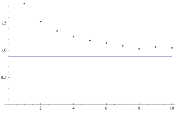
Figure 7: The coefficients $\beta_{N}$

The plot suggests that, if there is convergence at all, it will be to a higher value than $\beta$.

In order to understand what is going on, let us return to the coefficients $\bar{c}_{N}$ of table 1, and plot the combination

$$\tilde{c}_{N}:=\Gamma\left(1+\frac{N}{2}\right)\frac{\bar{c}_{N}}{\beta^{N}}\,.$$ (5.41)

If (5.37) were true, the coefficients would converge to the constant $c_{\infty}$; instead we find a curve which looks parabolic, see fig. 8.

Figure 8: The coefficients $\tilde{c}_{N}$

Therefore, let us look at yet another set of coefficients $c_{N}^{\prime}$,

$$c_{N}^{\prime}:=\frac{\tilde{c}_{N}}{N^{2}}\,.$$ (5.42)

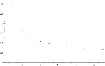
Figure 9: The coefficients $c_{N}^{\prime}$

These modified coefficients indeed seem to converge to a constant (see fig. 9); let us call this constant $c_{\infty}^{\prime}$. Thus we now have, instead of (5.37), the asymptotic behaviour

$$\bar{c}_{N}\stackrel{{\scriptstyle N\to\infty}}{{\sim}}\frac{c_{\infty}^{\prime}N^{2}\beta^{N}}{\Gamma(1+N/2)}\,.$$ (5.43)

Fortunately, this does not change anything essential: instead of (5.36) we get

$$\sum_{N=0}^{\infty}N^{2}\frac{x^{N}}{\Gamma(1+N/2)}\stackrel{{\scriptstyle x\to\infty}}{{\sim}}8x^{4}\,{\rm e}^{x^{2}}\,.$$ (5.44)

So, there is no modification of the exponent, only of the prefactor, which does not interest us right now. We can also adapt the definition (5.40) of $\beta_{N}$ to the asymptotic behavior (5.43) by defining

$$\beta_{N}^{\prime}:=\frac{N^{2}\bar{c}_{N+1}\Gamma\bigl{(}1+\frac{N+1}{2}\bigr{)}}{(N+1)^{2}\bar{c}_{N}\Gamma\bigl{(}1+\frac{N}{2}\bigr{)}}=\frac{\beta_{N}}{(1+1/N)^{2}}\,.$$ (5.45)

The first ten coefficients $\beta_{N}^{\prime}$ are given in table 3.

Table 3: The coefficients $\beta_{N}^{\prime}$.

$N$	1	2	3	4	5	6	7	8	9	10
$\beta_{N}^{\prime}$	$0.464$	$0.678$	$0.762$	$0.801$	$0.818$	$0.833$	$0.827$	$0.817$	$0.859$	$0.861$

From these values, it is at least credible that $\beta_{N}^{\prime}$ asymptotically converges to $\beta=0.886$; see fig. 10.

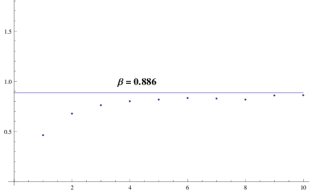
Figure 10: The coefficients $\beta_{N}^{\prime}$

In the following, we hence assume that (5.43) is true, with $\beta=\sqrt{\pi}/2$. Let us then undo the assumption of small $g$ and of the saddle point at $S=T=1$ and return to (LABEL:GNmaster2). The asymptotic summation formula (5.44) now leads to a total exponential factor

$${\rm exp}\biggl{[}-\hat{t}\Bigl{(}S+T+\frac{1}{S}+\frac{1}{T}-\pi^{2}g^{2}\frac{S^{2}T^{2}}{S+T}\Bigr{)}\biggr{]}\,.$$ (5.46)

As long as $g^{2}<1/3\pi^{2}$, one finds a saddle point (local maximum) of the exponent at

$$S=T=\sqrt{\frac{2}{3}}\frac{1}{\pi g}\sqrt{1-\sqrt{1-3\pi^{2}g^{2}}}$$ (5.47)

with saddle point value

$${\rm exp}\biggl{\{}-\hat{t}\frac{4\sqrt{2}}{3}\biggl{[}\bigg{(}1+\sqrt{1-3\pi^{2}g^{2}}\bigg{)}^{-1/2}+\bigg{(}1+\sqrt{1-3\pi^{2}g^{2}}\bigg{)}^{1/2}\biggr{]}\biggr{\}}\,.$$ (5.48)

From (5.3), (5.6) this gives for the lowest bound state mass $m_{0}$

$$\frac{m_{0}}{m} = \frac{2\sqrt{2}}{3}\biggl{[}\bigg{(}1+\sqrt{1-3\pi^{2}g^{2}}\bigg{)}^{-1/2}+\bigg{(}1+\sqrt{1-3\pi^{2}g^{2}}\bigg{)}^{1/2}\biggr{]}$$

As $g^{2}$ increases from zero to its maximal value $1/3\pi^{2}$, the result (LABEL:m0fin) for this mass $m_{0}$ decreases monotonically from $2m$ to $\frac{4\sqrt{2}}{3}m=1.886m$. An expansion of (LABEL:m0fin) in $g$ yields

$$\frac{m_{0}}{m} = 2-\frac{\pi^{2}g^{2}}{4}-\frac{9}{64}(\pi^{2}g^{2})^{2}-\frac{81}{512}(\pi^{2}g^{2})^{3}-\ldots$$ (5.50)

In the second term of the expansion we find again, of course, the nonrelativistic limit (5.32) of the binding energy, which we have already used as an input for our matching procedure; but the order $g^{4}$ term is already new. We note that in the expansion (5.50) of the bound state mass in powers of $g$ no term of the order $g^{3}\ln g$ appears, as it would be the case for the corresponding result in the Wick-Cutkosky model, i.e., for the ladder approximation of the Bethe-Salpeter equation in the same model theory [49]. As we have mentioned before in the introduction, such a contribution is generally considered to be unphysical.

Our result for the mass of the lowest bound state may be compared to the result of the relativistic eikonal approximation or Todorov’s equation [54, 55], in our notation,

$$\frac{m_{0}}{m} = \sqrt{2}\bigg{(}1+\sqrt{1-\pi^{2}g^{2}}\bigg{)}^{1/2}$$ (5.51)

$$= 2-\frac{\pi^{2}g^{2}}{4}-\frac{5}{64}(\pi^{2}g^{2})^{2}-\ldots$$

In terms of diagrams, the eikonal approximation sums up all ladder and crossed ladder diagrams, but neglects any self-energy contributions and vertex corrections, just as our approach does. It has been argued to reproduce the contribution of the ladder and crossed ladder diagrams correctly up to the order $g^{4}$ (see, e.g., [31]). Note that the coefficient of the $g^{4}$-term in the expansion (5.51) of the bound state mass in powers of the coupling constant is somewhat smaller (in absolute value) than in our approximation, but it has the same sign.

Finally, we can compare the maximal possible value of the coupling constant, $g^{2}=1/3\pi^{2}$, to the critical value found in the variational worldline approximation of [31]. The latter value is (approximately) $\alpha=0{.}814$ (without self-energy and vertex corrections, and for a massless exchanged particle), somewhat larger than our value $\alpha=\pi g=1/\sqrt{3}=0{.}577$. The existence of a critical coupling constant is attributed to the instability of the vacuum in the scalar model theory in [31].

6 Conclusions

To summarize, in this paper we have used the worldline formalism to derive integral representations for three classes of amplitudes - the $N$ - propagators, $N$ - half-ladders and the $N$ - ladders - in scalar field theory involving an exchange of $N$ momenta, and in each case have given a compact expression combining the $N!$ Feynman diagrams contributing to the amplitude. For the $N$ - propagators and $N$ - ladders we have given these representations in both $x$ and (off-shell) momentum space, for the $N$ - half-ladders in $x$ - space only. These amplitudes are not only of interest in their own right, but, being off-shell, can also been used as building blocks for many more complex amplitudes.

In particular, we have derived a compact expression for the sum of all ladder graphs with $N$ rungs, including all possible crossings of the rungs, which we use in section 5 to extract an approximate formula for the mass of the lowest-lying bound state, explicitly for the case of a massless particle exchange between the constituents. Technically, we apply a saddle point approximation to our formula for the $N$-rung ladders, after summing over all $N$. Before applying the saddle point approximation, however, we have made use of a Gaussian approximation in eq. (LABEL:GNmaster1) that leads to an important simplification in the formulas for the $N$-rung ladders. Both approximations exploit the large-time limit that is being considered for the extraction of the lowest-lying bound state, but it would certainly be more satisfying to have a way to arrive at an approximate formula for the lowest bound-state mass by taking advantage of the large-time limit in a single step, instead of using two consecutive approximations. Thus our procedure cannot claim mathematical rigor, but we think it is worth presenting it in any case. This is because, differently from previous attempts at this calculation [47, 48, 49, 50], in our approach the truncation to the non-crossed ladder graphs is induced naturally by the Gaussian approximation $\vec{v}=\vec{u}$, rather than done ad hoc from the beginning, and moreover our final result (LABEL:m0fin) for the mass of the lowest bound state does not display any obvious inconsistencies. Equation (LABEL:m0fin) is similar to the result of the relativistic eikonal approximation [54, 55], and the maximal value of the coupling constant for which a bound state is found in our approximation is comparable to the critical coupling constant in a variational worldline approximation [31]. We intend to further test our result by a direct numerical path integral calculation along the lines of [39], but taking advantage of the sophisticated worldline Monte Carlo technology developed in the meantime in [17, 15]. Our aim in the present paper has merely been to demonstrate the feasibility of extracting information on the bound states of a theory from an analytical evaluation of the worldline integrals, in an appropriate approximation.

Our second nontrivial application was to obtain a new two-parameter integral representation for a massless four-point $x$ - space integral of some importance in $N=4$ SYM theory [34, 35, 36, 37].

Coming to possible generalizations, it would be straightforward to extend our various master formulas to the case of scalar QED (i.e. scalar lines and photon exchanges). In the spinor QED case (fermion lines and photon exchanges) closed-form expressions for general $N$ could still be achieved using the worldline super-formalism [3], however at the cost of introducing additional multiple Grassmann integrals. For eventual extensions to the nonabelian case it may turn out essential to work with a path integral representation of the color degree of freedom, such as the one recently given in [56], rather than with explicit color factors. Finally, even a closed-form treatment of ladder graphs involving the exchange of gravitons between scalars or spinors - a completely hopeless task in the Feynman diagram approach due to the existence of vertices involving an arbitrary number of gravitons - may be feasible in the worldline formalism along the lines of [24, 25].

Acknowledgements: We would like to thank A. Davydychev, J. Henn and D.G.C. McKeon for discussions and correspondence. C.S. thanks D. Kreimer and the Mathematical Physics group of HUB for hospitality and discussions, as well as the HUB Gruppe Rechentechnik for access to their supercomputing facility. A.H., C.S. and R.T. thank CONACyT for financial support. A.W. acknowledges support by CIC-UMSNH and CONACyT project no. CB-2009/131787.

A Comparison with Feynman diagrams

Let us consider the term appearing in (LABEL:orderNpspace)

$$N!\int_{0}^{1}du_{1}\cdot\cdot\int_{0}^{1}du_{N}\,\bigg{[}p_{1}^{2}+m^{2}+\sum_{i}(k_{i}^{2}+2p_{1}\cdot k_{i})u_{i}+\sum_{i<j}2k_{i}\cdot k_{j}\big{(}u_{i}\theta(u_{j}-u_{i})+u_{j}\theta(u_{i}-u_{j})\big{)}\bigg{]}^{-N-1}$$ (A.1)

The integration region can be split into $N!$ subregions specified by a unique ordering $\sigma(i)$ of the indices $i=1,2,..,N$ so that $t_{i}=u_{\sigma(i)}$ are ordered as $1\geq t_{1}\geq t_{2}\geq...\geq t_{N}\geq 0$. Then each integration subregion contributes

$$N!\int_{0}^{1}dt_{1}\int_{0}^{t_{1}}dt_{2}\int_{0}^{t_{2}}dt_{3}\cdot\cdot\int_{0}^{t_{N-1}}dt_{N}\,\bigg{[}p_{1}^{2}+m^{2}+\sum_{i}(k_{\sigma(i)}^{2}+2k_{\sigma(i)}\cdot p_{1})t_{i}$$

$$\hskip 85.35826pt+\sum_{i<j}2k_{\sigma(i)}\cdot k_{\sigma(j)}\big{(}t_{i}\underbrace{\theta(t_{j}-t_{i})}_{=0}+t_{j}\underbrace{\theta(t_{i}-t_{j})}_{=1}\big{)}\bigg{]}^{-N-1}$$

$$=N!\int_{0}^{1}dt_{1}\int_{0}^{t_{1}}dt_{2}\int_{0}^{t_{2}}dt_{3}\cdot\cdot\int_{0}^{t_{N-1}}dt_{N}\,\bigg{[}p_{1}^{2}+m^{2}+\sum_{i}(k_{\sigma(i)}^{2}+2k_{\sigma(i)}\cdot p_{1})t_{i}+\sum_{i<j}2k_{\sigma(i)}\cdot k_{\sigma(j)}t_{j}\bigg{]}^{-N-1}$$

$$=N!\int_{0}^{1}dt_{1}\int_{0}^{t_{1}}dt_{2}\int_{0}^{t_{2}}dt_{3}\cdot\cdot\int_{0}^{t_{N-1}}dt_{N}\,\bigg{[}p_{1}^{2}+m^{2}+\sum_{i}\Big{[}(k_{\sigma(i)}^{2}+2k_{\sigma(i)}\cdot(p_{1}+\sum_{j=1}^{i-1}k_{\sigma(j)})\Big{]}t_{i}\bigg{]}^{-N-1}$$

$$={1\over p_{1}^{2}+m^{2}}\ {1\over(p_{1}+k_{\sigma(1)})^{2}+m^{2}}\ {1\over(p_{1}+k_{\sigma(1)}+k_{\sigma(2)})^{2}+m^{2}}\,\cdot\cdot\cdot\,{1\over(p_{1}+\sum_{i=1}^{N}k_{\sigma(i)})^{2}+m^{2}}$$ (A.2)

This shows that in each internal propagator flows the momentum as implied by momentum conservation at each vertex. The last integration above has been carried out by using the well-known formula

$${1\over A_{0}A_{1}A_{2}\cdot\cdot\cdot A_{N}}\!\! = \!\!N!\int_{0}^{1}dt_{1}\int_{0}^{t_{1}}dt_{2}\int_{0}^{t_{2}}dt_{3}\cdot\cdot\int_{0}^{t_{N-1}}dt_{N}\,$$

$$\times \!\!{1\over[A_{0}+(A_{1}-A_{0})t_{1}+(A_{2}-A_{1})t_{2}+\cdot\cdot\cdot+(A_{N}-A_{N-1})t_{N}]^{N+1}}$$

References

[1]
R.P. Feynman, Phys. Rev. 80, 440 (1950).
[2]
R.P. Feynman, Phys. Rev. 84, 108 (1951).
[3]
C. Schubert, Phys. Rep. 355, 73 (2001), hep-th/0101036.
[4]
Z. Bern and D. A. Kosower,
Phys. Rev. Lett. 66, 1669 (1991);
Nucl. Phys. B 379, 451 (1992)
[5]
M. J. Strassler,
Nucl. Phys. B 385, 145 (1992), hep-ph/9205205.
[6]
F. Bastianelli and P. van Nieuwenhuizen,
Nucl. Phys. B 389, 53 (1993), hep-th/9208059.
[7]
D.G.C. McKeon, Ann. Phys. (N.Y.) 224, 139 (1993).
[8]
M.G. Schmidt and C. Schubert,
Phys. Lett. B 318, 438 (1993), hep-th/9309055.