No Local Double Exponential Gradient Growth in Hyperbolic Flow for the 2d Euler equation

Abstract.

We consider smooth, double-odd solutions of the two-dimensional Euler equation in $[-1,1)^{2}$ with periodic boundary conditions. This situation is a possible candidate to exhibit strong gradient growth near the origin. We analyze the flow in a small box around the origin in a strongly hyperbolic regime and prove that the compression of the fluid induced by the hyperbolic flow alone is not sufficient to create double-exponential growth of the gradient.

1. Introduction

The question whether solutions of the two-dimensional Euler equation in vorticity form

(1) $$\omega_{t}+u\cdot\nabla\omega =0,\quad u=\nabla^{\perp}(-\Delta)^{-1}\omega$$

($\nabla^{\bot}=(-\partial_{x_{2}},\partial_{x_{1}})$) can exhibit strong gradient growth in time is a topic of ongoing interest. The best known upper bound predicts double-exponential growth in time:

(2) $$\|\nabla\omega(\cdot,t)\|_{L^{\infty}(\Omega)}\leq C_{1}\exp(C_{2}\exp(C_{3}t))$$

on a domain $\Omega$ with either a smooth boundary with no-flow boundary condition or no boundary (e.g. a torus). The constants $C_{i}$ depend on the initial data. A natural and important question is: Are there flows for which this upper bound is attained? For domains with boundary, a recent breakthrough by A. Kiselev and V. Šverák [8] answers the question affirmatively. In [8], solutions are constructed that attain the double-exponential bound (2).

For smooth solutions on the torus, the situation is far from clear. The best known result so far was given by S. Denisov. In [4], he shows that at least superlinear gradient growth is possible and in [5] he provides an example of double-exponential growth for an arbitrarily long, but finite time interval. In the recent paper [11], A. Zlatoš constructs initial data leading to exponential gradient growth, his solution is however in $C^{1,\gamma}$ for some $\gamma\in(0,1)$ and not in $C^{2}$.

In [8] the construction is based on creating a hyperbolic flow scenario. By imposing a symmetry on the solutions, a stagnant point of the flow is created on the boundary of the domain. The initial conditions are chosen in such a way the flow on the boundary is directed towards the stagnant point, creating a strong fluid compression and therefore strong gradient growth.

A natural way to carry the Kiselev-Šverák construction to the torus is to consider double-odd solutions, i.e.

(3) $$\omega(-x_{1},x_{2}) =-\omega(x_{1},x_{2}),~{}\omega(x_{1},-x_{2})=-\omega(x_{1},x_{2}),$$

This construction was employed in [11]. In [5], a perturbation argument starting from a non-smooth double-odd stationary solution (see [1]) was used. So far, however, creating infinite-time double-exponential growth in the double-odd scenario was not succesful. Our goal in this paper is to explore the difficulties in using this scenario, by proving a conditional regularity result.

It is interesting to notice that the result [8] is in some sense analogous to the still open blowup problem for for the more singular surface quasigeostrophic equation. In SQG blowup means that the solution becomes singular in finite time whereas for the 2d Euler equation “blowup” would mean maximal (double-exponential) gradient growth on an infinite time interval. There are important conditional regularity results for the SQG equation such as [2, 3], where the authors study a certain blowup scenario, in order to finally exclude it. An analogous “conditional regularity result” for 2d Euler equation would be to show that in certain scenarios maximal gradient growth does not occur. Since the possible motions of fluids are various and in general very complicated, studying scenarios is an invaluable method to gain insight into regularity problems of fluid mechanics.

Our main result states that a hyperbolic flow cannot create double-exponential gradient growth near the origin by itself when we start with double-odd $C^{2}$ initial data, provided a certain “upstream” control is assumed on the flow. This is an important step into understanding the double-odd hyperbolic scenario since we rule out the most promising candidate for a mechanism creating maximal gradient growth, i.e. the local hyperbolic compression. Our result does not imply impossibility of double-exponential growth in general, but makes the construction of examples much harder.

In some sense, the scenario considered here is complementary to the one considered by D. Cordoba for the SQG equation in [2], where a closing hyperbolic saddle is considered. There the solution stays smooth except for the possible closing of the saddle. In our scenario for 2d Euler, the hyperbolic saddle is fixed due to the symmetry ($\omega=0$ on the coordinate axes), and we are asking if blowup can happen in another way.

We strongly believe that the techniqes developed here will also be useful in understanding the hyperbolic scenario for other models in fluid mechanics and also in situations with a physical boundary. There, although the goal is to prove the existence of a blowup, a certain amount of control up to the blowup time is necessary.

Interesting results concerning the related question of existence of double-exponential growth in the context of (nonsmooth) patch solutions were given by S. Denisov (see [6]).

Finally, we would like to mention the recent preprint [7], where a different approach is proposed to study whether double-exponential gradient growth can occur at an interior point.

1.1. Setup and feeding conditions.

We consider (1) on $\mathbb{T}=[-1,1)^{2}$ with periodic boundary conditions and double-odd $C^{2}$ initial data $\omega_{0}$. From now on, we use $\|\cdot\|_{\infty}$ to denote the $L^{\infty}$-norm on the torus $\mathbb{T}$.

The double-odd symmetry is preserved by the evolution and (3) implies that the origin is a stagnant point of the flow field for all times. Moreover, the flow on each coordinate axis is always directed along that axis. When considering smooth solutions $\omega\in C^{1}([0,\infty),C^{2}(\mathbb{T}))$, (3) also implies

$$\omega=0$$

on the coordinate axes.

We will study the flow in boxes of the form

$$D =(0,\delta_{1})\times(0,\delta_{2}),~{}~{}\widehat{D}=(0,\delta_{1}+\delta_{3})\times(0,\delta_{2}),$$

where $\delta_{j}$ are positive, but small and

$$0<\delta_{1}<\delta_{2}<\delta_{1}+\delta_{3}.$$

In a hyperbolic flow, the origin is a stagnant point of the flow and fluid particles constantly enter the box $D$ from the right and leave on the top (see Fig. 1). The particles moving on the $x_{1}$-axis approach asymptotically the origin and never leave the box $D$. Generally speaking, there is, a compression of the fluid in $x_{1}$-direction and a decompression in $x_{2}$-direction (or the other way around). The vorticity is zero on the axes. The gradient growth in the box $D$ comes from two sources: particles that were at $t=0$ inside $D$ and those which enter the box at later times. The time evolution of the gradient of those particles entering the box is difficult to control over infnite times, and is generated by flow situations which have little to do with the hyperbolic scenario. We are interested in making local statements and must assume a certain control on the flow entering the box $D$.

We shall therefore call $\widehat{D}\setminus D$ feeding zone and formalize this idea in the following definition (the meaning of the parameter $\alpha$ will become clear later).

Definition 1.1.

Let $\alpha\in(0,\frac{1}{4})$. The box $\widehat{D}$ is said to satisfy the conditions of controlled feeding, with feeding parameter $R\geq 0$ if

(4) $$\left|\frac{\partial\omega}{\partial x_{1}}(x,t)\right|\leq Rx_{2}^{1-\alpha},~{}~{}\left|\frac{\partial\omega}{\partial x_{2}}(x,t)\right|\leq R\quad(x\in\widehat{D}\setminus D)$$

for all times $t\geq 0$.

We can think of the first inequality in (4) as a Hölder-version of a bound on $\partial_{x_{2},x_{1}}\omega$, keeping in mind that $\partial_{x_{1}}\omega(x_{1},0,t)=0$ for all times. The concept of controlled feeding conditions allows us to study the evolution of $\omega$ in $D$ independent of the remaining flow. Note that for the purposes of this paper, we consider time-independent $R$ only (see also Remark 2.1).

1.2. The hyperbolic scenario.

In order to give a definition of hyperbolic flow suitable for our purposes, we introduce the following important quantity. Let $\alpha\in(0,\frac{1}{4})$ be fixed. For a smooth, periodic function $\omega$ we set

$$M(x,t):=\max_{0\leq y_{1},y_{2}\leq\max\{x_{1},x_{2}\}}\left\{\left|y_{1}^{\alpha}\frac{\partial\omega}{\partial x_{1}}(y,t)\right|,\left|y_{2}^{\alpha}\frac{\partial\omega}{\partial x_{2}}(y,t)\right|\right\}+\|\omega\|_{\infty}.$$

Note that $M(x,t)$ also depends on $\omega$ and $\alpha$. The velocity field $u(x,t):=\nabla^{\bot}(-\Delta)^{-1}\omega$ for double-odd $\omega$ ($\omega$ with mean zero over $\mathbb{T}$) can be written in the form

(5) $$u_{1}(x,t)=-x_{1}Q_{1}(x,t),~{}u_{2}(x,t)=x_{2}Q_{2}(x,t)$$

where $Q_{1},Q_{2}$ are scalar fields given by certain integral operators (see (14)) acting on $\omega$. The following definition states that we regard the flow as hyperbolic if both $Q_{1}$ and $Q_{2}$ essentially have a positive lower bound, up to a term controlled by the quantity $M(x,t)$.

Definition 1.2.

Let $\omega$ be a smooth solution of the Euler equation, and let $\alpha\in(0,\frac{1}{4})$ be fixed. We say that the flow is hyperbolic near the origin if there are constants $\rho,A,\beta_{0}>0$ for which the following condition is satisfied for all $t\in[0,\infty)$:

(6) $$Q_{i}(x,t)+A|x|^{1-\alpha}M(x,t)\geq\beta_{0}>0\qquad(0\leq x_{1},x_{2}\leq\rho,~{}i=1,2).$$

The model situation for a hyperbolic flow is the following: Consider the dynamical system

$$\dot{x}_{1} =-Ax_{1},~{}~{}\dot{x}_{2}=Bx_{2}$$

with positive constants $A,B$. This system has a hyperbolic saddle point in $(0,0)$, which is a stagnant point of the flow. On the axes, the flow is directed along the axes.

The velocity field given by (5) generalizes this structure if $Q_{i}(x,t)\geq\beta_{0}>0$. A further generalization necessary for our result is (6), since the stronger condition $Q_{i}(x,t)\geq\beta_{0}>0$ cannot be easily realized. In certain flow situations, the term $|x|^{1-\alpha}M(x,t)$ is small close to the origin. Bounding the quantity $M(x,t)$ plays a central role in our estimates.

Remark 1.3.

By choosing the initial data $\omega_{0}$ suitably, we can ensure hyperbolic flow. One possible choice is, for example, choosing $\omega_{0}$ to be nonnegative in $[0,1]^{2}$ and such that $\omega_{0}=1$ on a set of sufficiently large measure, as it was done in [8, 11]. This creates a situation where (6) is satisfied (see theorem 4.2). In this sense, (6) is a “realistic” condition on the flow.

1.3. Main result.

Our main result is the following theorem.

Theorem 1.4.

Fix $0<\alpha<\frac{1}{4},0<\delta_{3}<1/2$. Let $\omega$ be a $C^{2}$, double-odd solution of the Euler equation with initial data $\omega_{0}$, and suppose the flow is hyperbolic near the origin. Let $R>\|\omega_{0}\|_{\infty}>0$ be given. Then there exist small $\delta_{1},\delta_{2}>0$ depending on $\alpha,\beta_{0},R$ and $\omega_{0}$, such that if $\widehat{D}$ satisfies the controlled feeding conditions with parameter $R$, then

$$\|\nabla\omega\|_{D,\infty}\leq C_{1}\exp(C_{2}t)\quad(t\in[0,\infty))$$

for some $C_{1},C_{2}>0$ depending on $R,\alpha,\beta_{0},\delta_{1},\delta_{2},\delta_{3},\omega_{0}$.

This means that the hyperbolic compression alone and the interaction of the fluid inside the box is not sufficient to create double-exponential gradient growth. One would have to create a scenario where the feeding conditions are violated. This means roughly that there has to be a kind of compression in $x_{2}$-direction in the feeding zone. This would have to be caused by much more complicated interactions outside the box. At the present time, no such scenario is known.

2. Gradient growth in the hyperbolic scenario

Before describing our approach, let us explain first why at first sight the hyperbolic scenario seems to be a good candidate for double-exponential growth. Namely, for $Q_{1},Q_{2}$ we have the upper bounds

$$Q_{1}(x,t),Q_{2}(x,t)\lesssim\|\omega\|_{\infty}|\log(x_{1}^{2}+x_{2}^{2})|.$$

If it were possible to create a situation where a lower bound of roughly the same order holds, i.e. $Q_{1}\geq C|\log(x_{1}^{2}+x_{2}^{2})|$ over an infinitely long time interval, then for the particle trajectories lying on the $x_{1}$-axis (i.e. $X_{2}=0$)

$$X_{1}(t)\leq\exp(-C_{1}\exp(C_{2}t))$$

would hold, as seen by solving the ODE $\dot{X}_{1}=-X_{1}Q_{1}$. If, moreover, one could arrange for the initial data $\omega_{0}$ to have suitable nontrivial values on the $x_{1}$-axis, then this would create double exponential gradient growth. However, the simultaneous requirements of smoothness and double-odd symmetry of $\omega$, necessarily imply $\omega=0$ on the axes. Moreover, it is highly unclear how a such strong lower bound on $Q_{1}$ could be achieved. As we shall see later, a certain amount of smoothness of $\omega$ and the vanishing of $\omega$ on the axes lead to a better upper bound, without the logarithmic behavior which is crucial for the double-exponential growth.

Another way one might hope to get double exponential growth is to consider a “projectile”, i.e. to track the movement of a small domain close to the origin on which $\omega=1$, as it was done in [8]. There the self-interaction of the projectile was able to create enough growth in the values of $Q_{1}$ to allow double-exponential growth. While the projectile approaches the origin, the values of $Q_{1}$ on it get larger, this fact being connected to a certain logarithmically divergent integral. Our Theorem 1.4 shows that in general this is not possible for double-odd solutions, unless there is some kind of compression in $x_{2}$-direction in the feeding zone. Thus a scenario with maximal gradient growth must be much more complicated than using the self-interaction of the projectile.

In fact, provided the feeding condition holds, the steady fluid compression guaranteed by (6) will turn out to stabilize the flow in the neighborhood of the origin. That is, the hyperbolicity condition (6) - which is essentially a lower bound on $Q_{i}$ - is converted in the proof of Theorem 1.4 into an upper bound for $Q_{i}$. This is what finally leads to a bound on the gradient growth in $D$.

2.1. Heuristic considerations.

We now present an intuitive discussion of our result. Fluid particles carried by the hyperbolic flow will constantly enter the box $D$ from the right and leave on the top (see figure 1). All particles except for those moving on the axes spend a finite time in the box. The particles on the $x_{1}$-axis move towards the left approaching the origin asymptotically as $t\to\infty$. Particle trajectories $t\mapsto\mathbf{X}(t)=(X_{1}(t),X_{2}(t))$ for which $X_{2}(0)$ is small approximate the straight trajectories of the particles on the $x_{1}$-axis for a long time, before going steeply upward. The time a particle spends in $D$ goes to infinity as $X_{2}(0)\to 0$.

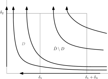
Figure 1. Illustration of a hyperbolic flow.

We now consider the trajectory of a particle $\mathbf{X}$. The particle may have started inside $D$ at time $t=0$, or may have entered the box at some time $T_{0}>0$, in which case $\mathbf{X}(T_{0})\in\partial D$. Also, assume that the particle exits the box $D$ at some time $T_{e}$, i.e. $X_{2}(T_{e})=\delta_{2}$. The evolution of the gradient of $\omega$ along the trajectory is given by an ODE of the form

(7) $$\frac{d}{dt}\nabla\omega(\mathbf{X}(t),t)=(-\nabla u(\mathbf{X}(t),t))^{T}\nabla\omega(\mathbf{X}(t),t)$$

where $\nabla u$ is the velocity gradient. The relation (7) is simply derived by differentiating the Euler equation. The key is now to use the structure (5) of the velocity field such that we obtain

(8) $$\frac{d}{dt}\nabla\omega(\mathbf{X}(t),t)=\begin{pmatrix}Q_{1}+x_{1}\frac{\partial Q_{1}}{\partial x_{1}}&-x_{2}\frac{\partial Q_{2}}{\partial x_{1}}\\ x_{1}\frac{\partial Q_{1}}{\partial x_{2}}&-Q_{2}-x_{2}\frac{\partial Q_{2}}{\partial x_{2}}\end{pmatrix}\nabla\omega(\mathbf{X}(t),t)$$

We write the right hand side of (8) as

$$\begin{pmatrix}a(t)&c(t)\\ b(t)&-a(t)\end{pmatrix}\nabla\omega(\mathbf{X}(t),t).$$

evaluating all matrix entries along the given trajectory $\mathbf{X}$. Note that the matrix has trace zero, since the velocity field $u$ is divergence free. There are several ways we can heuristically regard (8) as a perturbation of an easier problem.

• For the discussion assume that $Q_{1},Q_{2}>0$ and we can control the derivatives $\partial_{x_{j}}Q_{i}$ for small $x$. Since in a sufficiently small box $x_{1}\partial_{x_{1}}Q_{1},x_{2}\partial_{x_{2}}Q_{2}$ should be rather “small” (due to the prefactors $x_{1},x_{2}$), $a$ should be positive and bounded away from zero along the hyperbolic trajectory. To gain some insight, we consider the case of a particle moving close to the $x_{1}$-axis, i.e. with small $X_{2}(T_{0})>0$. We expect that $c=-x_{2}\partial_{x_{1}}Q_{2},b=x_{1}\partial_{x_{2}}Q_{1}$ are “small”. Life would be easy if we could neglect $b,c$ and set $b,c=0$ in (8), so that we have a diagonal system. Denoting $\boldsymbol{\xi}(t)=\nabla\omega(\mathbf{X}(t),t)$ the solution can be explicitly computed to be

  (9) $$\xi_{1}(t)=e^{A(t)}\xi_{1}(T_{0}),~{}~{}\xi_{2}(t)=e^{-A(t)}\xi_{2}(T_{0}).$$

  where $A(t)=\int_{T_{0}}^{t}a(\mathbf{X}(s))~{}ds$. (9) shows that, in general, the gradient in $x_{1}$-direction grows along the particle trajectory. However, there is an effect which allows us to cancel the growing factor $e^{A}$. Assume for the sake of the discussion that the following stronger feeding conditions hold:

  (10) $$\left|\frac{\partial\omega}{\partial x_{1}}(x,t)\right|\leq Rx_{2},~{}~{}\left|\frac{\partial\omega}{\partial x_{2}}(x,t)\right|\leq R,$$

  on $\widehat{D}$ for $t=0$ and on $\widehat{D}\setminus D$ for all $t>0$. These imply in either case $T_{0}=0$ and $T_{0}>0$

  (11) $$|\xi_{1}(t)|\leq e^{A(t)}|\xi_{1}(T_{0})|=e^{A(t)}\left|\frac{\partial\omega}{\partial x_{1}}(\mathbf{X}(T_{0}),T_{0})\right|\leq Re^{A(t)}X_{2}(T_{0}).$$

  Now we observe that

  (12) $$A(t)\approx\int_{T_{0}}^{t}Q_{2}(s)~{}ds$$

  temporarily neglecting the “small” term $x_{2}\partial_{x_{2}}Q_{2}$. Now from (5) we have the differential equation $\dot{X}_{2}=X_{2}Q_{2}$, so that $X_{2}(t)=X_{2}(T_{0})\exp\left(\int_{T_{0}}^{t}Q_{2}(\mathbf{X}(s))~{}ds\right)$ and hence

  (13) $$X_{2}(T_{0})=X_{2}(T_{e})\exp\left(-\int_{T_{0}}^{T_{e}}Q_{2}(\mathbf{X}(s))~{}ds\right)\leq\delta_{2}\exp\left(-\int_{T_{0}}^{T_{e}}Q_{2}(\mathbf{X}(s))~{}ds\right).$$

  Combining (13), (11) and (12), we get

  $$|\xi_{1}(t)|\leq\delta_{2}R\exp\left(-\int_{t}^{T_{e}}Q_{2}(\mathbf{X}(s))~{}ds\right)\leq\delta_{2}R,$$

  suggesting that the gradient in $x_{1}$-direction does not grow at all in time given the feeding condition (10). Our rigorous result does not give such a strong conclusion, but we will be able to prove that the gradient grows at most exponentially in time using a weaker feeding condition. In Remark 4.6 we explain why (10) is not an appropriate feeding condition for the problem.

The heuristics appear deceivingly simple, but in order to make the argument rigorous, we have to overcome a number of formidable technical difficulties. To begin with, the coefficients of (8) depend on the solution $\omega$ through the integral operators $Q_{1},Q_{2}$. The derivatives $\partial_{x_{1}}Q_{1},\partial_{x_{2}}Q_{2}$ are given by singular integral operators.

Of course, none of the coefficients may be neglected, and we have to produce sufficiently good estimates on the solutions of the full ODE system (8). A major obstacle in getting good estimates, however, is caused by the unstable nature of (8). To illustrate this we consider a tridiagonal system by setting $c=0$, but keeping $b$, so that we get a supposedly better approximation than the diagonal system. In this model, too, the solutions can be calculated explictly, and we get

$$\xi_{1}(t)=e^{A(t)}\xi_{1}(T_{0}),~{}~{}\xi_{2}(t)=e^{-A(t)}\left[\xi_{2}(T_{0})+\xi_{1}(T_{0})\int_{0}^{t}b(s)e^{2A(s)}~{}ds\right].$$

This shows that not only the derivative in $x_{1}$-direction but also the derivative in $x_{2}$-direction of $\omega$ may potentially grow in time (due to the contribution $e^{-A(t)}\int_{0}^{t}b(s)e^{2A(s)}~{}ds$). To make things worse, a possible strong growth in $\partial_{x_{2}}\omega$ is coupled back into the coefficients of the ODE (8) via our estimates on $\partial_{x_{1}}Q_{1},\partial_{x_{2}}Q_{2}$. On the other hand, by a similar argumentation as in the case of the diagonal system, the factor $\xi_{1}(T_{0})$ may help via a feeding condition. We need therefore to proceed with extreme care, looking to cancel the growing factor $e^{A}$ with the decaying factor $e^{-A}$ whenever possible.

Remark 2.1.

In our scenario, we always assume the intensity of the feeding (i.e. the quantity $R$) to be time-independent. One might think of allowing the feeding parameter to grow in time to include more complicated scenarios. However, this is met with considerable challenges.

Firstly, it is not clear what a realistic condition on $R$ should be, since it depends on the complexity of the flow away from the origin. One concrete situation where we can imagine a reasonable time-dependent feeding condition is as follows: A vortex created by a large patch (see Figure 2) where $\omega$ is constantly $1$. The flow revolves in clock-wise direction around the patch and, in analogy with a shear flow, one could assume linear growth in time of the gradient in the feeding zone.

The application of the techniques developed here to time-dependent feeding are not straightforward (see Remark 7.3), due to the non-local and non-linear nature of the problem.

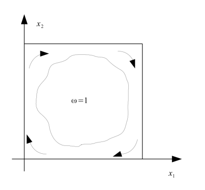
Figure 2. Flow around a patch.

3. Notation

3.1. Euler velocity field.

For $x=(x_{1},x_{2})$ we write $\widetilde{x}=(-x_{1},x_{2})$ and $\overline{x}=(x_{1},-x_{2})$. The velocity field for the Euler equation is

$$u(x,t)=\frac{1}{2\pi}\int_{\mathbb{R}^{2}}\frac{(y-x)^{\bot}}{|y-x|^{2}}\omega(y,t)~{}dy$$

where $\omega\in C^{2}(\mathbb{T})$ is periodically extended to all of $\mathbb{R}^{2}$ and $z^{\bot}=(-z_{2},z_{1})$. In the calculation of the integral a limit in the mean (sequence of unboundedly growing domains) is understood. Note that the velocity field is $\nabla^{\bot}(-\Delta)^{-1}\omega$, where $-\Delta$ is the periodic Laplacian on the Torus $\mathbb{T}$. A simple calculation using the double-odd symmetry of $\omega$ leads to

$$u_{1}(x,t)=-x_{1}Q_{1}(x,t),~{}~{}u_{2}(x,t)=x_{2}Q_{2}(x,t)$$

where $Q_{1},Q_{2}$ are the following integral operators (see Appendix B)

(14) $$\begin{split}Q_{1}(x,t)&=c_{0}\int_{[0,1]^{2}}[G_{1}^{1}(x,y)+G_{1}^{2}(x,y)]\omega(y,t)~{}dy+Q_{1}^{r}(x,t)\\ Q_{2}(x,t)&=c_{0}\int_{[0,1]^{2}}[G_{2}^{1}(x,y)+G_{2}^{2}(x,y)]\omega(y,t)~{}dy+Q_{2}^{r}(x,t)\end{split}$$

with kernels

$$G_{1}^{1}(x,y)=\frac{y_{1}(y_{2}-x_{2})}{|y-x|^{2}|y-\widetilde{x}|^{2}}, G_{1}^{2}(x,y)=\frac{y_{1}(y_{2}+x_{2})}{|y+x|^{2}|y-\overline{x}|^{2}},$$

$$G_{2}^{1}(x,y)=\frac{y_{2}(y_{1}+x_{1})}{|y+x|^{2}|y-\widetilde{x}|^{2}}, G_{2}^{2}(x,y)=\frac{y_{2}(y_{1}-x_{1})}{|y-x|^{2}|y-\overline{x}|^{2}},$$

where $c_{0}$ denotes the right constant. The expression $Q_{1}^{r}$ is given by the following (limit in the mean) integral

$$c_{0}\int_{\mathbb{R}^{2}_{+}\setminus{[0,1]^{2}}}[G_{1}^{1}(x,y)+G_{1}^{2}(x,y)]\omega(y)~{}dy,\qquad\mathbb{R}^{2}_{+}=(0,\infty)^{2},$$

a similar formula holding for $Q_{2}^{r}$.

In section 4 we will derive estimates for the entries of the matrix in (8) which are independent of the trajectory. For this purpose it is convenient to use the definitions:

(15) $$\begin{split}&a(x,t):=Q_{1}(x,t)+x_{1}\frac{\partial Q_{1}}{\partial x_{1}}(x,t)=Q_{2}(x,t)+x_{2}\frac{\partial Q_{2}}{\partial x_{2}}(x,t),\\ &b(x,t):=x_{1}\frac{\partial Q_{1}}{\partial x_{2}}(x,t),\\ &c(x,t):=-x_{2}\frac{\partial Q_{2}}{\partial x_{1}}(x,t).\end{split}$$

Moreover, since the estimates will be for fixed $t$ we shall often skip the $t$ variable in the notation. When evaluating $a,b,c,Q_{i}$ etc. along a particle trajectory $\mathbf{X}(t)$ in section 6 we shall write $a(t):=a(\mathbf{X}(t),t)$ etc. reconciling with the notation in section 2.1.

3.2. Convention for estimates.

The notation $f\lesssim g$ means

$$f\leq Cg,$$

where $C$ may depend on $\alpha,\beta,\|\omega\|_{\infty}$ and on universal constants, e.g. geometrical characteristics of the domain $\mathbb{T}$. $C$ does not depend on $\delta_{1},\delta_{2},\delta_{3},t$. When using this notation, we shall always imply that $C<\infty$ for all $\alpha\in(0,\frac{1}{4})$.

4. Potential theory of $Q_{1},Q_{2}$

4.1. Sufficient conditions for hyperbolic flow

We will be working with boxes of the form

$$D =(0,\delta_{1})\times(0,\delta_{2})$$

(16) $$\widehat{D} =(0,\delta_{1}+\delta_{3})\times(0,\delta_{2}),$$

with the following restriction:

(17) $$0<\delta_{1}<\delta_{2}<\delta_{1}+\delta_{3}.$$

and $\delta_{j}$ so small that $\widehat{D}\subset[0,1]^{2}$. We also write

$$d(x)=\delta_{2}-x_{2}$$

which is the distance of the point $x$ to the top of the box. We write $\boldsymbol{\delta}=(\delta_{1},\delta_{2}),|\boldsymbol{\delta}|^{2}=\delta_{1}^{2}+\delta_{2}^{2}$.

Define

$$M_{D}(t):=\max_{y\in D}\left\{\left|y_{1}^{\alpha}\frac{\partial\omega}{\partial x_{1}}(y,t)\right|,\left|y_{2}^{\alpha}\frac{\partial\omega}{\partial x_{2}}(y,t)\right|\right\}+\|\omega\|_{\infty}$$

and $M_{\widehat{D}}$ for the analogous quantity. Note that $M_{D}$ and $M_{\widehat{D}}$ depend on $\omega$ and $\alpha$.

As mentioned before, the flow near the origin can be made hyperbolic, with compression in the $x_{1}$-direction and expansion in $x_{2}$-direction by choosing the initial data such that $\omega_{0}\geq 0$ on ${[0,1]^{2}}$ and such that

$$\mathfrak{m}:=|\{x:\omega_{0}(x)=\|\omega_{0}\|_{\infty}\}|$$

is sufficiently large. This is a consequence of theorem 4.2.

Remark 4.1.

1. As a consequence of $\omega=0$ on the coordinate axes we have the following important inequality

   (18) $$|\omega(y,t)|\lesssim M(x,t)\,y_{j}^{1-\alpha}\qquad(y_{1},y_{2}\leq\max\{x_{1},x_{2}\})$$

   where $j=1,2$.

2. The periodicity and double-oddness of $\omega(\cdot,t)$ imply also the reflection symmetries

   $$\omega(1+x_{1},x_{2},t)=-\omega(1-x_{1},x_{2},t),~{}\omega(x_{1},1+x_{2})=-\omega(x_{1},1-x_{2}).$$

   Consequently, the four corner points of $[-1,1]\times[-1,1]$ are also stagnant points of the flow, the flow being confined in ${[0,1]^{2}}$. Hence $\omega_{0}\geq 0$ on ${[0,1]^{2}}$ implies $\omega(x,t)\geq 0$ on ${[0,1]^{2}}$ for all times, a fact we shall use below.

Theorem 4.2.

Suppose $\omega_{0}(x)\geq 0$ on ${[0,1]^{2}}$. There exist universal $0<m_{0}<1$ and $0<K$ such that if $m_{0}<\mathfrak{m}<1$, there are $\beta_{0}>0,A>0$ such that the following estimates hold for all times

(19) $$\begin{split}Q_{2}(x,t)+AM(x,t)|x|^{1-\alpha}\geq\beta_{0}\\ Q_{1}(x,t)+AM(x,t)|x|^{1-\alpha}\geq\beta_{0}\end{split}$$

for $|x|\leq K(1-\mathfrak{m})$, i.e. the flow is hyperbolic near the origin.

To prove this, we need the following Lemma, which is an adaption of a result in [11].

Lemma 4.3.

Let $\Omega(2x):=[2x_{1},1]\times[2x_{2},1]$. Suppose $\omega(x)\geq 0$ for $x\in{[0,1]^{2}}$. Then the estimate

$$Q_{i}(x,t)\geq c_{0}\int_{\Omega(2x)}\frac{y_{1}y_{2}}{|y|^{4}}\omega(y,t)~{}dy-C_{1}M(x,t)|x|^{1-\alpha}-C_{2}\|\omega\|_{\infty}\quad(x\in D,~{}i=1,2)$$

holds, with universal $C_{1},C_{2}>0$.

Proof.

We prove the result for $Q_{2}$, the proof for $Q_{1}$ is similar. We have

$$Q_{2}(x)\geq c_{0}\int_{\Omega(2x)}\frac{y_{1}y_{2}}{|y|^{4}}\omega(y)~{}dy+c_{0}\int_{\Omega(2x)}\left[G_{2}^{2}(x,y)-\frac{y_{1}y_{2}}{|y|^{4}}\right]\omega(y)~{}dy$$

$$+c_{0}\int_{{[0,1]^{2}}\setminus\Omega(2x)}G_{2}^{2}(x,y)\omega(y)~{}dy-C_{1}\|\omega\|_{\infty},$$

throwing away the nonnegative contribution from $G_{2}^{1}$ and estimating $Q_{2}^{r}$ by $C_{1}\|\omega\|_{\infty}$ for $x\in D$. First, note that straightforward calculations and estimations give

$$\left|G_{2}^{2}(x,y)-\frac{y_{1}y_{2}}{|y|^{4}}\right|=\frac{|y|^{4}y_{2}(y_{1}-x_{1})-|y-x|^{2}|y-\overline{x}|^{2}y_{1}y_{2}}{|y|^{4}|y-x|^{2}|y-\overline{x}|^{2}}.$$

Using

$$|y-x|^{2} =|y|^{2}-2x\cdot y+|x|^{2}$$

$$|y-\overline{x}|^{2} =|y|^{2}-2\overline{x}\cdot y+|x|^{2}$$

the nominator can be estimated by

$$\sum_{j=1}^{4}|x|^{j}|y|^{6-j}.$$

For the denominator, note that $y\in\Omega(2x)$ implies that $|y-x|\geq\frac{1}{2}|y|,|y-\overline{x}|\geq\frac{1}{2}|y|$, i.e. the denominator is $\gtrsim|y|^{8}$. Hence, the integral over $\Omega(2x)$ is bounded in absolute value by

$$\|\omega\|_{\infty}\sum_{j=1}^{4}|x|^{j}\int_{2\geq|y|\geq 2|x|}|y|^{-2-j}dy\lesssim 1.$$

For the estimation of the integral with domain of integration ${[0,1]^{2}}\setminus\Omega(2x)$, we distinguish two cases. The more difficult case is given by the condition $x_{2}\leq x_{1}$, and we split the domain of integration into the three parts $[2x_{1},1]\times[0,2x_{2}],[0,2x_{1}]\times[2x_{1},1]$ and $[0,2x_{1}]\times[0,2x_{1}]$. For the integral over $[2x_{1},1]\times[0,2x_{2}]$, estimate $\omega$ by its $L^{\infty}$-norm and in the remaining integral we substitute $y_{j}=x_{j}+z_{j}$.

$$\int_{x_{1}}^{1-x_{1}}\int_{-x_{2}}^{x_{2}}\frac{z_{1}(x_{2}+z_{2})}{(z_{1}^{2}+z_{2}^{2})(z_{1}^{2}+(2x_{2}+z_{2})^{2})}~{}dz\leq\int_{0}^{1}\int_{-x_{2}}^{x_{2}}\frac{2z_{1}x_{2}}{(z_{1}^{2}+z_{2}^{2})(z_{1}^{2}+x_{2}^{2})}~{}dz_{2}~{}dz_{1}$$

$$\lesssim\int_{0}^{1}\frac{z_{1}x_{2}}{(z_{1}^{2}+x_{2}^{2})}\frac{1}{z_{1}}\arctan(x_{2}/z_{1})~{}dz_{1}\lesssim\arctan(1/x_{2})\lesssim 1.$$

The same strategy for the integral over $[0,2x_{1}]\times[2x_{1},1]$ leads to

$$\int\limits_{-x_{1}}^{x_{1}}\int\limits_{2x_{1}-x_{2}}^{1-x_{2}}\frac{|z_{1}|(x_{2}+z_{2})}{(z_{1}^{2}+z_{2}^{2})(z_{1}^{2}+(2x_{2}+z_{2})^{2})}~{}dz \leq 2\int\limits_{0}^{x_{1}}\int\limits_{x_{1}}^{1}\frac{z_{1}(x_{2}+z_{2})}{(z_{1}^{2}+z_{2}^{2})(z_{1}^{2}+(2x_{2}+z_{2})^{2})}~{}dz.$$

Noting

$$\int\limits_{0}^{x_{1}}\int\limits_{x_{1}}^{1}\frac{z_{1}x_{2}}{(z_{1}^{2}+z_{2}^{2})(z_{1}^{2}+(2x_{2}+z_{2})^{2})}~{}dz\leq\int\limits_{0}^{x_{1}}\int\limits_{x_{1}}^{1}\frac{z_{1}x_{2}}{(z_{1}^{2}+z_{2}^{2})(z_{1}^{2}+x_{2}^{2})}~{}dz_{2}~{}dz_{1}$$

$$\lesssim\int\limits_{0}^{x_{1}}\frac{x_{2}}{z_{1}^{2}+x_{2}^{2}}~{}dz_{1}\lesssim\arctan(x_{1}/x_{2})\lesssim 1$$

and

$$\int\limits_{0}^{x_{1}}\int\limits_{x_{1}}^{1}\frac{z_{1}z_{2}}{(z_{1}^{2}+z_{2}^{2})(z_{1}^{2}+(2x_{2}+z_{2})^{2})}~{}dz \leq\int\limits_{0}^{x_{1}}\int\limits_{x_{1}}^{1}\frac{z_{1}z_{2}}{(z_{1}^{2}+z_{2}^{2})^{2}}~{}dz\lesssim 1$$

we can estimate the integral in question by $C\|\omega\|_{\infty}$.

To estimate the integral over $[0,2x_{1}]\times[0,2x_{1}]$ first note that

$$\int_{[0,2x_{1}]\times[0,2x_{1}]}G_{2}^{2}(x,y)\omega(y)~{}dy\geq\int_{[0,x_{1}]\times[0,2x_{1}]}G_{2}^{2}(x,y)\omega(y)~{}dy.$$

since $\omega\geq 0$ and $G_{2}^{2}(x,y)\geq 0$ if $y_{1}\leq x_{1}$. We will estimate the integral over $[0,x_{1}]\times[0,2x_{1}]$ in absolute value, splitting it again into $[0,x_{1}]\times[0,x_{1}]$ and $[0,x_{1}]\times[x_{1},2x_{1}]$. First, writing $M=M(x,t)$ and using (18) and (67) we get

$$\left|\int_{[0,x_{1}]\times[0,x_{1}]}G_{2}^{2}(x,y)\omega(y)~{}dy\right|\leq\int_{[0,x_{1}]\times[0,x_{1}]}\frac{My_{2}^{1-\alpha}}{|y-x||y-\overline{x}|}~{}dy$$

$$\leq \int_{[0,x_{1}]\times[0,x_{1}]}\frac{M|y-\overline{x}|^{1-\alpha}}{|y-x||y-\overline{x}|}~{}dy\leq\int_{[0,x_{1}]\times[0,x_{1}]}M|y-x|^{-1-\alpha}~{}dy$$

$$\leq \int_{B(x,r)}M|y-x|^{-1-\alpha}~{}dy\leq Mr^{1-\alpha}$$

where $B(x,r)$ is the smallest ball around $x$ containing $[0,2x_{1}]\times[0,2x_{1}]$. Clearly $r\lesssim x_{1}$, so the integral is $\lesssim Mx_{1}^{1-\alpha}$.

Next, for the remaining part over $[0,x_{1}]\times[x_{1},2x_{1}]$, we estimate $\omega$ by $\|\omega\|_{\infty}$. We need to bound

$$\int_{[0,x_{1}]\times[x_{1},2x_{1}]}|G_{2}^{2}(x,y)|~{}dy \leq\int_{-x_{1}}^{0}\int_{x_{1}-x_{2}}^{2x_{1}-x_{2}}\frac{|z_{1}|z_{2}}{(z_{1}^{2}+z_{2}^{2})(z_{1}^{2}+(2x_{2}+z_{2})^{2})}~{}dz$$

$$~{}~{}~{}+\int_{-x_{1}}^{0}\int_{x_{1}-x_{2}}^{2x_{1}-x_{2}}\frac{|z_{1}|x_{2}}{(z_{1}^{2}+z_{2}^{2})(z_{1}^{2}+(2x_{2}+z_{2})^{2})}~{}dz.$$

For the integral containing $|z_{1}|z_{2}$ we distinguish two cases. In case $x_{2}\leq\frac{1}{2}x_{1}$, we use $z_{1}^{2}+(2x_{2}+z_{2})^{2}\geq z_{1}^{2}+z_{2}^{2}$, leading to a bound on the form $\log(1+\frac{x_{1}}{x_{1}-x_{2}})\leq C$. If $x_{2}\geq\frac{1}{2}x_{1}$, we use $z_{1}^{2}+(2x_{2}+z_{2})^{2}\geq(x_{2}+z_{2})^{2}$ in the denominator and $z_{2}\leq(z_{2}+x_{2})$ in the nominator and get the bound $Cx_{2}^{-1}x_{1}\leq C$. The integral with $|z_{1}|x_{2}$ is estimated as before.

If $x_{1}\leq x_{2}$, we split ${[0,1]^{2}}\setminus\Omega(2x)$ into $[0,1]\times[0,x_{2}],[0,2x_{1}]\times[2x_{2},1]$ and perform similar calculations. In this case, we do not need to use $M(x,t)$. ∎

Proof of theorem 4.2.

Following [8, 11] we observe that the integral

$$\int_{\Omega(2x)}y_{1}y_{2}|y|^{-4}\omega(y,t)~{}dy$$

can be bounded away from zero by an expression of the form $C_{1}\|\omega\|_{\infty}|\log(1-\mathfrak{m})|$, for $|x|\leq K(1-\mathfrak{m})$. with universal $C_{1},K>0$. Hence we obtain (19). ∎

4.2. Upper bounds

The following Lemma gives an upper bound on $Q_{1},Q_{2}$, in terms of $M_{\widehat{D}}(t)$. Recall that $d(x)$ is the distance to the top of the box, so the upper bound given blows up close to the top of the box. This is, however not a problem, since we mostly have to integrate $Q_{1},Q_{2}$ along particle trajectories (see the proof Theorem 6.3).

Lemma 4.4.

For $x\in D$,

$$Q_{i}(x,t)\lesssim C\|\omega\|_{\infty}(1+|\log d(x)|)+M_{\widehat{D}}(t)(|\boldsymbol{\delta}|+\delta_{3})^{1-\alpha}\quad(i=1,2)$$

Proof.

We bound $Q_{2}$, the calculation for $Q_{1}$ is analogous. First we note

$$|G_{2}^{k}|\lesssim|y-x|^{-1}|y-\overline{x}|^{-1}\quad(k=1,2)$$

for $y,x\in{[0,1]^{2}}$. We write $M=M_{\widehat{D}}(t)$, and split the integral in the definition of $Q_{2}$ into into two parts:

$$\int_{{[0,1]^{2}}}G_{2}^{k}(x,y)\omega(y)~{}dy=\int_{\widehat{D}}\ldots+\int_{{[0,1]^{2}}\setminus\widehat{D}}\ldots$$

Since $|\omega(y)|\lesssim My_{2}^{1-\alpha}$ and $y_{2}\leq|y-\overline{x}|$,

$$\left|\int_{\widehat{D}}G_{2}^{k}(x,y)\omega(y)~{}dy\right|\lesssim M\int_{\widehat{D}}y_{2}^{1-\alpha}|y-x|^{-1}|y-\overline{x}|^{-1}~{}dy$$

$$\,\,\lesssim M\int_{\widehat{D}}|y-x|^{-1}|y-\overline{x}|^{-\alpha}~{}dy\lesssim M\int_{\widehat{D}}|y-x|^{-1-\alpha}~{}dy$$

$$\,\,\leq M\int_{B(x,r)}|y-x|^{-1-\alpha}~{}dy\lesssim Mr^{1-\alpha}$$

where $B(x,r)$ is the smallest ball centered at $x$ containing $\widehat{D}$. Obviously $r\lesssim|\boldsymbol{\delta}|+\delta_{3}$, so the part over $\widehat{D}$ is dominated by $M(|\boldsymbol{\delta}|+\delta_{3})^{1-\alpha}$.

For the part over ${[0,1]^{2}}\setminus\widehat{D}$, we have

$$\left|\int_{{[0,1]^{2}}\setminus\widehat{D}}G_{2}^{k}(x,y)\omega(y)~{}dy\right|\lesssim\|\omega\|_{\infty}\int_{{[0,1]^{2}}\setminus\widehat{D}}|y-x|^{-2}~{}dy$$

$$\,\,\lesssim\|\omega\|_{\infty}\int\limits_{B(x,10)\setminus B(x,d(x))}|y-x|^{-2}~{}dy\lesssim\|\omega\|_{\infty}|\log d(x)|$$

where we have used $|G_{2}^{k}|\lesssim|x-y|^{-1}|y-\overline{x}|^{-1}$ and $|y-\overline{x}|\geq|y-x|$ for $x,y\in{[0,1]^{2}}$. Note also that for $x\in D$, ${[0,1]^{2}}\setminus\widehat{D}$ is completely contained in $B(x,10)\setminus B(x,d(x))$ because of (17).

For $Q_{i}^{r}$ we have the estimate $|Q_{i}^{r}(x,t)|\leq C\|\omega\|_{\infty}$, concluding the proof. ∎

The following important Lemma allows us to control the coefficients of the ODE system (8) in terms of the quantity $M_{\widehat{D}}$. Recall that $d(x)$ is the distance from $x\in D$ to the top of the box.

Lemma 4.5.

We have the following estimates for $x\in D$:

$$|c(x,t)| \leq C(\alpha)M_{\widehat{D}}(t)x_{2}^{1-\alpha}+C(\alpha,\gamma_{1},\gamma_{2})x_{2}^{1-\gamma_{1}-\gamma_{2}}x_{1}^{\gamma_{2}}d(x)^{-1+\gamma_{1}},$$

$$|b(x,t)| \leq C(\alpha)M_{\widehat{D}}(t)x_{1}^{1-\alpha}(1+|\log d(x)|)+C(\alpha,\gamma)x_{1}^{1-\gamma}d(x)^{-1+\gamma},$$

$$\left|x_{i}\frac{\partial Q_{i}}{\partial x_{i}}(x,t)\right| \leq C(\alpha)M_{\widehat{D}}(t)x_{i}^{1-\alpha}(1+|\log d(x)|)+C(\alpha,\gamma)x_{i}^{1-\gamma}d(x)^{-1+\gamma}$$

where $\gamma,\gamma_{1},\gamma_{2}\in(0,1),\gamma_{1}+\gamma_{2}<1$, $i=1,2$ and the constants do not depend on $\delta_{1},\delta_{2},\delta_{3},t$.

Proof.

This is a consequence of Proposition 9.9 (see appendix) and the definition of $c,b,x_{i}\partial_{x_{i}}Q_{i}$ (see (15)). Note that we have

$$\left|\frac{\partial Q_{i}^{r}}{\partial x_{j}}(x,t)\right|\leq C\|\omega\|_{\infty}$$

for $x\in D$. When we estimate e.g. $c$, we encounter a term of the form $x_{2}\frac{\partial Q_{2}^{r}}{\partial x_{1}}(x,t)$, obtaining a bound of the form $Cx_{2}\|\omega\|_{\infty}$, which can be absorbed into

$$C(\alpha)M_{\widehat{D}}(t)x_{2}^{1-\alpha}.$$

∎

Remark 4.6.

It is not possible to set $\alpha=0$ in the estimates of Lemma 4.5, i.e. if we replace $M_{\widehat{D}}$ by $\|\nabla\omega\|_{D,\infty}$, then e.g. the first term on the right-hand side of the estimate for $c$ would contain a logarithmic expression

$$\|\nabla\omega\|_{D,\infty}x_{2}|\log x_{2}|.$$

This is the main reason why we do not adopt the stronger feeding condition (10), since our main argument cannot be applied to this kind of logarithmic terms.

5. Perturbation theory for a system of ordinary differential equations

In this section we derive estimates for an ODE system of the form

$$\dot{\boldsymbol{\xi}}(t)=\left(\begin{array}[]{cc}a(t)&c(t)\\ b(t)&-a(t)\end{array}\right)\boldsymbol{\xi}(t)$$

where $a,b,c$ are given smooth functions on a time interval $[T_{0},T_{e}]$. This part is independent of the actual structure of $a,b,c$ from the ODE (8).

The idea will be to perturb from the system with $c\equiv 0$, which can be solved explicitly. We write

$$P(t):=\left(\begin{array}[]{cc}a(t)&0\\ b(t)&-a(t)\end{array}\right),~{}~{}S(t):=\left(\begin{array}[]{cc}0&c(t)\\ 0&0\end{array}\right).$$

Definition 5.1.

Let the integral operators $\widehat{P},\widehat{S}$ be given by

$$(\widehat{P}\boldsymbol{\xi})(t)=\int_{T_{0}}^{t}P(s)\boldsymbol{\xi}(s)~{}ds,~{}~{}(\widehat{S}\boldsymbol{\xi})(t)=\int_{T_{0}}^{t}S(s)\boldsymbol{\xi}(s)~{}ds.$$

Recall that $\displaystyle A(t)=\int_{T_{0}}^{t}a(s)~{}ds$. It is convenient to introduce the following operators:

$$(F^{+}g)(t) =g(t)+e^{A(t)}\int_{T_{0}}^{t}a(s)e^{-A(s)}g(s)~{}ds,$$

$$(F^{-}g)(t) =g(t)-e^{-A(t)}\int_{T_{0}}^{t}a(s)e^{A(s)}g(s)~{}ds.$$

Proposition 5.2.

1. The operator $(I-\widehat{P})$ is bounded and bijective as an operator from $C[T_{0},T]$ into $C[T_{0},T]$.

2. Consider the Volterra integral equation

   (20) $$\phi=\widehat{P}\phi+g$$

   with given $g\in C([T_{0},T],\mathbb{R}^{2})$. The solution $\phi=(I-\widehat{P})^{-1}g$ is given by

   (21) $$\begin{split}\phi_{1}(t)&=F^{+}g_{1}\\ \phi_{2}(t)&=F^{-}g_{2}+e^{-A}\int_{T_{0}}^{t}e^{A}\,b\,F^{+}g_{1}~{}ds\end{split}$$

Proof.

The statement (a) is standard. Statement (b) is an easy calculation, noting that (20) is equivalent to the ODE system $\dot{\boldsymbol{\xi}}=P\boldsymbol{\xi}+\dot{g}$ for $g\in C^{1}$. ∎

The initial value problem for the system

$$\dot{\boldsymbol{\xi}}=(P+S)\boldsymbol{\xi},\quad\boldsymbol{\xi}(T_{0})~{}\text{given}$$

is equivalent to the Volterra integral equation

(22) $$\boldsymbol{\xi}=(\widehat{P}+\widehat{S})\boldsymbol{\xi}+\boldsymbol{\xi}(T_{0}).$$

We can write $\boldsymbol{\xi}=(I-\widehat{P})^{-1}\mathbf{w}$ for some $\mathbf{w}\in C[T_{0},T]$. This leads to

(23) $$\mathbf{w}=\widehat{S}(I-\widehat{P})^{-1}\mathbf{w}+\boldsymbol{\xi}(T_{0}).$$

The following proposition gives a representation of the solution $\boldsymbol{\xi}$ in terms of $\mathbf{w}$:

Proposition 5.3.

Let $\boldsymbol{\xi}\in C[T_{0},T]$ solve the integral equation (22) with given $\boldsymbol{\xi}(T_{0})$. Then

(24) $$\begin{split}\xi_{1}(t)&=(F^{+}w_{1})(t),~{}~{}\xi_{2}(t)=\xi_{2}(T_{0})e^{-A}+e^{-A}\int_{T_{0}}^{t}e^{A}\,b\,F^{+}w_{1}~{}ds\\ w_{1}(t)&=\xi_{1}(T_{0})+\xi_{2}(T_{0})\int_{T_{0}}^{t}e^{-A}\,c~{}ds+\int_{T_{0}}^{t}e^{-A}c\int_{T_{0}}^{s}e^{A}\,b\,F^{+}w_{1}~{}d\tau~{}ds,\\ w_{2}(t)&=\xi_{2}(T_{0})\end{split}$$

Proof.

First note that

(25) $$\widehat{S}(I-\widehat{P})^{-1}\mathbf{w} =\widehat{S}\boldsymbol{\xi}=(\int_{T_{0}}^{t}c(s)\xi_{2}(s)~{}ds,0)$$

and hence by (23), $w_{2}(t)=\xi_{2}(T_{0})$. It is easy to compute $F^{-}w_{2}$:

(26) $$F^{-}w_{2} =F^{-}\xi_{2}(T_{0})=\xi_{2}(T_{0})e^{-A}.$$

Recalling $\boldsymbol{\xi}=(I-\widehat{P})^{-1}\mathbf{w}$ we get from (20) and (21) with $g=\mathbf{w}$ and $\phi=\boldsymbol{\xi}$ and using (26)

(31) $$\left(\begin{array}[]{c}\xi_{1}\\ \xi_{2}\end{array}\right) =\boldsymbol{\xi}=(I-\widehat{P})^{-1}\mathbf{w}=\left(\begin{array}[]{l}F^{+}w_{1}\\ \xi_{2}(T_{0})e^{-A}+e^{-A}\int_{T_{0}}^{t}e^{A}\,b\,F^{+}w_{1}~{}ds\end{array}\right)$$

which is the first line of (24). From (25) follows

$$\left(\begin{array}[]{c}w_{1}\\ w_{2}\end{array}\right) =\widehat{S}\boldsymbol{\xi}+\boldsymbol{\xi}(T_{0})=\left(\begin{array}[]{c}\int_{T_{0}}^{t}c\,\xi_{2}~{}ds+\xi_{1}(T_{0})\\ \xi_{2}(T_{0})\end{array}\right).$$

Together with (31) we get

$$w_{1} =\int_{T_{0}}^{t}c\,\xi_{2}~{}ds+\xi_{1}(T_{0})=\int_{T_{0}}^{t}c\,\left(\xi_{2}(T_{0})e^{-A}+e^{-A}\int_{T_{0}}^{s}e^{A}\,b\,F^{+}w_{1}~{}d\tau\right)~{}ds+\xi_{1}(T_{0})$$

$$=\xi_{1}(T_{0})+\xi_{2}(T_{0})\int_{T_{0}}^{t}e^{-A}\,c~{}ds+\int_{T_{0}}^{t}e^{-A}c\int_{T_{0}}^{s}e^{A}\,b\,F^{+}w_{1}~{}d\tau~{}ds$$

∎

We will need the following Gronwall-type inequality by Wilett [10, 9]:

Lemma 5.4.

Let $z,f_{0},f_{1},f_{2},v_{1},v_{2}$ are nonnegative, integrable functions on $[T_{0},T]$ and suppose $z$ satisfies the following integral inequality:

$$z(t)\leq f_{0}(t)+f_{1}(t)\int_{T_{0}}^{t}v_{1}(s)z(s)~{}ds+f_{2}(t)\int_{T_{0}}^{t}v_{2}(s)z(s)~{}ds.$$

Then $z\leq Hf_{0}$, where $H$ is the following functional

(32) $$\begin{split}(Hf_{0})(t)=&f_{0}+f_{1}\exp\left(\int_{T_{0}}^{t}v_{1}f_{1}\right)\int_{T_{0}}^{t}v_{1}f_{0}\\ &+\left[f_{2}(t)+f_{1}(t)\exp\left(\int_{T_{0}}^{t}v_{1}f_{1}\right)\int_{T_{0}}^{t}{v_{1}f_{2}}\right]\\ &\quad\times\exp\left(\int_{T_{0}}^{t}v_{2}\left[f_{2}(s)+f_{1}(s)\exp\left(\int_{T_{0}}^{s}v_{1}f_{1}\right)\int_{T_{0}}^{s}{v_{1}f_{2}}\right]\right)\\ &\qquad\times\int_{T_{0}}^{t}v_{2}\left[f_{0}(s)+f_{1}(s)\exp\left(\int_{T_{0}}^{s}v_{1}f_{1}\right)\int_{T_{0}}^{s}{v_{1}f_{0}}\right]\end{split}$$

We write $Hf_{0}$ to emphasize the linear dependency on $f_{0}$.

Proof.

We give the proof for reference. Recall first the following basic form of Gronwall’s integral inequality [9]. Suppose $z,r,f_{1},v_{1}$ are nonnegative functions on $[T_{0},T]$ satisfying the integral inequality

$$z(t)\leq r(t)+f_{1}(t)\int_{T_{0}}^{t}v_{1}z~{}ds,$$

then

(33) $$z(t)\leq r(t)+f_{1}(t)\exp\left(\int_{T_{0}}^{t}v_{1}f_{1}\right)\int_{T_{0}}^{t}v_{1}r~{}ds~{}~{}\quad(t\in[T_{0},T]).$$

Set $r=f_{0}+f_{2}\int_{T_{0}}^{t}v_{2}z$ and apply (33). This leads to the following bound for $z$:

(34) $$z(t)\leq f_{0}+f_{2}\int_{T_{0}}^{t}v_{2}z+f_{1}(t)\exp\left(\int_{T_{0}}^{t}v_{1}f_{1}\right)\int_{T_{0}}^{t}v_{1}\left[f_{0}+f_{2}\int_{T_{0}}^{s}v_{2}z\right].$$

Note that

$$\int_{T_{0}}^{t}v_{1}f_{2}\int_{T_{0}}^{s}v_{2}z \leq\left(\int_{T_{0}}^{t}v_{1}f_{2}\right)\int_{T_{0}}^{t}v_{2}z$$

since $v_{1},f_{2},z,v_{2}\geq 0$. Thus (34) implies

$$z(t) \leq f_{0}+f_{1}\exp\left(\int_{T_{0}}^{t}v_{1}f_{1}\right)\int_{T_{0}}^{t}v_{1}f_{0}+$$

$$+\left[f_{2}(t)+f_{1}(t)\exp\left(\int_{T_{0}}^{t}v_{1}f_{1}\right)\left(\int_{T_{0}}^{t}v_{1}f_{2}\right)\right]\int_{T_{0}}^{t}v_{2}z.$$

Applying (33) again, this time with $r=f_{0}+f_{1}\exp\left(\int_{T_{0}}^{t}v_{1}f_{1}\right)\int_{T_{0}}^{t}v_{1}f_{0}$, yields the result (32). ∎

Lemma 5.5.

Let $\boldsymbol{\xi}\in C[T_{0},T]$ solve the integral equation (22) with given $\boldsymbol{\xi}(T_{0})$. Then the estimates

(35) $$\begin{split}|\xi_{1}(t)|&\leq(Hf_{0})(t)+e^{A}\int_{T_{0}}^{t}v_{1}Hf_{0}\\ |\xi_{2}(t)|&\leq|e^{-A}\xi_{2}(T_{0})|+e^{-A}\left[\int_{T_{0}}^{t}v_{2}Hf_{0}+\int_{T_{0}}^{t}e^{2A}|b|\int_{T_{0}}^{s}v_{1}Hf_{0}\right],\end{split}$$

hold, where $H$ is the functional (32) and where

$$f_{1}(t)=\int_{T_{0}}^{t}e^{-A}|c|\int_{T_{0}}^{s}e^{2A}|b|, f_{2}(t)=\int_{T_{0}}^{t}e^{-A}|c|,$$

$$f_{0}(t)=|\xi_{1}(T_{0})|+f_{2}(t)|\xi_{2}(T_{0})|, v_{1}(t)=|a(t)|e^{-A},$$

$$v_{2}(t)=|b(t)|e^{A}.$$

Proof.

Using obvious estimations, we get from (24) the following integral inequality for $|w_{1}|$:

$$|w_{1}(t)| \leq|\xi_{1}(T_{0})|+|\xi_{2}(T_{0})|\int_{T_{0}}^{t}e^{-A}|c|+\int_{T_{0}}^{t}e^{-A}|c|ds~{}\int_{T_{0}}^{t}e^{A}|b||w_{1}|ds$$

$$+\int_{T_{0}}^{t}e^{-A}|c|\int_{T_{0}}^{s}e^{2A}|b|d\tau ds~{}\int_{T_{0}}^{t}|a|e^{-A}|w_{1}|$$

$$=f_{0}(t)+f_{1}(t)\int_{T_{0}}^{t}v_{1}|w_{1}|ds+f_{2}(t)\int_{T_{0}}^{t}v_{2}|w_{1}|ds,$$

where the expressions $f_{0},f_{1},f_{2},v_{1},v_{2}$ are given as in the statement of the Lemma. Now using Lemma 5.4, we obtain $|w_{1}(t)|\leq Hf_{0}$ on $[T_{0},T]$. The inequalities (35) follow from the formulas (21). ∎

Remark 5.6.

The reader might wonder why we did not perturb from a diagonal system, i.e. regard also $b$ as a perturbation like $c$ as in the heuristic discussion. While it is certainly possible to derive corresponding perturbation formulas for $\xi_{1},\xi_{2}$, it turns out that the balance of growing and decaying factors is not favorable for the arguments in Section 6. Fortunately, the perturbation from the tridiagonal system behaves in a more stable way.

6. Main argument

6.1. The main technical result

In order to formulate our main technical result, we introduce a notion of harmless nonlinear bound.

Definition 6.1.

A function $\mathcal{N}=\mathcal{N}(R,\beta,\alpha,\boldsymbol{\delta},M)$ where all arguments are nonnegative numbers is a harmless nonlinear function if for fixed $\alpha\in(0,1),\beta>0$ the following holds: For any given $R>0$, there exists $\overline{\delta}_{2}(R)>0$ and a number $\overline{\delta}_{1}=\overline{\delta}_{1}(R,\overline{\delta}_{2})>0$ such that for all $\delta_{2}\leq\overline{\delta}_{2},\delta_{1}\leq\overline{\delta}_{1}$ the inequality

$$\mathcal{N}(R,\beta,\alpha,\boldsymbol{\delta},R)<R$$

holds.

Recall the box $\widehat{D}$ is said to satisfy the conditions of controlled feeding if there is a $R\geq 0$ with

$$|\partial_{x_{1}}\omega(x,t)|\leq Rx_{2}^{1-\alpha},~{}~{}|\partial_{x_{2}}\omega(x,t)|\leq R\quad(x\in\widehat{D}\setminus D)$$

for all times $t\geq 0$. $R$ is called feeding parameter. For convenience, we introduce the following definition.

Definition 6.2.

Let $T>0,\beta>0$. We say that the flow is $\beta$-hyperbolic in the box $D$ on $[0,T]$ if

$$Q_{i}(x,t)\geq\beta\quad(x\in D,\,t\in[0,T],i=1,2).$$

Theorem 6.3.

Let $0<\alpha<1/4$. There exists a harmless nonlinear function $\mathcal{N}=\mathcal{N}(R,\beta,\alpha,\boldsymbol{\delta},M)$ (determined by a-priori known data) with the following properties. If $\omega$ is a solution of the Euler equation, $\widehat{D}$ a box defined by (16) with parameters $\delta_{1},\delta_{2},\delta_{3}>0$ satisfying (17) and $T>0$ is such that

1. the flow is $\beta$-hyperbolic in the box $D$ on the time interval $[0,T]$,

2. the box $\widehat{D}$ is satisfies the conditions of controlled feeding with parameter $R>\|\omega\|_{\infty}$,

3. the initial data satisfies,

   $$M_{D}(0)<R,~{}~{}\left|\frac{\partial\omega_{0}}{\partial x_{1}}(x)\right|\leq Rx_{2}^{1-\alpha},~{}~{}\left|\frac{\partial\omega_{0}}{\partial x_{2}}(x)\right|\leq R\qquad(x\in D),$$

4. there exists a number $K$ such that

   $$M_{D}(t)\leq K\quad(t\in[0,T]),$$

then

$$M_{D}(t)\leq\mathcal{N}(R,\alpha,\beta,\boldsymbol{\delta},K)\quad(t\in[0,T])$$

holds.

6.2. Estimates along particle trajectories

In this section we develop the technical tools to prove Theorem 6.3. The proofs for the estimates for $f_{0},f_{1},f_{2}$ and $Hf_{0}$ along trajectories are heavily interconected (see Figure 3). We advise the reader to concentrate on the main flow of arguments indicated by the bold arrows and boxes in the map of Section 6.

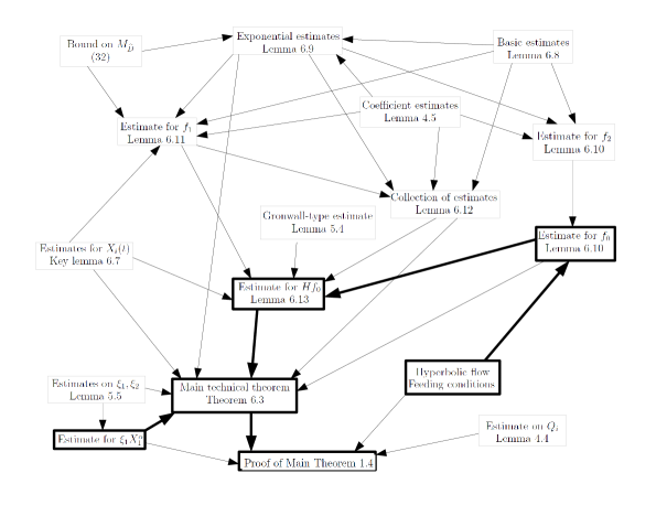
Figure 3. Map of Section 6.

Let $\omega$ be a given double-odd solution of the Euler equation that is in $C^{1}([0,\infty),C^{2}(\mathbb{T}))$. Moreover, let $\widehat{D}$ be a box depending on the parameters $\delta_{1},\delta_{2},\delta_{3}>0$ satisfying the conditions (17).

Suppose also that for the remainder of this section, (i)-(iv) from theorem 6.3 are satisfied. For abbreviation, we write in the following

$$M:=\max\{K,R\}.$$

We observe the following important fact: since $\delta_{1},\delta_{2},\delta_{3}\leq 1$,

(36) $$M_{\widehat{D}}(t)\leq M$$

holds.

We consider associated particle trajectories, which are the solutions of

(37) $$\dot{X}_{1}=-X_{1}Q_{1},\,\,\,\dot{X}_{2}=X_{2}Q_{2}.$$

More precisely, we define the particle trajectories as follows: for any $(x_{0},t_{0})\in\overline{D}\times[0,\infty)$ we take the maximal solution of $t\mapsto\mathbf{X}(t)$ of (37) which passes through $(x_{0},t_{0})$, and lies $\overline{D}$. $\mathbf{X}$ is defined on an interval $[T_{0},T_{e}]$ such that

1. $\mathbf{X}(t)\in\overline{D}$ for all $T_{0}\leq t\leq T_{e}$,

2. either $T_{0}=0$ or $T_{0}>0$, in which case necessarily $\mathbf{X}(T_{0})\in\partial D$,

3. $\mathbf{X}(T_{e})\in\partial D$.

Observe that $\mathbf{X}$ is given by

(38) $$\begin{split}X_{1}(t)&=X_{1}(T_{0})\exp\left(-\int_{T_{0}}^{t}Q_{1}(\mathbf{X}(s),s)~{}ds\right)\\ X_{2}(t)&=X_{2}(T_{0})\exp\left(\int_{T_{0}}^{t}Q_{2}(\mathbf{X}(s),s)~{}ds\right).\end{split}$$

We call $T_{0}$ the entry time and $T_{e}$ the exit time of a particle trajectory. $T_{0}=0$ if the particle starts in $\overline{D}$ for $t=0$.

The next proposition gives a upper bound for the time a particle can spend in the upper half of the box $D$, provided the flow is $\beta$-hyperbolic.

Proposition 6.4.

Suppose that the flow is $\beta$-hyperbolic in the box $D$ on the time interval $[0,T]$. Let $\mathbf{X}$ be a particle trajectory whose entry time $T_{0}$ is smaller than $T$.Then if $X_{2}(T_{0})\neq 0$ there is either a time $T_{1}$, $T_{e}>T_{1}\geq T_{0}$ such that

$$X_{2}(t)\geq\frac{1}{2}\delta_{2}\quad(t\in[T_{1},T])$$

or

$$X_{2}(t)\leq\frac{1}{2}\delta_{2}\quad(t\in[T_{0},T]).$$

If $T_{1}$ exists, we have the estimate

$$T_{e}-T_{1}\leq{\beta}^{-1}\log(2).$$

Proof.

The statement on the time $T_{1}$ follows directly form the fact that the flow is $\beta$-hyperbolic in the box. If $T_{1}$ exists, we have analogously to (38)

$$\delta_{2} =X_{2}(T_{e})=X_{2}(T_{1})\exp\left(\int_{T_{1}}^{T_{e}}Q_{2}~{}ds\right)\geq\frac{\delta_{2}}{2}\exp\left(\int_{T_{1}}^{T_{e}}Q_{2}~{}ds\right)\geq\frac{\delta_{2}}{2}\exp\left(\beta(T_{e}-T_{1})\right).$$

Solving for $T_{e}-T_{1}$ gives the result. ∎

Definition 6.5.

We call a function $g=g(\alpha,\beta,\boldsymbol{\delta},M)$ harmless generic factor it has the following property: There exists a $p_{0}>0$ such that for all $p\geq p_{0}$ and fixed $\alpha,\beta,M$

$$g(\alpha,\beta,\delta_{2}^{p},\delta_{2},M)$$

is bounded as $\delta_{2}\to 0$.

Remark 6.6.

For example, a function of the form

$$g=C(\alpha,\beta)\left[\delta_{2}^{\gamma_{3}}M(1+|\log\delta_{2}|)+\delta_{1}^{\gamma_{1}}{\delta_{2}}^{-\gamma_{2}}+1\right]^{\gamma_{4}}+C(\alpha,\beta,\gamma_{j})$$

($\gamma_{j}>0$) is a harmless generic factor, and $e^{g}$ is also a harmless generic factor if $g$ is one. When performing estimations, we shall often absorb harmless generic factors into one another, so the actual meaning of $g$ may change from line to line.

In our argument there will appear only finitely many different generic factors (although all denoted by $g$). To make the boundedness of them all work as $\delta_{2}\to 0$ we just pick a $p$ that is bigger than all the $p_{0}$ of all appearing generic factors.

Our goal will be to obtain estimates for the quantities $f_{0},f_{1},f_{2},v_{1},v_{2}$ along a single particle trajectory, up to the given time $T$, so that we can apply our ODE estimates from section 5. The crucial point is that our bounds depend not directly on $\omega,~{}T,~{}T_{e}$ but only on $\beta,\alpha,\mathbf{X}(T_{0})$. For the estimations below we often refer to a fixed particle trajectory with entry time $T_{0}$, along which we evaluate integrals over time of the quantities $Q_{1},Q_{2},c$ etc. To make the notation more compact, we often skip $\mathbf{X}$ in the arguments of the integrands, e.g. we write

$$\int_{T_{0}}^{t}|c|e^{-A}~{}ds=\int_{T_{0}}^{t}|c|e^{-A(s)}ds=\int_{T_{0}}^{t}|c(\mathbf{X}(s),s)|\exp\left(\int_{T_{0}}^{s}a(\mathbf{X}(\tau),\tau)~{}d\tau\right)~{}ds.$$

Lemma 6.7.

For any $t\leq T_{e}$,

$$X_{2}(T_{0})\leq\delta_{2}\exp\left(-\int_{T_{0}}^{t}Q_{2}(\mathbf{X}(s),s)~{}ds\right).$$

Proof.

Since the particle trajectory lies in $D$ for $t\in[T_{0},T_{e}]$,

$$\delta_{2}\geq X_{2}(t)=X_{2}(T_{0})\exp\left(\int_{T_{0}}^{t}Q_{2}~{}ds\right)$$

holds. ∎

Let $\phi:[0,\infty)\to[0,\infty)$ be a function with the properties

$$\phi(s)\leq 1-e^{-s}$$

and $\phi$ monotone nondecreasing on $[0,\infty)$, $\phi$ linear on $[0,s^{*}]$ and $\phi$ constant on $[s^{*},\infty)$ for some $s^{*}$. We fix such a function $\phi$ for the following.

Proposition 6.8.

Along a particle trajectory in a $\beta$-hyperbolic flow in $D$, we have the following for $t\in[T_{0},\min\{T_{e},T\}]$:

1. $$X_{1}(t) \leq\delta_{1}\exp\left(-\beta(t-T_{0})\right)$$

   $$X_{2}(t) \leq\delta_{2}\exp\left(-\beta(\min\{T_{e},T\}-t)\right),$$

2. $$d(\mathbf{X}(t))\geq\delta_{2}\phi\left(\int_{t}^{\min\{T_{e},T\}}Q_{2}~{}ds\right)\geq\delta_{2}\phi(\beta(\min\{T,T_{e}\}-t)),$$

3. Suppose $T_{1}$ from proposition 6.4 exists. Then the following holds for any $\gamma\in(0,1)$ and $t\in[T_{1},\min\{T_{e},T\}]$:

   $$\int_{T_{1}}^{t}d(\mathbf{X}(s))^{-1+\gamma}~{}ds\leq C(\gamma,\beta)\delta_{2}^{-1+\gamma},$$

   $$\int_{T_{1}}^{t}|\log d(\mathbf{X}(s))|~{}ds\leq C(\beta)|\log\delta_{2}|$$

   with $C(\beta),C(\gamma,\beta)$ independent of the trajectory.

Proof.

For (i), recall that under the assumption of $\beta$-hyperbolic flow, $Q_{2}\geq\beta$. From (38), we get

$$X_{2}(t)=X_{2}(T_{0})\exp\left(\int_{T_{0}}^{\min\{T_{e},T\}}Q_{2}~{}ds-\int_{t}^{\min\{T_{e},T\}}Q_{2}~{}ds\right)$$

$$\,\,\,=X_{2}(\min\{T_{e},T\})\exp\left(-\int_{t}^{\min\{T_{e},T\}}Q_{2}~{}ds\right)$$

(39) $$\,\,\,\leq\delta_{2}\exp\left(-\beta(\min\{T_{e},T\}-t)\right),$$

noting that $X_{2}(\min\{T_{e},T\})\leq\delta_{2}$. The bound for $X_{1}$ is analogous.

Now we show (ii). Recall that $d(\mathbf{X})=\delta_{2}-X_{2}(t)$. Hence by (39)

$$\delta_{2}-X_{2}(t) =\delta_{2}\left(1-\exp\left(-\int_{t}^{\min\{T_{e},T\}}Q_{2}~{}ds\right)\right)\geq\delta_{2}\phi\left(\int_{t}^{\min\{T_{e},T\}}Q_{2}~{}ds\right)$$

$$\geq\delta_{2}\phi\left(\beta(\min\{T_{e},T\}-t)\right).$$

(iii) We split the integrals by introducing the time $T^{*}$ defined as follows: $T^{*}$ is the maximum of all $s\in[T_{1},\min\{T_{e},T\}]$ such that

$$\phi(\beta(\min\{T_{e},T\}-s))=\phi(s^{*}).$$

If there are no such $s$, we set $T^{*}=T_{1}$. Thus we split the integrals in (iii) as follows:

$$\int_{T_{1}}^{t}=\int_{T_{1}}^{T^{*}}\ldots+\int_{T^{*}}^{t}\ldots$$

if $t\geq T^{*}$, otherwise we have only one integral from $T_{1}$ to $t$. We calculcate

$$\int_{T_{1}}^{T^{*}}d(\mathbf{X}(s))^{-1+\gamma}~{}ds \leq\delta_{2}^{-1+\gamma}\int_{T_{1}}^{T^{*}}\phi(\beta(\min\{T_{e},T\}-s))^{-1+\gamma}~{}ds$$

$$\leq\delta_{2}^{-1+\gamma}(T_{e}-T_{1})\phi(s^{*})^{-1+\gamma}\leq C(\beta,\gamma)\delta_{2}^{-1+\gamma}$$

$$\int_{T^{*}}^{t}d(\mathbf{X}(s))^{-1+\gamma}~{}ds \leq\delta_{2}^{-1+\gamma}\int_{T^{*}}^{t}\phi(\beta(\min\{T_{e},T\}-s))^{-1+\gamma}~{}ds$$

$$\lesssim\delta_{2}^{-1+\gamma}\beta^{-1+\gamma}\int_{T^{*}}^{t}(\min\{T_{e},T\}-s)^{-1+\gamma}~{}ds$$

$$\lesssim\delta_{2}^{-1+\gamma}\beta^{-1+\gamma}\int_{T_{1}}^{\min\{T_{e},T\}}(\min\{T_{e},T\}-s)^{-1+\gamma}~{}ds$$

$$\lesssim\delta_{2}^{-1+\gamma}\beta^{-1+\gamma}\int_{0}^{T_{e}-T_{1}}z^{-1+\gamma}~{}dz\lesssim\delta_{2}^{-1+\gamma}C(\beta,\gamma).$$

using (ii), Proposition 6.4 to estimate $T_{e}-T_{1}$ and the fact that $\phi$ is linear on $[0,s^{*}]$. The second integral is treated analogously. ∎

Lemma 6.9.

Along a particle trajectory, we have, for $T_{0}\leq t\leq\min\{T,T_{e}\}$,

$$e^{\pm A(t)} \leq g(\alpha,\beta,\boldsymbol{\delta},M)\exp\left(\pm\int_{T_{0}}^{t}Q_{2}(s)~{}ds\right),$$

$$\exp\left(\pm\int_{T_{0}}^{t}Q_{i}(s)~{}ds\right) \leq g(\alpha,\beta,\boldsymbol{\delta},M)\exp\left(\pm\int_{T_{0}}^{t}Q_{j}(s)~{}ds\right),\quad i,j=1,2$$

where $g(\alpha,\beta,\boldsymbol{\delta},M)$ are harmless generic factors depending only on the quantities indicated.

Proof.

We prove the first inequality of the Lemma, for the other we use similar arguments. Recall $a(t)=Q_{2}(t)+X_{2}(t)\partial_{x_{2}}Q_{2}(t)$, $A(t)=\int_{T_{0}}^{t}a(s)~{}ds$ and thus

$$\pm A(t)\leq\pm\int_{T_{0}}^{t}Q_{2}(s)~{}ds+\int_{T_{0}}^{t}|X_{2}(s)\partial_{x_{2}}Q_{2}(s)|~{}ds.$$

We now use Lemma 4.5 and (36):

$$\int_{T_{0}}^{t}|X_{2}(s)\partial_{x_{2}}Q_{2}(s)|~{}ds\leq C(\alpha)M\int_{T_{0}}^{\min\{T,T_{e}\}}X_{2}^{1-\alpha}(1+|\log d(\mathbf{X})|)~{}ds$$

$$+C(\alpha,\gamma)\int_{T_{0}}^{\min\{T,T_{e}\}}X_{2}^{1-\gamma}d(\mathbf{X})^{-1+\gamma}~{}ds.$$

Note that the interval of integration has been enlarged. With $T_{1}$ from proposition 6.4 we split the interval of integration into $[T_{0},T_{1}]$ and $[T_{1},\min\{T,T_{e}\}]$ provided $\min\{T,T_{e}\}\geq T_{1}$. The case $\min\{T,T_{e}\}<T_{1}$ is analogous.

In the part over $[T_{0},T_{1}]$, while $d(\mathbf{X})\geq\frac{1}{2}\delta_{2}$, we cannot control the length of the time interval, so we estimate as follows:

$$\int_{T_{0}}^{T_{1}}X_{2}^{1-\alpha}(1+|\log d(\mathbf{X})|) \leq\delta_{2}^{1-\alpha}\int_{T_{0}}^{T_{1}}e^{-(1-\alpha)\beta(\min\{T,T_{e}\}-s)}(C+|\log\delta_{2}|)~{}ds$$

$$\leq C\delta_{2}^{1-\alpha}|\log\delta_{2}|\int_{0}^{\infty}e^{-(1-\alpha)\beta z}~{}dz$$

$$\leq C(\alpha,\beta)\delta_{2}^{1-\alpha}|\log\delta_{2}|,$$

using part (i) of proposition 6.8 and $d(\mathbf{X}(s))\geq\frac{1}{2}\delta_{2}$ for $s\in[T_{0},T_{1}]$, and $\delta_{2}$ sufficiently small. In the part over $[T_{1},\min\{T,T_{e}\}]$ the length of the time interval is bounded but $|\log d(\mathbf{X})|$ is unbounded, so we proceed differently:

$$\int_{T_{1}}^{\min\{T,T_{e}\}}X_{2}^{1-\alpha}(1+|\log d(\mathbf{X})|) \leq\delta_{2}^{1-\alpha}\int_{T_{1}}^{\min\{T,T_{e}\}}|\log d(\mathbf{X})|~{}ds$$

$$\leq C(\beta)\delta_{2}^{1-\alpha}|\log\delta_{2}|.$$

using statement (iii) of Proposition 6.8 and $X_{2}\leq\delta_{2}$.

For the second integral involving $X_{2}^{1-\gamma}d(\mathbf{X})^{-1+\gamma}$, we note

$$\int_{T_{0}}^{T_{1}}X_{2}^{1-\gamma}d(\mathbf{X})^{-1+\gamma_{1}} \leq C(\gamma)\delta_{2}^{-1+\gamma}\int_{T_{0}}^{T_{1}}\left(\delta_{2}e^{-\beta(\min\{T,T_{e}\}-s)}\right)^{1-\gamma}ds$$

$$\leq C(\gamma,\beta)$$

$$\int_{T_{1}}^{\min\{T,T_{e}\}}X_{2}^{1-\gamma}d(\mathbf{X})^{-1+\gamma} \leq\delta_{2}^{1-\gamma}\int_{T_{1}}^{\min\{T,T_{e}\}}d(\mathbf{X})^{-1+\gamma}$$

$$\leq C(\gamma,\beta)$$

by proposition 6.8, (i) and (iii) and moreover using $X_{2}\leq\delta_{2}$. This yields finally

$$\int_{T_{0}}^{t}|X_{2}(s)\partial_{x_{2}}Q_{2}(s)|~{}ds\leq[C(\alpha,\beta)M\delta_{2}^{1-\alpha}|\log\delta_{2}|+C(\gamma,\beta)]$$

implying the result, since the term in square brackets is a harmless generic factor.

To prove the second inequality, we use (the velocity field is divergence-free)

$$Q_{1}(t)+X_{1}(t)\partial_{x_{1}}Q_{1}(t)=Q_{2}(t)+X_{2}(t)\partial_{x_{2}}Q_{2}(t)$$

implying $|Q_{i}|\leq|Q_{j}|+\sum_{k=1}^{2}|x_{k}\partial_{x_{k}}Q_{k}|$. The expressions involving $x_{k}\partial_{x_{k}}Q_{k}$ are estimated as before. ∎

6.3. Estimates for $f_{0},f_{1},f_{2},v_{1},v_{2}$ and $Hf_{0}$.

Lemma 6.10.

The following estimates hold for $T_{0}\leq t\leq\min\{T,T_{e}\}$:

(40) $$f_{2}(t) \leq g(\alpha,\beta,\boldsymbol{\delta},M)X_{2}(T_{0})^{1-\alpha},$$

$$f_{0}(t) \leq R\,g(\alpha,\beta,\boldsymbol{\delta},M)X_{2}(T_{0})^{1-\alpha}.$$

Proof.

We write $g=g(\alpha,\beta,\boldsymbol{\delta},M)$ for any occuring harmless factor. Using Lemma 4.5 with $\gamma_{1}=\gamma_{2}=\frac{\alpha}{2}$,

$$f_{2}(t) =\int_{T_{0}}^{t}e^{-A}|c|\lesssim M\int_{T_{0}}^{\min\{T,T_{e}\}}e^{-A}X_{2}^{1-\alpha}~{}ds$$

$$\,\,+C(\alpha)\int_{T_{0}}^{\min\{T,T_{e}\}}e^{-A}X_{2}^{1-\alpha}X_{1}^{\alpha/2}d(\mathbf{X})^{-1+\alpha/2}ds.$$

Observe first that by Lemma 6.9 $e^{-A(s)}$ is estimated by $\exp\left(-\int_{T_{0}}^{s}Q_{2}~{}d\tau\right)$ and thus using $Q_{2}\geq\beta$ again we get

(41) $$e^{-A}X_{2}(s)^{1-\alpha} \leq gX_{2}(T_{0})^{1-\alpha}\exp\left(-\alpha\int_{T_{0}}^{s}Q_{2}~{}d\tau\right)\leq gX_{2}(T_{0})^{1-\alpha}\exp\left(-\alpha\beta(s-T_{0})\right).$$

Employing (41) to estimate the integral containing $e^{A}X_{2}^{1-\alpha}$ yields:

$$\int_{T_{0}}^{\min\{T,T_{e}\}}\!\!\!\!\!e^{-A}X_{2}^{1-\alpha}ds \leq g\,X_{2}(T_{0})^{1-\alpha}\int_{T_{0}}^{\infty}e^{-\alpha\beta(s-T_{0})}ds\leq g\,X_{2}(T_{0})^{1-\alpha}C(\alpha,\beta).$$

For the integral containing $e^{-A}X_{2}^{1-\alpha}X_{1}^{\alpha/2}d(\mathbf{X})^{1-\alpha/2}$, we use (41) again and estimate

$$\int_{T_{0}}^{\min\{T,T_{e}\}}\!\!\!\!\!e^{-A}X_{2}^{1-\alpha}X_{1}^{\alpha/2}d(\mathbf{X})^{1-\alpha/2}ds\leq gX_{2}(T_{0})^{1-\alpha}\delta_{1}^{\alpha/2}\int_{T_{0}}^{\min\{T,T_{e}\}}\!\!\!\!\!e^{-\alpha\beta(s-T_{0})}d(\mathbf{X})^{-1+\alpha/2}ds.$$

As in the proof of Lemma 6.9, we split the interval of integration into $[T_{0},T_{1}]$ and $[T_{1},\min\{T,T_{e}\}]$ in case $T_{1}\leq\min\{T,T_{e}\}$, obtaining

(42) $$\int_{T_{0}}^{T_{1}}e^{-\alpha\beta(s-T_{0})}d(\mathbf{X})^{-1+\alpha/2}~{}ds \lesssim\delta_{2}^{-1+\alpha/2},$$

(43) $$\int_{T_{1}}^{\min\{T,T_{e}\}}e^{-\alpha\beta(s-T_{0})}d(\mathbf{X})^{-1+\alpha/2}~{}ds \lesssim\int_{T_{1}}^{\min\{T,T_{e}\}}d(\mathbf{X})^{-1+\alpha/2}~{}ds\lesssim\delta_{2}^{-1+\alpha/2}$$

where we have used $d(\mathbf{X})\geq\frac{1}{2}\delta_{2}$ for (42) and $e^{-\alpha\beta(s-T_{0})}\leq 1$ and Proposition 6.8 for (43). The case $T_{1}\geq\min\{T,T_{e}\}$ is covered by (42). To estimate $f_{0}$, we use that the feeding condition holds and that assumption (iii) from Theorem 6.3 holds. This gives

$$|\xi_{1}(T_{0})| =|\partial_{x_{1}}\omega(\mathbf{X}(T_{0}),T_{0})|\leq RX_{2}(T_{0})^{1-\alpha},$$

$$|\xi_{2}(T_{0})| =|\partial_{x_{2}}\omega(\mathbf{X}(T_{0}),T_{0})|\leq R$$

for both of the cases $T_{0}=0$ (particle starts in $D$) and $T_{0}>0$ (particle starts in or crosses the feeding zone before entering $D$). Now use the definition of $f_{0}$ and the estimate (40) for $f_{2}$. ∎

Lemma 6.11.

For $T_{0}\leq t\leq\min\{T,T_{e}\}$,

$$f_{1}(t) \leq g(\alpha,\beta,\boldsymbol{\delta},M)\delta_{1}^{1-\alpha}\delta_{2}^{\alpha}e^{\alpha\int_{T_{0}}^{t}Q_{2}\,ds}$$

with a harmless generic factor $g$ depending on the quantities indicated.

Proof.

We abbreviate again $g=g(\alpha,\beta,\boldsymbol{\delta},M)$. First we claim that for sufficiently small $\delta_{2}$

(44) $$\int_{T_{0}}^{t}e^{2A}|b|~{}ds \leq g\,X_{1}(T_{0})^{1-\alpha}\left[M|\log\delta_{2}|+\delta_{1}^{\frac{\alpha}{2}}{\delta_{2}}^{-1+\frac{\alpha}{2}}\right]e^{(1+\alpha)\int_{T_{0}}^{t}Q_{2}\,ds}.$$

We treat the case $T_{1}\leq t\leq\min\{T,T_{e}\}$. Using Lemma 4.5 with $\gamma=\frac{\alpha}{2}$, and Lemma 6.9 we get

$$e^{2A}|b| \leq e^{2A}X_{1}^{1-\alpha}[M_{\widehat{D}}(t)(1+|\log d(\mathbf{X})|)+X_{1}^{\frac{\alpha}{2}}d(\mathbf{X})^{-1+\frac{\alpha}{2}}]$$

$$\leq g\,e^{(1+\alpha)\int_{T_{0}}^{s}Q_{1}ds}\,X_{1}(T_{0})^{1-\alpha}[M(1+|\log d(\mathbf{X})|)+\delta_{1}^{\frac{\alpha}{2}}d(\mathbf{X})^{-1+\frac{\alpha}{2}}].$$

Also recall that $M_{\widehat{D}}(t)\leq M$. To integrate this bound from $T_{0}$ to $t$ we split into two integrals from $T_{0}$ to $T_{1}$ and $T_{1}$ to $t$. For $t\in[T_{0},T_{1}]$ we can estimate the factor in square brackets independent of $t$ using $d(\mathbf{X})\geq\frac{1}{2}\delta_{2}$:

$$g\,X_{1}(T_{0})^{1-\alpha}[M(1+|\log\delta_{2}|)+\delta_{1}^{\frac{\alpha}{2}}\delta_{2}^{-1+\frac{\alpha}{2}}]\int_{T_{0}}^{T_{1}}e^{(1+\alpha)\int_{T_{0}}^{s}Q_{1}d\tau}~{}ds.$$

The remaining integral can be estimated as follows:

$$\int_{T_{0}}^{T_{1}}e^{(1+\alpha)\int_{T_{0}}^{s}Q_{1}d\tau}~{}ds \leq\int_{T_{0}}^{t}\frac{Q_{1}}{Q_{1}}e^{(1+\alpha)\int_{T_{0}}^{s}Q_{1}d\tau}~{}ds\leq\beta^{-1}(1+\alpha)^{-1}\left.e^{(1+\alpha)\int_{T_{0}}^{s}Q_{1}d\tau}\right|_{s=T_{0}}^{s=t}$$

$$\lesssim e^{(1+\alpha)\int_{T_{0}}^{t}Q_{1}d\tau}.$$

Hence for sufficiently small $\delta_{2}$

$$\int_{T_{0}}^{T_{1}}e^{2A}|b|~{}ds \lesssim g\,X_{1}(T_{0})^{1-\alpha}[M|\log\delta_{2}|+\delta_{1}^{\frac{\alpha}{2}}\delta_{2}^{-1+\frac{\alpha}{2}}]e^{(1+\alpha)\int_{T_{0}}^{T_{1}}Q_{1}}.$$

For the remaining part $\int_{T_{1}}^{t}e^{2A}|b|~{}ds$, we use Proposition 6.8 again, and find the bound for small $\delta_{2}$

$$g\,X_{1}(T_{0})^{1-\alpha}\int_{T_{1}}^{t}e^{(1+\alpha)\int_{T_{0}}^{s}Q_{1}ds}[M(1+|\log d(\mathbf{X})|)+\delta_{1}^{\frac{\alpha}{2}}d(\mathbf{X})^{-1+\frac{\alpha}{2}}]~{}ds$$

$$\leq g\,e^{(1+\alpha)\int_{T_{0}}^{t}Q_{1}ds}X_{1}(T_{0})^{1-\alpha}\int_{T_{1}}^{t}[M(1+|\log d(\mathbf{X})|)+\delta_{1}^{\frac{\alpha}{2}}d(\mathbf{X})^{-1+\frac{\alpha}{2}}]~{}ds$$

$$\,\,\lesssim g\,X_{1}(T_{0})^{1-\alpha}[M|\log\delta_{2}|+\delta_{1}^{\alpha/2}\delta_{2}^{-1+\alpha/2}]e^{(1+\alpha)\int_{T_{0}}^{t}Q_{1}ds}.$$

Using the second estimate from Lemma 6.9 the claim follows for the case $T_{1}\leq t\leq\min\{T,T_{e}\}$. The calculation for $t\leq T_{1}$ is similar (and slightly simpler).

Next, using again Lemma 4.5 with $\gamma_{1}=\gamma_{2}=\alpha/2$ and Lemma 6.9,

$$e^{-A}|c| \leq e^{-A}X_{2}^{1-\alpha}[M+X_{1}^{\alpha/2}d(\mathbf{X})^{-1+\alpha/2}]$$

$$\leq g\,e^{-\alpha\int_{T_{0}}^{t}Q_{2}~{}ds}X_{2}(T_{0})^{1-\alpha}\left[M+\delta_{1}^{\alpha/2}d(\mathbf{X})^{-1+\alpha/2}\right].$$

Hence

$$\int_{T_{0}}^{t}e^{-A}|c|\int_{T_{0}}^{s}e^{2A}|b| \lesssim g\,X_{2}(T_{0})^{1-\alpha}X_{1}(T_{0})^{1-\alpha}\left[M|\log\delta_{2}|+\delta_{1}^{\alpha/2}{\delta_{2}}^{-1+\alpha/2}\right]$$

$$\qquad\times\int_{T_{0}}^{t}e^{\int_{T_{0}}^{s}Q_{2}\,d\tau}[M+\delta_{1}^{\alpha/2}d(\mathbf{X})^{-1+\alpha/2}]~{}ds.$$

We continue to estimate the last integral:

$$\int_{T_{0}}^{t}e^{\int_{T_{0}}^{s}Q_{2}\,d\tau}[M+\delta_{1}^{\alpha/2}d(\mathbf{X})^{-1+\alpha/2}]~{}ds$$

$$= \,M\int_{T_{0}}^{t}e^{\int_{T_{0}}^{s}Q_{2}\,d\tau}ds+\int_{T_{0}}^{t}e^{\int_{T_{0}}^{s}Q_{2}\,d\tau}\delta_{1}^{\alpha/2}d(\mathbf{X})^{-1+\alpha/2}~{}ds$$

$$\leq \,M\int_{T_{0}}^{t}\frac{Q_{2}}{Q_{2}}e^{\int_{T_{0}}^{s}Q_{2}\,d\tau}ds+e^{\int_{T_{0}}^{t}Q_{2}\,d\tau}\delta_{1}^{\alpha/2}\int_{T_{0}}^{t}d(\mathbf{X})^{-1+\alpha/2}~{}ds$$

$$\lesssim \,e^{\int_{T_{0}}^{t}Q_{2}\,ds}\left[M+\delta_{1}^{\alpha/2}\delta_{2}^{-1+\alpha/2}\right]$$

where we used the familiar splitting at $T_{1}$. Thus, finally we get

$$\int_{T_{0}}^{t}e^{-A}|c|\int_{T_{0}}^{s}e^{2A}|b| \lesssim g\,X_{1}(T_{0})^{1-\alpha}\left[M|\log\delta_{2}|+\delta_{1}^{\alpha/2}{\delta_{2}}^{-1+\alpha/2}\right]$$

$$\qquad\times[M+\delta_{1}^{\alpha/2}\delta_{2}^{-1+\alpha/2}]e^{\int_{T_{0}}^{t}Q_{2}\,ds}X_{2}(T_{0})^{1-\alpha}.$$

It remains to apply key Lemma 6.7 to estimate the factor $e^{\int_{T_{0}}^{t}Q_{2}\,ds}X_{2}(T_{0})^{1-\alpha}$, which is less than

$$\delta_{2}^{1-\alpha}e^{\int_{T_{0}}^{t}Q_{2}\,ds}e^{-(1-\alpha)\int_{T_{0}}^{t}Q_{2}\,ds}\leq\delta_{2}^{1-\alpha}e^{\alpha\int_{T_{0}}^{t}Q_{2}\,ds}=\delta_{2}^{1-2\alpha}\delta_{2}^{\alpha}e^{\alpha\int_{T_{0}}^{t}Q_{2}\,ds}.$$

Now observe that the expression $\left[M|\log\delta_{2}|+\delta_{1}^{\alpha/2}{\delta_{2}}^{-1+\alpha/2}\right][M+\delta_{1}^{\alpha/2}\delta_{2}^{-1+\alpha/2}]\delta_{2}^{1-2\alpha}$ is a harmless factor since $\alpha<1/4$.

∎

Lemma 6.12.

For sufficiently small $\delta_{2}$ and $t\in[T_{0},\min\{T,T_{e}\}]$ we have the following inequalities.

(45) $$v_{1}(t)\leq g\left[Q_{2}+MX_{2}^{1-\alpha}|\log d(\mathbf{X})|+\delta_{2}^{1-\alpha}d(\mathbf{X})^{-1+\alpha}\right]e^{-\int_{T_{0}}^{t}Q_{2}\,ds},$$

(46) $$v_{2}(t)\leq g\,X_{1}(T_{0})^{1-\alpha}\left[M|\log d(\mathbf{X})|+\delta_{1}^{\alpha/2}d(\mathbf{X})^{-1+\alpha/2}\right]e^{\alpha\int_{T_{0}}^{t}Q_{2}\,ds},$$

(47) $$\int_{T_{0}}^{t}v_{1}e^{\alpha\int_{T_{0}}^{s}Q_{2}~{}d\tau}~{}ds\leq g$$

(48) $$\int_{T_{0}}^{t}v_{2}~{}ds\leq g\,e^{\alpha\int_{T_{0}}^{t}Q_{2}\,ds}$$

(49) $$\int_{T_{0}}^{t}v_{2}e^{\alpha\int_{T_{0}}^{s}Q_{2}\,d\tau}\,ds\leq g\,e^{2\alpha\int_{T_{0}}^{t}Q_{2}\,ds},$$

(50) $$\int_{T_{0}}^{t}v_{1}f_{1}~{}ds\leq g\,\delta_{1}^{1-\alpha}\delta_{2}^{\alpha},$$

(51) $$\int_{T_{0}}^{t}v_{2}f_{1}~{}ds\leq g\,\delta_{1}^{1-\alpha}\delta_{2}^{\alpha/2}X_{1}(T_{0})^{1-\alpha}e^{2\alpha\int_{T_{0}}^{t}Q_{2}~{}d\tau},$$

(52) $$\int_{T_{0}}^{t}v_{1}f_{2}~{}ds\leq gX_{2}(T_{0})^{1-\alpha},$$

where $g=g(\alpha,\beta,\boldsymbol{\delta},M)$ is a harmless factor.

Proof.

The estimates (45)-(48) follow from Lemma 4.5, Lemma 6.9, Proposition 6.8 and the usual splitting of the interval of integration into $[T_{0},T_{1}]$ and $[T_{1},\min\{T,T_{e}\}]$ . (49) follows easily from (48) and Lemma 6.9.

Using Lemma 6.11 and Lemma 4.5 we get

$$v_{1}f_{1}(s) \leq g\,\delta_{1}^{1-\alpha}\delta_{2}^{\alpha}\left[Q_{2}+MX_{2}^{1-\alpha}|\log d(\mathbf{X})|+\delta_{2}^{1-\alpha}d(\mathbf{X})^{-1+\alpha}\right]e^{(-1+\alpha)\int_{T_{0}}^{s}Q_{2}\,d\tau}.$$

Note how the exponential growth of the factor $f_{1}$ was cancelled by the exponential factor in $v_{1}$. By integrating, we get:

$$\int_{T_{0}}^{t}v_{1}f_{1}~{}ds \leq g\,\delta_{1}^{1-\alpha}\delta_{2}^{\alpha}\int\limits_{T_{0}}^{t}e^{(-1+\alpha)\int_{T_{0}}^{s}Q_{2}~{}d\tau}\left[Q_{2}+M\delta_{2}^{1-\alpha}|\log d(\mathbf{X})|+\delta_{2}^{1-\alpha}d(\mathbf{X})^{-1+\alpha}\right]~{}ds$$

$$\leq g\,\delta_{1}^{1-\alpha}\delta_{2}^{\alpha}\left[M\delta_{2}^{1-\alpha}|\log\delta_{2}|+1\right]$$

giving (50) since the factor in square brackets is harmless and can be absorbed into $g$.

Proceeding analogously to prove (51) we find

$$v_{2}f_{1}(s) \leq\,g\delta_{1}^{1-\alpha}\delta_{2}^{\alpha}X_{1}(T_{0})^{1-\alpha}e^{2\alpha\int_{T_{0}}^{s}Q_{2}~{}d\tau}\left[M|\log d(\mathbf{X})|+\delta_{1}^{\alpha/2}d(\mathbf{X})^{-1+\alpha/2}\right]$$

which after integration from $T_{0}$ to $t$ can be estimated as follows:

$$\int_{T_{0}}^{t}v_{2}f_{1}~{}ds \leq g\,\delta_{1}^{1-\alpha}\delta_{2}^{\alpha}X_{1}(T_{0})^{1-\alpha}e^{2\alpha\int_{T_{0}}^{s}Q_{2}~{}d\tau}\left[M|\log\delta_{2}|+\delta_{1}^{\alpha/2}\delta_{2}^{-1+\alpha/2}\right]$$

$$\leq g\,\delta_{1}^{1-\alpha}\delta_{2}^{\alpha/2}X_{1}(T_{0})^{1-\alpha}e^{2\alpha\int_{T_{0}}^{t}Q_{2}~{}d\tau}\left[M\delta_{2}^{\alpha/2}|\log\delta_{2}|+\delta_{1}^{\alpha/2}\delta_{2}\right].$$

Again the factor in square brackets can be absorbed into $g$ giving (51).

(52) is derived using the same techniques.

∎

Lemma 6.13.

Along a particle trajectory, for $T_{0}\leq t\leq\min\{T,T_{e}\}$,

(53) $$(Hf_{0})(t) \leq g\|f_{0}\|_{\infty}(t)e^{\alpha\int_{T_{0}}^{t}Q_{2}~{}ds}$$

holds, where $\|f_{0}\|_{\infty}(t)=\sup\{|f_{0}(s)|\,:\,s\in[T_{0},t]\}$.

Proof.

Using Lemmas 6.11, 6.12, we get

(54) $$f_{0}+f_{1}\exp\left(\int_{T_{0}}^{t}v_{1}f_{1}\right)\int_{T_{0}}^{t}v_{1}f_{0} \leq g\,\|f_{0}\|_{\infty}(t)e^{\alpha\int_{T_{0}}^{t}Q_{2}\,ds}.$$

Recall that products and exponentials of harmless factors are harmless, too.

Next, using Lemma 6.10, 6.11 and 6.12

$$f_{2}+f_{1}\exp\left(\int_{T_{0}}^{t}v_{1}f_{1}\right)\int_{T_{0}}^{t}v_{1}f_{2} \leq g\,X_{2}(T_{0})^{1-\alpha}e^{\alpha\int_{T_{0}}^{t}Q_{2}~{}ds}$$

$$=g\,X_{2}(T_{0})^{1-2\alpha}X_{2}(T_{0})^{\alpha}e^{\alpha\int_{T_{0}}^{t}Q_{2}~{}ds}$$

$$\leq g\,X_{2}(T_{0})^{1-2\alpha}\delta_{2}^{\alpha}$$

with the key Lemma 6.7 in the last step to cancel of $e^{\alpha\int_{T_{0}}^{t}Q_{2}~{}ds}$ using the factor $X_{2}(T_{0})^{\alpha}$.

So for $v_{2}\left[f_{2}+f_{1}\exp\left(\int_{T_{0}}^{t}v_{1}f_{1}\right)\int_{T_{0}}^{t}v_{1}f_{2}\right]$ we obtain the upper bound

$$v_{2}gX_{2}(T_{0})^{1-2\alpha}\delta_{2}^{\alpha} \leq g\,e^{\alpha\int_{T_{0}}^{t}Q_{2}}X_{2}(T_{0})^{1-2\alpha}\delta_{2}^{\alpha}X_{1}(T_{0})^{1-\alpha}\left[M|\log d(\mathbf{X})|+\delta_{1}^{\alpha/2}d(\mathbf{X})^{-1+\alpha/2}\right]$$

$$\leq g\,\delta_{2}^{2\alpha}X_{2}(T_{0})^{1-3\alpha}\delta_{1}^{1-\alpha}\left[M|\log d(\mathbf{X})|+\delta_{1}^{\alpha/2}d(\mathbf{X})^{-1+\alpha/2}\right]$$

using the key Lemma 6.7 again to cancel $e^{\alpha\int_{T_{0}}^{t}Q_{2}}$. Thus we see that

$$\exp\left(\int_{T_{0}}^{t}v_{2}\left[f_{2}+f_{1}\exp\left(\int_{T_{0}}^{s}v_{1}f_{1}\right)\int_{T_{0}}^{s}v_{1}f_{2}\right]\right)\leq g$$

Finally, by (54) and Lemma 6.12

$$\int_{T_{0}}^{t}v_{2}\left[f_{0}+f_{1}\exp\left(\int_{T_{0}}^{s}v_{1}f_{1}\right)\int_{T_{0}}^{s}v_{1}f_{0}\right]\leq$$

$$\,\,g\|f_{0}\|_{\infty}(t)\int_{T_{0}}^{t}v_{2}e^{\alpha\int_{T_{0}}^{s}Q_{2}\,d\tau}ds\leq g\|f_{0}\|_{\infty}(t)e^{2\alpha\int_{T_{0}}^{t}Q_{2}\,ds}.$$

Thus, in total we get

$$f_{0}+f_{1}\exp\left(\int_{T_{0}}^{t}v_{1}f_{1}\right)\int_{T_{0}}^{t}v_{1}f_{0} \leq g\|f_{0}\|_{\infty}(t)e^{\alpha\int_{T_{0}}^{t}Q_{2}\,ds}$$

(55) $$f_{2}+f_{1}\exp\left(\int_{T_{0}}^{t}v_{1}f_{1}\right)\int_{T_{0}}^{t}v_{1}f_{2} \leq gX_{2}(T_{0})^{1-2\alpha}\delta_{2}^{\alpha}$$

(56) $$\exp\left(\int_{T_{0}}^{t}v_{2}\left[f_{2}+f_{1}\exp\left(\int_{T_{0}}^{s}v_{1}f_{1}\right)\int_{T_{0}}^{s}v_{1}f_{2}\right]\right) \leq g$$

(57) $$\int_{T_{0}}^{t}v_{2}\left[f_{0}+f_{1}\exp\left(\int_{T_{0}}^{s}v_{1}f_{1}\right)\int_{T_{0}}^{s}v_{1}f_{0}\right] \leq g\|f_{0}\|_{\infty}(t)e^{2\alpha\int_{T_{0}}^{t}Q_{2}~{}ds}.$$

Note that

$$\eqref{H0part2}\times\eqref{H0part4}\leq g\,X_{2}(T_{0})^{1-4\alpha}\delta_{2}^{4\alpha}\|f_{0}\|_{\infty}(t)\leq g$$

using again the key Lemma to get rid of the factor $e^{2\alpha\int_{T_{0}}^{t}Q_{2}}$, and in the very last step we used $\alpha\in(0,1/4)$ and Lemma 6.10. Combining the inequalities (55)-(57) gives

$$\left(f_{2}+f_{1}\exp\left(\int_{T_{0}}^{t}v_{1}f_{1}\right)\int_{T_{0}}^{t}v_{1}f_{2}\right)$$

$$\times\exp\left(\int_{T_{0}}^{t}v_{2}\left[f_{2}+f_{1}\exp\left(\int_{T_{0}}^{s}v_{1}f_{1}\right)\int_{T_{0}}^{t}v_{1}f_{2}\right]\right)$$

$$\times\int_{T_{0}}^{t}v_{2}\left[f_{0}+f_{1}\exp\left(\int_{T_{0}}^{s}v_{1}f_{1}\right)\int_{T_{0}}^{t}v_{1}f_{0}\right]$$

$$\leq gX_{2}(T_{0})^{1-4\alpha}\delta_{2}^{4\alpha}\|f_{0}\|_{\infty}(t)\leq g\|f_{0}\|_{\infty}(t)$$

In view of (32), (53) now follows. ∎

6.4. Proof of the main technical theorem

Proof of theorem 6.3.

At time $t=T$, any $x\in D$ is occupied by a particle, i.e. $x=\mathbf{X}(T)$ for some particle trajectory. Let us write

$$\partial_{x_{j}}\omega(\mathbf{X}(t),t)=\xi_{j}(t)$$

along that particle trajectory, and so by (35),

$$|\xi_{1}(t)| \leq(Hf_{0})(t)+e^{A}\int_{T_{0}}^{t}|a|e^{-A}(Hf_{0})(s)~{}ds=(Hf_{0})(t)+e^{A}\int_{T_{0}}^{t}v_{1}(Hf_{0})(s)~{}ds.$$

First note that by Lemmas 6.13, 6.10, 6.12 and 6.9

$$e^{A}\int_{T_{0}}^{t}v_{1}(s)(Hf_{0})(s)~{}ds \leq e^{A}g\,\|f_{0}\|_{\infty}(t)\int_{T_{0}}^{t}v_{1}e^{\alpha\int_{T_{0}}^{s}Q_{2}~{}d\tau}~{}ds\leq g\,RX_{2}(T_{0})^{1-\alpha}e^{A}$$

$$\leq g\,Re^{-(1-\alpha)\int_{T_{0}}^{t}Q_{2}~{}ds}e^{\int_{T_{0}}^{t}Q_{2}~{}ds}\leq g\,Re^{\alpha\int_{T_{0}}^{t}Q_{2}~{}ds}.$$

Moreover again by Lemmas 6.13, 6.10

$$(Hf_{0})(t) \leq g\,Re^{\alpha\int_{T_{0}}^{t}Q_{2}~{}ds}.$$

This results in

(58) $$|\xi_{1}(t)| \leq g\,Re^{\alpha\int_{T_{0}}^{t}Q_{2}~{}ds}.$$

Next we estimate $|\xi_{1}(t)|X_{1}(t)^{\alpha}$. First we use (58) and insert $X_{1}(t)$ from (38). Then Lemma 6.9 allows us to replace $Q_{1}$ by $Q_{2}$ in the one of the arguments of the exponential function, so we get the estimate

(59) $$\begin{split}|\xi_{1}(t)|X_{1}(t)^{\alpha}&\leq g\,RX_{1}(t)^{\alpha}e^{\alpha\int_{T_{0}}^{t}Q_{1}~{}ds}\leq g\,R\delta_{1}^{\alpha}e^{-\alpha\int_{T_{0}}^{t}Q_{1}~{}ds}e^{\alpha\int_{T_{0}}^{t}Q_{2}~{}ds}\\ &\leq g\,R\delta_{1}^{\alpha}e^{-\alpha\int_{T_{0}}^{t}Q_{2}~{}ds}e^{\alpha\int_{T_{0}}^{t}Q_{2}~{}ds}\leq g\,R\delta_{2}^{\alpha}\end{split}$$

since $\delta_{1}<\delta_{2}$. In fact, this was the most critical estimate in the whole proof of the main result, since the dangerous factor $e^{A}$ was barely cancelled.

We now derive a similar estimate for $|\xi_{2}(t)|X_{2}(t)^{\alpha}$. From the second line of (35) and the assumptions on initial conditions,

(60) $$|\xi_{2}(t)| \leq Re^{-A}+e^{-A}\int_{T_{0}}^{t}v_{2}\,Hf_{0}~{}ds+e^{-A}\int_{T_{0}}^{t}e^{2A}|b|\int_{T_{0}}^{s}v_{1}\,Hf_{0}~{}ds.$$

By Lemma 6.13 and 6.10 $Hf_{0}(s)$ has the upper bound

$$R\,g\,X_{2}(T_{0})^{1-\alpha}e^{\alpha\int_{T_{0}}^{s}Q_{2}~{}d\tau}.$$

Therefore the second summand can be estimated as follows

$$e^{-A}\int_{T_{0}}^{t}v_{2}\,Hf_{0}~{}ds \leq e^{-A}R\,g\,\int_{T_{0}}^{t}v_{2}e^{\alpha\int_{T_{0}}^{s}Q_{2}~{}d\tau}~{}ds\leq R\,g\,e^{-A}e^{2\alpha\int_{T_{0}}^{t}Q_{2}~{}ds}$$

$$\leq R\,g\,e^{(-1+2\alpha)\int_{T_{0}}^{t}Q_{2}~{}ds}\leq g\,R,$$

where we also used $X_{2}(T_{0})\leq\delta_{2}$, (49), Lemma 6.9 and $\alpha<1/4$.

For the third summand of (60) we use the upper bound for $Hf_{0}$ again:

$$e^{-A}\int_{T_{0}}^{t}e^{2A}|b|\int_{T_{0}}^{s}v_{1}\,Hf_{0}~{}ds \leq g\,R\,X_{2}(T_{0})^{1-\alpha}e^{-A}\int_{T_{0}}^{t}e^{2A}|b|\int_{T_{0}}^{s}v_{1}\,e^{\alpha\int_{T_{0}}^{\tau}Q_{2}~{}d\zeta}~{}d\tau~{}ds$$

$$\leq g\,R\,\delta_{2}^{1-\alpha}e^{-A}\int_{T_{0}}^{t}e^{2A}|b|~{}ds.$$

In the last estimate (47) was used. Now note that by (44)

$$\int_{T_{0}}^{t}e^{2A}|b|~{}ds \leq g\,e^{(1+\alpha)\int_{T_{0}}^{t}Q_{2}~{}ds}.$$

After combining this with the $e^{-A}$ factor we see that we can bound the third summand by $g\,R$, i.e. $|\xi_{2}(t)|\leq g\,R$. This means that

(61) $$|\xi_{2}(t)|X_{2}^{\alpha}\leq gR\delta_{2}^{\alpha}.$$

The inequalities (61) and (59) imply

$$M_{D}(T)\leq g(\alpha,\beta,\boldsymbol{\delta},M)R\delta_{2}^{\alpha}+\|\omega\|_{\infty}=:\mathcal{N}(R,\alpha,\beta,\boldsymbol{\delta},M).$$

It remains to show that $\mathcal{N}$ is a harmless nonlinearity. Therefore, let $\alpha,\beta,R$ be given. Recall that $g$ has the property that $g(\alpha,\beta,\delta_{2}^{p},\delta_{2},R)$ is bounded as $\delta_{2}\to 0$ for all $p>p_{0}$ with some $p_{0}>0$. Hence

$$g(\alpha,\beta,\delta_{2}^{p},\delta_{2},R)R\delta_{2}^{\alpha}+\|\omega\|_{\infty}<R$$

for sufficiently small $\delta_{2}>0$ and $R>\|\omega\|_{\infty}$. ∎

7. Proof of the main result

Proof of Theorem 1.4.

Let $\alpha\in(0,\frac{1}{4})$, $0<\delta_{3}<1/2$ and $R>\|\omega\|_{\infty}$ be a given nonnegative number. Fix small positive $\delta_{1},\delta_{2}$ such that the following set of inequalities hold true:

(62) $$\delta_{1},\delta_{2}\leq\rho,~{}\beta_{0}-A|\boldsymbol{\delta}|^{1-\alpha}R\geq\frac{1}{2}\beta_{0}.$$

(63) $$M_{D}(0)<R,~{}\left|\frac{\partial\omega_{0}(x)}{\partial x_{1}}\right|\leq Rx_{2}^{1-\alpha},~{}\left|\frac{\partial\omega_{0}(x)}{\partial x_{2}}\right|\leq R\quad(x\in D)$$

where $A,\beta_{0},\rho$ are the numbers from the Definition 1.2 of the hyperbolicity of the flow. Note that the box can be chosen so small that that (63) holds. This a consequence of $\frac{\partial\omega_{0}}{\partial x_{2}}(0,x_{2})=\frac{\partial\omega_{0}}{\partial x_{1}}(x_{1},0)=0$ and the $C^{2}$-smoothness of $\omega_{0}$.

Claim: If the box $\widehat{D}$ satisfies the controlled feeding conditions with parameter $R$, then we have the bound

(64) $$M_{D}(t)\leq R\quad(t\in[0,\infty)).$$

Assume (64) is not true for all times, i.e. there is a time $\widetilde{T}$ such that $M_{D}(\widetilde{T})>R$. Since the solution $\omega$ is sufficiently smooth in time by assumption, $M_{D}(t)$ is a continuous function of $t$. Because $M_{D}(0)<R$, by the intermediate value theorem, there exists a time $T\in(0,\widetilde{T})$ such that $M_{D}(t)<R$ holds on $[0,T)$ and $M_{D}(T)=R$. Observe also that automatically $M_{\widehat{D}}(t)\leq R$ for $t\leq T$.

Now note that by (62), the flow is $\frac{1}{2}\beta_{0}$-hyperbolic in the box $D$ on the time interval $[0,T]$. This can be seen as follows. Because of (17) and the feeding conditions, $M(x,t)\leq M_{\widehat{D}}(t)\leq R$ for all $x\in D$ and $t\in[0,T]$. Thus by (62)

$$Q_{i}(x,t) =Q_{i}(x,t)+A|x|^{1-\alpha}M(x,t)-A|x|^{1-\alpha}M(x,t)\geq\beta_{0}-\frac{1}{2}\beta_{0}.$$

Upon shrinking $\delta_{1}$ and $\delta_{2}$ further (if necessary) and using (63) we can achieve that the assumptions of Theorem 6.3 are satisfied, the arguments in Section 6 hold and for the harmless nonlinear function $\mathcal{N}$ from theorem 6.3 the following inequality is true:

(65) $$\mathcal{N}(R,\alpha,\frac{1}{2}\beta_{0},\delta_{1},\delta_{2},R) <R.$$

From now on $\boldsymbol{\delta}$ is fixed.

On the one hand, on $[0,T]$, we have $M_{D}(t)\leq R$. But applying Theorem 6.3 with $K=R$ and (65), we get

$$M_{D}(T)\leq\mathcal{N}(R,\alpha,\frac{1}{2}\beta_{0},\delta_{1},\delta_{2},R)<R,$$

a contradiction. This proves our claim (64).

Now we prove the exponential bound on the gradient growth. At an arbitrary time $t\geq 0$, each $x\in D$ is occupied by a particle $\mathbf{X}(t)$ that has entered the box at some earlier time $T_{0}$, or $T_{0}=0$ if the particle started in $D$ at $t=0$. The same calculation leading to (59) gives

$$\left|\frac{\partial\omega}{\partial x_{1}}(\mathbf{X}(t),t)\right| \leq g\,Re^{\alpha\int_{T_{0}}^{t}Q_{2}~{}ds}.$$

for all $t\in[T_{0},T_{e}]$. We apply now Lemma 4.4:

$$\int_{T_{0}}^{t}Q_{2}~{}ds \lesssim(\|\omega\|_{\infty}+R(|\boldsymbol{\delta}|+\delta_{3})^{1-\alpha})(t-T_{0})+\|\omega\|_{\infty}\int_{T_{0}}^{t}|\log d(\mathbf{X})|~{}ds.$$

The integral containing the logarithmic term can be estimated using the familiar splitting at $T_{1}$ and gives

$$\int_{T_{0}}^{t}|\log d(\mathbf{X})|~{}ds \lesssim|\log\delta_{2}|(t-T_{0})+|\log\delta_{2}|.$$

Thus, finally,

$$\left|\frac{\partial\omega}{\partial x_{1}}(\mathbf{X}(t),t)\right|\leq C(\alpha,\beta,\boldsymbol{\delta},\delta_{3},R,\|\omega\|_{\infty})e^{\alpha(C\|\omega\|_{\infty}+R(|\boldsymbol{\delta}|+\delta_{3})^{1-\alpha}+|\log\delta_{2}|)t}.$$

The derivative in $x_{2}$-direction is bounded by $g\,R$ as seen in the proof of Theorem 6.3. This concludes the proof of Theorem 1.4. ∎

Remark 7.1.

Our main result remains valid if instead of $\omega_{0}\in C^{2}$ we only assume $\omega_{0}\in C^{1,\gamma}$ with $\gamma\in(3/4,1)$ (note that (63) is still true in this case). Recall that in [11] a solution in $C^{1,\gamma}$ was constructed such that the gradient growth close to the origin is at least exponential. This allows us to state the following interesting conditional result:

Corollary 7.2.

Suppose a solution $\omega$ in $C^{1,\gamma}$ as in [11] exists that satisfies the feeding conditions in some box. Then exponential gradient growth near the origin is optimal in the class of $C^{1,\gamma}$-solutions.

Remark 7.3.

At this point, we address the difficulties in applying the techniques developed here to the case of time-dependent feeding. Assume for the sake of the discussion that in (4) we replace the constant $R$ by

$$R(t)=R_{1}t+R_{2}$$

with positive constants $R_{1},R_{2}$. As a direct consequence, $f_{0}$ grows in time. The corresponding inequality in Lemma 6.10 will roughly read

$$f_{0}(t)\lesssim gR(T_{0})X_{2}(T_{0})^{1-\alpha}.$$

This produces, for example, via (53) a growth in our bounds for $M_{\widehat{D}}(t)$, so that $M_{\widehat{D}}(t)$ cannot be bounded by a time-independent constant anymore. The consequences are as follows:

• The hyperbolicity condition (6) is no longer sufficient to stabilize the flow. It has to be considerably strengthened, for example by requiring the flow to be at least $\beta$-hyperbolic from the outset. Lemma 6.9 does not seem to go through, so one may have to strengthen the condition even further, e.g. by requiring

  (66) $$a(x,t)\geq\beta>0.$$

  This, however, has the disadvantage that we have no sufficient condition on the initial data to justify the validity of (66).

• A destabilizing effect is also felt in all estimates of Lemma 6.12, especially when the now time-dependent bound for $M_{\widehat{D}}(t)$ is integrated along a particle trajectory with a growing factor (e.g. $\exp(\alpha\int_{T_{0}}^{t}Q_{s}d\tau)$). This leads to worse estimates for the quantities $f_{1},f_{2}$ and hence for $Hf_{0}$, which are a vital part of the main argument.

In this paper, we leave the problem of finding a suitable treatment for time-dependent feeding open.

8. Acknowlegdements

The authors cordially thank A. Kiselev for suggesting the problem and a great number of helpful discussions, as well the anonymous reviewers for their careful reading of the manuscript and helpful comments. VH would like to express his gratitude to the Deutsche Forschungsgemeinschaft (German Research Foundation), without whose financial support (FOR HO 5156/1-1 and FOR HO 5156/1-2) the present research could not have been undertaken. VH also acknowledges partial support by NSF grant NSF-DMS 1412023.

9. Appendix

9.1. Appendix A

We use the Kronecker symbol

$$\delta_{ij} =\left\{\begin{array}[]{cc}1&\text{ if }i=j\\ 0&\text{ if }i\neq j\end{array}\right..$$

Proposition 9.1.

For all $x,y\in{[0,1]^{2}},~{}x\neq y$ the following estimates hold.

$$\left|G_{i}^{k}(x,y)\right| \lesssim|y-x|^{-1}x_{i}^{-1}$$

$$\left|\frac{\partial G_{i}^{k}}{\partial x_{j}}(x,y)\right| \lesssim|y-x|^{-3}$$

$(i,k=1,2)$.

The proofs are straightforward calculations based on the identities in Appendix B, and the reflection inequalities:

(67) $$|y-\widetilde{x}|\geq|y-x|,\quad|y-\overline{x}|\geq|y-x|,\quad|y+x|\geq|y-\overline{x}|,\quad|y+x|\geq|y-\widetilde{x}|$$

holding for $x,y\in{[0,1]^{2}}$. Also, use the obvious inequalities

$$x_{2}\leq|y-\overline{x}|,x_{1}\leq|y-\widetilde{x}|.$$

We observe some useful relations for the kernels $G_{i}^{k}$ and their derivatives. Let $G$ stand for any $G_{i}^{k}$ and let

$$\Omega_{x}=(-x_{1},1-x_{1})\times(-x_{2},1-x_{2}).$$

$G$ has the form $G(x,y)=\widetilde{G}(y-x,x,y)$, where $\widetilde{G}(z,\eta,\mu)$ is smooth provided $\eta,\mu\in(0,1)^{2},z\in\Omega_{x}\setminus\{0\}$. For example, if $G=G_{1}^{1}$ then

$$\widetilde{G}(z,\eta,\mu)=\frac{\mu_{1}z_{1}}{|z|^{2}|\mu-\widetilde{\eta}|^{2}}.$$

Note that for $x\neq y,x,y\in(0,1)^{2}$,

(68) $$\begin{split}(\partial_{x_{j}}G)(x,y)=(\partial_{\eta_{j}}\widetilde{G})(y-x,x,y)-(\partial_{z_{j}}\widetilde{G})(y-x,x,y)\\ (\partial_{y_{j}}G)(x,y)=(\partial_{\mu_{j}}\widetilde{G})(y-x,x,y)+(\partial_{z_{j}}\widetilde{G})(y-x,x,y)\end{split}$$

so that

$$(\partial_{x_{j}}G)(x,y)=-(\partial_{y_{j}}G)(x,y)+(\partial_{\eta_{j}}\widetilde{G})(y-x,x,y)+(\partial_{\mu_{j}}\widetilde{G})(y-x,x,y).$$

Moreover, we always have

(69) $$|\widetilde{G}(z,x,y)|,\left|\frac{\partial\widetilde{G}}{\partial\eta_{j}}(z,x,x+z)\right|,\left|\frac{\partial\widetilde{G}}{\partial\mu_{j}}(z,x,x+z)\right|\leq C(\eta)|z|^{-1}.$$

where $C(\eta)$ is uniformly bounded if $\eta$ varies in a compact subset of $(0,1)^{2}$.

Proposition 9.2.

$$\frac{\partial G_{i}^{k}}{\partial x_{j}}=-\frac{\partial G_{i}^{k}}{\partial y_{j}}+x_{i}^{-2}\delta_{ij}\mathcal{O}(|y-x|^{-1})$$

Proof.

This is a tedious, but straighforward estimation using the identities of Appendix B and the reflection inequalities. ∎

Proposition 9.3 (Derivatives of $Q_{i}$).

$$\frac{\partial Q_{i}}{\partial x_{j}} =c_{0}P.V.\!\!\int_{[0,1]^{2}}\left[\frac{\partial G_{i}^{1}}{\partial x_{j}}+\frac{\partial G_{i}^{2}}{\partial x_{j}}\right]\omega(y)~{}dy$$

$$-\omega(x)\lim_{\delta\to 0^{+}}\int_{\partial B(x,\delta)}G_{i}^{i}\cdot\nu_{j}~{}d\sigma+\frac{\partial Q_{i}^{r}}{\partial x_{j}}$$

Proof.

Write $(G_{i}^{1}+G_{i}^{2})(x,y):=G(x,y)$. $G$ has again the form $G(x,y)=\widetilde{G}(y-x,x,y)$, where $\widetilde{G}(z,\eta,\mu)$ is smooth provided $\eta,\mu\in(0,1)^{2},z\in\Omega_{x}\setminus\{0\}$. Also (68), (69) hold for $\widetilde{G}$. Now

(70) $$\frac{\partial}{\partial x_{j}}\int_{\Omega_{x}}\widetilde{G}(z,x,x+z)\omega(x+z)~{}dz=\int_{\Omega_{x}}\widetilde{G}(z,x,x+z)\frac{\partial\omega}{\partial z_{j}}(x+z)~{}dz$$

$$+\int_{\Omega_{x}}\partial_{x_{j}}(\widetilde{G}(z,x,x+z))\omega(x+z)~{}dz$$

$$-\int_{\partial\Omega_{x}}\widetilde{G}(z,x,x+z)\omega(x+z)\nu_{j}~{}d\sigma$$

where $\nu_{j}$ denotes the $j$-th component of the unit outer normal. This is a standard differentiation result (note the bounds (69)).

Now consider the integral in the line (70), exclude the singularity and integrate by parts:

(71) $$\int_{\Omega_{x}}\widetilde{G}(z,x,x+z)\frac{\partial\omega}{\partial z_{j}}(x+z)~{}dz=-\int_{\Omega_{x}\setminus B(0,\delta)}\partial_{z_{j}}(\widetilde{G}(z,x,x+z))\omega(x+z)~{}dz$$

$$+\int_{\partial\Omega_{x}}\widetilde{G}(z,x,x+z)\omega(x+z)\nu_{j}~{}d\sigma$$

$$-\int_{\partial B(0,\delta)}\widetilde{G}(z,x,x+z)\omega(x+z)\nu_{j}~{}d\sigma$$

Observe that by (68),

$$-\partial_{z_{j}}(\widetilde{G}(z,x,x+z))+\partial_{x_{j}}(G(z,x,x+z))=(\partial_{x_{j}}G)(z,x,x+z).$$

So combining (70) and (71), we finally get

$$\frac{\partial}{\partial x_{j}}\int_{\Omega_{x}}\widetilde{G}(z,x,x+z)\omega(x+z)~{}dz=-\int_{\partial B(0,\delta)}\widetilde{G}(z,x,x+z)\omega(x+z)\nu_{j}~{}d\sigma$$

$$+\int_{\Omega_{x}}(\partial_{x_{j}}G)(z,x,x+z)\omega(x+z)~{}dz+\int_{B(0,\delta)}\partial_{x_{j}}(\widetilde{G}(z,x,x+z))\omega(x+z)~{}dz.$$

Replacing $x+z$ by $y$ and sending $\delta\to 0$ yields the statement. ∎

We define

$$d_{1}(x):=\min\{x_{1},x_{2}\}$$

which is the distance of the point $x$ to the coordinate axes. Observe also that

(72) $$\frac{1}{2}x_{r}\leq y_{r}\leq\frac{3}{2}x_{r}$$

for $y\in B(x,\frac{1}{2}d_{1}(x)),r=1,2$. For the entire appendix, we shall write that $M=M_{\widehat{D}}$, i.e.

$$\left|\frac{\partial\omega}{\partial x_{j}}(x)\right|\leq Mx_{j}^{-\alpha}\quad(x\in\widehat{D},j=1,2)$$

holds, implying also the inequalities

(73) $$|\omega(x)|\lesssim Mx_{j}^{1-\alpha}\quad(x\in\widehat{D},j=1,2)$$

(by the fact that $\omega$ vanishes identically on the coordinate axes).

Proposition 9.4.

For $i\neq j$, we have

$$\left|\frac{\partial(G_{i}^{1}+G_{i}^{2})}{\partial x_{j}}\right|\lesssim x_{i}^{-\gamma_{1}-\gamma_{2}}x_{j}^{\gamma_{2}}|y-x|^{-(3-\gamma_{1})}.$$

where $\gamma_{1},\gamma_{2}\in\mathbb{R},0\leq\gamma_{1}+\gamma_{2}\leq 1$.

Proof.

We do the proof in the case $i=2,j=1$, the other case being analogous. The proof of the proposition is based on a cancellation property of the kernels $G_{2}^{1}$ and $G_{2}^{2}$ and requires quite tedious computations. First calculate the sum of $\partial_{x_{1}}G_{2}^{2}$ and $\partial_{x_{1}}G_{2}^{1}$ and see that it can be grouped into three the expressions

$$\frac{2y_{2}(y_{1}-x_{1})^{2}}{|y-x|^{4}|y-\overline{x}|^{2}}-\frac{2y_{2}(y_{1}+x_{1})^{2}}{|y+x|^{2}|y-\widetilde{x}|^{4}} =(A)$$

$$\frac{2y_{2}(y_{1}-x_{1})^{2}}{|y-x|^{2}|y-\overline{x}|^{4}}-\frac{2y_{2}(y_{1}+x_{1})^{2}}{|y-\widetilde{x}|^{2}|y+x|^{4}} =(B)$$

$$\frac{y_{2}}{|y-\widetilde{x}|^{2}|y+x|^{2}}-\frac{y_{2}}{|y-x|^{2}|y-\overline{x}|^{2}} =(C)$$

These can be further written as

$$\frac{2y_{2}(y_{1}-x_{1})^{2}}{|y-\overline{x}|^{2}}[|y-x|^{-4}-|y-\widetilde{x}|^{-4}]+\frac{2y_{2}}{|y-\widetilde{x}|^{4}}\left(\frac{(y_{1}-x_{1})^{2}}{|y-\overline{x}|^{2}}-\frac{(y_{1}+x_{1})^{2}}{|y+x|^{2}}\right)$$

$$=(1)+(2)$$

$$\frac{2y_{2}}{|y-\overline{x}|^{4}}\left[\frac{(y_{1}-x_{1})^{2}}{|y-x|^{2}}-\frac{(y_{1}+x_{1})^{2}}{|y-\widetilde{x}|^{2}}\right]+\frac{2y_{2}}{|y-\widetilde{x}|^{2}}\left[\frac{(y_{1}+x_{1})^{2}}{|y-\overline{x}|^{4}}-\frac{(y_{1}+x_{1})^{2}}{|y+x|^{4}}\right]$$

$$=(3)+(4)$$

$$\frac{y_{2}}{|y+x|^{2}}\left[|y-\widetilde{x}|^{-2}-|y-x|^{-2}\right]+\frac{y_{2}}{|y-x|^{2}}[|y+x|^{-2}-|y-\overline{x}|^{-2}]$$

$$=(5)+(6)$$

Let us estimate expression (1). Using $|y-\widetilde{x}|^{2}-|y-x|^{2}=4x_{1}y_{1}$ and the relations $y_{2}\leq|y-\overline{x}|,(y_{1}-x_{1})^{2}\leq|y-x|^{2},y_{1}\leq(y_{1}+x_{1}),|y-x|\leq|y-\widetilde{x}|$, we arrive at

$$|(1)|\lesssim\frac{x_{1}}{|y-\overline{x}||y-\widetilde{x}||y-x|^{2}}.$$

Write $\gamma=\gamma_{1}+\gamma_{2}$ and noting that $|y-\overline{x}|\geq x_{2}^{\gamma}|y-\overline{x}|^{1-\gamma},|y-\widetilde{x}|\geq x_{1}^{1-\gamma_{2}}|y-\widetilde{x}|^{\gamma_{2}}$ and the reflection relations $|y-\widetilde{x}|,|y-\overline{x}|\geq|y-x|$ for $y\in{[0,1]^{2}}$, we arrive at

$$|(1)|\lesssim x_{2}^{-\gamma}x_{1}^{\gamma_{2}}|y-x|^{-(3-\gamma+\gamma_{2})}.$$

To estimate (2), we use the relation

$$|y+x|^{2}(y_{1}-x_{1})^{2}-|y-\overline{x}|^{2}(y_{1}+x_{1})^{2}=-4x_{1}y_{1}(y_{2}+x_{2})^{2}$$

and similar estimations as above to arrive at

$$|(2)|\lesssim\frac{y_{2}y_{1}x_{1}(y_{2}+x_{2})^{2}}{|y-\widetilde{x}|^{4}|y-\overline{x}|^{2}|y+x|^{2}}\lesssim\frac{x_{1}}{|y-\overline{x}||y-\widetilde{x}|^{3}}$$

$$\lesssim x_{2}^{-\gamma}x_{1}^{\gamma_{2}}|y-x|^{-3-\gamma_{2}+\gamma}.$$

(3)-(6) is mutatis mutandis the same. ∎

Figure 4 illustrates the domains we need in the proof of the following propositions.

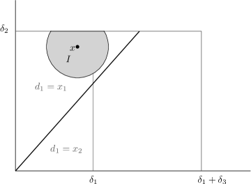
Figure 4. Domains of integration in Proposition 9.5.

Proposition 9.5.

Let $I=B(x,\frac{1}{2}d_{1}(x))\cap\widehat{D}$. Then

$$\left|P.V.\!\!\int_{I}\frac{\partial(G_{i}^{1}+G_{i}^{2})}{\partial x_{j}}\omega(y)~{}dy\right|\lesssim Mx_{i}^{-\alpha}(1+\delta_{j2}|\log d(x)|)$$

Proof.

Let $0<\delta<\frac{1}{2}d_{1}(x)$ so small such that $B(x,\delta)\subset\widehat{D}$. By Proposition 9.2,

(74) $$\begin{split}&\left|\int_{I\setminus B(x,\delta)}\sum_{k=1,2}\frac{\partial G_{i}^{k}}{\partial x_{j}}\omega(y)~{}dy\right|\lesssim\left|\int_{I\setminus B(x,\delta)}\sum_{k=1,2}\frac{\partial G_{i}^{k}}{\partial y_{j}}\omega(y)~{}dy\right|+\left|x_{i}^{-2}\int_{I\setminus B(x,\delta)}\mathcal{O}(|y-x|^{-1})\right|\end{split}$$

We distinguish the cases $i=j$ and $i\neq j$. First let $i=j$. Integration by parts gives

$$\begin{split}\text{\eqref{proofOfPropA3eq1}}&\lesssim\left|\int_{I\setminus B(x,\delta)}\sum_{k=1,2}G_{i}^{k}\frac{\partial\omega}{\partial y_{i}}(y)~{}dy\right|+\left|x_{i}^{-2}\int_{I\setminus B(x,\delta)}\mathcal{O}(|y-x|^{-1})\right|\\ &+\sum_{k=1,2}\left(\left|\int_{\partial I}G_{i}^{k}\omega(y)\nu_{i}~{}d\sigma\right|+\left|\int_{\partial B(x,\delta)}G_{i}^{k}\omega(y)\nu_{i}~{}d\sigma\right|\right).\end{split}$$

where $\nu=(\nu_{1},\nu_{2})$ is the unit outward pointing normal on $\partial I$. We first take care of the integral over $\partial I$. Observe that for $x\in D$, $\partial I$ is either a full circle is the union of a part of a circle and a flat part $\Sigma$. Hence

$$\int_{\partial I}|G_{i}^{k}\nu_{j}|~{}d\sigma \leq\int_{\Sigma}|G_{i}^{k}|\delta_{2i}~{}d\sigma+\int_{\partial B(0,\frac{1}{2}d_{1}(x))}|G_{i}^{k}|~{}d\sigma$$

For all sufficiently small $\varepsilon>0$,

$$\int_{\Sigma}|G_{i}^{k}|~{}d\sigma \leq\int_{\Sigma\cap\{|y_{1}-x_{1}|\leq\varepsilon\}}|G_{i}^{k}|~{}dy_{1}+\int_{\Sigma\cap\{|y_{1}-x_{1}|\geq\varepsilon\}}|G_{i}^{k}|~{}dy_{1}$$

$$\lesssim\int_{\Sigma\cap\{|y_{1}-x_{1}|\leq\varepsilon\}}\frac{x_{i}^{-1}}{|y-x|}~{}dy_{1}+\int_{\Sigma\cap\{|y_{1}-x_{1}|\geq\varepsilon\}}\frac{x_{i}^{-1}}{|y-x|}~{}dy_{1}$$

$$\lesssim x_{i}^{-1}\int_{x_{1}-\varepsilon}^{x_{1}+\varepsilon}\frac{1}{|x_{2}-\delta_{2}|}~{}dy_{1}+x_{i}^{-1}\int_{1>|x_{1}-y_{1}|>\varepsilon}\frac{1}{|y_{1}-x_{1}|}~{}dy_{1}$$

$$\lesssim\frac{x_{i}^{-1}\varepsilon}{|x_{2}-\delta_{2}|}+x_{i}^{-1}\int_{\varepsilon}^{1}\frac{1}{y_{1}}~{}dy_{1}$$

$$\lesssim\frac{x_{i}^{-1}\varepsilon}{|x_{2}-\delta_{2}|}+x_{i}^{-1}|\log\varepsilon|.$$

Here we used proposition 9.1 again. Choosing $\varepsilon=|x_{2}-\delta_{2}|=d(x)$ we get

$$\int_{\Sigma}|G_{i}^{k}|~{}d\sigma \lesssim x_{i}^{-1}(1+|\log d(x)|).$$

The other part is estimated by (using proposition 9.1 again)

$$\int_{\partial B(0,\frac{1}{2}d_{1}(x))}|G_{i}^{k}|~{}d\sigma \lesssim x_{i}^{-1}\int_{0}^{2\pi}|y-x|^{-1}d_{1}(x)~{}d\varphi\lesssim x_{i}^{-1}.$$

Therefore we get for the integral over $\partial I$, using (73) and (72):

$$\left|\int_{\partial I}G_{i}^{k}\omega(y)\nu_{i}~{}d\sigma\right| \lesssim\int_{\partial I}\left|G_{i}^{k}\nu_{i}\right|\left|\omega(y)\right|~{}d\sigma\lesssim M\int_{\partial I}\left|G_{i}^{k}\nu_{i}\right|y_{i}^{1-\alpha}~{}d\sigma$$

$$\lesssim Mx_{i}^{1-\alpha}\int_{\partial I}\left|G_{i}^{k}\nu_{i}\right|~{}d\sigma\lesssim Mx_{i}^{1-\alpha}x_{i}^{-1}(1+\delta_{i2}|\log d(x)|).$$

Similar estimates yield that the contribution from the integral over $\partial B(x,\delta)$ is $\lesssim Mx_{i}^{-\alpha}$, with universal constants independent of $\delta$. For

$$x_{i}^{-2}\int_{I\setminus B(x,\delta)}\mathcal{O}(|y-x|^{-1})|\omega(y)|dy$$

we obtain the upper bound $\lesssim Mx_{i}^{-\alpha}$ by the same methods.

For the remaining integral we use (72):

$$\left|\int_{I\setminus B(x,\delta)}G_{i}^{k}\frac{\partial\omega}{\partial y_{i}}(y)~{}dy\right| \lesssim Mx_{i}^{-\alpha}\int_{I\setminus B(x,\delta)}\left|G_{i}^{k}\right|~{}dy\lesssim Mx_{i}^{-\alpha}\int_{I\setminus B(x,\delta)}\left|y-x\right|^{-1}x_{i}^{-1}~{}dy$$

$$\lesssim Mx_{i}^{-\alpha}x_{i}^{-1}\int_{\delta}^{d_{1}(x)}\frac{1}{\rho}\rho~{}d\rho\lesssim Mx_{i}^{-\alpha}x_{i}^{-1}\int_{\delta}^{d_{1}(x)}\frac{1}{\rho}\rho~{}d\rho$$

$$\lesssim Mx_{i}^{-\alpha}x_{i}^{-1}d_{1}(x).$$

Since $d_{1}(x)\leq x_{i}$ we get:

$$\left|\int_{I\setminus B(x,\delta)}G_{i}^{k}\frac{\partial\omega}{\partial y_{j}}(y)~{}dy\right|\lesssim Mx_{i}^{-\alpha}.$$

This concludes the case $i=j$.

For the case $i\neq j$, we have to use the cancellation provided by Proposition 9.4 with $\gamma_{1}=2,\gamma_{2}=-1$.

$$\left|\int_{I\setminus B(x,\delta)}\frac{\partial(G_{i}^{1}+G_{i}^{2})}{\partial y_{j}}\omega(y)~{}\right|~{}dy \lesssim M\int_{I\setminus B(x,\delta)}\left|\frac{\partial(G_{i}^{1}+G_{i}^{2})}{\partial y_{j}}\right|y_{i}^{1-\alpha}~{}dy$$

$$\lesssim Mx_{i}^{1-\alpha}\int_{I\setminus B(x,\delta)}y_{i}^{-1}y_{j}^{-1}|y-x|^{-1}~{}dy$$

$$\lesssim Mx_{i}^{1-\alpha}x_{i}^{-1}x_{j}^{-1}\int_{\delta}^{d_{1}(x)}\frac{1}{\rho}\rho~{}d\rho$$

$$\lesssim Mx_{i}^{1-\alpha}x_{i}^{-1}x_{j}^{-1}d_{1}(x)\lesssim Mx_{i}^{-\alpha},$$

since $d_{1}(x)\lesssim x_{j}$. ∎

Lemma 9.6.

Let $\gamma\in(0,1)$ and $x_{1}\geq 0$. Then

$$y_{1}^{\gamma}\leq|y_{1}-x_{1}|^{\gamma}+x_{1}^{\gamma}\quad(y_{1}\geq 0).$$

Proof.

If $y_{1}\leq x_{1}$, the inequality is obvious. For $y_{1}>x_{1}$ we have $y_{1}\geq y_{1}-x_{1}>0$ and hence $\gamma y_{1}^{\gamma-1}\leq\gamma(y_{1}-x_{1})^{\gamma-1}$ so that

$$y_{1}^{\gamma}-x_{1}^{\gamma}\leq\gamma\int_{x_{1}}^{y_{1}}s^{\gamma-1}~{}ds\leq\gamma\int_{x_{1}}^{y_{1}}(s-x_{1})^{\gamma-1}~{}ds=(y_{1}-x_{1})^{\gamma}.$$

∎

Proposition 9.7.

Let $II=\widehat{D}\setminus I$ with $I$ as in proposition 9.5. Then

$$\left|\int_{II}\frac{\partial G_{i}^{k}}{\partial x_{j}}\omega(y)~{}dy\right|\lesssim Mx_{i}^{-\alpha}$$

Proof.

Here we have to distinguish two cases. Assume first $d_{1}(x)=x_{i}$. Then using proposition 9.1, (73) and Lemma 9.6 we have

$$\left|\int_{II}\frac{\partial G_{i}^{k}}{\partial x_{j}}\omega(y)~{}dy\right|\lesssim\int_{II}\left|\frac{\partial G_{i}^{k}}{\partial x_{j}}\right||\omega(y)|~{}dy$$

$$\lesssim M\int_{II}|y-x|^{-3}y_{i}^{1-\alpha}~{}dy\lesssim M\int_{II}|y-x|^{-3}(|y_{i}-x_{i}|^{1-\alpha}+x_{i}^{1-\alpha})$$

$$\lesssim M\int_{II}|y-x|^{-2-\alpha}~{}dy+Mx_{i}^{1-\alpha}\int_{II}|y-x|^{-3}$$

$$\lesssim M\int_{\frac{1}{2}d_{1}(x)}^{\infty}\frac{1}{\rho^{2+\alpha}}~{}\rho~{}d\rho+Mx_{i}^{1-\alpha}\int_{\frac{1}{2}d_{1}(x)}^{\infty}\frac{1}{\rho^{3}}~{}\rho~{}d\rho$$

$$\lesssim Md_{1}(x)^{-\alpha}+Mx_{i}^{1-\alpha}d_{1}(x)^{-1}\lesssim Mx_{i}^{-\alpha}+Mx_{i}^{1-\alpha}x_{i}^{-1}\lesssim Mx_{i}^{-\alpha}.$$

Now let $d_{1}(x)=x_{r}$, $r\neq i$. Without loss of generality, we write down only the case $i=1$ (so $d_{1}(x)=x_{2}$). From the explicit relations in Proposition 9.10 and the reflection inequalities we get

$$\left|\frac{\partial G_{1}^{k}}{\partial x_{i}}\right|\leq|y-x|^{-2}|y-\widetilde{x}|^{-1}$$

and hence again by (73) and Lemma 9.6,

$$\left|\int_{II}\frac{\partial G_{1}^{k}}{\partial x_{i}}\omega(y)~{}dy\right|\lesssim M\int_{II}\left|\frac{\partial G_{1}^{k}}{\partial x_{i}}\right|y_{2}^{1-\alpha}~{}dy$$

$$\lesssim M\int_{II}|y-x|^{-1-\alpha}|y-\widetilde{x}|^{-1}dy+Mx_{2}^{1-\alpha}\int_{II}|y-x|^{-2}|y-\widetilde{x}|^{-1}$$

We continue with the integral without the factor $x_{2}^{1-\alpha}$ in front; first we enlarge the integration domain by replacing $II$ with $\widehat{D}$, then we split the integration domain into a ball $B(0,2x_{1})$ and the rest.

$$\int_{\widehat{D}}|y-x|^{-1-\alpha}|y-\widetilde{x}|^{-1}dy\lesssim \int_{\widehat{D}\cap B(0,2x_{1})}|y-x|^{-1-\alpha}|y-\widetilde{x}|^{-1}dy$$

$$+\int_{\widehat{D}\setminus B(0,2x_{1})}|y-x|^{-1-\alpha}|y-\widetilde{x}|^{-1}dy$$

$$\lesssim ~{}x_{1}^{-1}\int_{\widehat{D}\cap B(x,10x_{1})}|y-x|^{-1-\alpha}dy+\int_{B(0,10)\setminus B(0,2x_{1})}|y|^{-2-\alpha}dy$$

$$\lesssim ~{}x_{1}x_{1}^{1-\alpha}+x_{1}^{-\alpha}\lesssim x_{1}^{-\alpha}.$$

Here, we used that $x_{2}\leq x_{1}$ (since $d_{1}(x)=x_{2}$), so that $|y|\lesssim|y-x|,|y|\lesssim|y-\widetilde{x}|$ in the second integral. Continuing with $x_{2}^{1-\alpha}\int_{II}|y-x|^{-2}|y-\widetilde{x}|^{-1}$, we get

$$x_{2}^{1-\alpha}\int_{II}|y-x|^{-2}|y-\widetilde{x}|^{-1}dy\lesssim x_{2}^{1-\alpha}x_{1}^{-\alpha}\int_{II}|y-x|^{-3+\alpha}dy$$

$$\lesssim x_{2}^{1-\alpha}x_{1}^{-\alpha}x_{2}^{-1+\alpha}\alpha x_{1}^{-\alpha}$$

using $|y-\widetilde{x}|\geq x_{1}^{\alpha}|y-\widetilde{x}|^{1-\alpha}\geq x_{1}^{\alpha}|y-x|^{1-\alpha}$. ∎

Proposition 9.8.

For $i\neq j$,

$$\left|\int_{{[0,1]^{2}}\setminus\widehat{D}}\left[\frac{\partial G_{i}^{1}}{\partial x_{j}}+\frac{\partial G_{i}^{2}}{\partial x_{j}}\right]\omega(y)~{}dy\right|\leq~{}~{}C(\gamma_{1},\gamma_{2})x_{i}^{-(\gamma_{1}+\gamma_{2})}x_{j}^{\gamma_{2}}d(x)^{-1+\gamma_{1}}$$

where $\gamma_{1}\in(0,1),\gamma_{2}\in[0,1),\gamma_{1}+\gamma_{2}<1$. Also,

$$\left|\int_{{[0,1]^{2}}\setminus\widehat{D}}\left[\frac{\partial G_{i}^{i}}{\partial x_{1}}+\frac{\partial G_{i}^{2}}{\partial x_{i}}\right]\omega(y)~{}dy\right|\leq~{}~{}C(\gamma_{1})x_{i}^{-\gamma_{1}}d(x)^{-1+\gamma_{1}}$$

Proof.

As a preparation, we note that for $x\in D$, $0<\gamma_{1}<1$,

(75) $$\int_{{[0,1]^{2}}\setminus\widehat{D}}|y-x|^{-3+\gamma_{1}}\lesssim d(x)^{-1+\gamma_{1}}.$$

This follows from

$$\int_{{[0,1]^{2}}\setminus\widehat{D}}|y-x|^{-3+\gamma_{1}} \leq\int_{{[0,1]^{2}}\setminus B(x,d(x))}|y-x|^{-3+\gamma_{1}}$$

$$\leq\int_{B(x,10)\setminus B(x,d(x))}|y-x|^{-3+\gamma_{1}},$$

since ${[0,1]^{2}}\setminus\widehat{D}$ is contained in ${[0,1]^{2}}\setminus B(x,d(x))$ because of $\delta_{2}<\delta_{3}$ and $\delta_{1}<\delta_{2}$.

From Proposition 9.4 we get in case $i\neq j$

$$\left|\int_{{[0,1]^{2}}\setminus\widehat{D}}\left[\frac{\partial G_{i}^{1}}{\partial x_{1}}+\frac{\partial G_{i}^{2}}{\partial x_{j}}\right]\omega(y)~{}dy\right| \leq x_{i}^{-(\gamma_{1}+\gamma_{2})}x_{j}^{\gamma_{2}}\int_{{[0,1]^{2}}\setminus\widehat{D}}|y-x|^{-3+\gamma_{1}}$$

$$\leq x_{i}^{-(\gamma_{1}+\gamma_{2})}x_{j}^{\gamma_{2}}d(x)^{-1+\gamma_{1}},$$

according to (75).

For the second inequality of the Proposition, we note that

$$\left|\frac{\partial G_{i}^{k}}{\partial x_{i}}\right| \lesssim x_{i}^{-\gamma_{1}}|y-x|^{-3+\gamma_{1}},$$

and use (75). ∎

Proposition 9.9.

For $x\in D$,

$$\left|P.V.\!\!\int_{{[0,1]^{2}}}\left[\frac{\partial G_{i}^{1}}{\partial x_{j}}+\frac{\partial G_{i}^{2}}{\partial x_{j}}\right]\omega(y)~{}dy\right| \leq Mx_{i}^{-\alpha}(1+\delta_{j2}|\log d(x)|)$$

$$\,\,+C(\gamma_{1},\gamma_{2})x_{i}^{-(\gamma_{1}+\gamma_{2})}x_{j}^{\gamma_{2}}d(x)^{-1+\gamma_{1}}\quad(i\neq j)$$

$$\left|P.V.\!\!\int_{{[0,1]^{2}}}\left[\frac{\partial G_{i}^{1}}{\partial x_{i}}+\frac{\partial G_{i}^{2}}{\partial x_{i}}\right]\omega(y)~{}dy\right| \leq Mx_{i}^{-\alpha}(1+\delta_{i2}|\log d(x)|)+C(\gamma_{1})x_{i}^{-\gamma_{1}}d(x)^{-1+\gamma_{1}}$$

with $\gamma,\gamma_{1}\in(0,1),\gamma_{2}\in[0,1),\gamma_{1}+\gamma_{2}<1$.

Proof.

We split the integral into a principal value integral over $\widehat{D}$ and a convergent integral over ${[0,1]^{2}}\setminus\widehat{D}$. The integral over $\widehat{D}$ is further split in to integrals over the domains $I=B(x,\frac{1}{2}d_{1}(x))$ and $II=\widehat{D}\setminus I$, which are estimated by Propositions 9.5 and 9.7. The part over ${[0,1]^{2}}\setminus\widehat{D}$ is estimated by Proposition 9.8. ∎

9.2. Appendix B

Derivation of $Q_{i}$ and $G_{i}^{j}$.

In all integrals over infinite domains it is understood that $\omega$ is extended periodically and the integrals are understood as limits in the mean. We derive only $Q_{1}$ and the formulas for $G_{1}^{1},~{}G_{1}^{2}$. $Q_{2},~{}G_{2}^{1}$ and $G_{2}^{2}$ are analogous. The first component of the velocity field is

$$u_{1}(x,t) =\frac{1}{2\pi}\int_{\mathbb{R}^{2}}\frac{-(y_{2}-x_{2})}{|y-x|^{2}}\omega(y,t)~{}dy$$

$$=\frac{1}{2\pi}\left\{\int_{(0,\infty)^{2}}+\int_{(-\infty,0)\times(0,\infty)}+\int_{(0,\infty)\times(-\infty,0)}+\int_{(-\infty,0)^{2}}\right\}\frac{-(y_{2}-x_{2})}{|y-x|^{2}}\omega(y,t)~{}dy.$$

Recall $\widetilde{x}=(-x_{1},x_{2}),~{}\overline{x}=(x_{1},-x_{2})$. Using the double-odd symmetry of $\omega$ we can write

$$\int_{(-\infty,0)\times(0,\infty)}\frac{-(y_{2}-x_{2})}{|y-x|^{2}}\omega(y,t)~{}dy =\int_{(0,\infty)^{2}}\frac{y_{2}-x_{2}}{|y-\widetilde{x}|^{2}}\omega(y,t)~{}dy$$

$$\int_{(0,\infty)\times(-\infty,0)}\frac{-(y_{2}-x_{2})}{|y-x|^{2}}\omega(y,t)~{}dy =\int_{(0,\infty)^{2}}\frac{-(y_{2}+x_{2})}{|y-\overline{x}|^{2}}\omega(y,t)~{}dy$$

$$\int_{(-\infty,0)^{2}}\frac{-(y_{2}-x_{2})}{|y-x|^{2}}\omega(y,t)~{}dy =\int_{(0,\infty)^{2}}\frac{y_{2}+x_{2}}{|y+x|^{2}}\omega(y,t)~{}dy.$$

Next we group the integrals in the following way

$$\int_{(0,\infty)^{2}}\frac{-(y_{2}-x_{2})}{|y-x|^{2}}\omega(y,t)~{}dy+\int_{(0,\infty)^{2}}\frac{y_{2}-x_{2}}{|y-\widetilde{x}|^{2}}\omega(y,t)~{}dy$$

$$= -4x_{1}\int_{(0,\infty)^{2}}\underbrace{\frac{y_{1}(y_{2}-x_{2})}{|y-x|^{2}|y-\widetilde{x}|^{2}}}_{G_{1}^{1}(x,y)}\omega(y,t)~{}dy$$

$$\int_{(0,\infty)^{2}}\frac{-(y_{2}+x_{2})}{|y-\overline{x}|^{2}}\omega(y,t)~{}dy+\int_{(0,\infty)^{2}}\frac{y_{2}+x_{2}}{|y+x|^{2}}\omega(y,t)~{}dy$$

$$= -4x_{1}\int_{(0,\infty)^{2}}\underbrace{\frac{y_{1}(y_{2}+x_{2})}{|y+x|^{2}|y-\overline{x}|^{2}}}_{G_{1}^{2}(x,y)}\omega(y,t)~{}dy.$$

Together we obtain

$$u_{1}(x,y)= -x_{1}\frac{2}{\pi}\int_{[0,1]^{2}}[G_{1}^{1}(x,y)+G_{1}^{2}(x,y)]\omega(y,t)~{}dy$$

$$-x_{1}\frac{2}{\pi}\int_{\mathbb{R}_{+}^{2}\setminus[0,1]^{2}}[G_{1}^{1}(x,y)+G_{1}^{2}(x,y)]\omega(y,t)~{}dy$$

$$= -x_{1}\left(\frac{2}{\pi}\int_{[0,1]^{2}}[G_{1}^{1}(x,y)+G_{1}^{2}(x,y)]\omega(y,t)~{}dy+Q_{1}^{r}(x,t)\right)=-x_{1}Q_{1}(x,t).$$

Proposition 9.10.

The following relations hold:

$$\frac{\partial G_{1}^{1}}{\partial x_{1}} =-\frac{2y_{1}(y_{1}+x_{1})(y_{2}-x_{2})}{|y-x|^{2}|y-\widetilde{x}|^{4}}+\frac{2y_{1}(y_{1}-x_{1})(y_{2}-x_{2})}{|y-x|^{4}|y-\widetilde{x}|^{2}}$$

$$\frac{\partial G_{1}^{1}}{\partial x_{2}} =\frac{2y_{1}(y_{2}-x_{2})^{2}}{|y-x|^{2}|y-\widetilde{x}|^{4}}+\frac{2y_{1}(y_{2}-x_{2})^{2}}{|y-x|^{4}|y-\widetilde{x}|^{2}}-\frac{y_{1}}{|y-x|^{2}|y-\widetilde{x}|^{2}}$$

$$\frac{\partial G_{1}^{1}}{\partial y_{1}} =-\frac{2y_{1}(y_{1}+x_{1})(y_{2}-x_{2})}{|y-x|^{2}|y-\widetilde{x}|^{4}}-\frac{2y_{1}(y_{1}-x_{1})(y_{2}-x_{2})}{|y-x|^{4}|y-\widetilde{x}|^{2}}+\frac{y_{2}-x_{2}}{|y-x|^{2}|y-\widetilde{x}|^{2}}$$

$$\frac{\partial G_{1}^{1}}{\partial y_{2}} =-\frac{2y_{1}(y_{2}-x_{2})^{2}}{|y-x|^{2}|y-\widetilde{x}|^{4}}-\frac{2y_{1}(y_{2}-x_{2})^{2}}{|y-x|^{4}|y-\widetilde{x}|^{2}}+\frac{y_{1}}{|y-x|^{2}|y-\widetilde{x}|^{2}}$$

$$\frac{\partial G_{1}^{2}}{\partial x_{1}} =-\frac{2y_{1}(y_{1}+x_{1})(y_{2}+x_{2})}{|y+x|^{4}|y-\overline{x}|^{2}}+\frac{2y_{1}(y_{1}-x_{1})(y_{2}+x_{2})}{|y+x|^{2}|y-\overline{x}|^{4}}$$

$$\frac{\partial G_{1}^{2}}{\partial x_{2}} =-\frac{2y_{1}(y_{2}+x_{2})^{2}}{|y+x|^{4}|y-\overline{x}|^{2}}-\frac{2y_{1}(y_{2}+x_{2})^{2}}{|y+x|^{2}|y-\overline{x}|^{4}}+\frac{y_{1}}{|y+x|^{2}|y-\overline{x}|^{2}}$$

$$\frac{\partial G_{1}^{2}}{\partial y_{1}} =-\frac{2y_{1}(y_{1}+x_{1})(y_{2}+x_{2})}{|y+x|^{4}|y-\overline{x}|^{2}}-\frac{2y_{1}(y_{1}-x_{1})(y_{2}+x_{2})}{|y+x|^{2}|y-\overline{x}|^{4}}+\frac{y_{2}+x_{2}}{|y+x|^{2}|y-\overline{x}|^{2}}$$

$$\frac{\partial G_{1}^{2}}{\partial y_{2}} =-\frac{2y_{1}(y_{2}+x_{2})^{2}}{|y+x|^{4}|y-\overline{x}|^{2}}-\frac{2y_{1}(y_{2}+x_{2})^{2}}{|y+x|^{2}|y-\overline{x}|^{4}}+\frac{y_{1}}{|y+x|^{2}|y-\overline{x}|^{2}}$$

$$\frac{\partial G_{2}^{1}}{\partial x_{1}} =-\frac{2y_{2}(y_{1}+x_{1})^{2}}{|y+x|^{4}|y-\widetilde{x}|^{2}}-\frac{2y_{2}(y_{1}+x_{1})^{2}}{|y+x|^{2}|y-\widetilde{x}|^{4}}+\frac{y_{2}}{|y+x|^{2}|y-\widetilde{x}|^{2}}$$

$$\frac{\partial G_{2}^{1}}{\partial x_{2}} =-\frac{2y_{2}(y_{1}+x_{1})(y_{2}+x_{2})}{|y+x|^{4}|y-\widetilde{x}|^{2}}+\frac{2y_{2}(y_{1}+x_{1})(y_{2}-x_{2})}{|y+x|^{2}|y-\widetilde{x}|^{4}}$$

$$\frac{\partial G_{2}^{1}}{\partial y_{1}} =-\frac{2y_{2}(y_{1}+x_{1})^{2}}{|y+x|^{4}|y-\widetilde{x}|^{2}}-\frac{2y_{2}(y_{1}+x_{1})^{2}}{|y+x|^{2}|y-\widetilde{x}|^{4}}+\frac{y_{2}}{|y+x|^{2}|y-\widetilde{x}|^{2}}$$

$$\frac{\partial G_{2}^{1}}{\partial y_{2}} =-\frac{2y_{2}(y_{1}+x_{1})(y_{2}+x_{2})}{|y+x|^{4}|y-\widetilde{x}|^{2}}-\frac{2y_{2}(y_{1}+x_{1})(y_{2}-x_{2})}{|y+x|^{2}|y-\widetilde{x}|^{4}}+\frac{y_{1}+x_{1}}{|y+x|^{2}|y-\widetilde{x}|^{2}}$$

$$\frac{\partial G_{2}^{2}}{\partial x_{1}} =\frac{2y_{2}(y_{1}-x_{1})^{2}}{|y-x|^{2}|y-\overline{x}|^{4}}+\frac{2y_{2}(y_{1}-x_{1})^{2}}{|y-x|^{4}|y-\overline{x}|^{2}}-\frac{y_{2}}{|y-x|^{2}|y-\overline{x}|^{2}},$$

$$\frac{\partial G_{2}^{2}}{\partial x_{2}} =-\frac{2y_{2}(y_{1}-x_{1})(y_{2}+x_{2})}{|y-x|^{2}|y-\overline{x}|^{4}}+\frac{2y_{2}(y_{1}-x_{1})(y_{2}-x_{2})}{|y-x|^{4}|y-\overline{x}|^{2}},$$

$$\frac{\partial G_{2}^{2}}{\partial y_{1}} =-\frac{2y_{2}(y_{1}-x_{1})^{2}}{|y-x|^{2}|y-\overline{x}|^{4}}-\frac{2y_{2}(y_{1}-x_{1})^{2}}{|y-x|^{4}|y-\overline{x}|^{2}}+\frac{y_{2}}{|y-x|^{2}|y-\overline{x}|^{2}},$$

$$\frac{\partial G_{2}^{2}}{\partial y_{2}} =-\frac{2y_{2}(y_{1}-x_{1})(y_{2}+x_{2})}{|y-x|^{2}|y-\overline{x}|^{4}}-\frac{2y_{2}(y_{1}-x_{1})(y_{2}-x_{2})}{|y-x|^{4}|y-\overline{x}|^{2}}+\frac{y_{1}-x_{1}}{|y-x|^{2}|y-\overline{x}|^{2}}.$$

References

- [1] H. Bahouri, J.-Y. Chemin, Equations de transport relatives a des champs de vecteurs non-Lipschitziens et mechanique de fluides, (French) Arch. Rational Mech. Anal. 127, 2, 159-181 (1994).
- [2] D. Córdoba: Nonexistence of Simple Hyperbolic Blow-Up for the Quasi-Geostrophic Equation, Ann. Math., Second Series, Vol. 148, No. 3 (1998), 1135-1152
- [3] D. Córdoba, C. Fefferman: Growth of Solutions for QG and 2D Euler Equations, Journal of the American Mathematical Society, 15, 3, p. 665-670 (2002).
- [4] S. Denissov: Infinite superlinear growth of the gradient for the two-dimensional Euler equation, Discrete Contin. Dyn. Syst. A 23 (2009), 755-764.
- [5] S. Denissov: Double-exponential growth of the vorticity gradient for the two-dimensional Euler equation, Proceedings of the AMS, Vol. 143, N3, 2015, 1199-1210.
- [6] S. Denissov: The sharp corner formation in 2D Euler dynamics of patches: infinite double-exponential rate of merging, Arch. Rational Mech. Anal., Vol. 215, N2, 2015, 675-705.
- [7] N. H. Katz and A. Tapay, A model for studying double exponential growth in the two-dimensional Euler equations, preprint arXiv:1403.6867.
- [8] A. Kiselev and V. Šverák, Small scale creation for solutions of the incompressible two dimensional Euler equation, Annals of Math. 180 (2014), 1205–1220.
- [9] W. Walter, Differential and Integral Inequalities, Springer 1970.
- [10] D. Wilett, A Linear Generalization of Gronwall’s inequality, Trans. Am. Math. Soc, 16, 774-778 (1965).
- [11] A. Zlatoš, Exponential growth of the vorticity gradient for the Euler equation on the torus, Adv. Math. 268 (2015), 396-403.