Does the “uptick rule” stabilize the stock market? Insights from Adaptive Rational Equilibrium Dynamics

Abstract

This paper investigates the effects of the “uptick rule” (a short selling regulation formally known as rule 10a- 1) by means of a simple stock market model, based on the ARED (adaptive rational equilibrium dynamics) modeling framework, where heterogeneous and adaptive beliefs on the future prices of a risky asset were first shown to be responsible for endogenous price fluctuations.

The dynamics of stock prices generated by the model, with and without the uptick-rule restriction, are analyzed by pairing the classical fundamental prediction with beliefs based on both linear and nonlinear technical analyses. The comparison shows a reduction of downward price movements of undervalued shares when the short selling restriction is imposed. This gives evidence that the uptick rule meets its intended objective. However, the effects of the short selling regulation fade when the intensity of choice to switch trading strategies is high. The analysis suggests possible side effects of the regulation on price dynamics.

Keywords: Asset pricing model, Heterogeneous beliefs, Endogenous price fluctuations, Piecewise-smooth dynamical systems, Chaos, Uptick-rule.

JEL codes: C62, G12, G18

1 Introduction

Short selling is the practice of selling financial instruments that have been borrowed, typically from a broker-dealer or an institutional investor, with the intent to buy the same class of financial instruments in a future period and return them back at the maturity of the loan.

By short selling, investors open a so-called “short position”, that is technically equivalent to holding a negative amount of shares of the traded asset, with the expectation that the asset will recede in value in the next period. At the closing time specified in the short selling contract, the debt is compounded with interest which occurred during the period of the financial operation, for this reason short sellers prefer to close the short position and reopen a new one with the same features, rather than extending the position over the closing time (see, e.g., (Hull, 2011)).

A short position is the counterpart of the (more conventional) “long position”, i.e. buying a security such as a stock, commodity, or currency, with the expectation that the asset will rise in value.

Short selling is considered the father of the modern derivatives and, as such, it has a double function: it can be used as an insurance device, by hedging the risk of long positions in related stocks thus allowing risky financial operations, or for speculative purposes, to profit from an expected downward price movement. Moreover, financial speculators can sell short stocks in an effort to drive down the related price by creating an imbalance of sell-side interest, the so called “bear raid” action. This feedback may lead to the market collapse, and has indeed been observed during the financial crises of 1937 and 2007, see, e.g., (Misra et al., 2012).

Many national authorities have developed different kinds of short selling restrictions to avoid the negative effect of this financial practice. Most of the regulations are based on “price tests”, i.e., short selling is allowed or restricted depending on some tests based on recent price movements. The best known and most widely applied of such regulations is the so-called “uptick rule”, or rule 10a-1, imposed in 1938 by the U.S. Securities and Exchange Commission (hereafter SEC) to protect investors and was in force until 2007. This rule regulated short selling into all U.S. stock markets and in the Toronto Stock Exchange. Other financial markets, like the London Stock Exchange and the Tokyo Stock Exchange, have different or no short selling restrictions (for a summary of short sale regulations in approximately 50 different countries see (Bris et al., 2007)).

The uptick rule originally stated that short sales are allowed only on an uptick, i.e., at a price higher than the last reported transaction price. The rule was later relaxed to allow short sales to take place on a zero-plus-tick as well, i.e., at a price that is equal to the last sale price but only if the most recent price movement has been positive. Conversely, short sales are not permitted on minus- or zero-minus-ticks, subject to narrow exceptions.

In adopting the uptick rule, the SEC sought to achieve three objectives:

• allowing relatively unrestricted short selling in an advancing market;

• preventing short selling at successively lower prices, thus eliminating short selling as a tool for driving the market down; and

• preventing short sellers from accelerating a declining market by exhausting all remaining bids at one price level, causing successively lower prices to be established by long sellers.

The last two objectives have been partially confirmed by the empirical analysis (see, e.g., (Alexander and Peterson, 1999) and reference therein). Instead, the regulation does not seem to be effective in producing the first desired effect. The observed number of executed short sales is indeed lower under uptick rule than in the unconstrained case, during phases with an upward market trend, see again (Alexander and Peterson, 1999). This is due to the asynchrony between placement and execution of a short-sell order, since the rising of the price in between these two operations can make the trade not feasible under the uptick rule.

Moreover, empirical evidence provides uniform support of the idea that short selling restrictions often cause share prices to rise. From a theoretical point of view, there is no clear argument for explaining this mispricing effect of the uptick rule. According to (Miller, 1977) this is due to a reduction in stock supply owing to the short sale restriction. More generally, theoretical models with heterogeneous agents and differences in trading strategies support the idea that share values become overvalued under short selling restrictions due to the fact that “pessimistic” and “bear” traders (expecting negative price movements) are ruled out of the market (see, e.g., (Harrison and Kreps, 1978)). In contrast, theoretical models based on the assumption that all agents have rational expectations suggest that short selling restrictions do not change on the average the stock prices (see, e.g., (Diamond and Verrecchia, 1987)).

However, given the complexity of the phenomena, and the impossibility of isolating the effects of a regulation from other concomitant changes in the economic scenario, the effectiveness of the uptick rule in meeting the three above objectives, and its possible side effects on shares’ prices, are still far from being completely clarified.

Guided by the aim to provide further insight on the argument, this paper studies the effects on share prices in an artificial market of a short selling restriction based on a tick test similar to the one imposed by the uptick rule in real financial markets. Using an artificial asset pricing model makes it easier in assessing the effects of the uptick rule in isolation from other exogenous shocks, though artificial modeling necessarily trades realism for mathematical tractability.

We consider an asset pricing model of adaptive rational equilibrium dynamics (A.R.E.D.), where heterogeneous beliefs on the future prices of a risky asset, together with traders’ adaptability based on past performances, have shown to endogenously sustain price fluctuations. Asset pricing models of A.R.E.D. (hereafter referred to simply as ARED asset pricing models) are discrete-time dynamical systems based on the empirical evidence that investors with different trading strategies coexist in the financial market (see, e.g., (Taylor and Allen, 1992)). These simple models provide a theoretical justification for many “stylized facts” observed in the real financial time series, such as, financial bubbles and volatility clustering (see (Gaunersdorfer, 2001), and (Gaunersdorfer et al., 2008)). Stochastic models based on the same assumptions are even used to study exchange rate volatility and the implication of some specific financial policies (see, e.g., (Westerhoff, 2001)).

We extend, in particular, the deterministic model introduced in (Brock and Hommes, 1998), where, in the simplest case, agents choose between two predictors of future prices of a risky asset, i.e. a fundamental predictor and a non-fundamental predictor. Agents that adopt the fundamental predictor are called fundametalists, while agents that adopt the non-fundamental predictor are called noise traders or non-fundamental traders. Fundamentalists believe that the price of a financial asset is determined by its fundamental value (as given by the present discounted value of the stream of future dividends, see (Hommes, 2001)) and any deviation from this value is only temporary. Non-fundamental traders, sometimes called chartists or technical analysts, believe that the future price of a risky asset is not completely determined by fundamentals and it can be predicted by simple technical trading rules (see, e.g., (Elder, 1993), (Murphy, 1999), and (Nelly, 1997)).

In the model, agents revise their "beliefs", prediction to be adopted, according to an evolutionary mechanism based on the past realized profits. As a result, the fundamental value is a fixed point of the price dynamics, as, once there, both fundamentalists and non-fundamental traders predict the fundamental price. As long as the sensitivity of traders in switching to the best performing predictor is relatively low, the fundamental equilibrium is stable, but the fundamental stability is typically lost at higher intensities of the traders’ choice across the predictors, making room for financial bubbles.

It is worth to remember that (Brock and Hommes, 1998) investigated the peculiar case of zero supply of outside shares. Under this assumption each bought share is sold short. We therefore consider a positive supply of outside share, that is essential to ensure financial transactions when short selling is forbidden. Moreover, we pair the fundamental predictor with first a technical linear predictor and then with a technical nonlinear predictor and compare the results obtained with and without the uptick rule.

As linear predictor, we consider the chartist predictor introduced in (Brock and Hommes, 1998). This facilitates the comparison of our results with those in (Brock and Hommes, 1998) and related papers. As nonlinear predictor, we introduce a new predictor, "Smoothed Price Rate Of Change" or S-ROC predictor, that extrapolates future prices by applying the rate of change averaged on past prices with a confidence mechanism smoothing out extreme unrealistic rates (for an overview of this class of predictors, see (Elder, 1993)).

For what concerns the implementation of the regulation, we implement the uptick rule as it was in its original formulation, i.e., short selling is allowed only on an uptick. Note, however, that in an artificial asset pricing model a zero-tick is possible only at equilibrium, so that allowing or forbidding short sales on zero-plus-ticks makes basically no change in the observed price dynamics. In fact, with a positive supply of shares, traders take long positions at the fundamental equilibrium, so only the non-fundamental equilibria at which one type of trader is prohibited to go short are affected by the rule behavior on zero-plus-ticks (moreover, such equilibria are irrelevant to study the global price dynamics, as will be explained in Section 2.3).

From the mathematical point of view, the uptick rule makes the asset pricing model a piecewise-smooth dynamical system, namely a system in which different mathematical rules can be applied to determine the next price, and the rule to be applied depends on the current state of the system, that is, on the fact that trader types are interested in going short and whether short selling is allowed or not. Non-smooth dynamical systems are certainly more problematic to analyze, both analytically and numerically (though non-smooth dynamics is a very active topic in current research, see (di Bernardo et al., 2008), and (Colombo et al., 2012), and references therein) so we will limit the analytical treatment to stationary solutions.

Piecewise-smooth dynamical systems have already been used as models in finance. (Tramontana et al., 2011) proposed a one-dimensional piecewise-linear asset pricing model, where traders adopt different buying and selling strategies in response to different market movements. Other examples can be found in (Tramontana et al., 2010a), (Tramontana et al., 2010b), and (Tramontana and Westerhoff, 2013). Two ARED piecewise-smooth systems modeling short selling restrictions have been also proposed. Modifying the model in (Brock and Hommes, 1998), (Anufriev and Tuinstra, 2009) restricted short selling by allowing limited short positions at each trading period, whereas (Dercole and Cecchetto, 2010) investigated the complete ban on short selling. Thus both contributions implement short selling restrictions that are not based on price tests.

The results of our theoretical analyses are in line with the empirical evidence. The sale price that is established in our model when one trader type is prohibited from going short is indeed systematically higher than the unconstrained price. Thus, constrained downward movements below the fundamental value are less pronounced, whereas constrained upward movements above the fundamental value can be larger. We provide a more complete explanation for this effect, suggesting that it is due to the combination of two mechanisms: on one side, the short selling restriction reduces the possibility for pessimistic or bear traders to bet on downward movements below the fundamental value, avoiding excessive underpricing, but at the same time, when prices are above the fundamental value, the restriction reduces the possibility for fundamentalists to drive down the prices back to the fundamental value by opening short positions. This is in agreement with the last two goals established by the SEC (see above). The first stated objective of the uptick is always realized in our model, since the market clearing is assumed to be synchronous among all traders.

When non-fundamental traders adopt the S-ROC predictor, we observe that the overpricing due to the uptick rule disappears due to the smoothness of the predictor that makes non-fundamental traders not confident with extreme price deviations from the fundamental value. Indeed, the expectations of large price deviations produced by the uptick rule force the non-fundamental trader to believe in the fundamental value with the effect of reducing, instead of increasing, the price deviations. The stabilizing effect however vanishes when traders become highly sensitive in switching to the strategy with best recent performance.

The paper is organized as follows. Section 2.1 briefly reviews the unconstrained asset pricing model, summarizing from (Brock and Hommes, 1998) and setting the notation and most of the modeling equations that will be used in next Sections. Section 2.2 is also preliminary and recaps the concept of fundamental equilibrium, including its stability analysis and some new results. Section 2.3 formulates the piecewise-smooth model constrained by the uptick rule, and discusses the existence and stability of fundamental and non-fundamental equilibria. So far, no explicit price predictors is introduced, whereas Section 2.4 presents the price predictors for which the unconstrained and constrained models will be studied and compared in Sections 3 and 4. Section 3 presents the analytical results concerning the existence and stability of fixed points. Some of the results concerning the unconstrained model are new and interesting per se. Section 4 presents a series of numerical tests, confirming the analytical results and investigating non-stationary (periodic, quasi-periodic, and chaotic) regimes. In Section 4.3 we discuss in detail our economic findings. Section 5 concludes and lists a series of related interesting topics for further research. All the analytical results presented in Sections 2 and 3 are proved in Appendix 6.

2 The ARED asset pricing model with and without the uptick rule

We consider the asset pricing model with heterogeneous beliefs and adaptive traders introduced by (Brock and Hommes, 1998). While in the original model a zero supply of outside shares was considered, making short selling essential to ensure the exchanges, we consider the case of positive supply, so that short selling will no longer be necessary and a constraint on it can be imposed. In this generalized version of the original model, we introduce a negative demand constraint according to the uptick rule, in order to study the effects of this regulation on price fluctuations.

2.1 The unconstrained ARED asset pricing model

Consider a financial market where traders invest either in a single risky asset, supplied in $S$ shares of (ex-dividend) price $p_{t}$ at period $t$, or in a risk free asset perfectly elastically supplied at gross return $R$ (where $R=1+r$, with $r\in(0,1)$). The risky asset pays random dividend $\tilde{y}_{t}$ in period $t$, where the divided process $\tilde{y}_{t}$ is IID (Identically Independently Distributed) with $E_{t}\left[\tilde{y}_{t+1}\right]=\bar{y}$ constant. Thus, denoting by $W_{h,t}$ the economic wealth of a generic trader of type $h$ at the beginning of period $t$, and by $z_{h,t}$ the number of shares held by the trader in period $t$, we have the following wealth equation (or individual intertemporal budget constraint):

$$\tilde{W}_{h,t+1}=R(W_{h,t}-p_{t}z_{h,t})+\tilde{p}_{t+1}z_{h,t}+\tilde{y}_{t+1}z_{h,t}=RW_{h,t}+(\tilde{p}_{t+1}+\tilde{y}_{t+1}-R\hskip 0.56905ptp_{t})z_{h,t},$$ (1)

where tilde denotes random variables, $W_{h,t}-p_{t}z_{h,t}$ is the amount of money invested in the risk free asset in period $t$ and $\tilde{R}_{t+1}=\tilde{p}_{t+1}+\tilde{y}_{t+1}-R\hskip 0.56905ptp_{t}$ is the excess return per share realized at the end of the period.

Let $E_{h,t},V_{h,t}$ denote the "beliefs" of investor of type $h$ about the conditional expectation and conditional variance of wealth. They are assumed to be functions of past prices and dividends. We assume that each investor type is a myopic mean variance maximizer, so for type $h$ the demand for shares $z_{h,t}$ solves

$$\max_{z_{h,t}}\left\{E_{h,t}\left(\tilde{W}_{t+1}\right)-\frac{a}{2}V_{h,t}\left(\tilde{W}_{t+1}\right)\right\}$$

i.e.,

$$z_{h,t}\left(p_{t}\right)=\displaystyle\frac{\displaystyle E_{h,t}[\tilde{R}_{t+1}]}{\displaystyle aV_{h,t}[\tilde{R}_{t+1}]}=\displaystyle\frac{\displaystyle E_{h,t}[\tilde{p}_{t+1}+\tilde{y}_{t+1}]-R\hskip 0.56905ptp_{t}}{\displaystyle aV_{h,t}[\tilde{R}_{t+1}]},$$

where $a$ is the risk aversion coefficient and $p_{t}$ is to be determined by the market clearing between all demands and the supply $S$ of shares. For simplicity (as done in (Brock and Hommes, 1998), see (Gaunersdorfer, 2000), for an extension), we assume that traders have common and constant beliefs about the variance, i.e. $V_{h,t}\left[\tilde{R}_{t+1}\right]=\sigma^{2}$, $\forall h$, and common and correct beliefs about the dividend, i.e. $E_{h,t}\left[\tilde{y}_{t+1}\right]=E_{t}\left[\tilde{y}_{t+1}\right]=\bar{y}$, $\forall h$. Moreover, the number $N$ of traders and $S$ of supplied shares in each period (not considering the extra supply of shares due to short sales) are kept constant. Let $H$ be the number of available "beliefs" or price predictors $E_{h,t}[\tilde{p}_{t+1}+\tilde{y}_{t+1}]$, $h=1,\ldots,H$, each obtained at a cost $C_{h}$, and denote by $n_{h,t}$ the fraction of traders adopting predictor $h$ in period $t$, the market clearing imposes

$$N\sum_{h=1}^{H}n_{h,t}z_{h,t}(p_{t})=S,\quad z_{h,t}(p_{t})=\frac{\displaystyle E_{h,t}[\tilde{p}_{t+1}+\tilde{y}_{t+1}]-R\hskip 0.56905ptp_{t}}{\displaystyle a\hskip 0.56905pt\sigma^{2}},$$ (2)

which is solved for $p_{t}$, thus obtaining

$$p_{t}=\displaystyle\frac{\displaystyle 1}{\displaystyle R}\left(\sum_{h=1}^{H}n_{h,t}E_{h,t}[\tilde{p}_{t+1}+\tilde{y}_{t+1}]-a\hskip 0.56905pt\sigma^{2}\displaystyle\frac{\displaystyle S}{\displaystyle N}\right),$$ (3)

Let us substitute the expression of $p_{t}$ in $z_{h,t}\left(p_{t}\right)$, $\forall h\in H$, to obtain the actual demands

$$z_{h,t}=\displaystyle\frac{\displaystyle 1}{\displaystyle a\hskip 0.56905pt\sigma^{2}}\left(E_{h,t}[\tilde{p}_{t+1}+\tilde{y}_{t+1}]-\sum_{k=1}^{H}n_{k,t}E_{k,t}[\tilde{p}_{t+1}+\tilde{y}_{t+1}]\right)+\displaystyle\frac{\displaystyle S}{\displaystyle N}$$ (4)

(no longer functions of the price $p_{t}$), and let us use $p_{t}$ to calculate the net profits $R_{t}z_{h,t-1}-C_{h}$, $h=1,\ldots,H$, realized in period $t$.

Eq. (4) gives the number of shares held by a trader of type $h$ in period $t$. If negative, the trader is in a short position. If positive, the trader is in a long position.

At this point, the fractions $n_{h,t+1}$, $h=1,...,H$, for the next period are determined as functions of the positions of the traders and of the last available net profits. In particular, the following discrete choice model is used:

$$n_{h,t+1}=\frac{\exp\left(\beta(R_{t}z_{h,t-1}-C_{h})\right)}{\sum_{k=1}^{H}\exp\left(\beta(R_{t}z_{k,t-1}-C_{k})\right)},h=1,...,H-1,$$ (5)

where $\beta$ measures the intensity of traders’ choice across predictors (traders’ adaptability). The above procedure can then be iterated to compute the next price $p_{t+1}$.

If all agents have common beliefs on the future prices, i.e. $E_{h,t}=E_{t}$ $\forall h$, the pricing equation (3) reduces to

$$Rp_{t}=E_{t}[\tilde{p}_{t+1}+\tilde{y}_{t+1}]-a\hskip 0.56905pt\sigma^{2}\displaystyle\frac{\displaystyle S}{\displaystyle N}.$$

This equation admits a unique solution $\tilde{p}^{*}_{t}\equiv\bar{p}$, where

$$\bar{p}=\displaystyle\frac{\displaystyle\bar{y}-a\sigma^{2}S/N}{\displaystyle R-1},$$ (6)

that satisfies the "no bubbles" condition $\lim_{t\rightarrow\infty}\left(E\tilde{p}^{*}_{t}/R^{t}\right)=0$. This price, given as the discounted sum of expected future dividends, would prevail in a perfectly rational world and is called the fundamental price (see, e.g., (Hommes, 2001; Hommes et al., 2005)). Of course, we assume $\bar{p}>0$, i.e., sufficiently high dividend $\bar{y}$ or limited supply of ouside shares per investor $S/N$. Given the assumptions about the dividend process and the fundamental price and focusing only on the deterministic skeleton of the model, i.e. $\tilde{y}_{t}=\bar{y}$ $\forall t$, we have that $E_{h,t}[\tilde{p}_{t+1}+\tilde{y}_{t+1}]=E_{h}[p_{t+1}]+\bar{y}$, where the price predictors $E_{h}[p_{t+1}]$, $h=1,\ldots,H$, are deterministic functions of $L$ known past prices $\{p_{t-1},p_{t-2},\dots,p_{t-L}\}$, $L\geq 1$.

It is useful to rewrite the model in terms of price deviations from a benchmark price $\bar{p}$. In the following, let $s=S/N$ and denote by $x_{t}$ the price deviation from the fundamental value, i.e., $x_{t}=p_{t}-\bar{p}$. Defining the traders’ beliefs on the next deviation $x_{t+1}$ as $f_{h}(\mathbf{x}_{t})=E_{h}[p_{t+1}]-\bar{p}$, with $\mathbf{x}_{t}=(x_{t-1},x_{t-2},\dots,x_{t-L})$ being the vector of the last $L$ available deviations, the demand functions to be used in the market clearing in Eq. (2) become

$$z_{h,t}(x_{t})=\displaystyle\frac{\displaystyle f_{h}(\mathbf{x}_{t})-R\hskip 0.56905ptx_{t}}{\displaystyle a\hskip 0.56905pt\sigma^{2}}+s,$$ (7)

while the pricing equation (3) and the actual demands (4) can be written in deviations as

$$x_{t}=\displaystyle\frac{\displaystyle 1}{\displaystyle R}\sum_{h=1}^{H}n_{h,t}\hskip 0.56905ptf_{h}(\mathbf{x}_{t})\quad\text{and}\quad z_{h,t}=\displaystyle\frac{\displaystyle 1}{\displaystyle a\hskip 0.56905pt\sigma^{2}}\left(f_{h}(\mathbf{x}_{t})-\sum_{k=1}^{H}n_{k,t}f_{k}(\mathbf{x}_{t})\right)+s,$$ (8)

and the excess of return in (5) can be expressed in deviations as

$$R_{t}=x_{t}-R\hskip 0.56905ptx_{t-1}+\delta_{t}+a\hskip 0.56905pt\sigma^{2}s.$$ (9)

where $\delta_{t}=y_{t}-\bar{y}$ is a shock due to the dividend realization. As mentioned above, we focus on the deterministic skeleton of the model, i.e., we fix $\delta_{t}=0$ $\forall t$.

Substituting Eqs. (7) and (9) into (5) and coupling the pricing equation in (8) with (5), the ARED model can be rewritten as

$$x_{t} = \displaystyle\frac{\displaystyle 1}{\displaystyle R}\sum_{h=1}^{H}n_{h,t}\hskip 0.56905ptf_{h}(\mathbf{x}_{t}),$$ (10a)

$$n_{h,t+1} = \displaystyle\frac{\displaystyle\exp\left(\beta\left((x_{t}-R\hskip 0.56905ptx_{t-1}+a\hskip 0.56905pt\sigma^{2}s)\left(\displaystyle\frac{\displaystyle f_{h}(\mathbf{x}_{t-1})-R\hskip 0.56905ptx_{t-1}}{\displaystyle a\hskip 0.56905pt\sigma^{2}}+s\right)-C_{h}\right)\right)}{\displaystyle\sum_{k=1}^{H}\exp\left(\beta\left((x_{t}-R\hskip 0.56905ptx_{t-1}+a\hskip 0.56905pt\sigma^{2}s)\left(\displaystyle\frac{\displaystyle f_{k}(\mathbf{x}_{t-1})-R\hskip 0.56905ptx_{t-1}}{\displaystyle a\hskip 0.56905pt\sigma^{2}}+s\right)-C_{k}\right)\right)},\;h=1,\ldots,H-1$$

(recall that $\sum_{h=1}^{H}n_{h,t}=1$). Given the current composition $n_{h,t}$ of the traders’ population, the first equation computes the price deviation for period $t$, while the second updates the traders’ fractions for the next period. The past deviations $(x_{t-1},x_{t-2},\dots,x_{t-(L+1)})$ appearing in vectors $\mathbf{x}_{t}$ and $\mathbf{x}_{t-1}$, together with the fractions $n_{h,t}$, $h=1,\ldots,H-1$, constitute the state of the system.

The initial condition is composed of the opening price deviation $x_{0}$ and of the traders’ fractions $n_{h,1}$, $h=1,...,H$, to be used in the first period. In fact, assuming that each price predictor can be customized to the case when the number of past available prices is less then $L$, then Eq. (10a) can be applied at $t=1$ (to determine the price deviation $x_{1}$ in period $1$), whereas Eq.s (10) can only be applied at $t=2$, so that $n_{h,2}=n_{h,1}$ is used. For $t>L$ the price predictors in Eqs. (10) can be regularly applied.

Note that Eq. (10a) guarantees a positive price for any period $t$ (i.e., $x_{t}>-\bar{p}$), provided all price predictions are such ($f_{h}(\mathbf{x}_{t})>-\bar{p}$ for all $h=1,\ldots,H$).

When there are only two types of traders, $H=2$, it is convenient to express the fractions $n_{1,t}$ and $n_{2,t}$ as a function of $m_{t}=n_{1,t}-n_{2,t}\in(-1,1)$, i.e.,

$$n_{1,t}=\displaystyle\frac{\displaystyle 1+m_{t}}{\displaystyle 2}\quad\text{and}\quad n_{2,t}=\displaystyle\frac{\displaystyle 1-m_{t}}{\displaystyle 2}.$$ (11)

In this specific case, model (10) can be rewritten as

$$x_{t} = \displaystyle\frac{\displaystyle 1}{\displaystyle 2R}\left((1+m_{t})f_{1}(\mathbf{x}_{t})+(1-m_{t})f_{2}(\mathbf{x}_{t})\right),$$ (12a)

$$m_{t+1} = \tanh\left(\displaystyle\frac{\displaystyle\beta}{\displaystyle 2}\left((x_{t}-R\hskip 0.56905ptx_{t-1}+a\hskip 0.56905pt\sigma^{2}s)\displaystyle\frac{\displaystyle f_{1}(\mathbf{x}_{t-1})-f_{2}(\mathbf{x}_{t-1})}{\displaystyle a\hskip 0.56905pt\sigma^{2}}-(C_{1}-C_{2})\right)\right),$$

where $(x_{t-1},x_{t-2},\dots,x_{t-(L+1)},m_{t})$ is the system’s state and $(x_{0},m_{1})$ identifies the initial condition.

2.2 The fundamental equilibrium

The following lemma gives the condition under which the fundamental price is an equilibrium of model (10) (or model (12) when $H=2$):

Lemma 1

If all predictors satisfy $f_{h}(\mathbf{0})=0$, $h=1,\ldots,H$, with $\mathbf{0}$ the vector of $L$ zeros, then $(\bar{x}^{(0)},\bar{n}^{(0)}_{h})$ with

$$\bar{x}^{(0)}=0\quad\text{and}\quad\bar{n}^{(0)}_{h}=\frac{\exp\left(-\beta C_{h})\right)}{\sum_{k=1}^{H}\exp\left(-\beta C_{k})\right)}$$

[or $(\bar{x}^{(0)},\bar{m}^{(0)})$ with $\bar{m}^{(0)}=\tanh\left(-\beta/2\,(C_{1}-C_{2})\right)$ if $H=2$] is a fixed point of model (10) [(12)], at which all strategies equally demand $\bar{z}^{(0)}_{h}=s$. We call this steady state fundamental equilibrium. $H$ of the associated eigenvalues are zero and the remaining $L$ ones are the roots of the characteristic equation

$$\lambda^{L}-\gamma_{1}\lambda^{L-1}+\cdots-\gamma_{L}=0,\quad\gamma_{i}=\displaystyle\frac{\displaystyle 1}{\displaystyle R}\sum_{h=1}^{H}\bar{n}_{h}\left.\displaystyle\frac{\displaystyle\partial}{\displaystyle\partial x_{t-i}}f_{h}(\mathbf{x}_{t})\right|_{\mathbf{x}_{t}=\mathbf{0}},\quad i=1,\ldots,L.$$

Lemma 1 also reveals that the price dynamics is not reversible, at least locally to the fundamental equilibrium (due to the presence of zero eigenvalues), so that prices cannot be reconstructed backward in time.

We now state a simple condition that rules out the possibility of other equilibria:

Lemma 2

If $f_{h}(\bar{x}\mathbf{1})/\bar{x}<R$ [or if $f_{h}(\bar{x}\mathbf{1})/\bar{x}>R$] for all $h=1,\ldots,H$ and $\bar{x}\neq 0$, with $\mathbf{1}$ the vector of $L$ ones, then the fundamental equilibrium is the only fixed point of model (10).

As we will recall in Section 2.4, traders with price predictors such that $|f_{h}(\bar{x}\mathbf{1})/\bar{x}|<1$ believe that tomorrow’s price will revert to its fundamental value ($x_{t}\to 0$), whereas, at an equilibrium, trend followers obviously extrapolate the equilibrium price, so their price predictors are such that $f_{h}(\bar{x}\mathbf{1})/\bar{x}=1$. Lemma 2 therefore shows that non-fundamental equilibria are possible only in the presence of at least one of the two mentioned types of traders and traders that believe that nonzero price deviations will amplify in the short run, even if they have been recently constant.

2.3 The ARED asset pricing model constrained by the uptick rule

When trading restrictions imposed by the uptick-rule are introduced, we must distinguish between two situations: if prices are rising, e.g. we simply look at the last movement available $x_{t-1}-x_{t-2}$, then short selling is allowed and the unconstrained model (10) still applies. In contrast, in a downward (or stationary) movement ($x_{t-1}\leq x_{t-2}$), traders’ demands are forced to be non-negative, i.e., the demand functions to be used in the market clearing in Eq. (2) are

$$z_{h,t}(x_{t})=\max\left\{0,\displaystyle\frac{\displaystyle f_{h}(\mathbf{x}_{t})-R\hskip 0.56905ptx_{t}}{\displaystyle a\hskip 0.56905pt\sigma^{2}}+s\right\}.$$ (13)

Note that the forward dynamics remain uniquely defined. In fact, given the past price deviations in $\mathbf{x}_{t}$ and the traders’ fractions $n_{h,t}$, the per capita demand $d(x_{t})=\sum_{h=1}^{H}n_{h,t}z_{h,t}(x_{t})$ is a piecewise-linear, continuous function of the deviation $x_{t}$, that is decreasing up to the deviation at which it vanishes together with the highest of the single agents’ demand curves, and $d(x_{t})=0$ for larger deviations (see Figure (1)). There is therefore a unique deviation $x_{t}$ at which the market clears, i.e., $d(x_{t})=s>0$. Also note that, given the same traders’ fractions, the constrained price is higher than the unconstrained price ($x_{t}>x_{U,t}$), so that positive predictions ($f_{h}(\mathbf{x}_{t})>-\bar{p}$ for all $h=1,\ldots,H$) still yield positive prices ($x_{t}>-\bar{p}$).

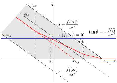
Figure 1: Per-capita demand ($d$, red) and supply ($s$, blue) curves as functions of the price deviation $x$ to be realized in period $t$. A case with $H=3$ types of traders is sketched, where $z_{1,t}$ is the demand of "fundamentalists" (see Sect. 2.4), while $z_{2,t}$ and $z_{3,t}$ are the demands of "non-fundamentalists" ($f_{2}(\mathbf{x}_{t})>0$, $f_{3}(\mathbf{x}_{t})<0$, and negative (dashed) demands are obtained with (7)). The resulting per capita demand curve is piecewise-linear, continuous, and decreasing. Depending on the traders’ fractions ($n_{1,t}$, $n_{2,t}$, $n_{3,t}$), it can take on different configurations in the shaded area (the most negative of which corresponds to $z_{3,t}$ when $n_{3,t}=1$; the case shown corresponds to $n_{1,t}=n_{2,t}=n_{3,t}=1/3$). At the unconstrained price $x_{U,t}$ traders of type $3$ are in a short position in period $t$.

When solving Eq. (2) for $x_{t}$ with the constrained demands (13), $2^{H}-1$ cases must be further distinguished, depending on which of the optimal demands in (7) are forced to zero by (13) (obviously not all demands can vanish). The uniqueness of forward dynamics guarantees that only one of the cases clears the market.

For simplicity, hereafter we will only consider the case with two types of traders ($H=2$), so one of the following three cases is realized at each period:

• no trader is prohibited from going short (equivalently, both types of traders hold nonnegative amounts of shares in period $t$), i.e.,
  (7) implies $z_{1,t}\geq 0$ and $z_{2,t}\geq 0$, with $x_{t}=\displaystyle\frac{\displaystyle 1}{\displaystyle R}\left(n_{1,t}\,f_{1}(\mathbf{x}_{t})+n_{2,t}\,f_{2}(\mathbf{x}_{t})\right)$,

• traders of type $1$ are prohibited from going short (only traders of type $2$ hold shares in period $t$), i.e.,
  (7) implies $z_{1,t}<0$ and $z_{2,t}>0$, with $x_{t}=\displaystyle\frac{\displaystyle 1}{\displaystyle R}\left(f_{2}(\mathbf{x}_{t})-a\hskip 0.56905pt\sigma^{2}s\displaystyle\frac{\displaystyle n_{1,t}}{\displaystyle n_{2,t}}\right)$,

• traders of type $2$ are prohibited from going short (only traders of type $1$ hold shares in period $t$), i.e.,
  (7) implies $z_{1,t}>0$ and $z_{2,t}<0$, with $x_{t}=\displaystyle\frac{\displaystyle 1}{\displaystyle R}\left(f_{1}(\mathbf{x}_{t})-a\hskip 0.56905pt\sigma^{2}s\displaystyle\frac{\displaystyle n_{2,t}}{\displaystyle n_{1,t}}\right)$.

Then, $m_{t+1}$ must be computed (see (11)) and, again, there are three cases, depending on the signs of the optimal demands at period $(t-1)$ (see Eq. (5)). In order to simplify the model formulation, we prefer to enlarge the system’s state, by including the traders’ demands $z_{h,t-1}$ realized in period $(t-1)$, $h=1,2$, in lieu of the farthest price deviation $x_{t-(L+1)}$. The state variables therefore are

$$\makebox[142.26378pt][r]{$(x_{t-1},x_{t-2},\dots,x_{t-L},\ z_{1,t-1},\ z_{2,t-1},\ m_{t})$}\quad\text{if}\quad L\geq 2,$$ (14a)

$$\makebox[142.26378pt][r]{$(x_{t-1},x_{t-2},\ z_{1,t-1},\ z_{2,t-1},\ m_{t})$}\quad\text{if}\quad L=1,$$ (14b)

as we need $x_{t-2}$ to apply the uptick rule, and we can update the traders’ fractions by simply replacing (12) with

$$m_{t+1}=\tanh\left(\displaystyle\frac{\displaystyle\beta}{\displaystyle 2}\left((x_{t}-R\hskip 0.56905ptx_{t-1}+a\hskip 0.56905pt\sigma^{2}s)(z_{1,t-1}-z_{2,t-1})-(C_{1}-C_{2})\right)\right).$$ (15)

The uptick rule makes the ARED model piecewise smooth, namely the space of the state variables is partitioned into three regions associated with different equations for updating the system’s state (see (di Bernardo et al., 2008) and references therein). By defining the regions

$$\begin{array}[]{lrrr}\lx@intercol\hfil U\hfil\lx@intercol:&x_{t-1}>x_{t-2},\\ Z_{0}:&x_{t-1}\leq x_{t-2},&z_{1,t}\geq 0,&z_{2,t}\geq 0,\\ Z_{1}:&x_{t-1}\leq x_{t-2},&z_{1,t}<0,&z_{2,t}>0,\\ Z_{2}:&x_{t-1}\leq x_{t-2},&z_{1,t}>0,&z_{2,t}<0,\par\end{array}$$ (16a)

where

$$z_{1,t}=\displaystyle\frac{\displaystyle 1-m_{t}}{\displaystyle 2}\,\displaystyle\frac{\displaystyle f_{1}(\mathbf{x}_{t})-f_{2}(\mathbf{x}_{t})}{\displaystyle a\hskip 0.56905pt\sigma^{2}}+s\quad\text{and}\quad z_{2,t}=\displaystyle\frac{\displaystyle 1+m_{t}}{\displaystyle 2}\,\displaystyle\frac{\displaystyle f_{2}(\mathbf{x}_{t})-f_{1}(\mathbf{x}_{t})}{\displaystyle a\hskip 0.56905pt\sigma^{2}}+s$$ (16b)

are the optimal demands from (8), we can write the forward dynamics as follows:

$$x_{t} = \left\{\begin{array}[]{ll}\makebox[170.71652pt][l]{$\displaystyle\frac{\displaystyle 1}{\displaystyle 2R}\left((1+m_{t})f_{1}(\mathbf{x}_{t})+(1-m_{t})f_{2}(\mathbf{x}_{t})\right)$}&\quad\text{if}\quad(\mathbf{x}_{t},m_{t})\in U\cup Z_{0},\\[5.69054pt] \displaystyle\frac{\displaystyle 1}{\displaystyle R}\left(f_{2}(\mathbf{x}_{t})-a\hskip 0.56905pt\sigma^{2}s\hskip 0.56905pt\displaystyle\frac{\displaystyle 1+m_{t}}{\displaystyle 1-m_{t}}\right)&\quad\text{if}\quad(\mathbf{x}_{t},m_{t})\in Z_{1},\\[5.69054pt] \displaystyle\frac{\displaystyle 1}{\displaystyle R}\left(f_{1}(\mathbf{x}_{t})-a\hskip 0.56905pt\sigma^{2}s\hskip 0.56905pt\displaystyle\frac{\displaystyle 1-m_{t}}{\displaystyle 1+m_{t}}\right)&\quad\text{if}\quad(\mathbf{x}_{t},m_{t})\in Z_{2},\\[5.69054pt] \end{array}\right.$$ (17d)

$$z_{1,t} = \left\{\begin{array}[]{ll}\makebox[170.71652pt][l]{$\displaystyle\frac{\displaystyle 1-m_{t}}{\displaystyle 2}\,\displaystyle\frac{\displaystyle f_{1}(\mathbf{x}_{t})-f_{2}(\mathbf{x}_{t})}{\displaystyle a\hskip 0.56905pt\sigma^{2}}+s$}&\quad\text{if}\quad(\mathbf{x}_{t},m_{t})\in U\cup Z_{0},\\[5.69054pt] 0&\quad\text{if}\quad(\mathbf{x}_{t},m_{t})\in Z_{1},\\[5.69054pt] \displaystyle\frac{\displaystyle 2\hskip 0.56905pts}{\displaystyle 1+m_{t}}&\quad\text{if}\quad(\mathbf{x}_{t},m_{t})\in Z_{2},\\[5.69054pt] \end{array}\right.$$ (17h)

$$z_{2,t} = \left\{\begin{array}[]{ll}\makebox[170.71652pt][l]{$\displaystyle\frac{\displaystyle 1+m_{t}}{\displaystyle 2}\,\displaystyle\frac{\displaystyle f_{2}(\mathbf{x}_{t})-f_{1}(\mathbf{x}_{t})}{\displaystyle a\hskip 0.56905pt\sigma^{2}}+s$}&\quad\text{if}\quad(\mathbf{x}_{t},m_{t})\in U\cup Z_{0},\\[5.69054pt] \displaystyle\frac{\displaystyle 2\hskip 0.56905pts}{\displaystyle 1-m_{t}}&\quad\text{if}\quad(\mathbf{x}_{t},m_{t})\in Z_{1},\\[5.69054pt] 0&\quad\text{if}\quad(\mathbf{x}_{t},m_{t})\in Z_{2},\\[5.69054pt] \end{array}\right.$$ (17l)

$$m_{t+1} = \tanh\left(\displaystyle\frac{\displaystyle\beta}{\displaystyle 2}\left((x_{t}-R\hskip 0.56905ptx_{t-1}+a\hskip 0.56905pt\sigma^{2}s)(z_{1,t-1}-z_{2,t-1})-(C_{1}-C_{2})\right)\right).$$ (17m)

The same model can be rewritten in compact notations as follows:

$$\left(x_{t},z_{1,t},z_{2,t},m_{t+1}\right) = \left\{\begin{array}[]{ll}\makebox[28.45274pt][l]{$G_{1}\left(\mathbf{x}_{t},z_{1,t-1},z_{2,t-1},m_{t}\right)$}&\quad\text{if}\quad(\mathbf{x}_{t},m_{t})\in U\cup Z_{0},\\[5.69054pt] G_{2}\left(\mathbf{x}_{t},z_{1,t-1},z_{2,t-1},m_{t}\right)&\quad\text{if}\quad(\mathbf{x}_{t},m_{t})\in Z_{1},\\[5.69054pt] G_{3}\left(\mathbf{x}_{t},z_{1,t-1},z_{2,t-1},m_{t}\right)&\quad\text{if}\quad(\mathbf{x}_{t},m_{t})\in Z_{2},\\[5.69054pt] \end{array}\right.$$ (21)

where $G_{1}$, $G_{2}$ and $G_{3}$ are three systems that define the asset pricing model with uptick rule.

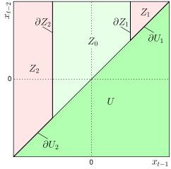
Figure 2: Partition of the state space into the three regions $U\cup Z_{0}$ (green) and $Z_{h}$, $h=1,2$ (pink): the projection on the $(x_{t-1},x_{t-2})$ space in the case where traders use the fundamental and chartist predictors (see Section 2.4).

Region $U\cup Z_{0}$ is separated from region $Z_{h}$, $h=1,2$, by the two boundaries

$$\partial U_{h}:\;x_{t-1}=x_{t-2},\;z_{h,t}\leq 0\quad\text{and}\quad\partial Z_{h}:\;x_{t-1}\leq x_{t-2},\;z_{h,t}=0$$ (23)

(see Figure (2), where a projection on the $(x_{t-1},x_{t-2})$ space is shown). Across boundary $\partial U_{k}$ the system is discontinuous, i.e., the corresponding expressions on the right-hand sides of (17d–c) assume different values on $\partial U_{k}$. In contrast, the system is continuous (but not differentiable) at the boundaries $\partial Z_{h}$.

Similarly to the unconstrained model (10), the initial condition of model (17) is set by the opening price deviation $x_{0}$ and the traders’ initial composition $m_{1}$. However, Eq. (17m) also requires the traders’ demand $z_{1,0}$ and $z_{2,0}$ which can be conventionally set at $s$.

Finally, let’s discuss the fixed points of model (17) (or equivalently (21)), which necessarily lie on the boundary of region $U$ and are still denoted with the pair $(\bar{x},\bar{m})$ (the equilibrium demands, which also characterize the equilibria of model (17), can be obtained from Eqs. (17h,c)). Each of the three systems defining model (17), system $G_{1}$ (equivalent to model (10) adding the demands as state variables) which defines the dynamics of the model in region $U\cup Z_{0}$ and the two systems, $G_{1}$ and $G_{2}$, which define the dynamics of the model in regions $Z_{1}$ and $Z_{2}$, respectively, have their own fixed points, which we call either admissible or virtual according to the region of the state space in which they are. In this paper, a generic fixed point or equilibrium of system $G_{1}$ is called admissible if it lies in region $U\cup Z_{0}$ and virtual otherwise, a generic fixed point of system $G_{2}$ is called admissible if it lies in region $Z_{1}$ and virtual otherwise, and a generic fixed point of system $G_{3}$ is called admissible if it lies in region $Z_{2}$ and virtual otherwise. Virtual fixed points are not equilibria of model (17), but tracking their position is useful in the analysis.

The fundamental equilibrium is always an admissible fixed point of system $G_{1}$, also called the unconstrained system because equivalent to model (10) adding the demands as state variables. Indeed, it lies on the boundary between regions $U$ and $Z_{0}$, with positive demands (equal to $s$), i.e., it is always an interior point of region $U\cup Z_{0}$. Its local stability is therefore ruled by Lemma 1 (the storage of the previous demands in lieu of the farthest past deviation brings the number of zero eigenvalues to $2H-1$, $2H$ if $L=1$, see (14b)), while the existence of (admissible or virtual) non-fundamental equilibria of the unconstrained system $G_{1}$ is ruled by Lemma 2.

The fixed points of the other two systems, $G_{2}$ and $G_{3}$, are of little interest. They lie on the boundaries $\partial U_{2}$ and $\partial U_{1}$, respectively, across which model (17) is discontinuous. Hence, there are arbitrarily small perturbations from the fixed point entering region $U$, for which the unconstrained system $G_{1}$ will map the system’s state far from the fixed point. The fixed points of the two systems $G_{2}$ and $G_{3}$ are therefore (highly) unstable and will not be considered in the analysis.

2.4 Classical price predictors

In this Section we briefly introduce the price predictors used in this paper (see, e.g., (Elder, 1993), (Chiarella and He, 2002), and (Chiarella and He, 2003), for a more complete survey of the most classical types of price predictors used in the literature). The first one, $f_{1}(\mathbf{x}_{t})$, called fundamental predictor, will be paired with each of the others, the non-fundamental predictors, in the analysis of Sections 3 and 4. For this reason, all non-fundamental predictors will be denoted by $f_{2}(\mathbf{x}_{t})$.

Fundamental predictor

Fundamental traders, or fundamentalists, believe that prices return to their fundamental value. The simplest fundamental prediction is the fundamental price for period $t+1$, irrespectively of the recent trend:

$$E_{1}[p_{t+1}]=\bar{p},\quad f_{1}(\mathbf{x}_{t})=0.$$ (24)

More generally, fundamentalists believe that prices will revert to the fundamental value by a factor $v$ at each period:

$$E_{1}[p_{t+1}]=\bar{p}+v\hskip 0.56905pt(p_{t-1}-\bar{p}),\quad f_{1}(\mathbf{x}_{t})=v\hskip 0.56905ptx_{t-1},\quad 0\leq v<1,$$ (25)

the smaller is $v$, the highest is the expected speed of convergence to the fundamental price.

As in (Brock and Hommes, 1998), we assume that "training" costs must be borne to obtain enough "understanding" of how markets work in order to believe in the fundamental price, so fundamentalists incur into a cost $C_{1}>0$ at each prediction.

Chartist predictor

The second type of simple trader that we consider is called chartist or trend chaser. This type of trader believes that any mispricing will continue, i.e. the chartist predictor is formally equivalent to predictor (25):

$$E_{2}[p_{t+1}]=\bar{p}+g\hskip 0.56905pt(p_{t-1}-\bar{p}),\quad f_{2}(\mathbf{x}_{t})=g\hskip 0.56905ptx_{t-1},\quad g>1,$$ (26)

but amplifies, instead of damping, nonzero price deviations from the fundamental.

The chartist prediction is not costly.

Rate of change (ROC) predictor

The third type of simple trader that we consider is called "nonlinear technical analyst" or "ROC trader".

The ROC ("Price Rate Of Change") is a nonlinear prediction which applies the price rate of change averaged over the last $L-1$ periods,

$$\text{ROC}=\left(\displaystyle\frac{\displaystyle p_{t-1}}{\displaystyle p_{t-L}}\right)^{\frac{1}{L-1}}=\left(\displaystyle\frac{\displaystyle\bar{p}+x_{t-1}}{\displaystyle\bar{p}+x_{t-L}}\right)^{\frac{1}{L-1}},\quad L\geq 2,$$ (27a)

to $$p_{t-1} p_{t+1}$$ twice to extrapolate :

$$E_{2}[p_{t+1}]=p_{t-1}\hskip 0.56905pt\text{ROC}^{2},\quad f_{2}(\mathbf{x}_{t})=(\bar{p}+x_{t-1})\hskip 0.56905pt\text{ROC}^{2}-\bar{p}.$$ (27b)

The ROC predictor is typically "smoothed” to avoid extreme rates of change (rates that are either too high or too close to zero, see Smoothed-ROC or S-ROC predictors in (Elder, 1993)). This interprets the traders’ rationality that makes them diffident with extreme rates. We adopt in particular the confidence mechanism introduced in (Dercole and Cecchetto, 2010), where the ROC is combined with the last available price. Precisely, the price rate of change to be applied is a convex combination of the actual ROC (27a) and the unitary rate (corresponding to the last available price), with the ROC weight $$\alpha_{\text{ROC}}$$ that vanishes when the ROC attains extreme values (zero and infinity):

$$E_{2}[p_{t+1}] = p_{t-1}\left(\alpha_{\text{ROC}}\hskip 0.56905pt\text{ROC}+(1-\alpha_{\text{ROC}})\right)^{2},$$

$$f_{2}(\mathbf{x}_{t}) = (\bar{p}+x_{t-1})\left(\alpha_{\text{ROC}}\hskip 0.56905pt\text{ROC}+(1-\alpha_{\text{ROC}})\right)^{2}-\bar{p}.$$ (27c)

The function

$$\alpha_{\text{ROC}}=\displaystyle\frac{\displaystyle 2}{\displaystyle\text{ROC}^{\hskip 1.42262pt\alpha}+\text{ROC}^{\hskip 1.42262pt-\alpha}}$$ (27d)

has been used in the analysis, where the parameter $1/\alpha$ measures how confident traders are with extreme rates.

The ROC predictor and the S-ROC predictor are not costly.

3 The effect of the uptick rule on shares price fluctuations: Analytical results

In this Section we report the stability analysis of fundamental and non-fundamental equilibria of models (12) and (17) for two pairs of traders’ types. As traditionally done in the literature, type $1$ is always the fundamental type (price predictor (25)), while type two is either the chartist in Sect. 3.1 (predictor (26)) or the nonlinear technical analyst (ROC trader) in Sect. 3.2 (predictor (27a,c,d)).

3.1 Fundamentalists vs chartists

Consider models (12) and (17) with predictors (25) and (26). Model (12, 25, 26) is the classical ARED model, proposed and fully analyzed in (Brock and Hommes, 1998) for the case of zero supply of outside shares, i.e., $s=0$, where short selling is intrinsically practiced at each trading period. The case with positive supply is analyzed in (Anufriev and Tuinstra, 2009), where the effects of a negative bound on the traders’ positions are also investigated.

Without any constraint on short selling, the existence and stability of the fixed points of model (12, 25, 26) are defined in the following lemma:

Lemma 3

The following statements hold true for the dynamical system (12) with predictors (25) and (26):

1. For $1<g<R$ the fundamental equilibrium $(0,\bar{m}^{(0)})$ (see Lemma 1) is the only fixed point and is globally stable.

2. For $R<g<2R-v$ there are the following possibilities:

   1. For $0\leq\beta<\beta_{\mathrm{LP}}=\displaystyle\frac{\displaystyle 1}{\displaystyle C}\log\left(\displaystyle\frac{\displaystyle R-v}{\displaystyle g-R}\right)\left(1+\displaystyle\frac{\displaystyle a\hskip 0.56905pt\sigma^{2}s^{2}}{\displaystyle 4C}\displaystyle\frac{\displaystyle g-v}{\displaystyle R-1}\right)^{-1}>0$ the fundamental equilibrium is the only fixed point and is stable.

   2. At $\beta=\beta_{\mathrm{LP}}$ two equilibria appear (as $\beta$ increases) at

      $$\bar{x}_{\mathrm{LP}}=\displaystyle\frac{\displaystyle a\hskip 0.56905pt\sigma^{2}s}{\displaystyle 2(R-1)}>0,\quad\bar{m}=1-2\hskip 0.56905pt\displaystyle\frac{\displaystyle R-v}{\displaystyle g-v},$$

      through a saddle-node bifurcation (limit point, LP).

   3. For $\beta_{\mathrm{LP}}<\beta<\min\left\{\beta_{\mathrm{TR}}=\displaystyle\frac{\displaystyle 1}{\displaystyle C}\log\left(\displaystyle\frac{\displaystyle R-v}{\displaystyle g-R}\right),\beta_{\mathrm{NS}}^{(+)}\right\}>\beta_{\mathrm{LP}}$ the fundamental equilibrium is locally (asymptotically) stable and coexists with the two non-fundamental equilibria $(\bar{x}^{(\pm)},\bar{m})$, with

      $$\bar{x}^{(\pm)}=\bar{x}_{\mathrm{LP}}\pm\sqrt{\left(\bar{x}_{\mathrm{LP}}^{2}+\displaystyle\frac{\displaystyle a\hskip 0.56905pt\sigma^{2}C}{\displaystyle(R-1)(g-v)}\right)\left(1-\displaystyle\frac{\displaystyle\beta_{\mathrm{LP}}}{\displaystyle\beta}\right)}\hskip 0.85358pt.$$

      Equilibrium $(\bar{x}^{(+)},\bar{m})$ is locally (asymptotically) stable, whereas $(\bar{x}^{(-)},\bar{m})$ is a saddle with 2-dimensional stable manifold separating the basins of attraction of the two stable equilibria.

   4. At $\beta=\beta_{\mathrm{TR}}$, $(\bar{x}^{(-)},\bar{m})$ collides and exchanges stability with the fundamental equilibrium (transcritical bifurcation, TR). The fundamental equilibrium is always at least locally (asymptotically) stable for $\beta<\beta_{\mathrm{TR}}$ and it is always unstable for $\beta>\beta_{\mathrm{TR}}$.

   5. At $\beta=\beta_{\mathrm{NS}}^{(+)}$ the equilibrium $(\bar{x}^{(+)},\bar{m})$ undergoes a Neimark-Sacker (NS) bifurcation. No explicit expression is available for $\beta_{\mathrm{NS}}^{(+)}$, but $\beta_{\mathrm{TR}}\lessgtr\beta_{\mathrm{NS}}^{(+)}$ if $\beta_{\mathrm{TR}}\lessgtr\displaystyle\frac{\displaystyle 1}{\displaystyle a\hskip 0.56905pt\sigma^{2}s^{2}}\displaystyle\frac{\displaystyle(R-1)^{2}}{\displaystyle(g-R)(R-v)}$.

   6. For $\beta_{\mathrm{TR}}<\beta<\beta_{\mathrm{NS}}^{(-)}>\beta_{\mathrm{TR}}$ the fundamental equilibrium is a saddle, with 2-dimensional stable manifold separating the positive from the negative dynamics, and the equilibrium $(\bar{x}^{(-)},\bar{m})$, with $\bar{x}^{(-)}<0$, is stable.

   7. At $\beta=\beta_{\mathrm{NS}}^{(-)}$ the equilibrium $(\bar{x}^{(-)},\bar{m})$ undergoes a Neimark-Sacker bifurcation.

3. For $g>2R-v$ there are the following possibilities:

   1. For $0\leq\beta<\beta_{\mathrm{NS}}^{(\pm)}$ the fundamental equilibrium is unstable and the equilibria $(\bar{x}^{(\pm)},\bar{m})$ ($\bar{x}^{(+)}>0$ and $\bar{x}^{(-)}<0$) are stable.

   2. At $\beta=\beta_{\mathrm{NS}}^{(\pm)}$ the equilibria $(\bar{x}^{(\pm)},\bar{m})$ undergo a Neimark-Sacker bifurcation.

4. For $g>R^{2}$ the dynamics can be unbounded for sufficiently large $\beta$.

Lemma 3 generalizes Lemmas 2, 3, and 4 in (Brock and Hommes, 1998) to the case $s>0$, $0<v<1$, and Proposition 3.1 in (Anufriev and Tuinstra, 2009). In particular, for $s=0$, note that the saddle-node and transcritical bifurcations concomitantly occur (case $2$) at a so-called pitchfork bifurcation, whereas the mechanism making the fundamental equilibrium unstable is different for $s>0$. First, the two non-fundamental equilibria $(\bar{x}^{(\pm)},\bar{m})$ appear (as the traders’ adaptability $\beta$ increases) through the saddle-node bifurcation, and as $\beta$ increases further a transcritical bifurcation occurs in which the saddle $(\bar{x}^{(-)},\bar{m})$ exchanges stability with the fundamental equilibrium. Thus, for $\beta_{\mathrm{LP}}<\beta<\beta_{\mathrm{TR}}$, the fundamental equilibrium is stable, but coexists with an alternative stable fixed point of model (12, 25, 26).

With the uptick-rule, the existence and stability of the fixed points of model (17, 25, 26) are complemented by the following lemma:

Lemma 4

The following statements hold true for the dynamical system (17) with predictors (25) and (26):

1. The local and global stability of the fundamental equilibrium is as in Lemma 3. As long as equilibria $(\bar{x}^{(\pm)},\bar{m})$ exist and are admissible, their local stability is as in Lemma 3. Equilibrium $(\bar{x}^{(+)},\bar{m})$ is admissible iff $\bar{x}^{(+)}\leq\bar{x}_{\mathrm{BC}}^{(+)}=a\hskip 0.56905pt\sigma^{2}s/(R-v)$. Equilibrium $(\bar{x}^{(-)},\bar{m})$ is admissible iff $\bar{x}_{\mathrm{BC}}^{(-)}=-a\hskip 0.56905pt\sigma^{2}s/(g-R)\leq\bar{x}^{(-)}\leq\bar{x}_{\mathrm{BC}}^{(+)}$.

2. For $R<g<2R-v$ there are the following possibilities:

   1. If $R+v>2$, equilibria $(\bar{x}^{(\pm)},\bar{m})$ appear admissible at $\beta=\beta_{\mathrm{LP}}$ and $(\bar{x}^{(+)},\bar{m})$ becomes virtual (border-collision bifurcation) at $\beta=\beta_{\mathrm{BC}}^{(+)}$, with

      $$0<\beta_{\mathrm{BC}}^{(+)}=\displaystyle\frac{\displaystyle 1}{\displaystyle C}\log\left(\displaystyle\frac{\displaystyle R-v}{\displaystyle g-R}\right)\left(1+\displaystyle\frac{\displaystyle a\hskip 0.56905pt\sigma^{2}s^{2}}{\displaystyle C}\displaystyle\frac{\displaystyle(g-v)(1-v)}{\displaystyle(R-v)^{2}}\right)^{-1}<\beta_{\mathrm{TR}}.$$

   2. If $R+v<2$, equilibria $(\bar{x}^{(\pm)},\bar{m})$ appear virtual at $\beta=\beta_{\mathrm{LP}}$ and $(\bar{x}^{(-)},\bar{m})$ becomes admissible at $\beta=\beta_{\mathrm{BC}}^{(+)}$.

   3. If $R+v=2$, equilibria $(\bar{x}^{(\pm)},\bar{m})$ appear on the border $\partial Z_{1}$ at $\beta=\beta_{\mathrm{LP}}=\beta_{\mathrm{BC}}^{(+)}$ and $(\bar{x}^{(+)},\bar{m})$ and $(\bar{x}^{(-)},\bar{m})$ are respectively virtual and admissible for larger $\beta$.

   4. If $s<s_{\mathrm{BC}}^{(-)}=\left(\displaystyle\frac{\displaystyle C}{\displaystyle a\hskip 0.56905pt\sigma^{2}}\displaystyle\frac{\displaystyle(g-R)^{2}}{\displaystyle(g-v)(g-1)}\right)^{1/2}$, equilibrium $(\bar{x}^{(-)},\bar{m})$ becomes virtual at $\beta=\beta_{\mathrm{BC}}^{(-)}$, with

      $$\beta_{\mathrm{BC}}^{(-)}=\displaystyle\frac{\displaystyle 1}{\displaystyle C}\log\left(\displaystyle\frac{\displaystyle R-v}{\displaystyle g-R}\right)\left(1-\displaystyle\frac{\displaystyle a\hskip 0.56905pt\sigma^{2}s^{2}}{\displaystyle C}\displaystyle\frac{\displaystyle(g-v)(g-1)}{\displaystyle(g-R)^{2}}\right)^{-1}>\beta_{\mathrm{TR}}.$$

3. For $g>2R-v$ there are the following possibilities:

   1. If $s<s_{\mathrm{BC}}^{(-)}$ equilibria $(\bar{x}^{(\pm)},\bar{m})$ are virtual for any $\beta\geq 0$.

   2. If $s>s_{\mathrm{BC}}^{(-)}$ equilibrium $(\bar{x}^{(+)},\bar{m})$ is virtual for any $\beta\geq 0$, whereas $(\bar{x}^{(-)},\bar{m})$ is admissible for $\beta>\beta_{\mathrm{BC}}^{(-)}>0$.

4. For $g>R^{2}$ the dynamics can be unbounded for sufficiently large $\beta$.

Note that the uptick rule affects the price dynamics also when the supply of outside shares is large. Indeed, independently on $s$, there is always an equilibrium, $(\bar{x}^{(+)},\bar{m})$ or $(\bar{x}^{(-)},\bar{m})$, becoming virtual as $\beta$ increases or decreases.

3.2 Fundamentalists vs ROC traders

Consider models (12) and (17) with the fundamental predictor (25) and with the ROC predictor (27a,b) or (27a,c,d).

Note that both predictors are such that $f_{h}(\bar{x}\mathbf{1})/\bar{x}<R$ for any possible equilibrium $(\bar{x},\bar{m})$ with $\bar{x}\neq 0$, so by means of Lemma 2 the fundamental equilibrium is the only fixed point. In the simplest case $L=2$, its stability is characterized in the following lemma:

Lemma 5

The following statements hold true for the dynamical systems (12) and (17) with predictors (25) and (27a,b), as well as with predictors (25) and (27a,c,d):

1. For $R\geq 2$ the fundamental equilibrium $(0,\bar{m}^{(0)})$ (see Lemma 1) is a stable fixed point for any $\beta>0$.

2. For $R<2$ the fundamental equilibrium is stable for

   $$0<\beta<\beta_{\mathrm{NS}}=\displaystyle\frac{\displaystyle 1}{\displaystyle C}\log\left(\displaystyle\frac{\displaystyle R}{\displaystyle 2-R}\right)$$

   and loses stability through a Neimark-Sacker bifurcation at $\beta=\beta_{\mathrm{NS}}$.

Similarly to the cases where chartists are paired with fundamentalists (Sect. 3.1), the stability of the fundamental equilibrium is guaranteed if the gross return $R$ is sufficiently large.

The stability analysis for $L>2$ is possible, following the lines indicated in (Kuruklis, 1994), and the general conclusion is that rates of change calculated on larger windows of past prices stabilize the fundamental equilibrium, up to the point that the fixed point is stable for any value of $\beta$ if $L$ is sufficiently large.

4 The effect of the uptick rule on share price fluctuations: Numerical simulations.

In the first two Subsections of this Section we report several numerical analysis of models (12) and (17) for the two pairs of traders’ types considered in Sect. 3, with the aim of characterizing the non-stationary (periodic, quasi-periodic, or chaotic) asymptotic regimes. This part contains technical considerations. In the last subsection, we discuss the effects of the uptick rule on the price dynamics.

As done in most of the related works in the literature, we use the traders’ adaptability (or intensity of choice) $\beta$ as a bifurcation parameter (two- or higher-dimensional bifurcation analyses are possible, see, e.g., (Dercole and Cecchetto, 2010), but will not be considered here). For each considered value of $\beta$, the transient dynamics is eliminated by computing the (largest) Lyapunov exponent associated to the orbit, i.e., we delete the number of initial iterations required to compute the largest Lyapunov exponent, whereas the asymptotic regime is discussed. To graphically study the bifurcations underwent by the different attractors, we vertically plot the deviations $x_{t}$ in the attractor at the corresponding value of $\beta$, together with the associated largest Lyapunov exponent L (see, e.g., Figure (3)).

In each simulation, we set the initial condition as follows. The opening price deviation $x_{0}$ is randomly selected in a small, positive or negative neighborhood of zero to study the stability of the fundamental equilibrium; far from zero to study non-fundamental attractors. The initial traders’ fractions are equally set ($m_{1}=0$, i.e., $n_{1,1}=n_{2,1}=1/2$). For model (17), the initial values assigned to the traders’ demands $z_{1,0}$ and $z_{2,0}$ are irrelevant, as the traders’ fractions are not updated at $t=1$.

4.1 Fundamentalists vs chartists

We first study the effects of a positive supply of outside shares ($s>0$) on the dynamics of the original model (12, 24, 26) introduced by (Brock and Hommes, 1998), then we study the effects of the uptick rule. Figure (3) reports the bifurcation diagrams and the corresponding largest Lyapunov exponent obtained for four different values of $s$ (with $s$ in the range of values commonly used in the literature, see (Anufriev and Tuinstra, 2009; Hommes et al., 2005)). The first panel is the case with zero supply of outside shares ($s=0$) and is included for comparison.

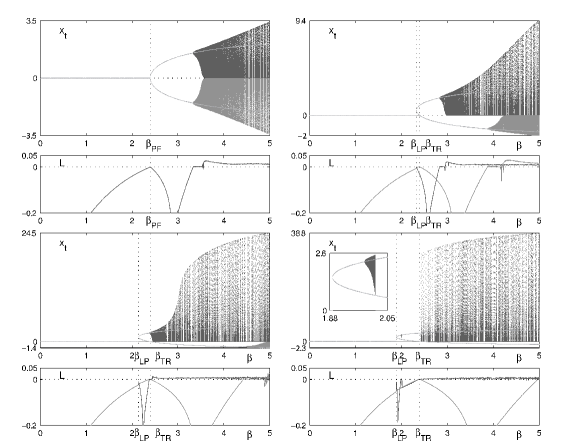
Figure 3: Bifurcation diagrams of model (12, 24, 26) for different values of $s$ (the supply of outside shares of the risky asset): A (first row, left column) $s=0$, in this case $\beta_{\mathrm{TR}}=\beta_{\mathrm{LP}}=\beta_{\mathrm{PF}}$, related (largest) Lyapunov exponents in (second row, left column); B (first row, right column) $s=0.1$, in this case $\beta_{\mathrm{TR}}<\beta_{\mathrm{NS}}^{(+)}$, related (largest) Lyapunov exponents in (second row, right column); C (third row, left column) $s=0.2$, in this case $\beta_{\mathrm{TR}}=\beta_{\mathrm{NS}}^{(+)}$, related (largest) Lyapunov exponents (fourth row, left column); D (third row, right column) $s=0.3$, in this case $\beta_{\mathrm{TR}}>\beta_{\mathrm{NS}}^{(+)}$, related (largest) Lyapunov exponents (fourth row, right column). $\beta_{\mathrm{NS}}^{(+)}$ and $\beta_{\mathrm{NS}}^{(-)}$ are not ticked because there is no analytical expression for them. However, the Neimark-Sacker bifurcation values can be clearly identified in the bifurcation diagrams. Other parameter values: $R=1.1$, $a=1$, $\sigma=1$, $\bar{y}=1$, $g=1.2$, $C=1$.

The bifurcation points $\beta_{\mathrm{LP}}$, $\beta_{\mathrm{TR}}$, and $\beta_{\mathrm{NS}}$ are indicated, together with the non-fundamental equilibria $(\bar{x}^{(\pm)},\bar{m})$ (the gray parabola), and are in agreement with the analytical results of Lemma 3. In particular, $\beta_{\mathrm{LP}}=\beta_{\mathrm{TR}}=\beta_{\mathrm{PF}}$ indicates a pitchfork bifurcation when $s=0$.

Note that the positive and negative deviation dynamics are separated in model (12, 24, 26). Indeed, due to the characteristics of the chartist predictor (26), if the opening price is above [below] the fundamental value ($x_{0}>0$ [$x_{0}<0$]), it will remain so forever (see Eq. (12a)). The positive and negative attractors therefore coexist (with basins of attraction separated by the linear manifold $x_{t-1}=0$ in state space), so that two Lyapunov exponents (one for each of the two attractors) are plotted.

As expected, the fundamental equilibrium is destabilized for sufficiently high traders’ adaptability and the amplitude of the price fluctuations increases as $\beta$ increases. But the amplitude of fluctuations also increases with the supply of outside shares of the risky asset $s$ (note the different vertical scales in Figure (3)). The latter effect is partially due to the risk premium, i.e. $\left(a\sigma^{2}s\right)$, required by traders for holding extra shares that modifies the performance measures of the trading strategies.

Figure (3) shows another interesting dynamical phenomenon. For sufficiently high supply of outside shares of the risky asset ($s=0.3$ in case D), the positive attractor, that appears at the Neimark-Sacker (NS) bifurcation ($\beta_{\mathrm{NS}}^{(+)}$) of equilibrium $(\bar{x}^{(+)},\bar{m})$, collapses through a "homoclinic” contact with the saddle equilibrium $(\bar{x}^{(-)},\bar{m})$. The chaotic behavior is then reestablished when the fundamental equilibrium looses stability through the transcritical bifurcation ($\beta_{\mathrm{TR}}$).

The analysis of the dynamics conducted up to now reveals that there are not substantial differences in the price dynamics for different values ​​of $s$, except the amplitude of price fluctuations and some peculiar phenomena, such as the homoclinic contact just discussed. For this reason and to make the discussion more clear and concise, in the following we investigate the effects of the uptick rule on the price dynamics only for $s=0.1$.

Figure (4) compares models (12) (left) and (17) (right) with predictors (24) and (26). The bifurcation diagram and the largest Lyapunov exponents associated with the different attractors are reported, together with two examples of state portraits (projections in the plane $(x_{t},x_{t-1})$, see bottom panels). Blue and red dots identify the points in the attractor in which respectively fundamentalists and chartists have been prohibited from going short.

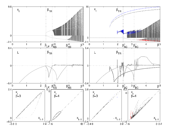
Figure 4: Bifurcation diagrams of models (12, 24, 26) (left) and (17, 24, 26) (right) and exemplary state portraits projections in the plane $(x_{t},x_{t-1})$. Parameter values as in Figure (3)-case(B). The light gray represents the attractor of negative deviations and the corresponding largest Lyapunov exponent. The dark gray represents the attractor of positive deviations and the corresponding largest Lyapunov exponent. The black represents the attractor born through a nonsmooth saddle-node bifurcation and the corresponding largest Lyapunov exponent. The blue dots indicate that fundamentalists cannot have negative positions because of the uptick rule. The red dots indicate that chartists cannot have negative positions because of the uptick rule.

The first thing to remark is that multiple positive attractors are present in the constrained dynamics (right column in Figure (4)), i.e. when the uptick rule is in place. In particular a period-two cycle alternating unrestricted trading with restricted trading in which fundamentalists are forced by the uptick rule to take nonnegative positions (black and blue dots) is present for sufficiently large $\beta$. It appears through a nonsmooth saddle-node bifurcation and coexists with the chaotic attractor generated through the loss of fundamental stability. Before the bifurcation the fundamental equilibrium is globally stable (while it is globally stable in the unconstrained dynamics up to the saddle-node at $\beta=\beta_{\mathrm{LP}}$).

Also the bifurcation structure leading to the chaotic attractor is more involved. The first branch of attractors suddenly appears as $\beta$ increases. This is probably due to a homoclinic contact with the period-two saddle cycle, but this conjecture has not been verified. This first branch seems to collapse through a collision with the border $\partial Z_{1}$, in connection with the border collision of the non-fundamental equilibrium $(\bar{x}^{(+)},\bar{m})$ at $\beta=\beta_{\mathrm{BC}}^{(+)}$. The remaining thinner attractor later explodes into a larger one, again due to a border collision with $\partial Z_{1}$. However, a deeper mathematical investigation would be required to confirm the above conjectures.

As for the negative equilibrium $(\bar{x}^{(-)},\bar{m})$ (for $\beta>\beta_{\mathrm{TR}}$), it loses stability at $\beta=\beta_{\mathrm{BC}}^{(-)}$ through a border collision with $\partial Z_{2}$, giving way to a chaotic attractor characterized by restrictions on chartists.

Figure (5) shows an example of time series on the positive chaotic attractor obtained for $\beta=3$ (left column: unconstrained dynamics; right column: dynamics constrained by the uptick rule).

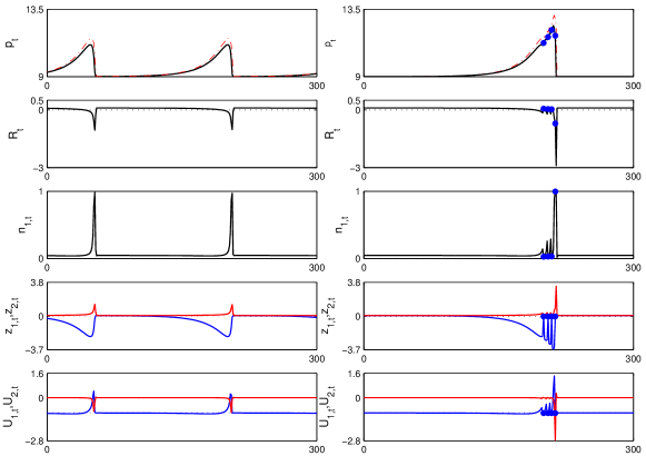
Figure 5: Positive (i.e. above fundamental) time series on the asymptotic regime of models (12, 24, 26) (left) and (17, 24, 26) (right) for $\beta=3$. Other parameter values as in Figure (3)-case(B). The blue dots indicate that fundamentalists cannot have negative positions because of the uptick rule.

The top panels report the price dynamics (black) and the chartist prediction (red, dashed), with blue and red dots marking the periods in which fundamentalists and chartists are respectively prevented to go short by the uptick rule (right column). The remaining panels report, from top to bottom, the returns ($R_{t}=x_{t}-R\hskip 0.56905ptx_{t-1}+a\hskip 0.56905pt\sigma^{2}s$) and the traders’ fractions ($n_{h,t}$), demands ($z_{h,t}$), and net profits ($U_{h,t}=R_{t}z_{h,t-1}-C_{h}$, $h=1,2$, blue for fundamentalists and red for chartists).

The price dynamics is characterized by recurrent peaks (financial bubbles), driven by chartists that expect a price rise and hold the shares of the risky asset and, at the same time, attenuated by fundamentalists which expect a devaluation and sell short (see the negative positions of fundamentalists in the unconstrained dynamics, left). In particular, when the price is closed to its fundamental value, the chartists’ trading strategy is more profitable because their expectations are confirmed. Chartists dominate the market and the price is growing until the capital gain cannot compensate for the lower dividend yield. At this point, chartists start to suffer negative returns, while the short positions of the fundamentalists produce profits. Eventually most of traders adopt the fundamentalist’s trading strategy and the price falls down close to the fundamental value. As soon the price starts to revert to the fundamental value, however, fundamentalists are prohibited from going short in the constrained dynamics because of the uptick rule (right column), and this triggers a further phase of rising prices. This happens several times, with the result of amplifying the price peak. At a certain point, when the price is very far away from its fundamental value, chartists suffer strong losses and the relative fraction of fundamentalists is almost one. The massive presence of fundamentalists pushes the price close to its fundamental value and the uptick rule cannot prevent this from happening. Indeed, if there are almost only fundamentalists, from the pricing equation we have that their demands must be equal to the supply of outside share, i.e. positive. When the price is close to its fundamental price chartists start to have a better performance and the story repeats. Despite this mispricing effect, the frequency of the price peaks is slowed down by the short selling restriction.

Similarly, Figure (6) shows an example of time series on the negative attractor obtained for $\beta=4$ (here the unconstrained dynamics is quasi-periodic, see Figure (4)).

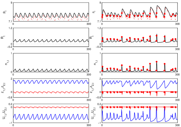
Figure 6: Negative (i.e., below fundamental) time series on the asymptotic regime of models (12, 24, 26) (left) and (17, 24, 26) (right) for $\beta=4$. Other parameter values as in Figure (3)-case(B). The red dots indicate that chartists cannot have negative positions because of the uptick rule.

In this case of negative price deviations, the chartists go short and have, on average, higher profits than fundamentalists. In the unconstrained dynamics chartists are predominant and drive prices down. This phenomenon is attenuated by the uptick rule, which limit the downward price movements and increases the performance of fundamentalists. The frequencies of the negative peaks is slightly lowered by the short selling restriction, but they are more irregular due to the presence of chaotic dynamics as indicated by the positivity of the largest Lyapunov exponent, see Figure (4).

The different types of price dynamics, quasi-periodic for the unconstrained model and chaotic for the constrained one, are due to the different types of bifurcations through which the non-fundamental equilibrium $(\bar{x}^{(-)},\bar{m})$ losses stability, a Neimark-Sacker bifurcation in the first case and a border-collision bifurcation in the second. Indeed, as typical in piecewise linear model, at the border-collision bifurcation we have sudden transition from a stable fixed point to a fully developed robust (i.e., without periodic windows) chaotic attractor, see, e.g. (di Bernardo et al., 2008).

4.2 Fundamentalists vs ROC traders

Figure (7) reports the bifurcation analysis of models (12) (left) and (17) (right) with predictors (24) and (27a,c,d), while Figure (8) shows the time series on the chaotic attractor obtained for $\beta=1.4$.

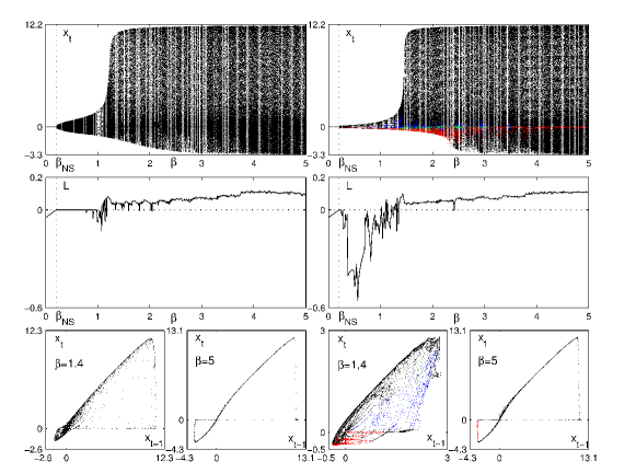
Figure 7: Bifurcation diagrams of models (12, 24, 27a,c,d) (left) and (17, 24, 27a,c,d) (right) and exemplary state portraits projections in the plane $(x_{t},x_{t-1})$. Parameter values: $\alpha=10$, $L=2$, other values as in Figure (3)-case(B). The blue dots indicate that fundamentalists cannot have negative positions because of the uptick rule. The red dots indicate that chartists cannot have negative positions because of the uptick rule.

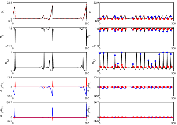
Figure 8: Time series on the asymptotic regime of models (12, 24, 27a,c,d) (left) and (17, 24, 27a,c,d) (right) for $\beta=1.4$. Other parameter values as in Figure (7). The blue dots indicate that fundamentalists cannot have negative positions because of the uptick rule. The red dots indicate that chartists cannot have negative positions because of the uptick rule.

Here the fundamental equilibrium is globally stable up to the Neimark-Sacker bifurcation at $\beta\leq\beta_{\mathrm{NS}}$. Interestingly, the price fluctuations showed by the non-stationary attractors originated for larger $\beta$ (quasi-periodic with periodic windows and later chaotic) have a remarkably smaller amplitude in the constrained dynamics, than in the unrestricted case. In this sense, the uptick-rule shows a rather robust stabilizing effect, at least as long $\beta$ is not too large, i.e., traders are not fast enough in changing their beliefs to react to past performances.

This is also evident in the time series of Figure (8), where the short selling restriction also intensifies the frequency of the price peaks.

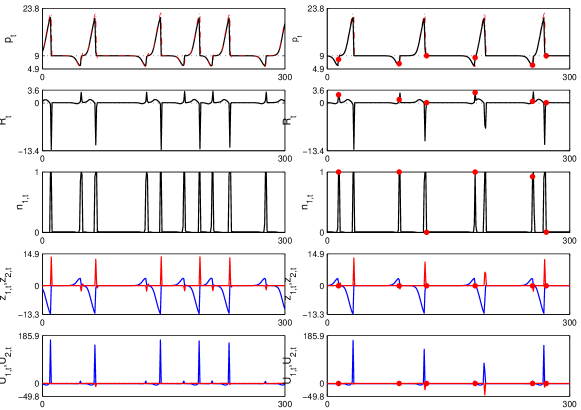
Figure 9: Time series on the asymptotic regime of models (12, 24, 27a,c,d) (left) and (17, 24, 27a,c,d) (right) for $\beta=4.5$. Other parameter values as in Figure (7). The red dots indicate that chartists cannot have negative positions because of the uptick rule.

4.3 Economic discussion of the numerical results

On the basis of the three declared objectives of the uptick rule, this subsection provides a discussion of the effects of this short selling regulation in the light of the analytical and by numerical analysis reported in the previous Sections.

Let us start to discuss the scenario described by models (12) and (17) with predictors (25) and (26) (fundamentalists vs chartists). We first consider the case of negative price deviations (the negative attractor in Figure (4) and the time series in Figure (6)), where we see that chartists take short positions when prices fall, whereas fundamentalists take long positions believing that the stock price will rise to reach the fundamental value (see the unconstrained dynamics in the left column of Figure (6)). It is important to point out that whenever an asset is undervalued (price below its fundamental value) it should be better to hold it rather than to sell it because the return is always positive: dividend yield outweighs the capital gain effect. Indeed, by going short chartists obtain negative excess returns, see the dynamic of the net profits $U_{2,t}$ in the last row of Figure (6). However chartists do better than fundamentalists here because the latter are charged a cost, $\left(C\right)$, which is larger than the profit they obtain by holding the assets, compare the net profits of the two trading strategies ($U_{1,t}$ and $U_{2,t}$) again in the last row of Figure (6). It follows that chartists are predominant in the market, as indicated by the low value of the fraction $n_{1}$, and their trading strategy causes downward movements of the stocks’ price. In the constrained dynamics (right column), the uptick rule limits the possibility to go short for chartists. This helps to revert the stock prices toward the fundamental value. It follows a better performance for the fundamentalists and their presence in the market increases. As a result, the short selling restriction reduces the negative peaks reached by stock prices. From this example it is clear the effectiveness of the regulation to meet the last two goals established by the SEC. Moreover, from the analysis of the bifurcation diagram, it is interesting to note that the negative non-fundamental equilibrium $(\bar{x}^{(-)},\bar{m})$ looses stability in the constrained dynamics at a lower traders’ adaptability, i.e., at a lower value of the parameter $\beta$, respect to the unconstrained dynamics. This is due to the border collision bifurcation at $\beta=\beta_{\mathrm{BC}}^{(-)}$, that occurs before the Neimark-Sacker bifurcation at $\beta_{\mathrm{NS}}^{(-)}$ responsible of the instability in the unconstrained dynamics. This might be mathematically interpreted as a destabilizing effect of the uptick rule. However, the chaotic fluctuations established after the bifurcation move the prices, on average, closer to the fundamental value with respect to the equilibrium deviation $\bar{x}^{(-)}$.

Considering the same model and predictors, by the time series of Figure (5) it is possible to notice that the dynamics of positive price deviations are characterized (for $\beta>\beta_{\mathrm{NS}}^{(+)}$) by frequently financial bubbles. These bubbles are enforced by chartists which overvalued the stock prices in the upward trend and are attenuated by fundamentalists. In fact, in these phases of rising prices fundamentalists go short driven by the belief that the price will revert to its fundamental value in the next period. This increases the supply of shares helping to curb rising prices. At a certain point of the upward trend, the fundamentalists’ strategy take over and prices are driven to the fundamental value of the stock. During these upward trends of the market the uptick rule prevents the fundamentalists to take short positions, see blue dots in the fourth row, right column of Figure (5). This phenomenon is also emphasized by empirical analysis (see, e.g., (Alexander and Peterson, 1999) and (Boehmer et al., 2008)), and represents a flaw of the regulation. The result is an increase of the amplitude of the financial bubbles. As a positive effect of the regulation, it is possible to notice a reduction in the frequency of occurrences of these bullish divergences.

The main point is that every time fundamentalists go short they force prices to converge to the fundamental value. If it were possible to discriminate between the beliefs of the traders, fundamentalists should not be forbidden to go short in this situation. However, this is a very difficult task and it is not even so easy to correctly determine the fundamental values of a risky asset in the real market. A possible solution could be to allow short sales after a long period of rising prices. This should avoid pushing up prices because fundamentalists (and contrarians, but these traders are not taken into consideration in this work) are driven out of the market. Another possible solution could be to restrict short selling only in cases of sharp and sudden falls in stock prices. This should produce two effects, to let agents believing in the fundamental price go short when the price increases, reducing positive oscillations of price deviations from the fundamental value, and to reduce sharp drops in prices observed when the stock market bubble breaks. An important step in this direction has already been done, the SEC adopted Rule 201 which was implemented on February 28, 2011. This new short selling regulation prohibits short selling operations if the value of the stock decreases by more than 10% in two consecutive trading sections.

Summarizing the analysis of the positive and negative price deviations from the fundamental value for the model with predictors (24) and (26) for the cases of unrestricted and restricted short sales, we can conclude that the second goal of the regulation is ensured, but some distorting effects produced by this rule are observed, such as overvaluation of shares. Moreover, the short selling restriction can trigger distorting mechanisms that support dynamics of overpricing, otherwise not feasible in the long run. This is indicted by the presence of multiple attractors in the region of positive price deviations in the bifurcation diagram in the right column of Figure (4).

With the intent to provide a more detailed and comprehensive description of the effects of the uptick rule, the same asset pricing model has been analyzed with a different non-fundamental predictor (the Smoothed-ROC predictor, see Subsection 2.4). Differently from other trend-following indicators, the Smoothed-ROC predictor is particularly useful to detect fast and short-term upward and downward movements of the stock price and gives different trading signals to agents than predictor (26), such as gain and lose of speed in the trend (see (Elder, 1993)). In this case, we obtain an interesting and surprising result, i.e., the uptick rule helps to reduce the amplitude of price fluctuations, and causes an increase of the frequency of oscillations above and below the fundamental value, this is made clear by comparing the time series of prices in the first row of Figure (8). The explanation of this lies on the higher degree of rationality (compared to the one assumed for chartists) of the non-fundamentalist agents that the use of the non-linear predictor (S-ROC predictor) implies. These agents are uncomfortable with extreme assessments of the value of the shares and when the shares are forced to be overvalued due to the short selling constraints, non-fundamental agents react and become more confidential in the fundamental price. This changes their trading strategies and, as a results, the amplitude of the price fluctuations decreases instead of increasing as might be expected. The choice of the value of $\alpha$ plays an important rule in this. We can conclude that by using this couple of predictors it is possible to observe, at least when evolutionary pressure, $\beta$, is not excessively large, all the main goals of the uptick rule: short selling restriction does not produce mispricing, prevents chartists from going short during downward price movements to avoid reaching negative price variation peaks and prevents fundamentalists from going short only in a downward price movement for positive price deviations, reducing the speed of convergence to the fundamental value and preventing sharps drops in prices. As a further observation, it is worth noticing that the uptick rule prevents extremely negative excess returns and at the same time makes the strategy of fundamentalists on the average more profitable, changing the beliefs of traders, compare $n_{1,t}$ and $n_{2,t}$ in Figure (8). Moreover, looking at the bifurcation diagram of Figure (7) right-column, it is clear that for relatively high values of the intensity of choice, $\beta$, the uptick rule does not have any effect on the amplitude of price fluctuations. As revealed by the analysis of the time series in Figure (9), this is due to the fact that for high levels of $\beta$ the market is always dominated by one trading strategy. It follows that the short selling constraint can apply either to a trading strategy adopted almost by any trader or to a trading strategy adopted by almost all the traders. In the first case the regulation does not have any effect on the price, in the second case it reverts the price toward the fundamental value with the results of reducing the frequency of market-bubbles but without reducing the amplitude of them. Compare the two panels in the first row of Figure (9). For $\beta$ large enough, at each trading section there is only one type of trader that dominates the market and its demand of shares, being equal to the supply of outside share per trader, must be positive, then the uptick rule does not affect the dynamics of prices.

The conducted analysis points out that the uptick rule meets part of its goals, but which of them often depends on the condition of the markets. Moreover, the regulation can produce several side-effects which may be different according once again to the market’s conditions and investor’s beliefs which may strongly influence the effectiveness of the regulation itself. Due to these findings, studying the impact of the uptick rule on financial markets does not seem to be an easy task. Nonetheless, it is possible to isolate some remarkable effects regardless of market conditions and traders’ beliefs. First, the uptick rule ensures a reduction of the downward market movements when the shares are undervalued, i.e. when the shares are priced below their fundamental value. Second, the intensity of choice $\beta$ to switch predictors affects the effectiveness of the short selling regulation. By using the bifurcation analysis, it possible to observe that the effectiveness of the regulation fades away increasing the value of $\beta$ (increasing $\beta$, agents tend to overreact to the market’s information, changing their beliefs quickly to react to past performances). In other words, the switching destabilizing effect prevails over the regulation’s effects, i.e. when agents overreact to the differences in performance related to different beliefs, the regulation does not affect the dynamics of stock prices. This is consistent with many interesting empirical results testifying that there is no statistical effect of the uptick rule on price fluctuations in turbulent financial markets (see, e.g., (Diether et al., 2009)).

As a final remark, it is important to clarify that the simple asset pricing model used in this paper can reproduce only some possible “stylized effects” which are a direct consequence of the regulation. However, in the real financial markets many more different trading strategies and emotional actions are present, which can modify the effectiveness of the uptick rule.

5 Conclusions and future directions

In this paper, we have investigated the effect of the "uptick rule" on an asset price dynamics by means of an asset pricing model with heterogeneous, adaptive beliefs. The analysis has suggested the effectiveness of the regulation in reducing the downward price movements of undervalued shares avoiding speculative behavior whenever the market is characterized by not too many aggressive traders, i.e. when the agents’ propensity of changing trading strategy is relatively low. On the contrary, when the agents have a high propensity of changing trading strategy according to the past trading performances, which is a sign of turbulent markets according to the model, the effects of the regulation tend to fade. As a side effect of the regulation, an amplification of the market bubbles in the case of overvalued shares is possible.

This work represents only a starting point. There are still several aspects that can and deserve to be analyzed. First of all, it is interesting to analyze the effect of the uptick regulation using the same asset pricing model with a greater number of investor types, for example contrarians, chartists and fundamentalists. In fact, there is empirical evidence in the literature about the switch in trading style by short-sellers. (Diether et al., 2009) found that under the uptick rule most of the short positions are opened by contrarians, on the contrary, when the uptick rule is not imposed are chartists, the ones who prefer to go short (see, e.g., (Boehmer et al., 2008)). There is a hypothetical explanation for this. Chartists take short positions in declining price trends and the uptick rule makes this operation more difficult, on the contrary the restriction does not effect the contrarians’ short strategy. They usually go short in upward price trend betting on a change in price movement with the effect of stabilizing the market. Investigating the validity of this hypothesis provides a better understanding of the issue.

The regulation should also be evaluated in the contest of the multi-assets market to discover how the short selling restriction for one stock influences the price of the others. It is reasonable to expect that traders will switch to trade stocks that are not effected by the restriction in that specific moment and this can produce effects on prices which are not easy to predict without a deep analysis.

Another aspect that deserves to be investigated is the effect of the regulation when there is a fraction of investors which does not change the trading strategy (or belief) as in (Dieci et al., 2006). As highlighted in this paper, the uptick rule loses its effectiveness due to a high propensity to switch trading strategy by agents. It follows that, if there are constraints on the possibility to change trading strategy, we expect an increase of the effectiveness of the regulation and a reduction of unwelcome effects on price dynamics. Last but not least, the piecewise continuous model here proposed can be easily adapted according to the new short selling regulation imposed by the SEC, i.e. Rule 201. Comparing the two cases can help to understand the pros and cons of the new regulation.

6 Appendix

Proof of Lemma 1. The existence of the fundamental equilibrium immediately follows by substituting $f_{h}(\mathbf{0})=0$ into Eqs. (10) and (12). For the definition of the associated eigenvalues, let us substitute Eq. (10) written for $n_{h,t}$ into Eq. (10a) (and Eq. (12) written for $m_{t}$ into Eq. (12a)). Then, we can consider $(x_{t-1},\ldots,x_{t-(L+2)})$ as the state variables for both models, and the Jacobian of the system at the fundamental equilibrium is equal to

$$\left[\begin{array}[]{c|c}\begin{array}[]{ccccc}\gamma_{1}&\hskip 11.38109pt\gamma_{2}&\cdots&&\gamma_{L}\\ 1&0&\cdots&&0\\ 0&1&\cdots&&0\\ \vdots&&\ddots&&0\\ 0&0&\cdots&\hskip 14.22636pt1&0\end{array}&\begin{array}[]{ccc}\hskip 2.84526pt0&&\hskip 2.84526pt0\\ 0&&0\\ 0&&0\\ \vdots&&\vdots\\ 0&&0\end{array}\\ \hline\cr\begin{array}[]{ccccc}0&\hskip 11.38109pt0&\cdots&\hskip 14.22636pt0&\hskip 5.69054pt1\\ 0&\hskip 11.38109pt0&\cdots&\hskip 14.22636pt0&\hskip 5.69054pt0\end{array}&\begin{array}[]{ccc}\hskip 2.84526pt0&&\hskip 2.84526pt0\\ 1&&0\end{array}\end{array}\right],$$

which proves the result.   

Proof of Lemma 2. At the equilibrium price deviation $\bar{x}$, we obviously have $\mathbf{x}_{t}=\bar{x}\mathbf{1}$ and, from Eq. (10a), $\bar{x}$ must satisfy

$$R=\sum_{h=1}^{H}n_{h,t}\hskip 0.56905ptf_{h}(\bar{x}\mathbf{1})/\bar{x}.$$

Being $n_{h,t}\in(0,1)$ for all $h=1,\ldots,H$, this is possible only if $f_{h}(\bar{x}\mathbf{1})/\bar{x}<R$ for some $h$ and $f_{k}(\bar{x}\mathbf{1})/\bar{x}>R$ for some $k\neq h$.   

Proof of Lemma 3.

1. The uniqueness follows from Lemma 2, while the global stability from (12a), which can be rewritten as

   $$x_{t}=\displaystyle\frac{\displaystyle 1}{\displaystyle R}\left(n_{1,t}\hskip 0.56905ptv+n_{2,t}\hskip 0.56905ptg\right)x_{t-1},$$

   and contracts the deviation $x_{t}$ as $t$ goes to infinity.

2. From Lemma 1, the non-zero eigenvalue associated to the fundamental equilibrium is

   $$\lambda^{(0)}=\gamma_{1}=\displaystyle\frac{\displaystyle 1}{\displaystyle 2R}\left((1+\bar{m}^{(0)})\hskip 0.56905ptv+(1-\bar{m}^{(0)})\hskip 0.56905ptg\right)>0,\quad\bar{m}^{(0)}=\tanh\left(-\beta\hskip 0.56905ptC/2\right).$$

   Thus the fundamental equilibrium can loose stability only when $\lambda^{(0)}=1$ at a transcritical (or pitchfork) bifurcation (being fixed point of model (12, 25, 26) for any admissible parameter setting, it cannot disappear through a saddle-node bifurcation). Solving $\lambda^{(0)}=1$ for $\beta$ gives $\beta_{\mathrm{TR}}$.

   Evaluating Eqs. (10) at the generic equilibrium $(\bar{x},\bar{m})$, solving Eq. (12a) for $\bar{m}$, and equating the result to Eq. (12), we get

   $$\bar{m}=1-2\hskip 0.56905pt\displaystyle\frac{\displaystyle R-v}{\displaystyle g-v}=\tanh\left(-\displaystyle\frac{\displaystyle\beta}{\displaystyle 2}\left((-(R-1)\hskip 0.56905pt\bar{x}+a\hskip 0.56905pt\sigma^{2}s)\hskip 0.56905pt\displaystyle\frac{\displaystyle g-v}{\displaystyle a\hskip 0.56905pt\sigma^{2}}\hskip 0.56905pt\bar{x}+C\right)\right),$$

   which solved for $\bar{x}$ gives $\bar{x}^{(\pm)}$.

   Solving $\bar{x}^{(+)}=\bar{x}^{(-)}$ for $\beta$ gives $\beta_{\mathrm{LP}}$ and the equilibrium deviations $\bar{x}^{(\pm)}$ are defined only for $\beta>\beta_{\mathrm{LP}}$. There are therefore no other equilibria and this concludes the proof of points (a), (LP), and (TR). Note that $\beta_{\mathrm{LP}}=\beta_{\mathrm{TR}}$ when $s=0$ (the transcritical and saddle-node bifurcations coincide at a pitchfork bifurcation).

   Substituting Eq. (12) written for $m_{t}$ into Eq. (12a) and using $(x_{t-1},x_{t-2},x_{t-3})$ as state variables, the Jacobian of the systems at equilibria $(\bar{x}^{(\pm)},\bar{m})$ is given by

   $$\left[\begin{array}[]{ccc}\gamma_{1}^{(\pm)}&\gamma_{2}^{(\pm)}&\gamma_{3}^{(\pm)}\\ 1&0&0\\ 0&1&0\end{array}\right],$$

   with

   $$\gamma_{1}^{(\pm)}=1+\displaystyle\frac{\displaystyle\gamma}{\displaystyle R}\hskip 0.56905pt\bar{x}^{(\pm)},\quad\gamma_{2}^{(\pm)}=-\gamma\hskip 0.56905pt\bar{x}^{(\pm)},\quad\gamma_{3}^{(\pm)}=\displaystyle\frac{\displaystyle\gamma}{\displaystyle R}\left(-(R-1)\hskip 0.56905pt\bar{x}^{(\pm)}+a\hskip 0.56905pt\sigma^{2}s\right),$$

   and

   $$\gamma=\beta\hskip 0.56905pt\bar{x}^{(\pm)}\displaystyle\frac{\displaystyle(g-v)^{2}}{\displaystyle 4\hskip 0.56905pta\hskip 0.56905pt\sigma^{2}}\hskip 1.42262pt\mathrm{sech}^{2}\left(-\displaystyle\frac{\displaystyle\beta}{\displaystyle 2}\left((-(R-1)\hskip 0.56905pt\bar{x}^{(\pm)}+a\hskip 0.56905pt\sigma^{2}s)\hskip 0.56905pt\displaystyle\frac{\displaystyle g-v}{\displaystyle a\hskip 0.56905pt\sigma^{2}}\hskip 0.56905pt\bar{x}^{(\pm)}+C\right)\right),$$

   so the three associated eigenvalues $\lambda_{1}$, $\lambda_{2}$, $\lambda_{3}$ are the roots of the characteristic equation

   $$\lambda^{3}-\gamma_{1}^{(\pm)}\lambda^{2}-\gamma_{2}^{(\pm)}\lambda-\gamma_{3}^{(\pm)}=0.$$

   In particular, imposing $\lambda=1$ and solving the characteristic equation for $\bar{x}^{(\pm)}$, gives only zero and $x_{\mathrm{LP}}$ as solutions, so no other transcritical, saddle-node (or pitchfork) bifurcation is possible. In contrast, imposing $\lambda_{1}=-1$ and taking into account that $\lambda_{1}+\lambda_{2}+\lambda_{3}=\gamma_{1}$, we get $\lambda_{2}+\lambda_{3}=2+\gamma\hskip 0.56905pt\bar{x}^{(\pm)}/R>2$ (note that $\gamma\hskip 0.56905pt\bar{x}^{(+)}>0$ and that $\gamma\hskip 0.56905pt\bar{x}^{(-)}\geq 0$ only vanishes at the transcritical bifurcation), so that equilibrium $(\bar{x}^{(\pm)},\bar{m})$ would be unstable at a period-doubling (flip) bifurcation. However, both equilibria $(\bar{x}^{(\pm)},\bar{m})$ loose stability by increasing $\beta$, because the coefficient $\gamma_{1}$ linearly diverges with $\beta$ (the limit as $\beta\to\infty$ of the $\mathrm{sech}$ argument is finite and equal to $-\log((R-v)/(g-R))/2<0$), so the same does the sum of the eigenvalues. Stability is therefore lost through a Neimark-Sacker bifurcation and this concludes the proof of points (b), (c), and (NS^(±)).

3. For $g>2R-v$, the non-zero eigenvalue $\lambda^{(0)}$ associated to the fundamental equilibrium is larger than one for any $\beta>0$. We also have $\beta_{\mathrm{LP}}<0$, $\beta_{\mathrm{TR}}<0$, and equilibria $(\bar{x}^{(\pm)},\bar{m})$ are defined for any $\beta>0$ with $\bar{x}^{(+)}>0$ and $\bar{x}^{(-)}<0$. Similarly to point 2, they loose stability through a Neimark-Sacker bifurcation.

4. In the limiting case $\beta\to\infty$, from Eq. (12) we have

   $$m_{t+1}=\left\{\begin{array}[]{rl}1&\text{if}\quad(R\hskip 0.56905ptx_{t-1}-x_{t}-a\hskip 0.56905pt\sigma^{2}s)\displaystyle\frac{\displaystyle g-v}{\displaystyle a\hskip 0.56905pt\sigma^{2}}x_{t-1}>C,\\ -1&\text{if}\quad(R\hskip 0.56905ptx_{t-1}-x_{t}-a\hskip 0.56905pt\sigma^{2}s)\displaystyle\frac{\displaystyle g-v}{\displaystyle a\hskip 0.56905pt\sigma^{2}}x_{t-1}<C.\end{array}\right.$$

   Starting at $x_{0}=\pm\epsilon$ with sufficiently small $\epsilon>0$ and $m_{1}=-1$, we therefore have $x_{t}=\pm\epsilon(g/R)^{t}$ (see Eq. (12a)) as long as $m_{t+1}$ stays at $-1$. Thus, $x_{t}$ diverges if

   $$\epsilon^{2}(g/R)^{2t-1}\left(\displaystyle\frac{\displaystyle R^{2}}{\displaystyle g}-1\mp a\hskip 0.56905pt\sigma^{2}s\hskip 0.56905pt\epsilon^{-1}(g/R)^{-t}\right)\displaystyle\frac{\displaystyle g-v}{\displaystyle a\hskip 0.56905pt\sigma^{2}}>C,$$

   is never satisfied for increasing $t$, i.e., when $g>R^{2}$.

 

Proof of Lemma 4.

1. At the fundamental equilibrium, the traders’ demands are positive ($\bar{z}^{(0)}_{1}=\bar{z}^{(0)}_{2}=s$), so $(0,\bar{m}^{(0)})$ is an admissible fixed point of the unconstrained dynamics for any admissible parameter setting. Its local stability is therefore ruled by Lemma 3.

   The global stability for $1<g<R$ is a consequence of the following arguments. First, the price deviation is contracted from period $(t-1)$ to period $t$ (i.e., $|x_{t}|<|x_{t-1}|$) whenever the unconstrained dynamics is applied (see Lemma 3, point 1). Second, the unconstrained deviation $x_{t}^{(0)}$ following $x_{t-1}$ is smaller than any of the constrained deviations $x_{t}^{(1)}$ and $x_{t}^{(2)}$ given by Eq. (17d) in region $Z_{1}$ and $Z_{2}$, respectively. This is graphically clear from Figure (1), and is analytically shown by noting that

   $$x_{t}^{(h)}-x_{t}^{(0)}=-\displaystyle\frac{\displaystyle a\hskip 0.56905pt\sigma^{2}}{\displaystyle R}\hskip 0.56905pt\displaystyle\frac{\displaystyle n_{h}}{\displaystyle n_{k}}\hskip 0.56905ptz_{h,t}^{(0)}>0,\quad h=1,2,\;k\neq h$$

   (see (16b), and recall that $z_{h,t}^{(0)}<0$ in region $Z_{h}$). Third, from Eq. (17d) we get that $0<x_{t}^{(0)}<x_{t}^{(h)}<(g/R)x_{t-1}$ when $x_{t-1}>0$ and $x_{t}^{(0)}<x_{t}^{(h)}<(v/R)x_{t-1}<0$ when $x_{t-1}<0$. Thus, the constrained dynamics in regions $Z_{1}$ and $Z_{2}$ also contracts the price deviation from period $(t-1)$ to period $t$.

   Being $\bar{x}^{(+)}>0$, equilibrium $(\bar{x}^{(+)},\bar{m})$ can only collide with border $\partial Z_{1}$ (see (23)), at which $\bar{x}^{(+)}=\bar{x}_{\mathrm{BC}}^{(+)}$ (the expression for $\bar{x}_{\mathrm{BC}}^{(+)}$ can be easily obtained by solving the first equation in (16b) with $z_{1,t}^{(0)}=0$ for $x_{t-1}$). It is obviously admissible iff $\bar{x}^{(+)}\leq\bar{x}_{\mathrm{BC}}^{(+)}$.

   Depending on the parameter setting, equilibrium $(\bar{x}^{(-)},\bar{m})$ can be either positive or negative, and can therefore collide with both borders $\partial Z_{1}$ and $\partial Z_{2}$. At the border $\partial Z_{2}$, $\bar{x}^{(-)}=\bar{x}_{\mathrm{BC}}^{(-)}$ (the expression for $\bar{x}_{\mathrm{BC}}^{(-)}$ is obtained by solving the second equation in (16b) with $z_{2,t}^{(0)}=0$ for $x_{t-1}$), so that $(\bar{x}^{(-)},\bar{m})$ is admissible iff $\bar{x}_{\mathrm{BC}}^{(-)}\leq\bar{x}^{(-)}\leq\bar{x}_{\mathrm{BC}}^{(+)}$.

2. If $R+v>2$ (case (a)), $\bar{x}_{\mathrm{LP}}$ from Lemma 3 is smaller than $\bar{x}_{\mathrm{BC}}^{(+)}$, so that equilibria $(\bar{x}^{(\pm)},\bar{m})$ are admissible at the saddle-node bifurcation. The price deviation $\bar{x}^{(+)}$ increases as $\beta$ increases and reaches $\bar{x}_{\mathrm{BC}}^{(+)}$ at $\beta=\beta_{\mathrm{BC}}^{(+)}$ (collision with border $\partial Z_{1}$). If $R+v<2$ (case (b)), equilibria $(\bar{x}^{(\pm)},\bar{m})$ are virtual at the saddle-node bifurcation. The price deviation $\bar{x}^{(-)}$ decreases as $\beta$ increases and reaches $\bar{x}_{\mathrm{BC}}^{(+)}$ at $\beta=\beta_{\mathrm{BC}}^{(+)}$. If $R+v=2$ (case (c)), then $\beta_{\mathrm{BC}}^{(+)}=\beta_{\mathrm{LP}}$.

   Equilibrium $(\bar{x}^{(-)},\bar{m})$ collides with the border $\partial Z_{2}$ only if the limit of $\bar{x}^{(-)}$ as $\beta\to\infty$ is below $\bar{x}_{\mathrm{BC}}^{(-)}$. This yields the condition on $s$ and the border collision at $\beta=\beta_{\mathrm{BC}}^{(-)}$ in point (d).

3. For $g>2R-v$, $\bar{x}^{(+)}$ increases as $\beta$ increases, whereas $\bar{x}^{(-)}$ decreases, and their limiting value for $\beta\to\infty$ are as in point 2. Equilibrium $(\bar{x}^{(+)},\bar{m})$ is always virtual, because its limiting value is above $\bar{x}_{\mathrm{BC}}^{(+)}$ for any admissible parameter setting. Equilibrium $(\bar{x}^{(-)},\bar{m})$ becomes admissible at $\beta=\beta_{\mathrm{BC}}^{(-)}$ only if its limiting value is above $\bar{x}_{\mathrm{BC}}^{(-)}$, which gives the conditions at points (a) and (b).

4. In the limiting case $\beta\to\infty$, $m_{t}$ switches between $\pm 1$, so that only one type of trader is present and the three options in Eq. (17d) give the same price deviation $x_{t}$. The result therefore follows from Lemma 3.

 

Proof of Lemma 5. From Lemma 1, the characteristic equation associated with the nontrivial eigenvalues of the fundamental equilibrium is $\lambda^{2}-\gamma_{1}\lambda-\gamma_{2}=0$, with

$$\gamma_{1}=\displaystyle\frac{\displaystyle 1}{\displaystyle 2R}\left((1+\bar{m}^{(0)})\hskip 0.56905ptv+3(1-\bar{m}^{(0)})\right),\quad\gamma_{2}=-\displaystyle\frac{\displaystyle 1}{\displaystyle R}\hskip 0.56905pt(1-\bar{m}^{(0)}).$$

Note that the same characteristic equation is obtained for both predictors (27a,b) and (27a,c,d), and also for different choices of the confidence function (27d), as long as $\mathrm{\partial}\hskip 0.56905pt\alpha_{\text{ROC}}/\mathrm{\partial}\hskip 0.56905pt\text{ROC}|_{\text{ROC}=1}=0$.

The fundamental equilibrium is stable at $\beta=0$ (the Routh-Hurwitz-Jury test for 2nd-order polynomials requires $-\gamma_{2}|_{\beta=0}=1/R<1$ and $\gamma_{1}|_{\beta=0}=(v+3)/(2R)<1-\gamma_{2}|_{\beta=0}=(R+3+R-1)/(2R)$, which are readily satisfied).

As $\beta$ increases, transcritical and saddle-node (or pitchfork) bifurcations are not possible. In fact, substituting $\lambda_{1}=1$ into the constraints:

$$\lambda_{1}+\lambda_{2}=\gamma_{1},\quad\lambda_{1}\lambda_{2}=-\gamma_{2},$$

and eliminating $\lambda_{2}$, we get the contradiction

$$R=\displaystyle\frac{\displaystyle v}{\displaystyle 2}\hskip 0.56905pt(1+\bar{m}^{(0)})+\displaystyle\frac{\displaystyle 1}{\displaystyle 2}\hskip 0.56905pt(1-\bar{m}^{(0)})$$

(with left-hand side larger than one and right-hand side smaller than 1).

Similarly, we exclude flip bifurcations: imposing $\lambda_{1}=-1$ in the above constraints and eliminating $\lambda_{2}$, we get the contradiction

$$-R=\displaystyle\frac{\displaystyle v}{\displaystyle 2}\hskip 0.56905pt(1+\bar{m}^{(0)})+\displaystyle\frac{\displaystyle 5}{\displaystyle 2}\hskip 0.56905pt(1-\bar{m}^{(0)}).$$

(with left-hand side positive and right-hand side negative).

To look for a Neimark-Sacker bifurcation, we impose $\lambda_{1}\lambda_{2}=1$ and $|\lambda_{1}\lambda_{2}|<2$. Under the first condition, the second turns into $v\hskip 0.56905pt(1+\bar{m}^{(0)})<R$ that is always satisfied (recall that $\bar{m}^{(0)}<0$, see Lemma 1). Solving the first condition for $\beta$ gives $\beta_{\mathrm{NS}}$.

References

- Alexander and Peterson [1999] G. J. Alexander and M. A. Peterson. Short Selling on the New York Stock Exchange and the Effects of the Uptick Rule. Journal of Financial Intermediation, 8(1-2):90–116, 1999.
- Alligood et al. [1997] K. T. Alligood, T. D. Sauer, and J. A. Yorke. Chaos: An Introduction to Dynamical Systems. Springer, New York, 1997.
- Anufriev and Tuinstra [2009] M. Anufriev and J. Tuinstra. The impact of short-selling constraints on financial market stability in a model with heterogeneous agents. CeNDEF working paper, pages 1–30, 2009.
- Boehmer et al. [2008] E. Boehmer, C. M. Jones, and X. Zhang. Unshackling short sellers: the repeal of the uptick rule. Columbia Business School working paper, pages 1–38, December 2008.
- Bris et al. [2007] A. Bris, W. N. Goetzmann, and N. Zhou. Efficiency and the bear: Short sales and markets around the world. The Journal of Finance, 62(3):1029–1079, 2007.
- Brock and Hommes [1998] W. A. Brock and C. H. Hommes. Heterogeneous beliefs and routes to chaos in a simple asset pricing model. Journal of Economic Dynamics and Control, 22(8–9):1235–1274, 1998.
- Chiarella and He [2002] C. Chiarella and X-Z He. Heterogeneous Beliefs, Risk and Learning in a Simple Asset Pricing Model. Computational Economics, 19(1):95–132, 2002.
- Chiarella and He [2003] C. Chiarella and X-Z He. Dynamics of beliefs and learning under -processes – the heterogeneous case. Journal of Economic Dynamics and Control, 27(3):503–531, 2003.
- Colombo et al. [2012] A. Colombo, M. di Bernardo, S. J. Hogan, and M. R. Jeffrey. Bifurcations of piecewise smooth flows: Perspectives, methodologies and open problems. Physica D: Nonlinear Phenomena, 241(22):1845 – 1860, 2012.
- Dercole and Cecchetto [2010] F. Dercole and C. Cecchetto. A new stock market model with adaptive rational equilibrium dynamics. In Proceedings of COMPENG 2010, IEEE Conference on complexity in engineering, Rome, pages 129–131, 2010.
- di Bernardo et al. [2008] M. di Bernardo, C. J. Budd, A. R. Champneys, and P. Kowalczyk. Piecewise-smooth Dynamical Systems: Theory and Applications. Springer-Verlag, Berlin, 2008.
- Diamond and Verrecchia [1987] D. W. Diamond and R. E. Verrecchia. Constraints on short-selling and asset price adjustment to private information. Journal of Financial Economics, 18(2):277–311, 1987.
- Dieci et al. [2006] R. Dieci, I. Foroni, L. Gardini, and X-Z He. Market mood, adaptive beliefs and asset price dynamics. Chaos, Solitons & Fractals, 29(6):520–534, 2006.
- Diether et al. [2009] K. B. Diether, K.H. Lee, and I. M. Werner. Short-Sale Strategies and Return Predictability. The Review of Financial Studies, 22(2):575–607, 2009.
- Elder [1993] A. Elder. Trading for a living: psychology, trading tactics, money management, volume 31. John Wiley & Sons, 1993.
- Gaunersdorfer [2000] A. Gaunersdorfer. Endogenous fluctuations in a simple asset pricing model with heterogeneous agents. Journal of Economic Dynamic and Control, 24(5-7):799–831, 2000.
- Gaunersdorfer [2001] A. Gaunersdorfer. Adaptive beliefs and the volatility of asset prices. Central European Journal of Operations Research, 9(1–2):5–30, 2001.
- Gaunersdorfer et al. [2008] A. Gaunersdorfer, C. H. Hommes, and F. O. O. Wagener. Bifurcation routes to volatility clustering under evolutionary learning. Journal of Economic Behavior & Organization, 67(1):24–47, 2008.
- Harrison and Kreps [1978] J. M. Harrison and D. M. Kreps. Speculative Investor Behavior in a Stock Market with Heterogeneous Expectations. The Quarterly Journal of Economics, 92(2):323–336, 1978.
- Hommes [2001] C. H. Hommes. Financial markets as nonlinear adaptive evolutionary systems. Quantitative Finance, 1(1):149–167, 2001.
- Hommes et al. [2005] C. H. Hommes, H. Huang, and D. Wang. A robust rational route to randomness in a simple asset pricing model. Journal of Economic Dynamics and Control, 29(6):1043–1072, 2005.
- Hull [2011] J. C. Hull. Options, Futures and Other Derivatives. Prentice Hall, New Jersey, 8th edition, 2011.
- Kuruklis [1994] S. A. Kuruklis. The asymptotic stability of . Journal of Mathematical Analysis and Applications, 188(3):719–731, 1994.
- Miller [1977] E. M. Miller. Risk, Uncertainty, and Divergence of Opinion. The Journal of Finance, 32(4):1151–1168, 1977.
- Misra et al. [2012] V. Misra, M. Lagi, and Y. Bar-Yan. Evidence of market manipulation in the financial crisis. New England Complex Systems Institute (Working Paper), 2012.
- Murphy [1999] J. J. Murphy. Technical Analysis of the Financial Markets: A Comprehensive Guide to Trading Methods and Applications. New York Institute of Finance, New York, 1999.
- Nelly [1997] C. J. Nelly. Technical analysis in the foreign exchange market: a layman’s guide. Federal Reserv Bank of St. Louis Review, pages 23–28, 1997.
- Taylor and Allen [1992] M. P. Taylor and H. Allen. The use of technical analysis in the foreign exchange market. Journal of International Money and Finance, 11(3):304–314, 1992.
- Tramontana and Westerhoff [2013] F. Tramontana and F. Westerhoff. One-dimensional discontinuous piecewise-linear maps and the dynamics of financial markets. Springer-Verlag, Bischi G.I., Chiarella C., Sushko I, Global Analysis of Dynamic Models in Economics and Finance edition, 2013.
- Tramontana et al. [2010a] F. Tramontana, L. Gardini, and F. Westerhoff. Intricate Asset Price Dynamics and One-Dimensional Discontinuous Maps. Nova Science, Puu T., Panchuk A., Nonlinear Economic Dynamics edition, 2010a.
- Tramontana et al. [2010b] F. Tramontana, F. Westerhoff, and L. Gardini. On the complicated price dynamics of a simple one-dimensional discontinuous financial market model with heterogeneous interacting traders. Journal of Economic Behavior & Organization, 74(3):187–205, 2010b.
- Tramontana et al. [2011] F. Tramontana, L. Gardini, and F. Westerhoff. Heterogeneous Speculators and Asset Price Dynamics: Further Results from a One-Dimensional Discontinuous Piecewise-Linear Map. Computational Economics, 38(3):329–347, 2011.
- Westerhoff [2001] F. H. Westerhoff. Speculative behavior, exchange rate volatility, and central bank intervention. Central European Journal of Operations Research, 9(1–2):31–50, 2001.