Can dynamical synapses produce true self-organized criticality?

Abstract

Neuronal networks can present activity described by power-law distributed avalanches presumed to be a signature of a critical state. Here we study a random-neighbor network of excitable cellular automata coupled by dynamical synapses. The model exhibits a very similar to conservative self-organized criticality (SOC) models behavior even with dissipative bulk dynamics. This occurs because in the stationary regime the model is conservative on average, and, in the thermodynamic limit, the probability distribution for the global branching ratio converges to a delta-function centered at its critical value. So, this non-conservative model pertain to the same universality class of conservative SOC models and contrasts with other dynamical synapses models that present only self-organized quasi-criticality (SOqC). Analytical results show very good agreement with simulations of the model and enable us to study the emergence of SOC as a function of the parametric derivatives of the stationary branching ratio.

1 Introduction

In the past few decades there has been an increasing exploration of the heuristic idea that the concepts of complexity and criticality are intermingled [1, 2, 3, 4, 5]. Criticality is associated with critical $d$-surfaces in parameter space, for example, a critical point ($d=0$-surface) or a critical line ($d=1$) in a continuous phase transition. If the system has a $D$-dimensional parameter space, to be critical at a $d<D$ surface necessarily implies fine tuning of the system parameters to be close to that surface. Since several complex systems seem to lie spontaneously at the border of such critical surfaces, we need to explain such fine tuning.

Several mechanisms have been proposed to do that, the most popular being based in the notion of Self-Organized Criticality (SOC). SOC in microscopically conservative systems, whose prototypical example is the sandpile model [3], is by now a well understood issue [6, 7, 8]. The case of non-conservative (bulk) dynamics has also been subjected to intense study and the present consensus is that these systems are critical only in the conservative limit [9, 10, 11, 12, 6, 13, 14, 15, 16, 17]. In the absence of that, what one observes is simply a large critical region surrounding the critical point, which can be confounded with a generic critical interval due to finite size effects (Pseudo-SOC) [11, 12, 6, 13, 14]. Another class of models has loading mechanisms that make the system hover around the critical point [9, 18], with fluctuations that do not vanish in the thermodynamic limit, a case which has been called Self-Organized quasi-Criticality (SOqC) [15, 16]. A review about SOC applied to neural networks discuss several limitations of the present models [19].

Here we introduce a new class of models that, although non-conservative microscopically, after a transient achieves a stationary regime which is conservative on average, with vanishing fluctuations in the thermodynamic limit. This new behavior, not seen in previous SOC models, is due to an intra-avalanche ultra-soft loading mechanism (loading in a slower time scale than that presented in SOqC models). Another advantage of our model is that it has a very simple, exact and transparent mean-field treatment, in comparison to other models of the literature.

2 The model

First we introduce the Levina-Herrmann-Geisel (LHG) model [18, 16], which directly inspired our model. Surprisingly, we will find that the models pertain to different universality classes. In the LHG model the basic excitable elements are integrate-and-fire neurons with time dependent membrane potentials $0<V_{i}(t)<V_{max},i=1,\ldots,N$. The synapses are denoted as $J_{ij}(t)$ and also evolve in time. The synaptic coupling is all-to-all (so there are $N(N-1)$ synapses). The model dynamics is given by

$$\frac{\partial V_{i}}{\partial t}=I^{ext}\delta(t-t^{i}_{driv})+\sum_{j=1}^{N-1}\frac{uJ_{ij}}{N-1}\delta(t-t_{sp}^{j})-V_{max}\delta(t-t_{sp}^{i}),$$ (1)

$$\frac{\partial J_{ij}}{\partial t}=\frac{1}{\tau_{J}}\left(\frac{\alpha}{u}-J_{ij}\right)-uJ_{ij}\delta(t-t_{sp}^{j}).$$ (2)

• Driving: the $I^{ext}$ term is a slow drive on neuron $i$ that acts on times $t^{i}_{driv}$ with a given rate.

• Firing: the neuron spikes if $V_{i}(t)>V_{max}$, which defines the spike time $t_{sp}^{i}$. The term $-V_{max}\delta(t-t_{sp}^{i})$ corresponds to a reset of the membrane potential.

• Integration: the sum over $J_{ij}$ corresponds to the integration, by the postsynaptic neuron $i$, of the synaptic contributions of all firing presynaptic neurons $j$.

• Synaptic depression: when a presynaptic neuron $j$ fires (which defines the spike time $t_{sp}^{j}$), all synapses (out-links) $J_{ij}$ are depressed by the amount $uJ_{ij}$.

• Synaptic recovery: synapses recover to a target value $\alpha/u$ with a time scale given by $\tau_{J}$.

Both LHG [18] and Bonachela et al. [16] did not study the full parameter space $(\alpha,u,\tau_{J},V_{max})$ but mainly studied the effect of varying $\alpha$ with other parameters fixed as $u=0.2,V_{max}=1$ and $\tau_{J}=10N$. They found a critical-like region around $\alpha=1.4$. However, Bonachela et al. showed that this region is pseudocritical because the system’s behavior is an oscillation around the critical point with an amplitude that does not vanish in the large $N$ limit.

Our model builds upon a random-neighbor network of excitable neurons used previously [20] (inspired on the well-known SIRS epidemiological model). The possible states ($S_{i}=0$, $i=1,\dots,N$) are:

• Susceptible or Quiescent: $S_{i}=0$;

• Infected or Firing: $S_{i}=1$ ;

• Recovering or Refractory: $S_{i}=2,3,\ldots,n-1$.

The network is of random neighbor type, each presynaptic neuron $j$ having exactly $K$ outlinks to postsynaptic neurons $i$ described by probabilistic couplings (synapses) $P_{ij}$. Firing sites can induce firing in neighbors sites, creating an avalanche (defined as a not interrupted sequence of firing sites). The dynamics is composed by the following steps:

• Driving: After an avalanche occurs and all sites are either quiescent or refractory, we choose a single site at random and force it to fire ($S_{i}=1$), creating a new avalanche.

• Firing: the probability that a presynaptic neighbor $j$ does not induce a firing in the postsynaptic neuron $i$ is $\left[1-P_{ij}\delta(S_{j}(t),1)\right]$, where henceforth $\delta$ is the Kronecker delta function. So, the probability that a quiescent ($S_{i}(t)=0$) site spikes ($S_{i}(t+1)=1$) is given by $1-\prod_{j=1}^{K_{i}}\left[1-P_{ij}\delta(S_{j}(t),1)\right]$, where $K_{i}$ is the number of incoming links of site $i$ (note that $\langle K_{i}\rangle=K$).

• Refractory time: after a site spikes, it deterministically becomes refractory for $n-2$ time steps, and then returns to quiescence:

  $$S_{i}(t+1)=\left\{\begin{array}[]{ll}S_{i}(t)+1,\textrm{ if }S_{i}=1,2,\ldots,n-2;\\ 0,\textrm{ if }S_{i}=n-1.\end{array}\right.$$ (3)

• Synaptic depression and recovery: to be described below.

Each site has a local branching ratio $\sigma_{i}\equiv\sum_{j}^{K}P_{ij}$ and we can define a global branching ratio $\sigma\equiv N^{-1}\sum_{i}^{N}\sigma_{i}$. If $\{P_{ij}\}$ are drawn from a uniform distribution with average $\sigma/K$ and kept fixed then the average branching ratio $\sigma$ controls the collective behavior of the network: for $\sigma<1$ $(>1)$ the system is subcritical (supercritical), with unstable (self-sustained) activity. This is the static version of the model, without dynamical synapses, which undergoes a continuous absorbing state phase transition at $\sigma=\sigma_{c}=1$ [20]. For this static model, criticality is only achieved by fine tuning $\sigma$ to a critical value $\sigma_{c}$. This absorbing continuous phase transition pertains to the class of Compact Directed Percolation (CDP) and is identical to that present in canonical conservative SOC models [7, 8, 15].

Here we report new results obtained with a homeostatic synaptic mechanism described by time-dependent probabilities $P_{ij}(t)$ that follow a depressing/recovering synaptic dynamics similar to that used in the LHG model [18, 16]. The crucial difference with respect to their model, however, is that the recovering mechanism of our synaptic dynamics occurs at a slower, $O(1/N)$, time scale:

$$P_{ij}(t+1)=P_{ij}(t)+\frac{\epsilon}{NK}(A-P_{ij})-uP_{ij}(t)\delta(t,t^{j}_{sp})\;,$$ (4)

where $t^{j}_{sp}$ is the spiking time of the $j$-th presynaptic neuron. A comparison with the synaptic part of the LHG model (Eq. 2) gives that $\frac{\epsilon}{NK}$ is proportional to $\frac{1}{\tau_{J}}$ (remember that $\tau_{J}$ is proportional to $N$) and that $A=\alpha/u$, with $u$ having the same meaning in both models. The parameters of Eq. 4 can be better understood in Figure 1.

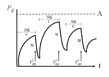
Figure 1: Schematic illustration of Eq. 4 parameters. $P_{ij}$ represents the amount of available neurotransmitters at the synapse between the neurons j and i (in the model, it is the probability of neuron j excites neuron i). The parameter A corresponds to the largest value the synapses can reach; the factor $\epsilon/NK$ is the speed with which synapses recover each time step; and the parameter $u$ is the subtracted fraction of $P_{ij}$ when the presynaptic neuron j fires, it is, when $t=t^{j}_{sp}$.

Notice that the dynamics in $P_{ij}(t)$ leads to a time-dependent global branching ratio $\sigma(t)=\frac{\sum_{ij}P_{ij}}{NK}$. The different time scale from the LHG model arises because they use an all-to-all coupling where synapses already have a scale $1/N$ (like in the all-to-all Ising model). So, synaptic recovery in the LHG model perturbs the synapses with a term of same order $O(1/N)$ and this could be the origin of the large variance on the average synaptic weight measured in [16]. In our case, $P_{ij}$ is $O(1)$ and the $1/N$ factor in Eq. (4) defines an ultra-soft recovery mechanism. Although this could be considered a small modeling change, it produces an important change in the universality class of our model.

We observe that the scaling $1/N$ in the synapses dynamics, also present in the LHG model, is somewhat problematic from the biological point of view, since synapses do not have information about how many neurons there are in the network. However, in the literature of networks with dynamical links, this feature corresponds to the modeling state of art and there are no models without this feature. Perhaps, in real networks, the recovery dynamics mediated by $\epsilon$ does not depend on $N$ but has anyway a very large recovery time (small $\epsilon$) which is sufficient to put the system in a state very close of the critical one. This problem also suggests a research topic: what are the time scales that biological synapses recover after spike and if the recovery time depends on the size of the network.

We also observe that $\sigma(t)=N^{-1}\sum_{ij}^{K}P_{ij}(t)$ is a property of the architecture, and how the network links ${P_{ij}}$ change. It reflects the average number of firings potentially induced by a firing site in the absence of overall network activity. So, $\sigma$ is not the dynamical branching ratio measured by averaging the ratio between the number of firing sites over the last firing sites, by using an actual firing time series, which is equal to one even for a supercritical systems [19]. The two concepts (branching ratio for the architecture and branching ratio for the activity) have the same interpretation only in the critical limit $\sigma\to 1$.

3 Mean-Field analysis

The model is amenable to very simple and transparent analytic treatment at a mean-field level. We initially follow the steps developed for the static model with fixed $P_{ij}$ [20]. Let $\rho_{m}(t)$ be the density of sites in state $m\in\{0,1,\ldots,n-1\}$ at time $t$. The ensemble average of $P_{ij}(t)$ is $\sigma(t)/K$. The probability that a quiescent neuron at time step $t$ will be excited in the next time step by at least one of its $K$ neighbors can be approximated [20] by $\pi(t)=1-\left[1-\rho(t)\sigma(t)/K\right]^{K}$, where $\rho(t)\equiv\rho_{1}(t)$ is the density of active sites. Given that a site can only be excited when it is quiescent, the dynamics of $\rho(t)$ can be written by resorting again to the mean-field approximation $\rho(t+1)=\pi(t)\rho_{0}(t)$. The dynamics of $\rho_{0}(t)$, the density of quiescent neurons, is coupled to those of the refractory states, whose deterministic dynamics immediately yield in the thermodynamic limit $N\to\infty$:

$$\rho_{2}(t+1) = \rho(t)$$ (5)

$$\rho_{3}(t+1) = \rho_{2}(t)$$

$$\vdots$$

$$\rho_{n}(t+1) = \rho_{n-1}(t)\;.$$ (7)

To study the stationary state of the mean-field equations, we drop the $t$ dependence in the stationary state ($t\to\infty$) from the above equations to obtain $\rho_{n-1}^{*}=\rho_{n-2}^{*}=\ldots=\rho_{2}^{*}=\rho^{*}$. Imposing the stationary condition onto the normalization $\sum_{m=0}^{n-1}\rho_{m}(t)=1$, we arrive at $\rho_{0}^{*}=\left[1-\left(n-1\right)\rho^{*}\right]$. We therefore have, in the stationary state, the first of our self-consistent equations, which describes the stationary density $\rho^{*}$ of active sites for fixed coupling $\sigma^{*}$ [20]:

$$\rho^{*}=\left[1-\left(n-1\right)\rho^{*}\right]\left[1-\left(1-\sigma^{*}\rho^{*}/K\right)^{K}\right]\;.$$ (8)

By considering the limit $\rho\rightarrow 0$ in Eq. (8), we can obtain the mean field behavior for a critical branching process: $\rho^{*}\simeq(n-1)^{-1}\left(\frac{\sigma^{*}-\sigma_{c}}{\sigma_{c}}\right)^{\beta}$, with the critical value $\sigma_{c}=1$ and the usual mean-field exponent $\beta=1$ [7].

In Eq. (8), $\sigma^{*}$ was assumed constant. To obtain its value, we impose the stationary condition on Eq. (4) for the synaptic dynamics, such that the dissipation and the driving (loading) of the system must be the same. Dropping the $t$ dependence and averaging Eq. (4) over the ensemble, we obtain

$$\frac{\epsilon}{KN}\left(A-\frac{\sigma^{*}}{K}\right)=\frac{u\sigma^{*}\rho^{*}}{K},$$ (9)

which can be solved for $\sigma^{*}$, rendering

$$\sigma^{*}=\frac{AK\epsilon}{uKN\rho^{*}+\epsilon}\;.$$ (10)

This is the second of our self-consistent equations, stating the average coupling $\sigma^{*}$ as a result of the interplay between synaptic depression ($u$) and recovery ($A$), in light of a constant density $\rho^{*}$ of spiking neurons.

Together, Eqs. (8) and (10) can be solved to determine $\rho^{*}$ and $\sigma^{*}$. In particular, in the critical region $\sigma\gtrsim\sigma_{c}$, we can understand how the model parameters affect the distance of the stationary branching ratio $\sigma^{*}$ from what would be the critical value $\sigma_{c}=1$ in a truly self-organized system:

$$\sigma^{*}-1\simeq\frac{\left(AK-1\right)}{1+x}\;,x\equiv\frac{uKN}{\left(n-1\right)\epsilon}\;,$$ (11)

where the scaling variable $x$ condenses the effect of most of the parameters and the important $N$ dependence. Therefore, the mean-field calculation predicts that when $x\gg 1$ (which we call large-$N$ tuning and is realized for finite $u$, $K$, $\epsilon$ and large $N$), the stationary value $\sigma^{*}$ differs from $\sigma_{c}=1$ by a term of order $1/N$. The several parameters of the model only affect the constant prefactor of this term. We have a critical state without the need of fine tuning of the parameters, requiring only the large $N$ limit which enables the evolution of $\sigma(t)$ to approach the region where Eq. (11) is valid.

We also note that $\sigma^{*}=1$ can be produced exactly in our model, but at the expense of choosing $A=1/K$, which is a fine tuning operation (pulling $P_{ij}(t)$ towards $P_{c}=1/K$). In short, due to the synaptic dynamics, $\sigma$ is no longer a parameter (like in the static model [20]) but is rather a slow $\sigma(t)$ dynamical variable whose stationary value depends on the parameters $\epsilon$, $A$, $u$, $K$, $n$ and $N$. The coupled equations (8) and (10) are solved numerically to give curves $\sigma^{*}(\epsilon,A,u,K,n,N)$ and $\rho^{*}(\epsilon,A,u,K,n,N)$.

If we expand Eq. 8 for large $N$ and use Eq. 10, we obtain:

$$\rho^{*}\approx\frac{A\epsilon}{uN}.$$ (12)

This shows that, for large $N$, we have $\rho\rightarrow 0$ (critical state), and $\rho$ grows with $(\epsilon,A,1/u)$ but has a $1/N$ prefactor. So, a graphic of $\rho$ as a function of any parameter of the model shows that the critical state (and the avalanche behavior) depends very weakly on $(\epsilon,A,u)$ as $N$ grows. We will call this dependence, which vanishes fast with $N$, as gross-tuning, to differentiate it from the fine-tuning needed in several models to achieve SOC [11, 12, 6, 13, 14, 15].

4 Results

Our mean-field calculation describes a system without spacial correlations, in which neighbors are chosen at random at each time step (annealed model). Although being a step back in biological realism, the annealed model is very important due to the insights furnished along the mean-field results.

Irrespective of the initial distribution of couplings $P(P_{ij},t=0)$, which defines an initial value $\sigma_{0}$, the network architecture evolves (“self-organizes”) during a transient toward a stationary regime $P(P_{ij},t\rightarrow\infty)\equiv P^{*}(P_{ij})$. This self-organization can be followed by measuring $\sigma(t)$, see Fig. 2. The fact that the branching ratio $\sigma(t)$ evolves and self-organizes in time is a characteristic of networks with adaptive links not present in classical SOC models like sandpiles and earthquake models, where the links are static and represent, say, how much a given toppling site gives to its neighbors. Also, if perturbed or damaged, the set of synapses recovers and achieves a new stationary state $P^{*}(P_{ij})$ similar to the previous one. The evolution of $P(P_{ij},t)$ and the corresponding $\sigma(t)$ towards criticality, as exposed in Fig. 2, seems for us to be a more strong instantiation of the original idea by Per Bak of a truly self-organizing system [21].

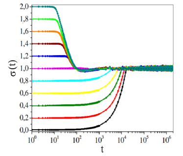
Figure 2: Transient and self-organization for different initial values $\sigma_{0}$ with parameters: $\epsilon=2.0$, $u=0.1$, $A=1.0$, $K=10$, $n=3$ and $N=30000$. The dotted line correspond to the stationary branching ratio $\sigma^{*}$ around which the systems oscillates after a transient: $\sigma^{*}=1.000\pm 0.012$.

The stationary time series for $\sigma(t,N)$ presents fluctuations around an average value $\sigma^{*}(N)$, with standard deviation $\Delta^{*}(N)$. The stationary distribution $P^{*}(\sigma,N)$ is roughly Gaussian (Fig. 3) with the large-$N$ scaling $\sigma^{*}(N)=\sigma_{c}+C_{\sigma}/N$, with the critical point $\sigma_{c}=1$ (see Eq. (11)). The most important result is that it tends to a delta function, with $\Delta^{*}(N)\propto N^{-1/4}$, see inset of Fig. 3.

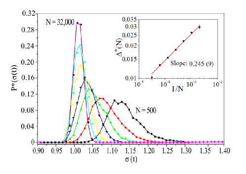
Figure 3: Branching ratio distribution $P^{*}(\sigma)$ for different network sizes. Parameters are: $\epsilon=2.0$, $u=0.1$, $A=0.9$, $K=10$ and $n=3$. Inset: stationary standard deviation $\Delta^{*}$ as a function of $N=500$, $1000$, $2000$, $4000$, $\ldots$, $32000$ (in double logarithmic scale). Symbols are simulations; line is a least-square fit.

In the stationary state, the model is therefore conservative on average, in the sense that it conserves the average number of active sites. In other words, its time-averaged branching ratio $\sigma^{*}(N)$ is critical for large enough $N$.

In Fig. 4 we present theoretical (Eq. (8)) and simulation results for the annealed model. To show the supercritical regime, we used large values for $\epsilon$ given a finite $N$ in order to produce $\rho^{*}(N)>0$. From this figure it is clear that the synaptic dynamics induces the system to lie at the critical point of an absorbing continuous phase transition [7, 8]. This is an important feature, not present in the LHG model, as extensively discussed by Bonachela and Muñoz [16].

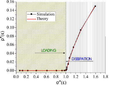
Figure 4: Density of active sites is null for a subcritical system ($\sigma<1$) and grows for the supercritical systems. Theoretical curve (mean field) and simulation points for the annealed model. Arrow to the right indicates the effect of synaptic recovery (mediated by parameters $\epsilon$ and $A$); arrow to the left indicates the effect of synaptic depression, induced by avalanches and mediated by the $u$ parameter. Simulations of supercritical systems are obtained by using large values of $\epsilon$, see Fig. 5. Parameters are: $u=0.1$, $A=0.9$, $K=10$, $n=3$ and $N=10000$.

The main characteristic of our model is that if we plot $\sigma^{*}(N,p)$ versus a parameter $p$ (for example, $\epsilon$, $A$ or $u$), not only $\sigma^{*}(N,p)$ tends to $\sigma_{c}$, but also the parametric derivative $d\sigma^{*}(N,p)/dp$ tends to zero as $N$ increases. This means that a plateau appears around the critical point, so that the parametric dependence (for all parameters) vanishes for large $N$. This can be seen explicitly in the mean field equations, where, for any parameter $p$, we have:

$$\frac{d\sigma^{*}(p)}{dp}\approx C_{p}/N,$$ (13)

for some $p>p_{min}$. For example, the emergence of a parametric plateau for $\epsilon$ can be seen in Fig. 5 (notice the logarithmic scale for $\epsilon$). The same behavior can be observed for parameters $A$ and $u$.

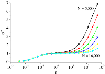
Figure 5: Dependence of the stationary branching ratio $\sigma^{*}$ as a function of $\epsilon$ with $N=500$, $1000$, $2000$, $4000$, $8000$ and $16000$. Symbols are obtained from simulations and lines are mean field results. Parameters as in Fig. 4.

The avalanche finite-size scaling, however, is somewhat problematic, as also observed in other non-conservative models [15, 16]. To obtain a precise scaling of critical avalanches for finite $N$, one needs to tune the parameters. For example, with other parameters fixed, the choice

$$\epsilon=\epsilon_{c}N^{1/3}\>\>\>,$$ (14)

as suggested by Bonachela et al. [15, 16] leads to the correct scaling of the cumulative avalanche size distribution: $C(s)s^{1/2}=f(s/s_{0}(N))$, where $C(s)\equiv\int_{s}^{\infty}P_{size}(s)ds$ and $P_{size}(s)$ is the probability that an avalanche has size $s$ (see Fig. 6).

The scaling with $N$ in Eq. 14 is not so problematic, since it can be absorbed in the original scaling of the synaptic recovery, Eq. 4, that is, by using from start a scaling $\epsilon/KN^{2/3}(A-P_{ij})$. However, critical avalanches are observed only for a definite choice of $\epsilon_{c}(A,u)$ (which now does not depend on $N$). To which extent this tuning implies that our system is a SOqC model is discussed below.

In our model, the cutoff scales as $s_{0}\sim N^{a}$ with $a=3/4$, which is different from the scaling found in the LHG model ($a=1$) [16] or other models ($a=2/3$) [15]. Bonachela et al. [16] observed that a random neighbor version of the LHG model presented an anomalous cutoff exponent, but did not reported its value. Naive scaling considerations, similar to that done in [15], although produce $a=2/3$, do not produce $a=3/4$ nor $a=1$, so we prefer to reserve this issue for future considerations.

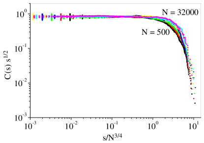
Figure 6: Data collapse of avalanche size ($s$) cumulative distributions $C(s)$ with the scaled parameter $\epsilon_{c}=0.05N^{1/3}$ for different network sizes, with $n=3$, $u=0.1$, $A=1.0$ and $K=10$. The cutoff exponent is $3/4$.

5 Discussion

Bonachela et al. [15, 16] tried to define an universality class, with a definite field theory, for bulk dissipative models that they call Self-Organized quasi-Criticality (SOqC). In doing so, they claimed that this class is characterized by three (necessary) features:

• A) The stationary distribution of couplings values $P^{*}(J)$, which corresponds to $P^{*}(\sigma)$ in our model, has finite variance even in the infinite size limit. The system hoovers around the critical point, with excursions on the supercritical and subcritical phases. The avalanche distribution is constructed by summing supercritical and subcritical avalanches;

• B) The relevant phase transition associated to SOqC is a dynamical percolation transition, not a continuous absorbing phase transition like conservative SOC models [7, 8];

• C) For finite $N$, to obtain a correct scaling with power law avalanches, we must use tuned parameters (like $\epsilon_{c},A_{c},u_{c}$).

The LHG model [18, 16] presents all these features, being classified as a SOqC model. The same occurs with other bulk dissipative models [15]. Our model, however, presents only feature C (see Fig. 6) and lacks the important features A and B. Our model, in contrast to the LHG model, presents vanishing variance for $P^{*}(\sigma)$, so that it does not oscillates nor make supercritical (or subcritical) excursions in the large $N$ limit. Also, the limit $\sigma(N)\rightarrow\sigma_{c}$ is achieved very fast, with weak dependence (tuning) on the parameters $A,\epsilon,u$, because they are constants in front of a $1/N$ factor. Anyway, we observe that, in practice, neuronal networks always work with a very large number of elements (say, one million), compared, for example, with our simulations with $N=32000$. So, the large $N$ limit is the relevant one, and in this limit the avalanche behavior depends very weakly on the parameters, as can be seen from the mean-field results (Eq. 12). So, for large $N$, it is more precise to talk about ”gross-tuning” instead of ”fine-tuning” to describe the finite size avalanche behavior of our model.

Our model lies at the border of a phase transition to an absorbing state (Compact Directed Percolation), instead of a dynamical percolation transition, which is the relevant transition in bona fide SOC models [8, 7, 15]. Since the universality class of our model is different of the LHG model, it should not be put in the same SOqC class. The problem here is of definition: if item C is sufficient to classify a system as SOqC, then our model is SOqC (but them the SOqC will be comprised of two universality classes). But if items A and B are necessary conditions, then our model is not SOqC and another class must be created. What we can claim at this moment is that, since our model lacks features A and B, its behavior resembles much more the conserving SOC models than the LHG model or other non-conservative models [15, 16].

The synaptic depression, mediated by the $u$ parameter, is not conservative. The absence of conserved quantities in the bulk and specially during the (self-organization) transient is another feature that puts our model apart from conventional SOC models. The fact our model violates conservation in the bulk, however, is not an impeditive factor for true criticality. Recently, Moosavi and Montakhab [22] showed that sandpile models with noise (that violates microscopic conservation but preserves average conservation) can be critical if the noiseless model is critical and the noise has zero mean. In the case of our model, the conservation on average is achieved in the stationary state, after a non-conserving transient. So, we conclude that non-conservative bulk dynamics is not a sufficient feature to put a system in the SOqC class.

Which ingredients could account for the differences between our model and the LHG model, which clearly pertain to different universality classes? We identify three main possibilities: i) their model uses continuous-time integrate-and-fire units in contrast to our excitable (SIRS) discrete time units; ii) their units are deterministically coupled via weighted synaptic sums, while our discrete automata are coupled by probabilistic multiplicative synapses; iii) in the LHG model, the avalanches are deterministic and, in our model, they are stochastic; iv) their model is based on a complete graph with $N(N-1)$ synapses, while our model sits on a random graph with finite average degree $K$ and hence $NK$ synapses.

It seems to us that items i), ii), iii) and iv) could hardly be responsible for a change of universality class. On the other hand, item iv) refers to a change of topology, along with a change of time scale in the synaptic dynamics: LHG uses a change of $1/N$ for synapses that already are of order $1/N$ (because of the complete graph topology), which means that synapses are strongly perturbed along the time. In our random neighbor model, since $K=O(1)$, synapses are $O(1)$ and the synaptic change of $1/N$ per time step is infinitesimal for large $N$.

This means that the correction in $P_{ij}$ diminishes for increasing $N$, preventing large excursions or oscillations around the $\sigma^{*}$ point. We believe that this ultra-soft synaptic correction is the missing element, not contemplated in the literature, that produces a SOC model with vanishing variance. If this is true, then one can predict that a simulation of the Levina et al. model with finite $K$ random neighbors should fall in our universality class, that is, presenting vanishing variance for the average coupling in the thermodynamic limit around a CDP transition.

We finally observe that, although $P^{*}(\sigma)$ tends to a delta function, the distribution of local couplings $P^{*}(P_{ij})$ or, equivalently, of local branching ratios $P^{*}(\sigma_{i})$, is not a delta function in the $N\rightarrow\infty$ limit. The two facts are not in contradiction because $\sigma=\frac{1}{N}\sum_{i}^{N}\sigma_{i}$ is an average over $N$ sites and the delta function limit is a large $N$ effect. In other words, the delta function limit is an effect of the law of large numbers for the average $\sigma$ of the $P^{*}(\sigma_{i})$ distribution (which continues to have finite variance for large $N$). This means that the model is nontrivial: there is sufficient diversity in the couplings (synapses) to mimic a real biological network.

In conclusion, we have presented an excitable (SIRS) automata model for neural networks with dynamical synapses which seems to pertain to a new universality class: models with dissipative bulk dynamics that, due to homeostatic mechanisms, achieve a stationary conservative (in average) dynamics. In this model, like in conservative SOC models, the relevant transition pertains to the CPD class. An evolving “control” parameter (the architectural branching ratio) self-organizes to criticality, and its variance around the critical point vanishes in the thermodynamic limit.

References

References

- [1] C. G. Langton. Computation at the edge of chaos: Phase transitions and emergent computation. Physica D, 42:12–37, 1990.
- [2] S. Wolfram. Statistical mechanics of cellular automata. Rev. Mod. Phys., 55:601–644, 1983.
- [3] P Bak, C Tang, and K Wiesenfeld. Self-organized criticality: An explanation of the 1/f noise. Phys. Rev. Lett., 59:381–384, 1987.
- [4] D. R. Chialvo. Emergent complex neural dynamics. Nat. Phys., 6:744–750, 2010.
- [5] S. M. Reia and O. Kinouchi. Conway’s game of LIFE is a near critical metastable state in the multiverse of cellular automata. Phys. Rev. E, 89:052123, 2014.
- [6] H. J. Jensen. Self-Organized Criticality: Emergent Complex Behavior in Physical and Biological Systems. Cambridge University Press, Cambridge, 1998.
- [7] M. A. Muñoz, R. Dickman, A. Vespignani, and S. Zapperi. Avalanche and spreading exponents in systems with absorbing states. Phys. Rev. E, 59(5):6175–6179, 1999.
- [8] R. Dickman, M. A. Muñoz, A. Vespignani, and S. Zapperi. Paths to self-organized criticality. Braz. J. Phys., 30:27 – 41, 2000.
- [9] B. Drossel and F. Schwabl. Self-organized critical forest-fire model. Phys. Rev. Lett., 69(11):1629, 1992.
- [10] J. E. S. Socolar, G. Grinstein, and C. Jayaprakash. On self-organized criticality in nonconserving systems. Phys. Rev. E, 47:2366–2376, Apr 1993.
- [11] H-M. Bröker and P. Grassberger. Random neighbor theory of the olami-feder-christensen earthquake model. Phys. Rev. E, 56:3944–3952, Oct 1997.
- [12] M. L. Chabanol and V. Hakim. Analysis of a dissipative model of self-organized criticality with random neighbors. Phys. Rev. E, 56:R2343–R2346, 1997.
- [13] O. Kinouchi and C. P. C. Prado. Robustness of scale invariance in models with self-organized criticality. Phy. Rev. E, 59(5):4964, 1999.
- [14] J. X. de Carvalho and C. P. C. Prado. Self-organized criticality in the Olami-Feder-Christensen model. Phys. Rev. Lett., 84(17):4006, 2000.
- [15] J. A. Bonachela and M. A. Muñoz. Self-organization without conservation: true or just apparent scale-invariance? J. Stat. Mech., 2009:P09009, 2009.
- [16] J. A. Bonachela, S. de Franciscis, J. J. Torres, and M. A. Muñoz. Self-organization without conservation: are neuronal avalanches generically critical? J. Stat. Mech., 2010:P02015, 2010.
- [17] E. Martin, A. Shreim, and M. Paczuski. Activity-dependent branching ratios in stocks, solar x-ray flux, and the bak-tang-wiesenfeld sandpile model. Phys. Rev. E, 81:016109, Jan 2010.
- [18] A. Levina, J. M. Herrmann, and T. Geisel. Dynamical synapses causing self-organized criticality in neural networks. Nat. Phys., 3:857–860, 2007.
- [19] J. Hesse and T. Gross. Self-organized criticality as a fundamental property of neural systems. Front. Syst. Neurosci., 8:1–5, 2014.
- [20] O. Kinouchi and M. Copelli. Optimal dynamical range of excitable networks at criticality. Nat. Phys., 2:348–351, 2006.
- [21] P. Bak. How Nature Works: The Science of Self-Organized Criticality. Oxford University Press, New York, 1997.
- [22] S. A. Moosavi and A. Montakhab. Mean-field behavior as a result of noisy local dynamics in self-organized criticality: Neuroscience implications. Phys. Rev. E, 89:052139, May 2014.