Helical spin texture of surface states in topological superconductors

Abstract

Surface states of topological noncentrosymmetric superconductors exhibit intricate helical spin textures, i.e., the spin orientation of the surface quasiparticles is coupled to their momentum. Using quasiclassical theory, we study the spin polarization of the surface states as a function of the spin-orbit interaction and superconducting pairing symmetry. We focus on two- and three-dimensional fully gapped and nodal noncentrosymmetric superconductors. For the case of nodal systems, we show that the spin polarization of the topological flat bands is controlled by the spin polarization of the bulk normal states at the bounding gap nodes. We demonstrate that the zero-bias conductance in a magnetic tunnel junction can be used as an experimental test of the surface-state spin polarization.

1 Introduction

Topological superconductors are characterized by protected zero-energy surface states that arise because of the nontrivial topology of the bulk wavefunctions in momentum space [1, 2, 3, 4, 5, 6]. These surface states are associated with one out of several topological invariants. There is currently an intense research effort aimed at identifying topological superconductors, but unambiguous examples of such phases have not yet been established. Noncentrosymmetric superconductors (NCSs), characterized by mixed-parity pairing and strong spin-orbit coupling, have been extensively investigated as possible candidate materials for topological superconductivity [7, 8, 9, 10, 11, 12, 13, 14, 15, 16, 17, 18, 19, 20, 21], the most prominent examples being Li₂Pd_xPt_3-xB [22, 23], BiPd [24, 25, 26], and the heavy-fermion systems CePt₃Si [27] and CeIrSi₃ [28]. Different types of topological surface states in fully gapped and nodal NCSs have recently been classified [10] and their properties have been investigated extensively [9, 10, 11, 12, 29]. It was found that, depending on the crystal point group and the superconducting pairing symmetry, NCSs can exhibit either dispersing Majorana surface states, zero-energy surface flat bands, or arc surface states, as well as edge modes which are not topologically protected. Remarkably, these surface states generally exhibit an intricate helical spin texture. That is, due to spin-orbit interactions, the spin orientation of the quasiparticle surface states is coupled to their momentum [30, 31, 32, 33, 34].

The nontrivial spin texture of NCS surface states is known to have important consequences for the surface physics [8, 14, 30, 31, 32, 33, 34, 35]. For example, the helical character of the spin texture forbids spin-independent scattering between states on opposite sides of the surface Brillouin zone [33], which leaves signatures in Fourier-transformed scanning tunneling spectroscopy [34]. The spin polarization of the edge states also determines their coupling to magnetic exchange fields [8, 14, 32, 33, 35]. Most strikingly, this is responsible for the appearance of a strong interface current in heterostructures involving a nodal NCS and a ferromagnet, which can be used to deduce the existence of nondegenerate zero-energy flat bands in the NCS [32, 33]. Furthermore, the nonzero surface-state spin polarization also gives rise to surface spin currents [30, 31]. Despite the major role played by the helical spin texture of the surface states in the physics of NCSs, it has not yet been systematically studied. In particular, in order to exploit it as a test of the pairing symmetry of NCSs, and hence their topological properties, it is essential to know how the helical spin texture depends on the key variables, namely the spin-orbit coupling and the ratio of singlet to triplet gaps.

In this paper, we use a quasiclassical theory to investigate the spin character of topological surface states in both fully gapped and nodal NCSs and its dependence upon spin-orbit coupling and superconducting pairing symmetry. In particular, in the case of nodal NCSs it is shown that the helical spin texture of the surface states is controlled by the spin polarization of the bulk states at the gap nodes, and thus by the spin structure in the normal state. In our calculation we focus mainly upon two complementary models of two-dimensional NCSs, but we also survey three-dimensional models of direct relevance to experimental systems. In the second part of the paper, we show how the existence of the spin polarization can be evidenced by tunneling into the NCS through a ferromagnetic insulator. Specifically, we show that the zero-bias conductance is very sensitive to the orientation of the barrier magnetization, and also contains signatures of the pairing symmetry.

2 Model Hamiltonian and symmetries

We study subgap states localized at the edge or surface of NCSs described by the Bogoliubov-de Gennes (BdG) Hamiltonian

$$\check{H}({\bf k})=\left(\begin{array}[]{cc}\hat{h}_{0}&\hat{\Delta}\\ \hat{\Delta}^{\dagger}&-(\hat{h}_{0})^{\ast}\end{array}\right).$$ (3)

Here, $\hat{h}_{0}$ describes the normal part of the Hamiltonian,

$$\hat{h}_{0}=\left(\frac{\hbar^{2}}{2m}\,{\bf k}^{2}-\mu\right)\hat{\sigma}^{0}+\lambda\,{\bf l}_{\bf k}\cdot\hat{\boldsymbol{\sigma}},$$ (4)

where $m$ is the effective mass, $\mu$ the chemical potential, $\lambda$ the spin-orbit coupling strength, $\hat{\sigma}^{0}$ the $2\times 2$ unit matrix, $\hat{\bm{\sigma}}$ the vector of Pauli matrices, and ${\bf l}_{\bf k}$ the antisymmetric (i.e., odd in $\mathbf{k}$) spin-orbit coupling pseudovector. The Hamiltonian $\hat{h}_{0}$ in Eq. (4) is diagonalized in the helicity basis, $\hat{h}_{0}=\mbox{diag}(\xi^{+}_{\bf k},\xi^{-}_{\bf k})$, where

$$\xi^{\pm}_{{\bf k}}=\left(\frac{\hbar^{2}}{2m}{\bf k}^{2}-\mu\right)\pm\lambda|{\bf l}_{\bf k}|\,$$ (5)

are the dispersions of the positive ($+$) and negative ($-$) helicity bands.

Due to the breaking of inversion symmetry, the superconducting gap function

$$\hat{\Delta} = \left[\psi_{\bf k}\hat{\sigma}^{0}+{\bf d}_{\bf k}\cdot\hat{\boldsymbol{\sigma}}\right]i\hat{\sigma}^{y}$$ (6)

generically contains both a spin-singlet component $\psi_{\bf k}=\Delta_{s}f(\widetilde{\bf k})=q\Delta_{0}f(\widetilde{\bf k})$ and a spin-triplet component ${\bf d}_{\bf k}=\Delta_{t}f(\widetilde{\bf k})\,{\bf l}_{\widetilde{\bf k}}=(1-q)\Delta_{0}f(\widetilde{\bf k})\,{\bf l}_{\widetilde{\bf k}}$ [36], where $q$ tunes the system from purely triplet ($q=0$) to purely singlet ($q=1$) pairing. We also introduce the dimensionless momentum $\widetilde{\bf k}={\bf k}/k_{F}$, where $k_{F}=(2m\mu)^{1/2}/\hbar$ is the Fermi wavevector in the absence of the spin-orbit coupling. The orientation of the vector $\mathbf{d}_{\mathbf{k}}$ parallel to ${\bf l}_{\bf k}$ implies pairing only between states on the same helicity Fermi surface, opening the gaps

$$\Delta^{\pm}_{\bf k}=\big{[}q\pm(1-q)|{\bf l}_{\widetilde{\bf k}}|\big{]}\,\Delta_{0}f(\widetilde{\bf k}).$$ (7)

The form factor $f({\bf k})$ determines the orbital-angular-momentum pairing state. In the following we focus on two cases: $f({\bf k})=1$ for a NCS with ($s+p$)-wave pairing symmetry [15, 18, 29, 30, 31] and $f({\bf k})=2k_{x}k_{y}$ for a ($d_{xy}+p$)-wave pairing state [12, 33].

The momentum dependence of the spin-orbit pseudovector ${\bf l}_{\bf k}$ is restricted by the symmetries of the noncentrosymmetric crystal. We consider three different crystallographic point groups: tetragonal $C_{4v}$, cubic $O$, and monoclinic $C_{2}$. Within a small-momentum expansion around the $\Gamma$ point [37], the vector $\mathbf{l}_{\mathbf{k}}$ for the tetragonal point group $C_{4v}$ is written as

$$\qquad{\bf l}_{\bf k}=\hat{\bf x}\,k_{y}-\hat{\bf y}\,k_{x}.$$ (8)

Examples of $C_{4v}$ NCSs are CePt₃Si [27] and CeIrSi₃ [28]. This form of $\mathbf{l}_{\mathbf{k}}$ is often referred to as Rashba spin-orbit coupling. For the cubic point group $O$ we have

$$\qquad{\bf l}_{\bf k}=\hat{\bf x}\,k_{x}(1+g_{2}[k_{y}^{2}+k_{z}^{2}])+\hat{\bf y}\,k_{y}(1+g_{2}[k_{x}^{2}+k_{z}^{2}])+\hat{\bf z}\,k_{z}(1+g_{2}[k_{x}^{2}+k_{y}^{2}]),$$ (9)

where we include the second-order spin-orbit coupling $g_{2}$. This point group is relevant for Li₂Pd_xPt_3-xB [22, 23] and Mo₃Al₂C [38, 39]. For the monoclinic group $C_{2}$, which is relevant for BiPd [24, 25, 26], we have

$$\qquad{\bf l}_{\bf k}=\hat{\bf x}\,(a_{1}k_{x}+a_{2}k_{y})+\hat{\bf y}\,(a_{3}k_{x}+a_{4}k_{y})+\hat{\bf z}\,a_{5}k_{z}.$$ (10)

A three-dimensional $C_{2}$ NCS with $\mathbf{l}_{\mathbf{k}}$ given by Eq. (10) generically exhibits nodal rings in the BdG spectrum. The number of these nodal rings and their position in the Brillouin zone depend on the particular values of the parameters $a_{i}$ and the singlet-triplet ratio $q$. For the numerical calculations, we set $a_{i}=1$ for all $i=1,\ldots,5$. Other parameter choices give qualitatively similar results.

The BdG Hamiltonian $\check{H}({\bf k})$ possesses all three symmetries which form the basis of the topological ten-fold way classification [1, 2, 3]: time-reversal, particle-hole, and chiral symmetry. Time-reversal acts as $\check{U}_{T}^{{\dagger}}\check{H}({\bf k})\check{U}_{T}=\check{H}^{\!\mathrm{T}}(-{\bf k})$, where $\check{U}_{T}=\tau^{0}\otimes i\sigma^{y}$ and $\tau^{i}$ are the Pauli matrices in Nambu space. The time-reversal operator squares to $\check{U}_{T}\check{U}_{T}^{\ast}=(\tau^{0}\otimes i\sigma^{y})(\tau^{0}\otimes i\sigma^{y})=\tau^{0}\otimes(-\sigma^{0})=-\mathbbm{1}$, where $\mathbbm{1}$ is the $4\times 4$ unit matrix. Particle-hole symmetry acts on $\check{H}({\bf k})$ as $\check{U}_{C}^{{\dagger}}\check{H}({\bf k})\check{U}_{C}=-\check{H}^{\!\mathrm{T}}(-{\bf k})$, where $\check{U}_{C}=\tau^{x}\otimes\sigma^{0}$. The particle-hole-conjugation operator squares to $\check{U}_{C}\check{U}_{C}^{\ast}=(\tau^{x}\otimes\sigma^{0})(\tau^{x}\otimes\sigma^{0})=\tau^{0}\otimes\sigma^{0}=+\mathbbm{1}$. Hence, $\check{H}({\bf k})$ belongs to symmetry class DIII. Combining time-reversal and particle-hole symmetry yields the so-called chiral symmetry, which acts on the BdG Hamiltonian as $\check{U}_{S}\check{H}({\bf k})+\check{H}({\bf k})\check{U}_{S}=0$, where $\check{U}_{S}=i\check{U}_{T}\check{U}_{C}=-\tau^{x}\otimes\sigma^{y}$.

2.1 Surface states

In order to obtain the surface-state wavefunctions we solve the BdG equations

$$\left(\begin{array}[]{cc}\hat{h}_{0}&\hat{\Delta}\\ \hat{\Delta}^{\dagger}&-(\hat{h}_{0})^{\ast}\end{array}\right)\Psi({\bf r})=E\Psi({\bf r})$$ (11)

subject to the boundary conditions $\left.\Psi({\bf r})\right|_{r_{\perp}=0}=0$ and $\left.\Psi({\bf r})\right|_{r_{\perp}\to+\infty}=0$, where $r_{\perp}$ is the coordinate normal to the surface. The wavevector component ${\bf k}_{\parallel}$ parallel to the surface is a good quantum number by translational invariance, and so we henceforth work with the Fourier-transformed wavefunction $\Psi({\bf k}_{\parallel};r_{\perp})$, which is an eigenfunction of the one-dimensional Hamiltonian $\check{H}({\bf k}_{\parallel})$. Depending on the value of ${\bf k}_{\parallel}$, we distinguish two cases when constructing the wavefunction ansatz: the surface momentum lies within both projected Fermi surfaces or only within the projected (larger) negative-helicity Fermi surface.

2.1.1 Surface momentum within projection of both Fermi surfaces.

In this case there are wavevectors on both positive and negative helicity Fermi surfaces which project onto the surface momentum ${\bf k}_{\parallel}$, specifically ${\bf k}_{\pm}=({\bf k}_{\parallel},k_{\perp,\pm})$ and ${\bf k}^{\prime}_{\pm}=({\bf k}_{\parallel},{k}^{\prime}_{\perp,\pm})$, where the perpendicular wavevector components $k_{\perp,\pm}$ and ${k}^{\prime}_{\perp,\pm}$ have opposite sign. The wavefunction ansatz for the bound state is then a superposition of evanescent states in the various channels,

$$\Psi({\bf k}_{\parallel};r_{\perp}) = \sum_{\nu=\pm}\sum_{{\bf k}={\bf k}_{\nu},{\bf k}^{\prime}_{\nu}}\,\alpha_{\nu}({\bf k})\psi_{\nu}({\bf k})\,e^{ik_{\perp}r_{\perp}}e^{-\kappa^{\nu}_{{\bf k}}r_{\perp}},$$ (12)

where the spinors in Eq. (12) are given by

$$\psi_{\pm}({\bf k})=\left(\begin{array}[]{cccc}1,&\pm\frac{l^{x}_{\bf k}+il^{y}_{\bf k}}{|{\bf l}_{\bf k}|\pm l^{z}_{\bf k}},&\mp\frac{l^{x}_{\bf k}+il^{y}_{\bf k}}{|{\bf l}_{\bf k}|\pm l^{z}_{\bf k}}\,\gamma^{\pm}_{\bf k},&\gamma^{\pm}_{\bf k}\end{array}\right)^{\mathrm{T}},$$ (13)

with

$$\gamma^{\pm}_{\bf k} = \frac{1}{\Delta^{\pm}_{\bf k}}\left[E-i\mathop{\textrm{sgn}}(v^{\pm}_{F,\perp}({\bf k}))\sqrt{|\Delta^{\pm}_{\bf k}|^{2}-E^{2}}\right],$$ (14)

$$\kappa^{\pm}_{\bf k} = \frac{1}{\hbar\,|v^{\pm}_{F,\perp}({\bf k})|}\sqrt{|\Delta^{\pm}_{\bf k}|^{2}-E^{2}},$$ (15)

and $v^{\pm}_{F,\perp}({\bf k})$ is the component of the Fermi velocity normal to the surface. A bound state is realized when it is possible to choose nonzero coefficients $\alpha_{\nu}({\bf k})$ in Eq. (12) such that the wavefunction obeys the normalization condition

$$1=\int^{\infty}_{0}dr_{\perp}\Psi^{\dagger}({\bf k}_{\parallel};r_{\perp})\,\Psi({\bf k}_{\parallel};r_{\perp})$$ (16)

and vanishes at the surface. The former condition is satisfied if $|E|<\min\{|\Delta^{\pm}_{{\bf k}_{\pm}}|,|\Delta^{\pm}_{{\bf k}^{\prime}_{\pm}}|\}$. From Eq. (12) we see that the latter condition is equivalent to

$$\det\left[\begin{array}[]{cccc}\psi_{+}({\bf k}_{+})&\psi_{+}({\bf k}^{\prime}_{+})&\psi_{-}({\bf k}_{-})&\psi_{-}({\bf k}^{\prime}_{-})\end{array}\right]=0.$$ (17)

Solutions of this equation satisfying $|E|<\min\{|\Delta^{\pm}_{{\bf k}_{\pm}}|,|\Delta^{\pm}_{{\bf k}^{\prime}_{\pm}}|\}$ are the bound-state energies, which can belong to either dispersing or zero-energy flat bands.

2.1.2 Surface momentum only within projection of negative-helicity Fermi surface.

In the case that there are propagating solutions only on the negative-helicity Fermi surface, the positive-helicity components of the wavefunction ansatz in Eq. (12) are replaced by

$$\big{[}\alpha_{e,+}({\bf p})\phi_{e}({\bf p})+\alpha_{h,+}({\bf p})\phi_{h}({\bf p})\big{]}\,e^{ip_{\perp}r_{\perp}},$$ (18)

where ${\bf p}=({\bf k}_{\parallel},p_{\perp})$ satisfies $\xi^{+}_{\bf p}=0$ and the imaginary part of $p_{\perp}$ is positive. The spinors $\phi_{e}({\bf p})$ and $\phi_{h}({\bf p})$ describe an electronlike or holelike state in the absence of the pairing potential,

$$\phi_{e}({\bf p}) = \left(\begin{array}[]{cccc}1,&\frac{l^{x}_{\bf p}+il^{y}_{\bf p}}{|{\bf l}_{\bf p}|+l^{z}_{\bf p}},&0,&0\end{array}\right)^{\!\mathrm{T}},$$ (20)

$$\phi_{h}({\bf p}) = \left(\begin{array}[]{cccc}0,&0,&-\frac{l^{x}_{\bf p}+il^{y}_{\bf p}}{|{\bf l}_{\bf p}|+l^{z}_{\bf p}},&1\end{array}\right)^{\!\mathrm{T}}.$$ (22)

The condition for the existence of the bound state now becomes

$$\det\left[\begin{array}[]{cccc}\phi_{e}({\bf p})&\phi_{h}({\bf p})&\psi_{-}({\bf k}_{-})&\psi_{-}({\bf k}^{\prime}_{-})\end{array}\right]=0.$$ (23)

Unlike Eq. (17), this only allows for the existence of nondegenerate zero-energy flat bands, which occur whenever $\mathop{\textrm{sgn}}(\Delta^{-}_{{\bf k}_{-}})=-\mathop{\textrm{sgn}}(\Delta^{-}_{{\bf k}^{\prime}_{-}})$.

2.1.3 Symmetries of the wavefunctions.

The symmetries characterizing the bulk BdG Hamiltonian remain valid for the edge states. Hence, for every surface-state wavefunction $\Psi({\bf k}_{\parallel};r_{\perp})$ satisfying $\check{H}({\bf k}_{\parallel})\Psi({\bf k}_{\parallel};r_{\perp})=E({\bf k}_{\parallel})\Psi({\bf k}_{\parallel};r_{\perp})$, there is a time-reversed partner $\check{U}_{T}\Psi^{\ast}({\bf k}_{\parallel};r_{\perp})$, which is an eigenfunction of $\check{H}(-{\bf k}_{\parallel})$ with the same energy $E(-{\bf k}_{\parallel})=E({\bf k}_{\parallel})$, i.e.,

$$\check{H}(-{\bf k}_{\parallel})\check{U}_{T}\Psi^{\ast}({\bf k}_{\parallel};r_{\perp})=E({\bf k}_{\parallel})\check{U}_{T}\Psi^{\ast}({\bf k}_{\parallel};r_{\perp}).$$ (24)

Due to Kramer’s theorem, $\Psi({\bf k}_{\parallel};r_{\perp})$ and $\check{U}_{T}\Psi^{\ast}({\bf k}_{\parallel};r_{\perp})$ are orthogonal for all ${\bf k_{\parallel}}$. Similarly, particle-hole symmetry dictates that for every surface-state eigenfunction $\Psi({\bf k}_{\parallel};r_{\perp})$ there is a particle-hole-reversed partner $\check{U}_{C}\Psi^{\ast}({\bf k}_{\parallel};r_{\perp})$, which is an eigenfunction of $\check{H}(-{\bf k}_{\parallel})$ with energy $-E({\bf k}_{\parallel})$, i.e.,

$$\check{H}(-{\bf k}_{\parallel})\check{U}_{C}\Psi^{\ast}({\bf k}_{\parallel};r_{\perp})=-E({\bf k}_{\parallel})\check{U}_{C}\Psi^{\ast}({\bf k}_{\parallel};r_{\perp}).$$ (25)

Finally, the presence of chiral symmetry requires that for every surface state $\Psi({\bf k}_{\parallel};r_{\perp})$ with energy $E({\bf k}_{\parallel})$ there is a chiral-symmetric partner $\check{U}_{S}\Psi({\bf k}_{\parallel};r_{\perp})$ with energy $-E({\bf k}_{\parallel})$, i.e.,

$$\check{H}({\bf k}_{\parallel})\check{U}_{S}\Psi({\bf k}_{\parallel};r_{\perp})=-E({\bf k}_{\parallel})\check{U}_{S}\Psi({\bf k}_{\parallel};r_{\perp}).$$ (26)

We observe that all eigenfunctions of $\check{H}({\bf k}_{\parallel})$ can be chosen to be simultaneous eigenfunctions of $\check{U}_{S}$ with chirality eigenvalue $\pm 1$ [19].

2.2 Spin polarization

We define the $\mu$-component of the spin polarization of the surface state with energy $E$ and surface momentum ${\bf k}_{\parallel}$ as the expectation value

$$\rho^{\mu}_{\mathrm{tot}}(E,{\bf k}_{\parallel})=\int_{0}^{\infty}dr_{\perp}\Psi^{\dagger}({\bf k}_{\parallel};r_{\perp})\check{S}^{\mu}\Psi({\bf k}_{\parallel};r_{\perp})$$ (27)

of the total spin operator $\check{S}^{\mu}$ with respect to the wavefunction $\Psi({\bf k}_{\parallel};r_{\perp})$. The total spin operator in Nambu space reads

$$\check{S}^{\mu}=\left(\begin{array}[]{c c}\sigma^{\mu}&0\cr 0&-\left[\sigma^{\mu}\right]^{\ast}\cr\end{array}\right),$$ (28)

with $\mu=x,y,z$. Note that the coupling of the surface states to an external exchange field is determined by the total spin polarization [32, 33]. On the other hand, the surface spin current of NCSs can be understood in terms of the spin polarization of the electronlike (or holelike) part of the surface-state wavefunction $\Psi({\bf k}_{\parallel};r_{\perp})$ [31, 30]. Hence, it is useful to define an electronlike (holelike) spin polarization

$$\rho^{\mu}_{\mathrm{e(h)}}(E,{\bf k}_{\parallel})=\int_{0}^{\infty}dr_{\perp}\Psi^{\dagger}({\bf k}_{\parallel};r_{\perp})\check{S}^{\mu}_{e(h)}\Psi({\bf k}_{\parallel};r_{\perp})$$ (29)

in terms of the electronlike and holelike spin operators

$$\check{S}^{\mu}_{\mathrm{e}}=\left(\begin{array}[]{cc}\sigma^{\mu}&0\cr 0&0\cr\end{array}\right),\qquad\check{S}^{\mu}_{\mathrm{h}}=\left(\begin{array}[]{cc}0&0\cr 0&-\left[\sigma^{\mu}\right]^{\ast}\cr\end{array}\right),$$ (30)

respectively.

The symmetry properties of the edge-state wavefunctions are reflected in their spin polarization. Specifically, the various symmetries give the following constraints:

• time-reversal symmetry:

  $$\quad\rho^{\mu}_{\mathrm{e(h)}}(E,{\bf k}_{\parallel})=-\rho^{\mu}_{\mathrm{e(h)}}(E,-{\bf k}_{\parallel}),\quad\rho^{\mu}_{\mathrm{tot}}(E,{\bf k}_{\parallel})=-\rho^{\mu}_{\mathrm{tot}}(E,-{\bf k}_{\parallel}),$$ (31)

• particle-hole symmetry:

  $$\quad\rho^{\mu}_{\mathrm{e(h)}}(E,{\bf k}_{\parallel})=-\rho^{\mu}_{\mathrm{h(e)}}(-E,-{\bf k}_{\parallel}),\quad\rho^{\mu}_{\mathrm{tot}}(E,{\bf k}_{\parallel})=-\rho^{\mu}_{\mathrm{tot}}(-E,-{\bf k}_{\parallel}),$$ (32)

• chiral symmetry:

  $$\quad\rho^{\mu}_{\mathrm{\mathrm{e(h)}}}(E,{\bf k}_{\parallel})=\rho^{\mu}_{\mathrm{h(e)}}(-E,{\bf k}_{\parallel}),\quad\rho^{\mu}_{\mathrm{tot}}(E,{\bf k}_{\parallel})=\rho^{\mu}_{\mathrm{tot}}(-E,{\bf k}_{\parallel}).$$ (33)

Due to the chiral and particle-hole symmetries, it is only necessary to consider the total spin polarization for the bound states with nonnegative energies. Time-reversal symmetry requires that the spin polarization is an odd function of the surface momentum, and so there will be no spin accumulation at the surface, although a surface spin current is permitted [30, 31].

In the following we present results only for the total spin polarization and we thus drop the subscript “tot”. To evaluate the spin polarization, it is necessary to determine the coefficients $\alpha_{\nu}({\bf k})$ in the wavefunctions. This is equivalent to determining the null space of the matrices with column vectors given by the spinors in the wavefunction ansatz. In general it is necessary to numerically calculate the coefficients and the spin polarization. In our numerical calculations we take the BCS correlation length $\xi_{0}=2\hbar v_{F}/\pi\Delta_{0}=100\,k_{F}^{-1}$ where $v_{F}=\hbar k_{F}/m$; although this is at the lower limit of physical values, larger values only result in minor quantitative changes. We also introduce the dimensionless spin-orbit coupling $\widetilde{\lambda}=\lambda m/\hbar^{2}k_{F}$. Due to the symmetries of the spin polarization, we restrict ourselves to nonnegative bound-state energies and henceforth drop the energy argument in the spin polarization, $\rho^{\mu}(E,{\bf k}_{\parallel})\rightarrow\rho^{\mu}({\bf k}_{\parallel})$.

3 Edge states of two-dimensional NCSs

We commence by considering the $(10)$ edge states of two-dimensional NCSs with $C_{4v}$ point group, which can be obtained by restricting the three-dimensional model to the $k_{z}=0$ plane. The normal-state Fermi surface consists of two concentric circles with radii $k_{F,\pm}=k_{F}\,[(1+\widetilde{\lambda}^{2})^{1/2}\mp\widetilde{\lambda}]$. The two choices for the superconducting form factor $f({\bf k})$, cf. Eq. (7), give qualitatively different topologies and thus very different edge states. The system is fully gapped in the ($s+p$)-wave case for all values of the singlet-triplet parameter $q$, except at $q=q_{c}=k_{F,-}/(k_{F}+k_{F,-})$ where the negative-helicity gap vanishes. This marks the boundary between the topologically nontrivial ($q<q_{c}$) and trivial ($q>q_{c}$) regimes, and the topology is characterized by a $\mathbb{Z}_{2}$ bulk topological invariant. In agreement with the bulk-boundary correspondence, helical edge states with Majorana zero-energy modes are present only in the topological state. In contrast, a bulk topological invariant cannot be defined for the nodal ($d_{xy}+p$)-wave NCS. Nevertheless, this system possesses topologically protected flat-band zero-energy edge states. The topological protection arises by interpreting the edge state at edge momentum $k_{y}$ to be the edge state of a one-dimensional Hamiltonian $\check{H}(k_{y})$ which falls into class AIII. The topology of this Hamiltonian is characterized by a $\mathbb{Z}$ number; in particular, when this number evaluates to $\pm 1$, the edge states are nondegenerate, i.e., they have a Majorana character [8, 9, 10, 11, 12, 13].

3.1 ($s+p$)-wave NCS

In figure 1 we plot the dispersion and the spin polarization $\rho^{\mu}(k_{y})$ of the edge states with nonnegative energy in the ($s+p$)-wave phase. As can be seen from panels (a) and (d), the helical edge states are only present in the topologically nontrivial regime ($q<q_{c}$) and within the projection of the positive-helicity Fermi surface ($|k_{y}|\leq k_{F,+}$). The remaining panels of figure 1 reveal that the edge states exhibit a spin polarization in the $xz$ plane, with a particularly strong component along the $x$ axis. The spin polarization depends upon the singlet-triplet parameter $q$ and the spin-orbit coupling strength $\widetilde{\lambda}$, and changes sign as these quantities are increased. Note that the spin polarization is not determined by the topological properties of the system alone: in the topologically nontrivial state it is possible to continuously deform the system to a helical $p$-wave superconductor without spin-orbit coupling (i.e., $\Delta_{s}=0$ and $\widetilde{\lambda}=0$), for which the edge states have vanishing spin polarization.

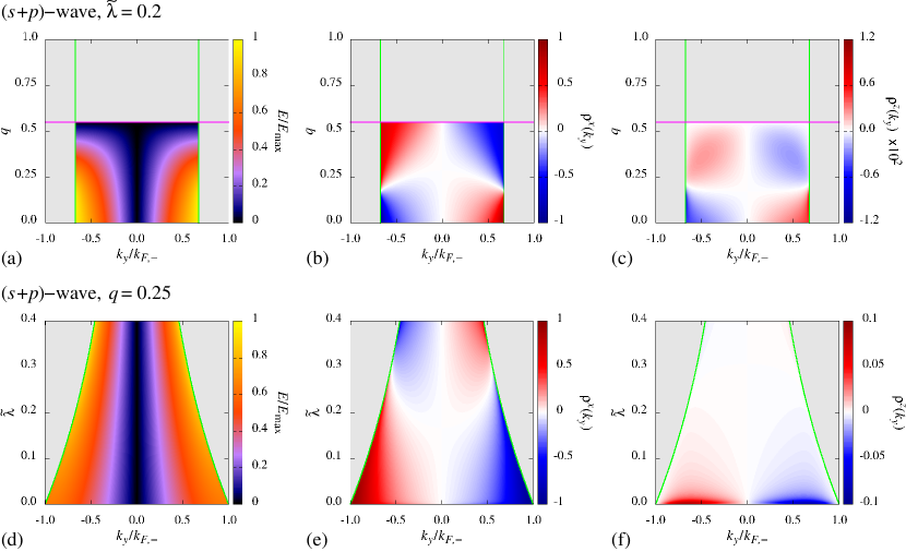
Figure 1: Evolution of the momentum-resolved edge-state spectrum and spin polarization at the $(10)$ edge of the 2D $C_{4v}$ ($s$+$p$)-wave NCS (a)–(c) as a function of the singlet-triplet parameter $q$ and (d)–(f) as a function of the spin-orbit strength $\widetilde{\lambda}$. The first column gives the dispersion of the nonnegative-energy edge states compared to the maximum energy in the plot, $E_{\rm{max}}$, while the second and third columns give the total $x$- and $z$-spin polarization, respectively. The $y$-spin polarization vanishes. Grey regions indicate the absence of any edge state. The green lines indicate the projected edge of the positive-helicity Fermi surface, while the horizontal magenta line in panels (a)–(c) indicates the negative-helicity gap closing at $q=q_{c}$.

The dramatic variation of the spin polarization is controlled by the spin-orbit coupling and the gap structure. Focusing upon the $x$-spin polarization, we gain insight into their interplay by first considering the polarization close to $|k_{y}|=k_{F,+}$, where the subgap states enter the continuum at energy $E=\min\{\Delta^{+}_{\bf k},|\Delta^{-}_{\bf k}|\}$. As $|k_{y}|$ approaches $k_{F,+}$, the edge states smoothly evolve to match the bulk wavefunctions at the edge of the continuum. The $x$-spin polarization of the edge state will hence also evolve to match that of the continuum states with transverse momentum $k_{y}$, which for the $\nu=\pm$ helicity band is given by $\nu k_{y}/k_{F,\nu}$. Thus, when the negative-helicity gap is the smallest (i.e., for $q>\widetilde{\lambda}/(1+{\widetilde{\lambda}})$), the edge states close to the gap edge are dominated by the negative-helicity components, and hence have spin polarization $-\mathop{\textrm{sgn}}(k_{y})\,k_{F,+}/k_{F,-}$. On the other hand, the edge states close to the continuum have spin polarization $\mathop{\textrm{sgn}}(k_{y})$ when the positive-helicity gap is the smallest (i.e., for $q<\widetilde{\lambda}/(1+{\widetilde{\lambda}})$). This is in excellent agreement with the numerical results. This argument also holds away from the gap edges: the full results for the $x$-spin polarization is well represented by

$$\rho^{x}(k_{y})\approx\sum_{\nu=\pm}\nu\,\frac{k_{y}}{k_{F,\nu}}\int^{\infty}_{0}dx\,[{\cal P}_{\nu}\Psi(k_{y};x)]^{\dagger}\,{\cal P}_{\nu}\Psi(k_{y};x),$$ (34)

where ${\cal P}_{\nu}$ projects onto the $\nu$ helicity components in Eq. (12). That is, the variation of the $x$-spin polarization reflects the relative strength of the positive- and negative-helicity components of the wavefunction.

Such an argument cannot be made for the $z$-spin polarization, however, as the bulk states of the two-dimensional NCS are polarized in the $xy$ plane. This also holds for the spinors in Eq. (13) comprising the wavefunction, i.e., $\psi^{\dagger}_{\pm}({\bf k})\check{S}^{z}\psi_{\pm}({\bf k})=0$. The $z$-spin polarization thus arises entirely due to the interference between the different channels in the wavefunction ansatz in Eq. (12); this is in contrast to the $x$-spin polarization, where $\psi^{\dagger}_{\pm}({\bf k})\check{S}^{x}\psi_{\pm}({\bf k})$ is generally nonzero. As such, the spin density

$$\rho^{\mu}(k_{y},x)=\Psi^{\dagger}(k_{y};x)\check{S}^{\mu}\Psi(k_{y};x)$$ (35)

shows damped oscillations about zero for $\mu=z$, whereas for $\mu=x$ it oscillates about a finite value. It hence follows that the integrated $z$-spin density will be much smaller than that for the $x$-spin density, in agreement with the numerics. For illustration, we plot in figures 2(a) and (b) typical examples of the $x$- and $z$-spin densities, respectively.

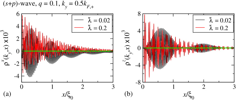
Figure 2: Typical plots of the spin density $\rho^{\mu}(k_{y},x)$ of an edge state of the ($s+p$)-wave NCS for (a) $\mu=x$ and (b) $\mu=z$. We take $q=0.1$ and $k_{y}=0.5\,k_{F,+}$. The green line indicates zero.

3.2 ($d_{xy}+p$)-wave NCS

The dispersion and the spin polarization of the edge states with nonnegative energy in the ($d_{xy}+p$)-wave NCS are shown in figure 3. Zero-energy flat bands are clearly present for $k_{F,+}<|k_{y}|<k_{F,-}$ at all values of the singlet-triplet parameter $q$, and also at $|k_{y}|<k_{F,+}$ for $q>q_{c}$. Whereas the former are nondegenerate, the latter are doubly degenerate, similar to the flat bands at the edge of a $d_{xy}$-wave superconductor without spin-orbit coupling. Dispersing states are present at $|k_{y}|<k_{F,+}$ for $q<q_{c}$ and sufficiently small spin-orbit coupling. Similarly to the ($s+p$)-wave NCS, the edge states are spin-polarized in the $xz$ plane, with the $z$-spin polarization generally much weaker than the $x$-spin polarization. Note that the spin polarization of the doubly degenerate zero-energy flat bands is the sum of the polarizations of the corresponding two states.

The spin polarization of the dispersing edge states can be understood by the same arguments as above. More interesting is the spin polarization of the topologically nontrivial nondegenerate zero-energy flat bands at $k_{F,+}<|k_{y}|<k_{F,-}$, in particular their $x$-spin polarization: as can be seen in figures 3(b) and (e), this component shows no dependence upon the singlet-triplet parameter $q$ or the spin-orbit coupling $\widetilde{\lambda}$. Furthermore, there appears to be a discontinuity in the spin polarization across the projected nodal points of the positive-helicity gap at $k_{y}=\pm k_{F,+}$.

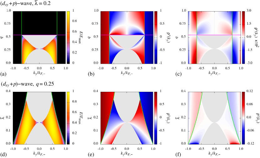
Figure 3: Evolution of the momentum-resolved edge-state spectrum and spin polarization for the 2D $C_{4v}$ ($d_{xy}$+$p$)-wave NCS (a)–(c) as a function of the singlet-triplet parameter $q$ and (d)–(f) as a function of the spin-orbit strength $\widetilde{\lambda}$. The first column gives the dispersion of the nonnegative-energy edge states, while the second and third columns give the total $x$- and $z$-spin polarization, respectively. The $y$-spin polarization vanishes. Grey regions indicate the absence of any edge state. Black regions in panels (a), (d) denote flat zero-energy bands. The green lines indicate the projected edge of the positive-helicity Fermi surface, while the horizontal magenta line in panels (a)–(c) indicates the negative-helicity gap closing at $q=q_{c}$.

It is possible to obtain analytic expressions for the wavefunctions of the nondegenerate flat-band states [12, 40], which read

$$\Psi(k_{y};x)=N\left\{\left[A_{k_{y}}\left(e^{ip_{+}x}-e^{-\kappa_{-}x}\cos(k_{x,-}x)\right)-\frac{k_{F,-}+A_{k_{y}}k_{y}}{k_{x,-}}\,e^{-\kappa_{-}x}\sin(k_{x,-}x)\right]\right.$$

$$\times\left(\begin{array}[]{cccc}i\mathop{\textrm{sgn}}(k_{y}[q-(1-q)k_{F,-}])\,,&0\,,&0\,,&1\end{array}\right)^{\!\mathrm{T}}$$ (37)

$$+\left[\left(e^{ip_{+}x}-e^{-\kappa_{-}x}\cos(k_{x,-}x)\right)+\frac{A_{k_{y}}k_{F,-}+k_{y}}{k_{x,-}}\,e^{-\kappa_{-}x}\sin(k_{x,-}x)\right]$$

$$\left.\times\left(\begin{array}[]{cccc}0\,,&i\mathop{\textrm{sgn}}(k_{y}[q-(1-q)k_{F,-}])\,,&-1\,,&0\end{array}\right)^{\!\mathrm{T}}\right\},$$ (39)

where $A_{k_{y}}=(k_{y}-p_{+})/k_{F,+}$, $p_{+}=i(k_{y}^{2}-k_{F,+}^{2})^{1/2}$, $k_{x,-}=(k_{F,-}^{2}-k_{y}^{2})^{1/2}$, $N$ is a normalization constant,

$$\kappa_{-}=\frac{4}{\hbar v_{F}}\frac{1+\frac{k_{F,-}}{k_{F}}}{1+\frac{k_{F,+}}{k_{F,-}}}|q-q_{c}|\Delta_{0}\frac{k_{y}}{k_{F}},$$ (40)

and the other quantities are as defined in section 2. From the wavefunction Eq. (39) it is possible to explicitly calculate the spin polarization. For the $x$-spin polarization, the unwieldy full expression is greatly simplified in the limit $\kappa_{-}\ll k_{x,-},\,|p_{+}|$, which is realized for $|k_{y}|$ close to $k_{F,-}$, where we find

$$\rho^{x}(k_{y})\cong-\frac{k_{y}}{k_{F,-}},$$ (41)

in excellent agreement with the numerics. Note that this is the $x$-spin polarization expected for purely negative-helicity states; indeed, negative-helicity states contribute almost all the weight of the flat-band wavefunctions for $\kappa_{-}\ll|p_{+}|$, as the positive-helicity components are sharply localized at the edge. Significant deviations from Eq. (41) therefore occur when the localization length for the negative-helicity sector is comparable or larger than that for positive helicity, i.e., for $\kappa_{-}\gtrsim|p_{+}|$, which occurs close to the projected positive-helicity gap nodes at $k_{y}=\pm k_{F,+}$. This is not surprising, as the edge-state wavefunction must evolve to match the bulk positive-helicity wavefunctions at the node. Thus, within the momentum range $|k_{y}|/k_{F,+}-1\lesssim([q-q_{c}]/\xi_{0}k_{F})^{2}$ (obscured by the green lines in figure 3), the $x$-spin polarization reverses and at $|k_{y}|=k_{F,+}+0^{+}$ is equal to $\mathop{\textrm{sgn}}(k_{y})$. This illustrates an important principle: the spin polarization of the nondegenerate flat bands varies so that it matches the spin polarization of the bulk positive-helicity states at the bounding nodes. Since the positive-helicity gap vanishes here, these are in fact identical to the positive-helicity states in the normal phase.

4 Surface states of three-dimensional NCSs

We now turn to the case of three-dimensional NCSs. For simplicity we ignore the spin-orbit splitting of the Fermi surfaces, i.e., we set $\widetilde{\lambda}=0$. The effects of the inversion-symmetry breaking is therefore restricted to the mixed parity of the superconducting gap. We do not expect this to qualitatively alter our results [10]. Assuming the $s$-wave form-factor $f({\bf k})=1$, nodal rings appear only in the negative-helicity gap for $0<q<q_{c}=0.5$; for $q>q_{c}$ the system is fully gapped and topologically trivial. Nondegenerate zero-energy flat-band surface states appear in the surface Brillouin zone for ${\bf k}_{\parallel}$ lying within the projections of the nodal lines, such that the negative-helicity gap has opposite sign at ${\bf k}_{-}$ and ${\bf k}^{\prime}_{-}$, i.e., on opposite sides of the Fermi surface [9, 10, 11].

In figure 4 we plot typical dispersions of surface states for the three point groups considered here: monoclinic $C_{2}$ in the left column, tetragonal $C_{4v}$ in the middle column, and cubic $O$ in the right column. In each case the zero-energy flat-band states coexist with dispersing edge states. Similar to the two-dimensional systems studied above, both the dispersing and the flat-band states are generally spin polarized, as shown in the lower three rows of figure 4. Note that the spin polarization is given with respect to the crystal axes.

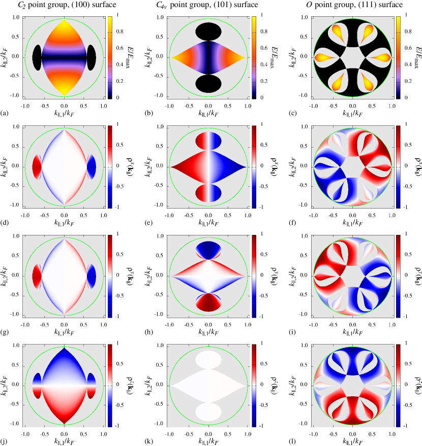
Figure 4: Edge-state dispersion and spin polarization of 3D NCS systems. Each column shows results for a different point group symmetry: from the left we have the (100) surface of a $C_{2}$ NCS, the (101) surface of a $C_{4v}$ NCS, and the (111) surface of an $O$ NCS. The first row gives the dispersion of the nonnegative-energy edge states, while the second, third, and fourth rows shows the spin polarization along the $x$, $y$, and $z$ axis of the crystal, respectively. In all panels we take $q=0.25$ and assume negligible spin-orbit splitting, $\widetilde{\lambda}=0$. Grey indicates the absence of any surface state, black regions in panels (a), (b), (c) denote flat zero-energy bands, and the green circle is the projection of the Fermi surface.

Although the variation of the spin polarization across the flat band can be rather complicated, we know from the discussion of the two-dimensional systems that the polarization of the flat-band edge states must match that of the normal bulk states at the bounding nodes. Since the gap nodes appear only in the negative-helicity sector, the spin polarization close to the edge of the flat bands is $-{\bf l}_{\bf k}/|{\bf l}_{\bf k}|$ where ${\bf k}$ lies on the gap node. This is nicely illustrated by the case of the $C_{4v}$ NCS, where the spin polarization of the flat-band states rotates in a clockwise direction in the $xy$ plane as one moves around their edge in the same sense, consistent with the negative helicity of the normal states at the gap node.

5 Experimental tests of the spin texture

The nontrivial spin texture of NCS surface states strongly influences their surface physics. For example, the opposite sign of the spin polarization of the surface states on opposite sides of the surface Brillouin zone forbids spin-independent scattering between them [33]. This characteristic property, which results in a partial protection of the surface states against localization from nonmagnetic impurities [40], can be observed experimentally using quasiparticle-interference patterns measured by scanning tunneling microscopy [34]. Another possibility is to probe the surface-state polarization by bringing the NCS into contact with a ferromagnet. In the case of nodal NCSs, the coupling of the flat-band states to the exchange field of the ferromagnet induces a nonzero edge-state dispersion, thereby converting the flat bands into chirally dispersing surface modes. This results in a surface charge current with a distinctive singular dependence on the exchange-field strength [32, 33].

Here we examine a complementary approach to measure the spin polarization of the NCS surface states. Namely, we consider the conductance of a tunnel junction between a normal metal and an NCS separated by an insulating ferromagnetic barrier. In this setup, the magnetization of the insulating tunnel barrier leads to an energy shift of the NCS surface states, which in turn changes the tunneling conductance. Thus, as we shall demonstrate below, the spin polarization of the surface states leads to a strong dependence of the zero-bias conductance on the orientation of the magnetization of the barrier.

We note that the interface physics of NCS-ferromagnet heterostructures probe only the local spin density of the states near the interface, which cannot be easily related to the surface-state spin polarization. This could in principle be evidenced by applying an exchange field to the bulk NCS [8, 14, 35], which however also produces a pronounced reconstruction of the pairing state [41, 42]. The spatial separation of the exchange field and the bulk NCS in heterostructure devices avoids this problem.

We consider a junction between an NCS and a normal metal with a ferromagnetic insulator as the tunnel barrier. To calculate the tunneling conductance we use a generalization of the Blonder-Tinkham-Klapwijk formula [18, 43, 44],

$$\sigma_{S}(E)=\sum_{{\bf k}_{\parallel}}\left\{1+\frac{1}{2}\sum_{\sigma,\sigma^{\prime}}\left(|a^{\sigma,\sigma^{\prime}}_{{\bf k}_{\parallel}}|^{2}-|b^{\sigma,\sigma^{\prime}}_{{\bf k}_{\parallel}}|^{2}\right)\right\},$$ (42)

where $a^{\sigma,\sigma^{\prime}}_{{\bf k}_{\parallel}}$ and $b^{\sigma,\sigma^{\prime}}_{{\bf k}_{\parallel}}$ are the Andreev and normal reflection coefficients, respectively, for spin-$\sigma$ electrons injected into the NCS at interface momentum ${\bf k}_{\parallel}$. Due to the magnetic barrier and the spin structure of the NCS, the reflected holes and electrons can have spin $\sigma^{\prime}=\sigma$ and $\sigma^{\prime}=-\sigma$. The scattering coefficients are determined by solving the BdG equations for the junction at energy $E$. An appropriate ansatz for the scattering wavefunction for an injected spin-$\sigma$ electron is

$$\qquad\psi_{\sigma}({\bf k}_{\parallel},{\bf r})=\psi^{\rm N}_{e,\sigma}e^{i{\bf k}\cdot{\bf r}}+\sum_{\sigma^{\prime}}\left\{a^{\sigma,\sigma^{\prime}}_{{\bf k}_{\parallel}}\psi^{\rm N}_{h,\sigma^{\prime}}e^{i{\bf k}\cdot{\bf r}}+b^{\sigma,\sigma^{\prime}}_{{\bf k}_{\parallel}}\psi^{\rm N}_{e,\sigma^{\prime}}e^{i{\bf k}^{\prime}\cdot{\bf r}}\right\}\Theta(r_{\perp})$$

$$\qquad+\sum_{\nu}\left\{c^{\sigma,\nu}_{{\bf k}_{\parallel}}\psi^{\rm NCS}_{e,\nu}({\bf k})e^{i{\bf k}\cdot{\bf r}}+d^{\sigma,\nu}_{{\bf k}_{\parallel}}\psi^{\rm NCS}_{h,\nu}({\bf k}^{\prime})e^{i{\bf k}^{\prime}\cdot{\bf r}}\right\}\Theta(-r_{\perp}),$$ (43)

with the wavevectors ${\bf k}=({\bf k}_{\parallel},k_{\perp})$ and ${\bf k}^{\prime}=({\bf k}_{\parallel},-k_{\perp})$. For simplicity we assume that the normal metal and the NCS have the same Fermi surface radius $k_{F}$ and effective mass $m$ and we employ the Andreev approximation, where all wavevectors are assumed to have magnitude equal to $k_{F}$. Relaxing these common approximations is not expected to qualitatively alter our conclusions. The electron and hole spinors in the normal lead are defined as

$$\psi^{{\rm N}}_{e,\sigma}=\frac{1}{2}\left(\begin{array}[]{cccc}1+\sigma,&1-\sigma,&0,&0\end{array}\right)^{\!\mathrm{T}},$$ (45)

$$\psi^{{\rm N}}_{h,\sigma}=\frac{1}{2}\left(\begin{array}[]{cccc}0,&0,&1+\sigma,&1-\sigma\end{array}\right)^{\!\mathrm{T}}$$ (47)

and the electron- and hole-like spinors in the NCS are given by

$$\psi^{{\rm NCS}}_{e,\nu}=\frac{1}{\sqrt{2}}\left(\begin{array}[]{cccc}u^{\nu}_{{\bf k}},&\nu\frac{l^{x}_{\bf k}+il^{y}_{\bf k}}{|{\bf l}_{\bf k}|+\nu l^{z}_{\bf k}}u^{\nu}_{{\bf k}},&-\nu\frac{l^{x}_{\bf k}+il^{y}_{\bf k}}{|{\bf l}_{\bf k}|+\nu l^{z}_{\bf k}}\,s^{\nu}_{{\bf k}}v^{\nu}_{{\bf k}},&s^{\nu}_{{\bf k}}v^{\nu}_{{\bf k}}\end{array}\right)^{\!\mathrm{T}},$$ (49)

$$\psi^{\rm NCS}_{h,\nu}=\frac{1}{\sqrt{2}}\left(\begin{array}[]{cccc}v^{\nu}_{{\bf k}},&\nu\frac{l^{x}_{\bf k}+il^{y}_{\bf k}}{|{\bf l}_{\bf k}|+\nu l^{z}_{\bf k}}v^{\nu}_{{\bf k}},&-\nu\frac{l^{x}_{\bf k}+il^{y}_{\bf k}}{|{\bf l}_{\bf k}|+\nu l^{z}_{\bf k}}\,s^{\nu}_{{\bf k}}u^{\nu}_{{\bf k}},&s^{\nu}_{{\bf k}}u^{\nu}_{{\bf k}}\end{array}\right)^{\!\mathrm{T}},$$ (51)

with $s^{\nu}_{{\bf k}}=\mathop{\textrm{sgn}}(\Delta^{\nu}_{{\bf k}})$ and

$$u^{\nu}_{{\bf k}}=\sqrt{\frac{E+\Omega^{\nu}_{{\bf k}}}{2E}},\qquad v^{\nu}_{{\bf k}}=\sqrt{\frac{E-\Omega^{\nu}_{{\bf k}}}{2E}},$$ (52)

where $\Omega^{\nu}_{{\bf k}}=\sqrt{E^{2}-|\Delta^{\nu}_{\bf k}|^{2}}$.

We model the insulating barrier as a $\delta$-function at $r_{\perp}=0$, with charge and magnetic potentials $U_{c}>0$ and $U_{s}>0$, respectively [45]. The wavefunction is continuous across the barrier,

$$\Psi_{\sigma}({\bf k}_{\parallel},{\bf r})|_{r_{\perp}=0^{+}}=\Psi_{\sigma}({\bf k}_{\parallel},{\bf r})|_{r_{\perp}=0^{-}},$$ (53)

but its derivative is discontinuous,

$$\partial_{r_{\perp}}\!\Psi_{\sigma}({\bf k}_{\parallel},{\bf r})|_{r_{\perp}=0^{+}}-\partial_{r_{\perp}}\!\Psi_{\sigma}({\bf k}_{\parallel},{\bf r})|_{r_{\perp}=0^{-}}=2(Z_{c}+Z_{s}\,\hat{\bf M}\cdot[\tau^{z}\check{\bf S}])\,\Psi_{\sigma}({\bf k}_{\parallel},{\bf r})|_{r_{\perp}=0},$$ (54)

where $Z_{c}=mU_{c}/\hbar^{2}$, $Z_{s}=mU_{s}/\hbar^{2}$, and $\hat{\bf M}$ is the unit vector in the direction of the magnetization. We require $Z_{c}>Z_{s}>0$ to describe a ferromagnetic insulator.

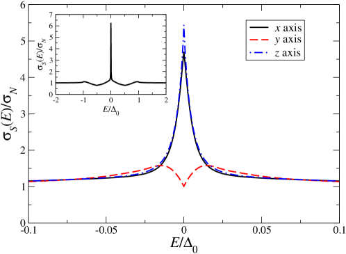
Figure 5: Normalized conductance spectra close to zero bias at the $(101)$ surface of a three-dimensional NCS with $C_{4v}$ point group. The curves show the dependence of the tunneling conductance on the orientation of the magnetization of the insulating tunnel barrier, which is modeled by the parameters $Z_{c}=4$ and $Z_{s}=1$. We ignore the effect of spin-orbit splitting in the NCS and set $q=0.25$. Inset: normalized conductance spectrum over a larger range of energies for a nonmagnetic barrier with $Z_{c}=4$ and $Z_{s}=0$; turning on the magnetic potential does not significantly modify the conductance spectra outside the energy range in the immediate vicinity of the zero-bias conduction peak.

In figure 5 we plot the conductance normalized by the normal-state value $\sigma_{N}$ for tunneling through the (101) surface of a $C_{4v}$ NCS. As shown in the inset, the conductance spectrum for a nonmagnetic tunnel barrier is dominated by a sharp peak at zero bias, which arises from resonant tunneling through the zero-energy flat-band states, which are now resonances in the NCS due to the nonzero barrier transparency [11, 12]. Upon switching on the barrier magnetization, the peak remains intact for a magnetization in the $xz$ plane but disappears completely for a magnetization along the $y$ axis. The conductance spectrum at larger bias is essentially unaffected by the barrier magnetization. This behavior results from the coupling of the barrier magnetization to the surface spin density of the nondegenerate flat-band resonances. A naive perturbative argument implies that the energy of the resonance should be shifted by an amount proportional to the surface spin polarization. Shifting the resonance away from zero energy results in a reduction of the conductance peak at zero bias, which is indeed observed in figure 5. We remark that the strong dependence of the tunneling conductance on the orientation of the barrier magnetization, which is shown in figure 5, is qualitatively different from the behavior of the tunneling conductance in an equivalent junction involving a singlet $d$-wave superconductor. In the latter case, the ferromagnetic tunnel barrier splits the spin-degenerate surface states of the superconductor for arbitrary orientations of the barrier magnetization, which in turn leads to a suppression of the zero-bias conductance independent of this orientation [45].

Although the surface spin density is not equivalent to the total spin polarization, we nevertheless find the latter to be a good guide to the fate of the zero-bias peak. Examining the spin polarization for the states at the (101) surface of the $C_{4v}$ NCS in figures 4(f)–(h), we see that the absence of the zero-bias peak for a $y$-polarized barrier but its presence for a $z$-polarized barrier is consistent with the strong spin polarization of the surface states along the $y$ axis and the vanishing spin polarization along the $z$ axis. Although the height of the zero-bias peak for an $x$-polarized barrier is approximately 15% smaller than for the $z$-polarized barrier, the survival of the zero-bias peak in spite of the strong $x$-spin polarization of the surface states is somewhat surprising. A possible explanation is that the states with the strongest $x$-spin polarization have surface momenta close to the projected nodal lines, and thus have diverging localization lengths. This strongly suppresses their weight at the tunnel barrier, and hence their energy shift due to the coupling to the barrier moment is also reduced.

Figure 6: Variation of the zero-bias conductance as a function of the orientation of the barrier magnetization for (a) a $C_{2}$ NCS at the (100) surface, (b) a $C_{4v}$ NCS at the (101) surface, and (c) a $O$ NCS at the (111) surface. The position on the surface of the one-eighth sphere represents the orientation of the magnetization, while the color at each point gives the ratio of the zero-bias conductance to the maximum value. In all panels we set $q=0.25$, $Z_{c}=4$, and $Z_{s}=1$.

The dependence of the zero-bias conductance on the orientation of the barrier magnetization is shown in figure 6 for the three NCS point groups considered in section 4. In all cases we find not only a strong variation of the conductance as a function of the orientation but also observe that this dependence is distinctly different for each point group. This can be exploited to test the existence of spin-polarized flat bands and also to identify the pairing symmetry of the NCS.

6 Summary and outlook

In this work we have presented a systematic study of the spin polarization of NCS surface states using quasiclassical scattering theory. Examining both fully gapped and nodal pairing states, we have shown how the spin polarization generally depends on the interplay of spin-orbit coupling and singlet-triplet pairing ratio in the superconductor. The variation of the surface-state spin polarization strongly reflects the relative weight of negative- and positive-helicity wavefunction components and is to some degree controlled by the spin polarization of the bulk states at the point where the surface states connect to the bulk continuum. This is particularly pronounced in nodal NCSs, where the spin polarization of the surface states evolves to match that of the normal states at the gap nodes. We have also shown that the spin polarization of the surface states can be directly probed in a tunnel junction consisting of a normal metal and an NCS separated by an insulating ferromagnetic barrier. Specifically, the dependence of the zero-bias conductance on the orientation of the barrier magnetization is a signature of spin-polarized flat-band surface states.

Our results provide a deeper understanding of the surface physics of NCS, which reflects the topological properties of these materials. Although the spin polarization of the surface states is not directly related to their topology, it can nevertheless be exploited in experiments to detect the topological surface states and to probe their degeneracy. We believe that our findings will prove relevant for designing experiments to test the topological character of NCS and other unconventional superconductors. While we have focused in this work on NCSs with one spin-split Fermi surface, our analysis can be generalized in a straightforward manner to other topological superconductors [1], e.g., centrosymmetric systems with triplet pairing, locally noncentrosymmetric superconductors [46, 47], Weyl superconductors [48], and superconductors with multiple spin-split Fermi sheets.

References

References

- [1] Schnyder A P, Ryu S, Furusaki A and Ludwig A W W 2008 Phys. Rev. B 78(19) 195125
- [2] Kitaev A 2009 AIP Conference Proceedings 1134 22–30
- [3] Schnyder A P, Ryu S, Furusaki A and Ludwig A W W 2009 AIP Conference Proceedings 1134 10–21
- [4] Hasan M Z and Kane C L 2010 Rev. Mod. Phys. 82(4) 3045–3067
- [5] Ryu S, Schnyder A P, Furusaki A and Ludwig A W W 2010 New Journal of Physics 12 065010
- [6] Qi X L and Zhang S C 2011 Rev. Mod. Phys. 83(4) 1057–1110
- [7] Sato M 2006 Phys. Rev. B 73(21) 214502
- [8] Yada K, Sato M, Tanaka Y and Yokoyama T 2011 Phys. Rev. B 83(6) 064505
- [9] Schnyder A P and Ryu S 2011 Phys. Rev. B 84(6) 060504
- [10] Schnyder A P, Brydon P M R and Timm C 2012 Phys. Rev. B 85(2) 024522
- [11] Brydon P M R, Schnyder A P and Timm C 2011 Phys. Rev. B 84(2) 020501
- [12] Tanaka Y, Mizuno Y, Yokoyama T, Yada K and Sato M 2010 Phys. Rev. Lett. 105(9) 097002
- [13] Dahlhaus J P, Gibertini M and Beenakker C W J 2012 Phys. Rev. B 86(17) 174520
- [14] Matsuura S, Chang P Y, Schnyder A P and Ryu S 2013 New Journal of Physics 15 065001
- [15] Sato M and Fujimoto S 2009 Phys. Rev. B 79(9) 094504
- [16] Qi X L, Hughes T L and Zhang S C 2010 Phys. Rev. B 81(13) 134508
- [17] Yip S K 2010 Journal of Low Temperature Physics 160 12–31 ISSN 0022-2291
- [18] Tanaka Y, Yokoyama T, Balatsky A V and Nagaosa N 2009 Phys. Rev. B 79(6) 060505
- [19] Sato M, Tanaka Y, Yada K and Yokoyama T 2011 Phys. Rev. B 83(22) 224511
- [20] Tanaka Y, Sato M and Nagaosa N 2012 Journal of the Physical Society of Japan 81 011013
- [21] Bauer E and Sigrist M 2012 Non-Centrosymmetric Superconductors: Introduction and Overview (Lecture Notes in Physics vol 847) (Springer Berlin)
- [22] Yuan H Q, Agterberg D F, Hayashi N, Badica P, Vandervelde D, Togano K, Sigrist M and Salamon M B 2006 Phys. Rev. Lett. 97(1) 017006
- [23] Nishiyama M, Inada Y and Zheng G q 2007 Phys. Rev. Lett. 98(4) 047002
- [24] Joshi B, Thamizhavel A and Ramakrishnan S 2011 Phys. Rev. B 84(6) 064518
- [25] Mondal M, Joshi B, Kumar S, Kamlapure A, Ganguli S C, Thamizhavel A, Mandal S S, Ramakrishnan S and Raychaudhuri P 2012 Phys. Rev. B 86(9) 094520
- [26] Matano K, Maeda S, Sawaoka H, Muro Y, Takabatake T, Joshi B, Ramakrishnan S, Kawashima K, Akimitsu J and qing Zheng G 2013 Journal of the Physical Society of Japan 82 084711
- [27] Bauer E, Hilscher G, Michor H, Paul C, Scheidt E W, Gribanov A, Seropegin Y, Noël H, Sigrist M and Rogl P 2004 Phys. Rev. Lett. 92(2) 027003
- [28] Sugitani I, Okuda Y, Shishido H, Yamada T, Thamizhavel A, Yamamoto E, Matsuda T D, Haga Y, Takeuchi T, Settai R and Ōnuki Y 2006 J. Phys. Soc. Jpn. 75 043703
- [29] Iniotakis C, Hayashi N, Sawa Y, Yokoyama T, May U, Tanaka Y and Sigrist M 2007 Phys. Rev. B 76(1) 012501
- [30] Vorontsov A B, Vekhter I and Eschrig M 2008 Phys. Rev. Lett. 101(12) 127003
- [31] Lu C K and Yip S 2010 Phys. Rev. B 82(10) 104501
- [32] Brydon P M R, Timm C and Schnyder A P 2013 New Journal of Physics 15 045019
- [33] Schnyder A P, Timm C and Brydon P M R 2013 Phys. Rev. Lett. 111(7) 077001
- [34] Hofmann J S, Queiroz R and Schnyder A P 2013 Phys. Rev. B 88(13) 134505
- [35] Wong C L M, Liu J, Law K T and Lee P A 2013 Phys. Rev. B 88(6) 060504
- [36] Frigeri P A, Agterberg D F, Koga A and Sigrist M 2004 Phys. Rev. Lett. 92(9) 097001
- [37] Samokhin K 2009 Annals of Physics 324 2385–2407
- [38] Bauer E, Rogl G, Chen X Q, Khan R T, Michor H, Hilscher G, Royanian E, Kumagai K, Li D Z, Li Y Y, Podloucky R and Rogl P 2010 Phys. Rev. B 82(6) 064511
- [39] Karki A B, Xiong Y M, Vekhter I, Browne D, Adams P W, Young D P, Thomas K R, Chan J Y, Kim H and Prozorov R 2010 Phys. Rev. B 82(6) 064512
- [40] Queiroz R and Schnyder A P 2014 Phys. Rev. B 89(5) 054501
- [41] Agterberg D F and Kaur R P 2007 Phys. Rev. B 75(6) 064511
- [42] Loder F, Kampf A P and Kopp T 2013 Journal of Physics: Condensed Matter 25 362201
- [43] Blonder G E, Tinkham M and Klapwijk T M 1982 Phys. Rev. B 25(7) 4515–4532
- [44] Yokoyama T, Tanaka Y and Inoue J 2005 Phys. Rev. B 72(22) 220504
- [45] Kashiwaya S, Tanaka Y, Yoshida N and Beasley M R 1999 Phys. Rev. B 60(5) 3572–3580
- [46] Biswas P K, Luetkens H, Neupert T, Stürzer T, Baines C, Pascua G, Schnyder A P, Fischer M H, Goryo J, Lees M R, Maeter H, Brückner F, Klauss H H, Nicklas M, Baker P J, Hillier A D, Sigrist M, Amato A and Johrendt D 2013 Phys. Rev. B 87(18) 180503
- [47] Fischer M H, Neupert T, Platt C, Schnyder A P, Hanke W, Goryo J, Thomale R and Sigrist M 2014 Phys. Rev. B 89(2) 020509
- [48] Meng T and Balents L 2012 Phys. Rev. B 86(5) 054504