Surface transport coefficients for three-dimensional topological superconductors

Abstract

We argue that surface spin and thermal conductivities of three-dimensional topological superconductors are universal and topologically quantized at low temperature. For a bulk winding number $\nu$, there are $|\nu|$ “colors” of surface Majorana fermions. Localization corrections to surface transport coefficients vanish due to time-reversal symmetry (TRS). We argue that Altshuler-Aronov interaction corrections vanish because TRS forbids color or spin Friedel oscillations. We confirm this within a perturbative expansion in the interactions, and to lowest order in a large-$|\nu|$ expansion. In both cases, we employ an asymptotically exact treatment of quenched disorder effects that exploits the chiral character unique to two-dimensional, time-reversal-invariant Majorana surface states.

I Introduction

In the quantum Hall effect, transport measurements unambiguously reveal the chiral edge states. The precisely quantized Hall conductance is a topological quantum number that is insensitive to the sample geometry and protected from the effects of disorder or interactions. Transport has played a lesser role in the characterization of three-dimensional (3D) topological insulators, in part because it has proven difficult to separate bulk and surface contributions due to unintended doping QZ2011 . A more fundamental limitation is that transport coefficients do not directly reflect the $\mathbb{Z}_{2}$ topological invariant when time-reversal symmetry (TRS) is preserved. Instead, the Dirac surface states of topological insulators are distinguished by the absence of a two-dimensional (2D) metal-insulator transition, with a disorder-dependent electrical conductivity that flows to ever larger values on longer scales due to weak antilocalization Bardarson07 ; Nomura07 ; QGM2010 ; footnote–TIwithInts .

In this paper, we show that 3D topological superconductors (TSCs) HK2010 ; QZ2011 ; SRFL2008 ; Kit ; RSFL2010 ; Foster2012 ; FXCup may provide a closer analog of the 2D quantum Hall effect. A bulk TSC is characterized by an integer-valued winding number $\nu$, and belongs to one of three classes CI, AIII, or DIII SRFL2008 . At the surface, there are $|\nu|$ degenerate species (or “colors”) of surface Majorana fermion bands SRFL2008 ; FXCup . These are protected by TRS in all three classes. We will argue that surface transport coefficients (spin and thermal conductivities) are universal, being determined only by the bulk winding number. An important consequence is that low-temperature surface spin and heat transport can provide a “smoking gun” for Majorana surface states.

For a TSC with conserved spin and no interactions, it is known that the zero-temperature ($T=0$) spin conductivity is unmodified by nonmagnetic disorder ludwig1994 ; Tsv1995 ; mirlin2006 . Without interactions, the ratio of the thermal conductivity to temperature is also universal in the limit $T\rightarrow 0$ SRFL2008 ; FXCup . These results are insufficient to establish universal transport, however, because interactions usually induce Altshuler-Aronov (AA) conductance corrections in the presence of disorder AA1985 . These occur due to carrier scattering off of self-consistent potential fluctuations AAG99 ; ZNA2001 , and can even cause Anderson localization AA1985 ; Finkel1983 ; BK1994 .

Here we argue that all interaction corrections to TSC surface transport coefficients vanish. The physical picture is simple: disorder cannot induce static modulations in the color, spin, or mass densities of the surface Majorana fluid unless time-reversal symmetry is broken (externally or spontaneously). Then there is no mechanism for short-ranged interactions to relax momentum at zero temperature. To support our claim, we show that perturbative interaction corrections to the surface spin conductivity vanish in every disorder realization. We also show that AA corrections to the spin and thermal surface conductances vanish to leading order in a large winding number expansion. The quantization of surface transport coefficients hints at a deeper topological origin, which we will contemplate in the conclusion.

The results in the absence of interactions are as follows. In a system in which spin is at least partially conserved (classes CI and AIII SRFL2008 ; Kit ; RSFL2010 ; FXCup ), spin transport is well-defined. Both spin and heat can be conducted by the Majorana surface bands. Neglecting interactions, the $T=0$ surface spin conductivity assumes the universal value ludwig1994 ; Tsv1995 ; mirlin2006

$$\sigma_{xx}^{\mathrm{s}}=\frac{|\nu|}{\pi h}\left(\frac{\hbar}{2}\right)^{2},\;\;\text{classes CI and AIII},$$ (1)

where $\nu\in\mathbb{Z}$ ($2\mathbb{Z}$) denotes the bulk winding number for class AIII (CI) TSCs. If spin is not conserved due to spin-orbit coupling (class DIII), the Majorana surface states still conduct energy. The low temperature thermal conductivity is

$$\kappa_{xx}=\frac{|\nu|}{\pi h}\frac{\pi^{2}k_{\mathrm{B}}^{2}T}{3\gamma},\;\;\gamma=\left\{\begin{array}[]{ll}1,&\text{classes CI and AIII,}\\ 2,&\text{class DIII.}\end{array}\right.$$ (2)

Equation (2) follows from the Wiedemann-Franz law SF2000 ; SRFL2008 ; NRFN2012 ; Nakai2014 ; FXCup .

Interactions play a dual role in quantum transport AAG99 . On one hand, real inelastic scattering cuts off quantum interference at finite temperature, suppressing weak localization on scales larger than the dephasing length. Interference corrections are absent in a TSC, but interactions could modify transport coefficients in another way.

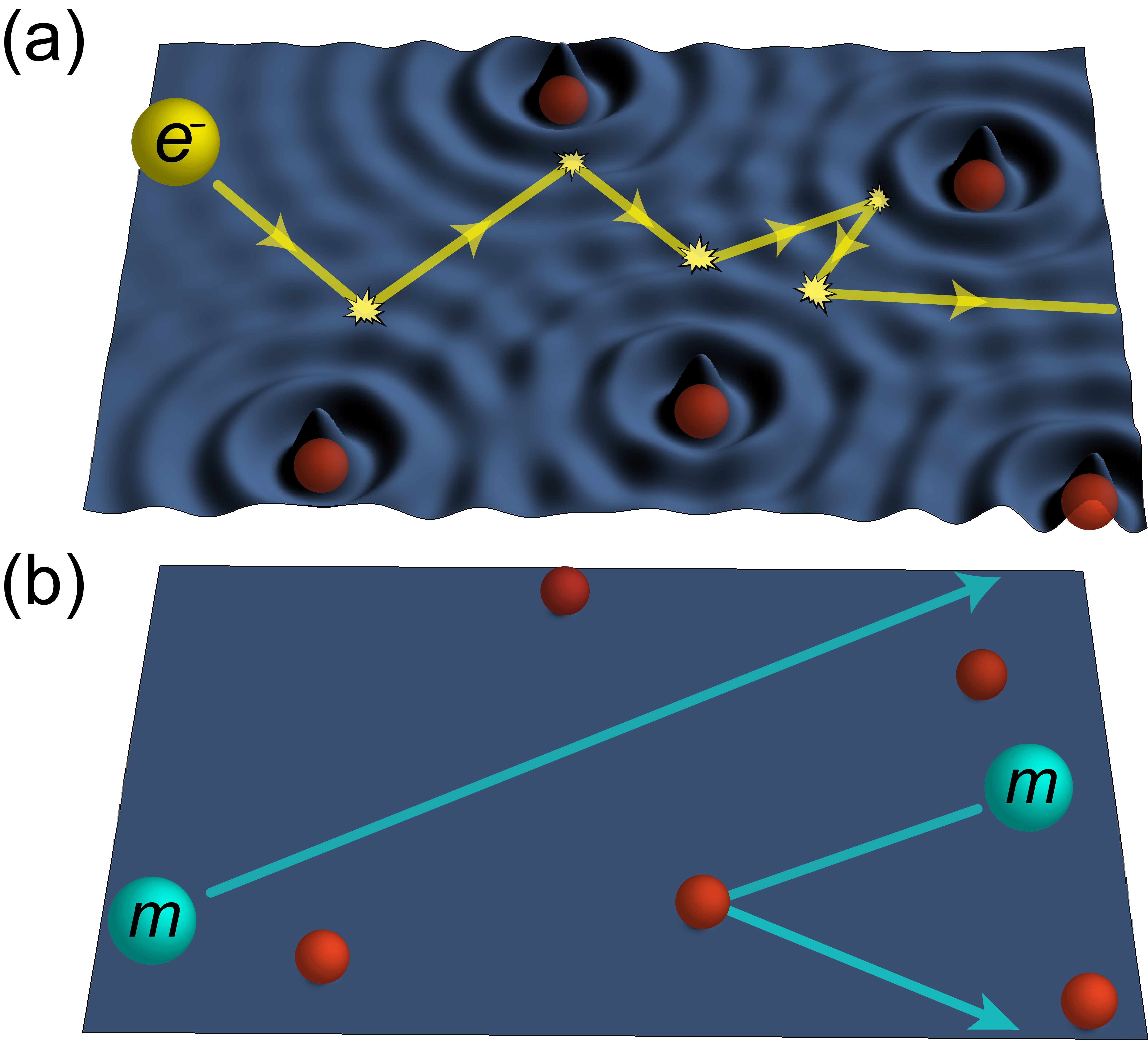
Figure 1: In a disordered metal (a), electrons scatter off of both impurities and density Friedel oscillations; the latter produce Altshuler-Aronov (AA) quantum conductance corrections AA1985 ; AAG99 ; ZNA2001 . The Majorana fluid (b) at the surface of a TSC remains featureless in any realization of nonmagnetic disorder, as no relevant (spin, mass, or color) density can become nonzero without breaking time-reversal symmetry. We therefore expect that surface transport coefficients for bulk TSCs are free of AA corrections. By contrast, AA corrections are ubiquitous in other 2D Dirac systems, including the surface states of 3D topological insulators QGM2010 , and nodal quasiparticles in time-reversal invariant, nontopological superconductors MJeng2001 ; DellAnna2002 ; dellanna2006 ; foster0608 .

Disorder induces inhomogeneous fluctuations in single-particle wave functions, and these can produce density oscillations near impurities. AA conductance corrections AA1985 arise due to the coherent scattering of electrons off of the self-consistent potential due to these oscillations AAG99 ; ZNA2001 . These corrections are ubiquitous in both the standard Wigner-Dyson AA1985 ; Finkel1983 ; BK1994 and exceptional Altland-Zirnbauer wm2008 classes, including nontopological superconductors MJeng2001 ; DellAnna2002 ; dellanna2006 ; foster0608 . AA corrections can induce Anderson localization even when the noninteracting system would remain metallic. For example, in a 2D electron gas with strong spin-orbit scattering, the correction to the electric conductance due to Coulomb interactions overwhelms weak antilocalization BK1994 in the diffusive regime. This is precisely what happens for a single surface state band enveloping a 3D topological insulator with a properly insulating bulk. In that case delocalization may survive at a strongly coupled fixed point QGM2010 ; footnote–TIwithInts .

In a 3D TSC, the physics is uniquely different, owing to the anomalous form that TRS assumes at the surface SRFL2008 ; Foster2012 ; FXCup . Nonmagnetic disorder couples only to the color or spin currents of the $|\nu|$-fold degenerate Majorana quasiparticle bands SRFL2008 ; FXCup . Disorder cannot induce static oscillations in the color or spin densities so long as TRS is preserved. Mass terms for the Majorana bands are also forbidden. Interactions can renormalize the existing disorder profile, but this does not modify transport coefficients in a TSC.

In this paper, we argue that interaction corrections vanish to all orders, due to the featureless character of the surface Majorana fluid; see Fig. 1. To support this argument, we explicitly verify that Eqs. (1) and (2) are unmodified by interactions in two limits. First we show that the interaction contributions to the $T=0$ surface spin conductivity vanish in every disorder realization for classes CI and AIII. We demonstrate this to first (second) order for class CI (AIII), and sketch an all-orders proof for AIII. Then we consider a large winding number ($|\nu|\gg 1$) expansion, using the Wess-Zumino-Novikov-Witten Finkel’stein nonlinear sigma models (WZNW-FNLsMs) introduced in Ref. FXCup . We find that the AA corrections to the spin (CI, AIII) or thermal (DIII) conductances are suppressed in the conformal limit for all three TSC classes, to the lowest nontrivial order in $1/|\nu|$. An important caveat that we do not address here is whether nonsingular interaction corrections arise to the thermal conductivity that violate the Wiedemann-Franz relation in classes CI and AIII CA2005 .

This paper is organized as follows. In Sec. II we define models and present the results of our calculations. We qualitatively sketch the key elements responsible for the cancellation of AA corrections in both schemes, without getting into details. We also discuss implications and open questions. The rest of the paper consists of three technical sections that are mutually independent. In Sec. III we construct a lattice model for a class AIII topological superconductor, and derive the form of the surface state theory assumed in Sec. II. We present the calculation of Altshuler-Aronov corrections to the surface spin conductivity using the Kubo formula in Sec. IV. Finally we derive the WZNW-FNLsM results in Sec. V.

II Approach and main results

II.1 Majorana surface bands

The key signature of a 3D TSC with a winding number $\nu$ is the presence of gapless quasiparticle bands at the surface SRFL2008 ; Kit ; RSFL2010 . At energies below the bulk superconducting gap, these can be viewed as $|\nu|$ “colors” of surface Majorana fermions. The surface states near zero energy measured relative to the bulk chemical potential are protected from the opening of a gap and from Anderson localization, so long as TRS is preserved SRFL2008 ; FXCup . The three 3D TSC classes differ by the amount of spin rotational symmetry preserved in the bulk and at the surface. Classes CI, AIII, and DIII respectively possess spin SU(2), spin U(1), and no spin symmetry.

The low-energy effective field theory SRFL2008 ; FXCup for noninteracting Majorana surface bands is given by

$$\begin{split}H^{(0)}=&\,\int\!\mathrm{d}^{2}\mathbf{r}\,\eta^{\dagger}(\mathbf{r})\,\hat{h}\,\eta(\mathbf{r}),\\ \hat{h}=&\,\hat{\bm{\sigma}}\cdot\left[-i\bm{\nabla}+\mathbf{A}_{j}(\mathbf{r})\,\hat{\mathfrak{t}}^{j}+{\bm{\mathcal{A}}}(\mathbf{r})\right].\end{split}$$ (3)

In Eq. (3), $\eta\rightarrow\eta_{\sigma,\kappa}$ is a fermion field with indices in pseudospin $\sigma\in\{1,2\}$ and color $\kappa\in\{1,2,\cdots,|\nu|\}$ spaces; here $\hat{\bm{\sigma}}=\{\hat{\sigma}^{1},\hat{\sigma}^{2}\}$ denotes the vector of pseudospin Pauli matrices. The pseudospin degree of freedom is some admixture of Nambu (particle-hole), orbital, and in the case of class DIII physical spin-$1/2$ spaces SRFL2008 ; FB2010 ; FXCup ; YSTY2011 ; YYST2012 . A bulk microscopic model is necessary to fix the interpretation, but not the structure of the theory. The potentials $\mathbf{A}_{j}$ and ${\bm{\mathcal{A}}}$ encode quenched disorder, as defined below.

For classes CI and AIII, $\eta(\mathbf{r})$ is a complex-valued Dirac spinor; the U(1) charge is the conserved spin projection along the $z$-spin axis SRFL2008 ; FXCup . The U(1) current encodes the $z$-spin density and associated spin current

$$\eta^{\dagger}\eta(\mathbf{r})=2S^{z}(\mathbf{r}),\quad\eta^{\dagger}\,\hat{\bm{\sigma}}\,\eta(\mathbf{r})=2\mathbf{J}^{z}(\mathbf{r}).$$ (4)

By contrast, in class DIII $\eta(\mathbf{r})$ is a real spinor that can be taken to satisfy FXCup $\eta^{\dagger}=-i\eta^{\mathsf{T}}\hat{\sigma}^{1}.$ Only the energy density and energy current (components of the energy-momentum tensor) are conserved in class DIII.

As is typical for a topological phase HK2010 ; QZ2011 , symmetries are implemented in an anomalous fashion at the surface of a 3D TSC. In particular, TRS appears as the chiral condition SRFL2008 ; FXCup ; BerLec2002

$$-\hat{\sigma}^{3}\,\hat{h}\,\hat{\sigma}^{3}=\hat{h}.$$ (5)

Given our basis choice, Eq. (5) is unique SRFL2008 and implies that external time-reversal invariant perturbations appear in the surface theory as vector potentials. In particular, for a system with $|\nu|\geq 2$ colors and spin SU(2) symmetry, nonmagnetic disorder induces intercolor scattering in the form of the non-Abelian potential $A_{j}^{\alpha}(\mathbf{r})\,\hat{\mathfrak{t}}^{j}$ $(\alpha\in\{1,2\})$ in Eq. (3) footnote–charge density . The color space symmetry generators $\{\hat{\mathfrak{t}}^{j}\}$ satisfy a particular Lie algebra $G(|\nu|)$ for each TSC class footnote–LAclasses . In addition, class AIII admits the abelian vector disorder potential $\mathcal{A}^{\alpha}(\mathbf{r})$, which couples to the U(1) spin current in Eq. (3). This term is forbidden by spin SU(2) symmetry in class CI FXCup , and vanishes exactly for DIII. TRS also forbids the accumulation of nonzero spin or color densities. We denote the spin density as $\mathbf{S}(\mathbf{r})$. In classes CI and AIII, the $z$ component is defined above in Eq. (4). The non-Abelian color density is $\eta^{\dagger}\hat{\mathfrak{t}}^{j}\eta(\bm{\mathrm{r}})$. The complete set of Hermitian fermion bilinears (without derivatives) also includes mixed spin-color potentials, as well as Dirac mass operators FXCup . All of these are odd under time reversal.

We illustrate these key attributes of TSC surface states in Sec. III. Starting from a bulk microscopic model, we derive Eqs. (3) and (5) for the Majorana surface fluid of a class AIII TSC.

To treat interactions, we enumerate four-fermion terms consistent with bulk time-reversal and spin symmetries. We do not consider long-ranged Coulomb interactions since these should be screened by the bulk superfluid. We also neglect interactions that break color symmetry, but our results are independent of this.

For class CI (AIII), because spin SU(2) [U(1)] symmetry is preserved, we expect a spin exchange interaction of the type $\mathbf{S}(\mathbf{r})\cdot\mathbf{S}(\mathbf{r})$ [$S^{z}(\mathbf{r})S^{z}(\mathbf{r})$] is important. In all three classes, TRS implies that a BCS interaction could induce a pairing instability at the surface. The Dirac mass operator $m(\mathbf{r})=\eta^{\dagger}\,\hat{\sigma}^{3}\,\eta(\mathbf{r})$ is time-reversal odd, and $\langle m(\mathbf{r})\rangle\neq 0$ means opening a gap. The mass term can be interpreted as an imaginary surface pairing amplitude. For example, in class CI this is the spin singlet operator Foster2012 ; FXCup $m(\mathbf{r})\sim-i\,C_{\uparrow}^{\dagger}(\mathbf{r})\,C_{\downarrow}^{\dagger}(\mathbf{r})+i\,C_{\downarrow}(\mathbf{r})\,C_{\uparrow}(\mathbf{r})$, where $C_{\mu}(\mathbf{r})$ annihilates an electron. We therefore can write an attractive BCS interaction as $\sim-m^{2}(\mathbf{r})$. The interacting Hamiltonian in each class takes the form FXCup

$$H_{\text{CI}}^{(I)} =\int\!\mathrm{d}^{2}\mathbf{r}\,\left[\Gamma_{\mathrm{s}}\,\mathbf{S}(\mathbf{r})\cdot\mathbf{S}(\mathbf{r})+\Gamma_{\mathrm{c}}\,m(\mathbf{r})\,m(\mathbf{r})\right],$$ (6a)

$$H_{\text{AIII}}^{(I)} =\int\!\mathrm{d}^{2}\mathbf{r}\,\left[\Gamma_{\mathrm{s}}\,S^{z}(\mathbf{r})\,S^{z}(\mathbf{r})+\Gamma_{\mathrm{c}}\,m(\mathbf{r})\,m(\mathbf{r})\right],$$ (6b)

$$H_{\text{DIII}}^{(I)} =\int\!\mathrm{d}^{2}\mathbf{r}\,\Gamma_{\mathrm{c}}\,m(\mathbf{r})\,m(\mathbf{r}),$$ (6c)

where $\Gamma_{\mathrm{s}}$ and $\Gamma_{\mathrm{c}}$ are repulsive spin exchange and BCS pairing interaction strengths, respectively.

II.2 Spin conductivity, interaction expansion

The spin conductivity in Eq. (1) is simply the $T=0$ ballistic Landauer result expected for $|\nu|$ species of 2D noninteracting, massless Dirac fermions ludwig1994 ; TTTRB ; RMFL2007 ; MBT2009 . Here the electric charge $e$ is replaced with the spin quantum $\hbar/2$. That Eq. (1) holds in the presence of disorder Tsv1995 ; mirlin2006 is due to the chiral symmetry in Eq. (5), which is just TRS for the surface state quasiparticles SRFL2008 ; FXCup . The chiral symmetry allows the retarded (R) and advanced (A) single-particle Green’s functions to be interchanged,

$$-\hat{\sigma}^{3}\,\hat{G}^{R/A}({\epsilon};\bm{\mathrm{r}},\bm{\mathrm{r^{\prime}}})\,\hat{\sigma}^{3}=\hat{G}^{A/R}(-{\epsilon};\bm{\mathrm{r}},\bm{\mathrm{r^{\prime}}}).$$ (7)

Using Eq. (7), the noninteracting Kubo formula can be written in terms of a product of retarded Green’s functions. The Ward identity [Eq. (54)] can then be used to reduce this to the short-distance limit of a single function,

$$\sigma_{xx}^{\mathrm{s}}=-\frac{1}{4\pi}\lim_{\bm{\mathrm{r}}\rightarrow\bm{\mathrm{r^{\prime}}}}\text{Im}\left\{\textrm{Tr}\left[\bm{\sigma}\cdot(\bm{\mathrm{r}}-\bm{\mathrm{r^{\prime}}})\,\hat{G}^{R}(0;\bm{\mathrm{r}},\bm{\mathrm{r^{\prime}}})\right]\right\}.$$

Although this expression must be properly regularized, it is clear that the dc conductivity is dominated by the ultraviolet, and is independent of the disorder [which affects $\hat{G}^{R}({\epsilon};\bm{\mathrm{r}},\bm{\mathrm{r^{\prime}}})$ only on scales larger than the mean-free path]. The correct noninteracting result in Eq. (1) can be understood as a consequence of the axial anomaly in 2+0-D mirlin2006 .

For classes CI and AIII, Eq. (2) follows from Eq. (1) via the Wiedemann-Franz relation. Alternatively, one can obtain Eq. (2) using the Landauer formula for the thermal conductance of 2D ballistic Dirac fermions, doped to the Dirac point TTTRB ; RMFL2007 ; MBT2009 . We argued in Ref. FXCup that Eq. (2) with $\gamma=2$ holds for class DIII, wherein spin is not conserved. This is derived by artificially doubling the theory to obtain a fictitious U(1) charge and applying Wiedemann-Franz to Eq. (1), and then halving this result. See also Refs. SF2000 ; NRFN2012 ; Nakai2014 .

Figure 2: First-order Hartree (a) and Fock (b) interaction corrections to the spin conductivity in classes CI and AIII, and examples of second-order corrections [(c), (d)] for class AIII. The dashed lines indicate the spin current operators. The solid lines represent the exact noninteracting Matsubara Green’s functions in an arbitrary, fixed realization of quenched surface disorder. The wavy lines correspond to the interaction potentials. Both current operators and interaction potentials are local in space. Panels (c) and (d) depict categories of second-order corrections that are subleading in the inverse winding number. Each correction in (a) and (b) vanishes individually, while those in each category (c) and (d) sum to zero. In Sec. IV.2, we show that a similar cancellation occurs for all second-order corrections. We sketch a proof that the same mechanism works to all orders in Sec. IV.3, implying that Altshuler-Aronov corrections do not exist for Majorana surface transport coefficients.

For classes CI and AIII, the surface spin conductivity $\sigma_{xx}^{\mathrm{s}}$ obtains via the Kubo formula. For a fixed realization of disorder, the leading order interaction (Hartree-Fock) corrections are represented by the Feynman diagrams in Figs. 2(a) and 2(b). In Sec. IV, we show that short-ranged interactions do not contribute to $\sigma_{xx}^{\mathrm{s}}$ in the Hartree-Fock approximation, at zero temperature. The Hartree terms a(i) and a(ii) and the Fock terms b(i) and b(ii) vanish individually due to the chirality of the Green’s functions, Eq. (7). The terms a(iii) and b(iii) do not contribute to $\sigma_{xx}^{\mathrm{s}}$ due to the Ward identity. The absence of Hartree-Fock corrections is distinct from the Fermi liquid case AA1985 ; AAG99 ; ZNA2001 .

We compute all second-order corrections for class AIII, and find that these vanish as well. These calculations are detailed in Sec. IV.2. The main idea is that $\sigma_{xx}^{\mathrm{s}}$ corrections can be grouped into classes, with each class corresponding to a particular “free energy” bubble. Examples of two such classes are the second-order groups (c) and (d) shown in Fig. 2. The corrections in each class sum over all possible ways of inserting two current operators into the bubble, but this sum vanishes. This is because AA corrections at $T=0$ only involve Green’s functions at zero energy, so that retarded and advanced versions are equivalent [Eq. (7)]. The Ward identity then implies that a sum over diagrams reduces to a sum over the relative positions of interaction vertices in a free energy bubble, and this is equal to zero. We sketch a proof that all higher-order corrections vanish via the same mechanism in Sec. IV.3.

II.3 Spin and thermal conductivities, large winding number expansion

We also compute interaction corrections in a large winding number expansion, employing the WZNW-FNLsMs FXCup for the interacting surface Dirac fermions described by Eqs. (3) and (6). These low-energy effective field theories are derived directly from the non-Abelian bosonization of the Dirac fermions, without recourse to the self-consistent Born approximation or a gradient expansion. In each class, the model contains a parameter $\lambda$ that is proportional to the dimensionless spin (thermal) resistance in classes CI and AIII (DIII). The universal transport coefficients in Eqs. (1) and (2) obtain for the noninteracting models tuned to a conformal fixed point such that $\lambda=1/K$, where $K=|\nu|$ ($K=|\nu|/2$) in classes AIII and DIII (CI). The models are defined explicitly in Sec. V, Eqs. (106)–(117).

Perturbing the sigma models around the noninteracting conformal fixed point, we derive the following one-loop RG equations for $\lambda$ in Sec. V:

$$\text{CI:}\quad d\lambda/dl= \,\lambda^{2}\left[1-(K\lambda)^{2}\right][1+\mathcal{J}(\gamma_{\mathrm{s}},\gamma_{\mathrm{c}})],$$ (8a)

$$\text{AIII:}\quad d\lambda/dl= \,\lambda^{2}\left[1-(K\lambda)^{2}\right]\mathcal{I}(\gamma_{\mathrm{s}},\gamma_{\mathrm{c}}),$$ (8b)

$$\text{DIII:}\quad d\lambda/dl= \,-\lambda^{2}\left[1-(K\lambda)^{2}\right][2+\mathcal{K}\left(\gamma_{\mathrm{c}}\right)].$$ (8c)

In Eq. (8), $\gamma_{\mathrm{s}}$ and $\gamma_{\mathrm{c}}$ are rescaled versions of the interaction strengths that appear in Eq. (6), $\gamma_{\mathrm{s},\mathrm{c}}=4\,\Gamma_{\mathrm{s},\mathrm{c}}/\pi h,$ where $h$ is a sigma model parameter that couples to frequency [Eqs. (109) and (113)]. The functions $\mathcal{J}$, $\mathcal{I}$, and $\mathcal{K}$ are defined as

$$\!\!\mathcal{J}(\gamma_{\mathrm{s}},\gamma_{\mathrm{c}}) =\textstyle{3\left[1+\frac{1-\gamma_{\mathrm{s}}}{\gamma_{\mathrm{s}}}\ln{(1-\gamma_{\mathrm{s}})}\right]-\frac{1}{4}\mathcal{K}(\gamma_{\mathrm{c}})},$$ (9a)

$$\!\!\mathcal{I}(\gamma_{\mathrm{s}},\gamma_{\mathrm{c}}) =\textstyle{2\left[1+\frac{1-\gamma_{\mathrm{s}}}{\gamma_{\mathrm{s}}}\ln{(1-\gamma_{\mathrm{s}})}\right]-\frac{1}{2}\mathcal{K}(\gamma_{\mathrm{c}})},$$ (9b)

$$\!\!\mathcal{K}(\gamma_{\mathrm{c}}) =\textstyle{2e^{-1/\gamma_{\mathrm{c}}}\left[E_{i}\left(\frac{1}{\gamma_{\mathrm{c}}}+\ln 2\right)-E_{i}\left(\frac{1}{\gamma_{\mathrm{c}}}\right)\right]}\!,$$ (9c)

and represent the AA corrections Finkel1983 ; dellanna2006 ; AA1985 ; BK1994 . Here $E_{i}(z)$ denotes the exponential integral function. For class AIII, there is an additional equation for the parameter $\lambda_{A}$ [see Eqs. (113) and (115)], which governs the strength of the Abelian random potential ${\bm{\mathcal{A}}}(\mathbf{r})$ in Eq. (3):

$$d\lambda_{\mathrm{A}}/dl=\,\textstyle{\lambda^{2}\left[1-(K\lambda)^{2}\right]\left[1+\frac{2\lambda_{\mathrm{A}}}{\lambda}\mathcal{I}(\gamma_{\mathrm{s}},\gamma_{\mathrm{c}})\right]}.$$ (10)

Equations (8) and (10) incorporate interaction effects to all orders in $\gamma_{\mathrm{s}}$ and $\gamma_{\mathrm{c}}$, but are valid only to the lowest order in $1/K$. The WZNW-FNLsM is controlled in the limit of large winding numbers ($K\gg 1$). Simplified versions of Eqs. (8)–(10) computed to linear order in $\gamma_{c}$ were stated without proof in FXCup .

Equations (8) and (10) imply that even in the presence of interactions, $\lambda=1/K$ is a fixed point for TSCs in all classes. Although this is valid to the lowest order in $1/K$ or $\lambda$, it may possibly be exact (as it is in the noninteracting case Witten84 ; FXCup ). By comparison, the vanishing of the interaction corrections for classes CI and AIII discussed above is perturbative in the interactions, but exact to all orders in $1/K$.

II.4 Discussion and directions for future work

References SML ; MS2012 suggested that the surface spin or thermal response of a TSC induces a topological term in the effective field theory, though in the context of TRS breaking spin or thermal Hall effects. The topological terms relate to “anomalies” appearing in the theories describing the responses. These anomalies are believed to be insensitive to whether the underlying fermions are interacting or not. An important question is whether the $(2+0)$-dimensional axial anomaly invoked in the noninteracting case mirlin2006 can be generalized to $2+1$ dimensions to argue for the universality of Eqs. (1) and (2).

Next we address a few caveats and potential complications. First we note that even without interactions, Eqs. (1) and (2) neglect the influence of strongly irrelevant operators Nakai2014 ; FXCup , but these should be negligible at sufficiently low temperatures. Second, in the absence of interactions, the finite-energy states in class DIII (CI) are believed to be delocalized (localized) by weak disorder wm2008 . In class AIII, for a single color the finite-energy states remain delocalized ludwig1994 ; OGM2007 ; NRKMF2008 ; CFup . The fate of such states for $|\nu|\geq 2$ in class AIII remains unanswered to our knowledge. Without interactions, transport coefficients vanish at nonzero temperature if delocalization is confined to a single state, as in the plateau transition of the quantum Hall effect IQHP2000 . Thus Eqs. (1) and (2) would (may) not apply to class CI (AIII) at $T>0$ without interactions. In reality, Eqs. (1) and (2) should hold to the leading approximation for sufficiently low $T$, with temperature-dependent corrections determined by inelastic scattering IQHP2000 .

While transport is unaffected so long as TRS and the bulk gap are preserved, disorder afflicts the Majorana surface physics in other ways. In particular, dirty TSCs with $|\nu|>1$ possess surface state wave functions that are delocalized, yet strongly inhomogeneous. These are characterized by universal multifractal statistics ludwig1994 ; MCW96 ; CKT1996 ; Foster2012 ; FXCup ; CFup . Although the color and spin densities are everywhere equal to zero, the local density of states will reflect this inhomogeneity and could be measured by STM. Wave function multifractality can strongly enhance interaction effects Foster2012 ; FXCup . In fact, arbitrarily weak interactions always destabilize class CI surface states by inducing spontaneous TRS breaking Foster2012 ; for weak interactions or disorder, this will occur at very low temperatures. By contrast, class AIII and DIII surface states can survive to zero temperature FXCup . The absence of quantum conductance corrections implies that the transition to an insulating state due to interactions will be of Mott type, i.e., first order at zero temperature. A Mott transition to a state with surface topological order is also possible with strong interactions Fidkowski13 ; Wang13 ; Wang14 ; Metlitski14 . It would be interesting to investigate the latter scenario within the WZNW-FNLsM, which can be formulated even for the clean system (at level one).

An interesting question is whether surface transport remains quantized when the bulk gap is closed, as occurs at the “plateau transition” between different $\nu$. A pair of surface states will typically delocalize into the bulk at such a transition and annihilate. The transport coefficients characterizing the remaining surface states will remain quantized if the bulk-surface coupling is neglected, due to the chiral TRS. With nonzero coupling, the situation is less clear because the bulk can mediate effective long-ranged interactions at the surface. Another open question regards the surface transport for superconductors with protected nodal lines in the bulk Sato2006 ; Beri2010 ; SchnyderRyu ; ZhaoWang13 .

Our main conclusion is that bulk TSCs generalize the key aspect of the quantum Hall effect, which is topologically quantized transport coefficients due to protected gapless surface states. Perhaps the most interesting open question is whether 3D bulk phases with topological order can support exotic, gapless surface states with fractionally quantized surface spin or thermal conductivities. That is, is there a topological superconductor analog of the fractional quantum Hall effect in 3D?

III Lattice model for class AIII

In this section we present a toy model on the diamond lattice for a bulk class AIII TSC. This is a modified version of the class CI model in Ref. SUP-SRL2009 . We show how the Majorana theory in Eq. (3) emerges at the surface, with time-reversal symmetry encoded as in Eq. (5).

The diamond lattice is composed of two face-centered cubic sublattices, which we denote as A and B alternately (see Fig. 3). Each site is surrounded by four nearest-neighbor sites and twelve next-nearest-neighbor sites. We choose a set of the primitive vectors of the Bravais lattice as SUP-AMbook

$$\mathbf{a}_{1}={\textstyle{\frac{1}{2}}}(\hat{\mathbf{y}}+\hat{\mathbf{z}}),\quad\mathbf{a}_{2}={\textstyle{\frac{1}{2}}}(\hat{\mathbf{x}}+\hat{\mathbf{z}}),\quad\mathbf{a}_{3}={\textstyle{\frac{1}{2}}}(\hat{\mathbf{x}}+\hat{\mathbf{y}}),$$ (11)

where we have assumed that the lattice constant is unity. The sites of the Bravais lattice are

$$\mathbf{R}=n_{1}\mathbf{a}_{1}+n_{2}\mathbf{a}_{2}+n_{3}\mathbf{a}_{3},$$ (12)

with $n_{1,2,3}$ integers. Moreover, the set of vectors pointing from a site on sublattice A to its nearest neighbors on sublattices B are

$$\begin{split}b_{\text{nn}}=&\left\{(\mathbf{a}_{1}+\mathbf{a}_{2}+\mathbf{a}_{3})/4,\,(-3\mathbf{a}_{1}+\mathbf{a}_{2}+\mathbf{a}_{3})/4,\right.\\ &\left(\mathbf{a}_{1}-3\mathbf{a}_{2}+\mathbf{a}_{3})/4,\,(\mathbf{a}_{1}+\mathbf{a}_{2}-3\mathbf{a}_{3})/4\right\}.\end{split}$$ (13)

The set of vectors pointing from one site to its next-nearest neighbors are

$$\begin{split}b_{\text{nnn}}=&\left\{\pm\mathbf{a}_{1},\,\pm\mathbf{a}_{2},\,\pm\mathbf{a}_{3},\right.\\ &\left.\pm(\mathbf{a}_{1}-\mathbf{a}_{2}),\,\pm(\mathbf{a}_{1}-\mathbf{a}_{3}),\,\pm(\mathbf{a}_{2}-\mathbf{a}_{3})\right\}.\end{split}$$ (14)

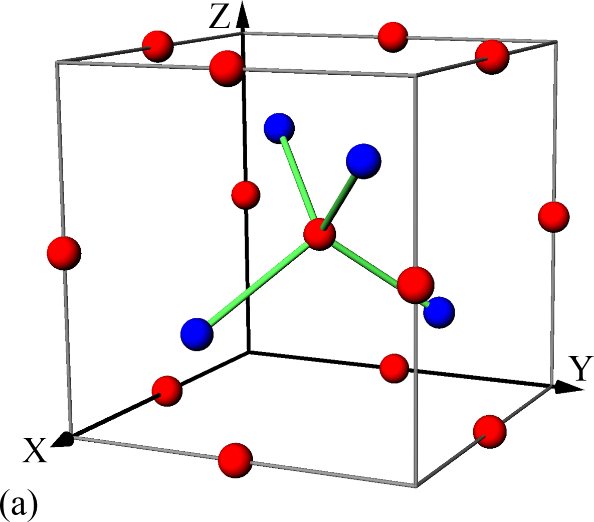
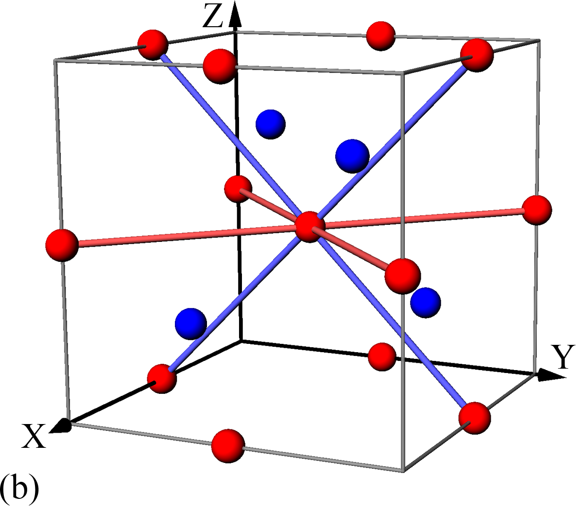
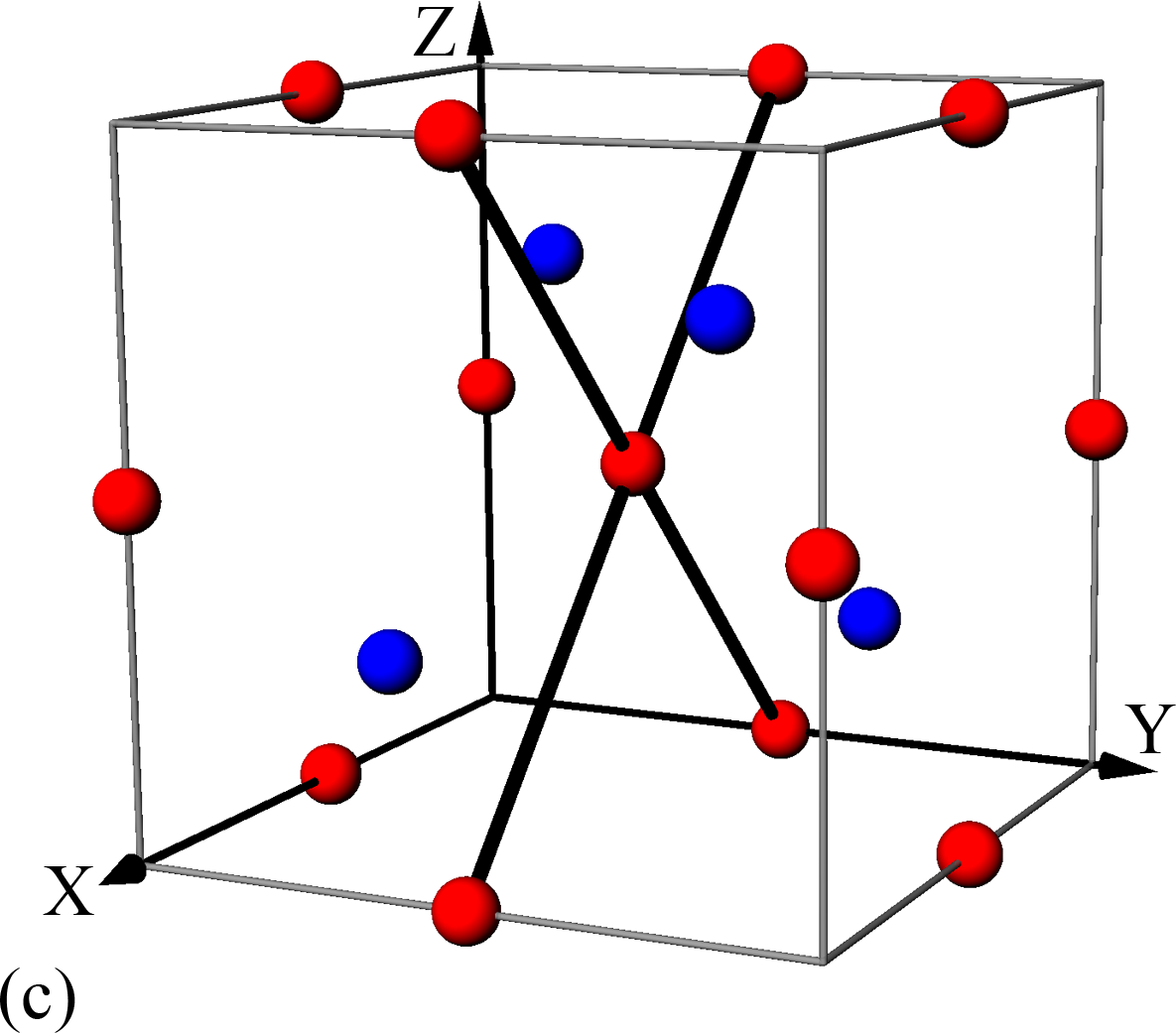
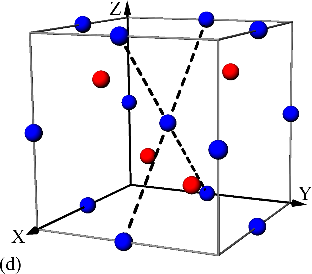
Figure 3: Class AIII model on the diamond lattice. Sublattice A (B) sites are indicated by red (blue) spheres, and are subject to the potential $\mu_{s}$ ($-\mu_{s}$). (a) Nearest-neighbor hopping with amplitude $t^{\prime}$. (b) BCS pairing within each of the sublattices. The red lines indicate $d$-wave spin-singlet pairing in the $xy$ plane. The blue lines indicate $p$-wave $z$-axial spin-triplet pairing in the $yz$ plane. (c) and (d) Next-nearest-neighbor hopping in the $xz$ plane. The solid and dashed lines mean that the hopping amplitudes are $+t$ and $-t$, respectively.

III.1 Topological superconductors on the diamond lattice with spin U(1) symmetry

The Hamiltonian of the topological superconductor model on the diamond lattice consists of three parts,

$$H=H_{\text{nn}}+H_{\text{pair}}+H_{\text{nnn}},$$ (15)

which are defined as the follows.

First, $H_{\text{nn}}$ describes isotropic nearest-neighbor hopping [see Fig. 3(a)],

$$H_{\text{nn}}=t^{\prime}\,\sum_{\mathbf{R}}\sum_{\mu=\uparrow,\downarrow}\sum_{\bm{\delta}\in b_{\text{nn}}}\left[C_{\text{A}\mu}^{\dagger}(\mathbf{R})\,C_{\text{B}\mu}(\mathbf{R}+\bm{\delta})+\text{H.c.}\right],$$ (16)

where $C_{\text{i}\mu}^{\dagger}(\mathbf{R})$ [$C_{\text{i}\mu}(\mathbf{R})$] is the creation (annihilation) operator of a spin $\mu\in\{\uparrow,\downarrow\}$ electron at site $\mathbf{R}$ on the sublattice $\text{i}\in\{\text{A, B}\}$, and $t^{\prime}$ is the hopping strength.

Second, $H_{\text{pair}}$ describes the BCS pairing potentials of electrons within each of the sublattices [see Fig. 3(b)],

$$\begin{split}H_{\text{pair}}=&\frac{1}{2}\sum_{\text{i}=\text{A},\text{B}}\sum_{\mathbf{R}}\sum_{\bm{\delta}\in b_{\text{nnn}}}\sum_{\mu,\nu=\uparrow,\downarrow}\\ &\times\left[\Delta_{\mu\nu}(\bm{\delta})\,C_{\text{i}\mu}^{\dagger}(\mathbf{R})\,C_{\text{i}\nu}^{\dagger}(\mathbf{R}+\bm{\delta})+\text{H.c.}\right].\end{split}$$ (17)

Here the anisotropic pairing amplitudes are encoded in the $2\times 2$ matrices

$$\hat{\Delta}(\bm{\delta})=\begin{cases}i\,\sqrt{3}\,\Delta\,\hat{\mu}^{2}\,\,(\text{d-wave spin-singlet}),&\bm{\delta}\perp\hat{\mathbf{z}},\\ -i\operatorname{sgn}(\delta_{y})\,\Delta\,\hat{\mu}^{1}\,\,(\text{p-wave spin-triplet}),&\bm{\delta}\perp\hat{\mathbf{x}},\\ 0,&\bm{\delta}\perp\hat{\mathbf{y}}.\end{cases}$$ (18)

where $\Delta$ is real and $\hat{\mu}^{\alpha=1,2,3}$ are the set of Pauli matrices acting on the physical spin space. We choose anisotropic pairing potentials in space for the sake of engineering more topologically nontrivial phases.

The last term $H_{\text{nnn}}$ includes a staggered on-site chemical potential and next-nearest-neighbor hopping of electrons [see Figs. 3(c) and 3(d)],

$$\begin{split}H_{\text{nnn}}=&\sum_{\text{i}=\text{A},\text{B}}\sum_{\mathbf{R}}\sum_{\mu=\uparrow,\downarrow}V_{\text{i},s}\,C_{\text{i}\mu}^{\dagger}(\mathbf{R})\,C_{\text{i}\mu}(\mathbf{R})\\ &+\sum_{\text{i}=\text{A},\text{B}}\sum_{\mathbf{R}}\sum_{\bm{\delta}\in b_{\text{nnn}}}\sum_{\mu=\uparrow,\downarrow}\\ &\phantom{++}\times\left[t_{\text{i}}(\bm{\delta})\,C_{\text{i}\mu}^{\dagger}(\mathbf{R})\,C_{\text{i}\mu}(\mathbf{R}+\bm{\delta})+\text{H.c.}\right]\end{split}$$ (19)

where $V_{\text{i},s}=\mu_{s}$ ($-\mu_{s}$) for $\text{i}\in\text{A}$ ($\text{i}\in\text{B}$), and

$$t_{\text{i}}(\bm{\delta})=\begin{cases}t,&\text{i}\in\text{A},\bm{\delta}\perp\hat{\mathbf{y}}\\ -t,&\text{i}\in\text{B},\,\bm{\delta}\perp\hat{\mathbf{y}}\\ 0,&\mbox{otherwise},\end{cases}$$ (20)

with $\mu_{s}$ and $t$ real.

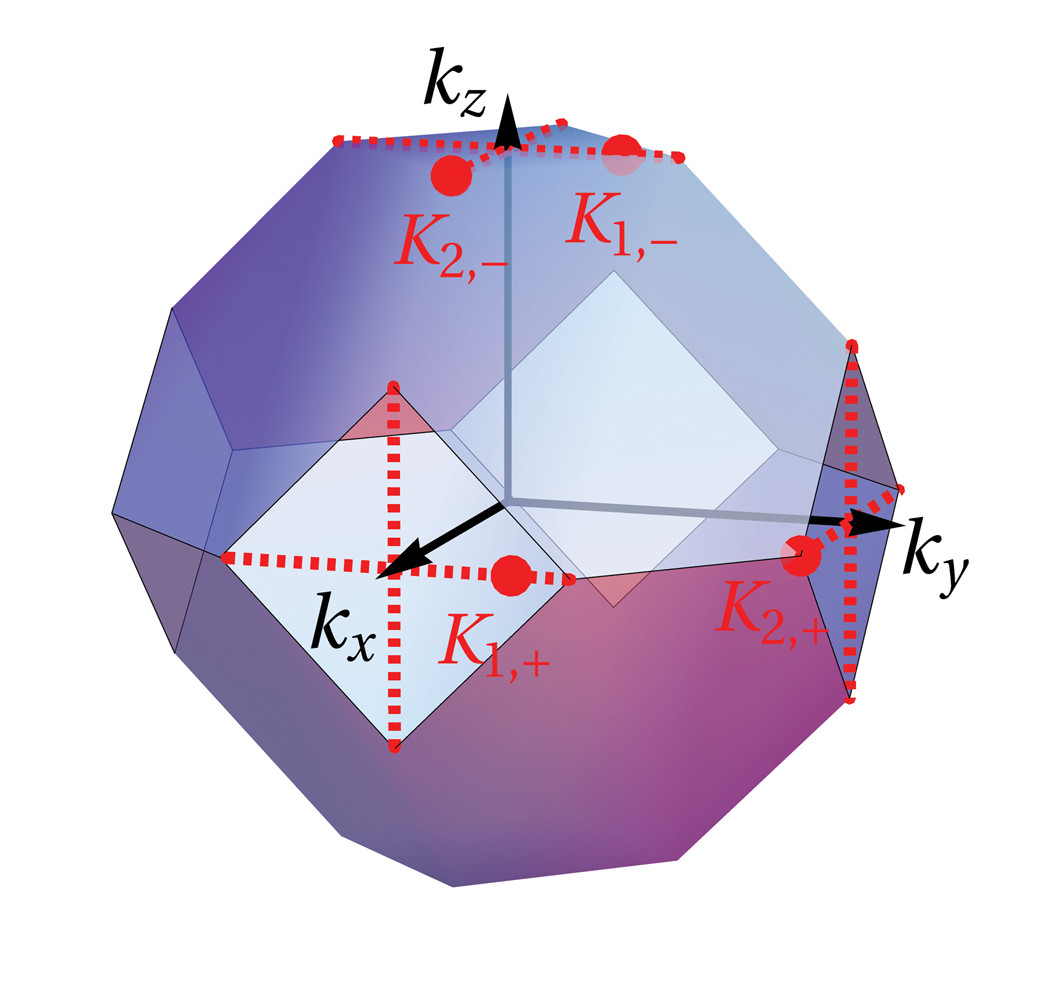
Figure 4: Diagram showing the emergence of the Dirac points of the Hamiltonian (27) in the first Brillouin zone of the diamond lattice, obtained from Eq. (32). The red dashed lines indicate the Fermi surface at half filling when $t=\mu_{s}=\Delta=0$. Nonzero $\Delta$ gaps most of the the Fermi surface except for the massless Dirac nodes indicated by the red spots [Eq. (33)]. Mass gaps open at those Dirac nodes for nonzero $t$ or $\mu_{s}$, so that topologically trivial or nontrivial superconductors can be obtained depending on the values of these. See Fig. 5.

In reciprocal space the Hamiltonian takes the form

$$H=\int\limits_{\text{B.Z.}}\!\frac{\mathrm{d}^{3}{\bf k}}{(2\pi)^{3}}\psi^{\dagger}({\bf k})\,\mathcal{H}({\bf k})\,\psi({\bf k}),$$ (21)

where

$$\psi({\bf k})= \,\begin{bmatrix}C_{\text{A}\uparrow}({\bf k})&C_{\text{B}\uparrow}({\bf k})&C_{\text{A}\downarrow}^{\dagger}(-{\bf k})&C_{\text{B}\downarrow}^{\dagger}(-{\bf k})\end{bmatrix}^{\mathsf{T}}\!\!.$$ (22)

The model is constructed to preserve time-reversal and spin U(1) symmetries. Time-reversal symmetry appears as the antiunitary transformation

$$\begin{gathered}C_{\text{i}\uparrow}({\bf k})\mapsto-C_{\text{i}\downarrow}(-{\bf k}),\quad C_{\text{i}\downarrow}({\bf k})\mapsto C_{\text{i}\uparrow}(-{\bf k}),\\ \psi({\bf k})\mapsto i\,\hat{\sigma}^{2}\,\left[\psi^{\dagger}({\bf k})\right]^{\mathsf{T}},\end{gathered}$$ (25)

where $\hat{\sigma}^{1,2,3}$ is the set of Pauli matrices acting on the particle-hole space. This imposes a chiral condition on the Hamiltonian,

$$-\hat{\sigma}^{2}\,\mathcal{H}({\bf k})\,\hat{\sigma}^{2}=\mathcal{H}({\bf k}).$$ (26)

The conserved U(1) charge of Eq. (21) is the spin projection along the $z$ axis.

Following the analogous construction for class CI SUP-SRL2009 , the Hamiltonian in Eq. (21) is defined as

$$\begin{split}\mathcal{H}({\bf k})=&\,\Theta({\bf k})\,\hat{\sigma}^{3}\otimes\hat{\tau}^{3}+\Delta({\bf k})\,\hat{\sigma}^{1}\\ &\,+\hat{\sigma}^{3}\otimes\left[\Phi_{\text{R}}({\bf k})\,\hat{\tau}^{1}+\Phi_{\text{I}}({\bf k})\,\hat{\tau}^{2}\right],\end{split}$$ (27)

where the Pauli matrices $\hat{\tau}^{1,2,3}$ act on the sublattice space. The potential functions in Eq. (27) are defined as follows. (i) Nearest-neighbor hopping of electrons [Eq. (16)] leads to

$$\begin{aligned} \Phi_{\text{R}}({\bf k})=&4t^{\prime}\cos\left(\frac{k_{x}}{4}\right)\cos\left(\frac{k_{y}}{4}\right)\cos\left(\frac{k_{z}}{4}\right),\\ \Phi_{\text{I}}({\bf k})=&4t^{\prime}\sin\left(\frac{k_{x}}{4}\right)\sin\left(\frac{k_{y}}{4}\right)\sin\left(\frac{k_{z}}{4}\right).\end{aligned}$$ (28)

We consider the case of half-filling, where the Fermi surface is formed by a set of one-dimensional filaments on the diamond faces of the first Brillouin zone. These are depicted as red dashed lines in Fig. 4. (ii) BCS pairing [Eq. (17)] yields

$$\,\Delta({\bf k})=\Delta_{\text{d}}({\bf k})+\Delta_{\text{p}}({\bf k}),$$ (29)

$$\,\begin{aligned} \Delta_{\text{d}}({\bf k})=&\,4\sqrt{3}\,\Delta\,\cos{\left(\frac{k_{x}}{2}\right)}\cos{\left(\frac{k_{y}}{2}\right)},\\ \Delta_{\text{p}}({\bf k})=&\,4\,\Delta\,\sin{\left(\frac{k_{y}}{2}\right)}\cos{\left(\frac{k_{z}}{2}\right)},\end{aligned}$$ (30)

being the Fourier transform of $\hat{\Delta}(\bm{\delta})$ in Eq. (18). The p-wave pairing $\Delta_{\text{p}}({\bf k})$ breaks the spin SU(2) symmetry down to the subgroup of U(1) rotations about the $z$ axis, but preserves time-reversal symmetry (class AIII). These pairing potentials gap out most of the Fermi surface, leaving four isolated Dirac nodal points denoted by the red spots in Fig. 4. (iii) Staggered on-site chemical potential and next-nearest-neighbor hopping [Eq. (19)] give

$$\Theta({\bf k})=4\,t\,\cos{\left(\frac{k_{x}}{2}\right)}\cos{\left(\frac{k_{z}}{2}\right)}+\mu_{s}.$$ (31)

Nonzero $\mu_{s}$ or $t$ opens mass gaps at the Dirac nodes. The gapped phase can be a trivial or topological superconductor.

The energy eigenvalues of $\mathcal{H}({\bf k})$ are

$$E_{\pm}({\bf k})=\pm\sqrt{\Theta^{2}({\bf k})+\Delta^{2}({\bf k})+\Phi_{\text{R}}^{2}({\bf k})+\Phi_{\text{I}}^{2}({\bf k})},$$ (32)

with a twofold degeneracy for each momentum ${\bf k}$. For $t=\mu_{s}=0$ and nonzero $t^{\prime}$ and $\Delta$, there are four massless Dirac nodes at

$$\begin{split}\mathbf{K}_{1,+}=&\,2\pi\,(1,1/3,0),\quad\mathbf{K}_{1,-}=2\pi\,(0,1/3,1),\\ \mathbf{K}_{2,+}=&\,2\pi\,(1/2,1,0),\quad\mathbf{K}_{2,-}=2\pi\,(1/2,0,1),\end{split}$$ (33)

as shown in Fig. 4. For nonzero $t$ and $\mu_{s}$, the Dirac masses at these nodes are

$$\mathbf{K}_{1,\pm}\!:\;M_{1}\equiv\mu_{s}-4t,\;\;\mathbf{K}_{2,\pm}\!:\;M_{2}\equiv\mu_{s}.$$ (34)

Thus gapless bulk quasiparticles survive for $\mu_{s}=4t$ and $\mu_{s}=0$. When crossing one of these cut lines in the $t$-$\mu_{s}$ plane, the energy gap closes and reopens, potentially signaling a topological phase transition.

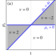
Figure 5: Topological superconducting phases of Eq. (21) as a function of the next-nearest-neighbor hopping strength $t$ and the staggered chemical potential $\mu_{s}$. (a) Phase diagram. The blue lines indicate the phase boundaries where the bulk gap closes. The gray area indicates the topologically nontrivial phases with $|\nu|=2$, where the superconductor possesses two gapless surface bands. (b) Numerical results for the winding number [Eq. (37)], with $\Delta=2$ and $t^{\prime}=4$.

After a particle-hole space rotation such that $(\hat{\sigma}^{1},\,\hat{\sigma}^{2},\,\hat{\sigma}^{3})\to(\hat{\sigma}^{1},\,-\hat{\sigma}^{3},\,\hat{\sigma}^{2})$, $\mathcal{H}({\bf k})$ takes the off-diagonal form

$$\mathcal{H}({\bf k})\to\begin{pmatrix}0&\hat{D}({\bf k})\\ \hat{D}^{\dagger}({\bf k})&0\end{pmatrix},$$

$$\hat{D}({\bf k})=\Delta({\bf k})-i\,\Phi_{\text{R}}({\bf k})\,\hat{\tau}^{1}-i\,\Phi_{\text{I}}({\bf k})\,\hat{\tau}^{2}-i\,\,\Theta({\bf k})\,\hat{\tau}^{3}.$$ (35)

One then introduces the unitary matrix

$$\hat{q}({\bf k})=-\hat{D}({\bf k})/E_{+}({\bf k}),$$ (36)

with $E_{+}({\bf k})$ defined in Eq. (32). The integer-valued winding number is SRFL2008

$$\nu[\hat{q}]=\int\limits_{\text{B.Z.}}\!\frac{\mathrm{d}^{3}{\bf k}}{24\pi^{2}}\varepsilon^{\alpha\beta\gamma}\text{Tr}\left[(\hat{q}^{-1}\partial_{\alpha}\hat{q})(\hat{q}^{-1}\partial_{\beta}\hat{q})(\hat{q}^{-1}\partial_{\gamma}\hat{q})\right].$$ (37)

The phase diagram is shown in Fig. 5, where the gray regions indicate nontrivial phases with $\nu=\pm 2$ (two surface colors).

In order to produce richer topological phases, one can choose a different type of BCS pairing and next-nearest-neighbor hopping, for example,

$$\hat{\Delta}(\bm{\delta})=\begin{cases}i\,\sqrt{3}\,\Delta\,\hat{\mu}^{2}\,\,(\text{d-wave spin-singlet}),&\bm{\delta}\perp\hat{\mathbf{z}},\\ -i\operatorname{sgn}(\delta_{y})\,\Delta\,\hat{\mu}^{1}\,\,(\text{p-wave spin-triplet}),&\bm{\delta}\perp\hat{\mathbf{x}}\\ -i\operatorname{sgn}(\delta_{x})\,\Delta\,\hat{\mu}^{1}\,\,(\text{p-wave spin-triplet}),&\bm{\delta}\perp\hat{\mathbf{y}},\end{cases}$$ (38)

and

$$t_{\text{i}}(\bm{\delta})=\begin{cases}t/2,&\text{i}\in\text{A},\bm{\delta}\perp\hat{\mathbf{y}},\text{or},\,\text{i}\in B,\,\bm{\delta}\perp\hat{\mathbf{x}}\\ -t/2,&\text{i}\in\text{A},\,\bm{\delta}\perp\hat{\mathbf{x}},\,\text{or},\,\text{i}\in\text{B},\,\bm{\delta}\perp\hat{\mathbf{y}}\\ 0,&\bm{\delta}\perp\hat{\mathbf{z}}.\end{cases}$$ (39)

The corresponding potential functions in momentum space are

$$\begin{aligned} \Delta_{\text{d}}({\bf k})=&4\sqrt{3}\,\Delta\,\cos{\left(\frac{k_{x}}{2}\right)}\cos{\left(\frac{k_{y}}{2}\right)},\\ \Delta_{\text{p}}({\bf k})=&4\,\Delta\,\left[\sin{\left(\frac{k_{x}}{2}\right)}+\sin{\left(\frac{k_{y}}{2}\right)}\right]\cos{\left(\frac{k_{z}}{2}\right)}.\end{aligned}$$ (40)

and

$$\Theta({\bf k})=2\,t\,\left[\cos{\left(\frac{k_{x}}{2}\right)}-\cos{\left(\frac{k_{y}}{2}\right)}\right]\cos{\left(\frac{k_{z}}{2}\right)}+\mu_{s}.$$ (41)

Substituting Eqs. (40) and (41) together with Eq. (28) into Eqs. (27) and (32), and evaluating winding number by Eq. (37), we obtain the phase diagram shown in Fig. 6. In addition to the topological phase with winding number $|\nu|=2$, we obtain the phase with $|\nu|=1$.

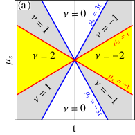
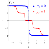
Figure 6: Topological phases of the BCS Hamiltonian (21) with pairing potential in Eq. (40) and next-nearest-neighbor hopping in Eq. (41). (a) Phase diagram. The blue and red lines indicate the phase boundaries where the bulk gap closes. The gray and yellow areas indicate the topological phase with $|\nu|=1$ (one surface color) and $|\nu|=2$ (two surface colors), respectively. (b) Numerical results of the winding number [Eq. (37)] for $\Delta=2$ and $t^{\prime}=4$.

III.2 Low-energy surface state theory

A low-energy field theory can be obtained by expanding $\mathcal{H}({\bf k})$ in Eq. (27) around the four Dirac nodes in Eq. (33), when $\mu_{s}$ and $t$ are small compared to $t^{\prime}$ and $\Delta$. This incorporates two independent pairs of 3D mass-degenerate Dirac fermions, with masses given by Eq. (34). To obtain an effective theory for the surface states, we allow the Dirac masses to vary with some spatial coordinate, say, the $z$ direction. We consider

$$M_{1}=M_{1}(z)=M_{0}\,\text{sgn}(z),\quad M_{2}=\text{Const.}$$ (42)

More generally, $M_{2}$ is allowed to vary along $z$ as long as its sign remains fixed. The phase diagram shown in Fig. 5(a) implies that the phase with $z>0$ is a topological trivial superconductor, while $z<0$ is nontrivial. Since $|M_{2}|\neq 0$ everywhere in space, the Dirac fermions located at $\mathbf{K}_{2,\pm}$ are gapped and can be neglected.

In real space, the bulk low-energy Dirac theory arising from the nodes $\mathbf{K}_{1,\pm}$ can be expressed as

$$H_{D}=\int_{\mathbf{r},z}\!\Psi^{\dagger}(\mathbf{r},z)\,\mathcal{H}_{D}(\mathbf{r},z)\,\Psi(\mathbf{r},z),$$ (43)

where $\mathbf{r}$ is the 2D coordinate on the interface $z=0$, $\int_{\mathbf{r},z}$ denotes the spatial integration $\int\!\mathrm{d}^{2}\mathbf{r}\mathrm{d}z$, and $\Psi(\mathbf{r},z)$ is an eight-component spinor, a direct product of particle-hole, sublattice, and node (“color”) $\mathbf{K}_{1,\pm}$ degrees of freedom. After performing a unitary transformation and rescaling to eliminate velocity anisotropies, the Dirac Hamiltonian is

$$\mathcal{H}_{D}(\mathbf{r},z)=-i\hat{\bm{\sigma}}\cdot\bm{\nabla}-i\,\hat{\sigma}^{3}\otimes\hat{\tau}^{2}\,\partial_{z}+M_{1}(z)\,\hat{\sigma}^{3}\otimes\hat{\tau}^{3}.$$ (44)

The chiral symmetry (26) is brought to the form

$$-(\hat{\sigma}^{3}\otimes\hat{\tau}^{1})\mathcal{H}_{D}(\hat{\sigma}^{3}\otimes\hat{\tau}^{1})=\mathcal{H}_{D}.$$ (45)

The spinor $\Psi(\mathbf{r},z)$ can be decomposed into surface and bulk parts SUP-JR1976 ,

$$\Psi(\mathbf{r},z)=\begin{bmatrix}\eta(\mathbf{r})\\ -\eta(\mathbf{r})\end{bmatrix}\sqrt{\frac{M_{0}}{2}}e^{-M_{0}|z|}+\text{bulk states},$$ (46)

where $\Psi(\mathbf{r},z)$ is explicitly graded by $\hat{\tau}^{3}$. Inserting Eq. (46) into Eq. (43), disregarding the contribution of the bulk states, and integrating over $z$, we finally obtain the 2D Dirac Hamiltonian describing the surface states:

$$H_{\text{surf.}}=\int_{\mathbf{r}}\eta^{\dagger}(\mathbf{r})\,\hat{h}\,\eta(\mathbf{r}),\;\;\hat{h}=-i\,\hat{\bm{\sigma}}\cdot\bm{\nabla}.$$ (47)

At the surface, the physical time-reversal symmetry encoded in the chiral condition (26) assumes the form in Eq. (5), which is the projection of Eq. (45) to the subspace $\hat{\tau}^{1}=-1$ [Eq. (46)]. Equation (5) prohibits a surface Dirac mass term $m=\eta^{\dagger}\hat{\sigma}^{3}\eta$. Weak interactions cannot open a gap unless time-reversal symmetry is broken, either spontaneously or by external means.

IV Kubo formalism for spin conductivity

In this section we compute the interaction corrections to the surface state dc spin conductivity in a disordered class CI or AIII TSC, at zero temperature. Class CI preserves spin SU(2) in every disorder realization, while class AIII preserves the spin-$z$ component SRFL2008 ; FXCup . We evaluate the Kubo formula for the conserved $z$-spin current $\mathbf{J}^{z}$ defined in Eq. (4). We show that quantum conductance corrections due to short-ranged interactions vanish. These results hold in every fixed realization of the disorder, including the clean limit, and are obtained without detailed knowledge of the noninteracting Green’s functions. Instead, we exploit only general properties such as the Ward identity and the chiral symmetry in Eq. (7) of the main text. We explicitly evaluate corrections to first (second) order in the interaction strengths for class CI (AIII). We also sketch a proof for the cancellation of corrections to all orders for class AIII.

The Kubo formula for the dc spin conductivity is SUP-mahanbook

$$\sigma_{\mathrm{s}}^{\alpha\beta}=\lim_{\omega\to 0}\,{\frac{1}{\omega\mathcal{V}}\,\text{Im}\left\{\Pi_{\alpha\beta}(i\Omega_{n})|_{i\Omega_{n}\to\omega+i\delta}\right\}},$$ (48)

where $\mathcal{V}$ is the system volume and the current-current correlation function is defined by

$$\Pi_{\alpha\beta}(i\Omega_{n})=\int_{0}^{1/T}\!d\tau\,e^{i\Omega_{n}\tau}\,\left\langle\mathbf{T_{\tau}}\,j_{\alpha}(\tau)\,j_{\beta}(0)\right\rangle.$$ (49)

Here $\alpha,\beta=1,2$ are directions in real space, $T$ is the temperature, $j_{\alpha}(\tau)$ is the current operator at imaginary time $\tau$, and the bracket $\langle\cdots\rangle$ denotes the thermal average. The spin-$z$ current operator is [see Eq. (4)]

$$j_{\alpha}(\tau)=\int_{\mathbf{r}}\eta^{\dagger}(\mathbf{r},\tau)\,\hat{\sigma}^{\alpha}\,\eta(\mathbf{r},\tau),\quad\alpha\in\{1,2\}.$$ (50)

In the absence of interactions and the presence of nonmagnetic disorder, the Hamiltonian is given by Eq. (3).

We represent the exact noninteracting single-particle retarded and advanced Green’s functions by matrices whose elements are defined by

$$\left[\hat{G}_{12}^{R/A}({\epsilon})\right]_{ab}\equiv\sum_{j}{\frac{\varphi_{j}(a,\mathbf{r}_{1})\,\varphi_{j}^{\ast}(b,\mathbf{r}_{2})}{{\epsilon}-{\epsilon}_{j}\pm i\delta}},$$ (51)

where $a,b$ are shorthand indices for the pseudospin and color degrees of freedom, and $j$ labels the exact single-particle wave function at an eigenenergy ${\epsilon}_{j}$. Apart from the general relation

$$\left[\hat{G}_{12}^{R/A}({\epsilon})\right]^{\dagger}=\hat{G}_{21}^{A/R}({\epsilon}),$$ (52)

time-reversal symmetry [Eq. (5)] allows one to relate the two types of Green’s functions via Eq. (7). The Matsubara Green’s function satisfies

$$-\hat{\sigma}^{3}\,\hat{G}_{12}(i\omega_{n})\,\hat{\sigma}^{3}=\hat{G}_{12}(-i\omega_{n}).$$ (53)

In what follows we will exploit the Ward identities mirlin2006 ; SUP-mahan2 ,

$$\int_{\mathbf{r}_{3}}\hat{G}_{13}^{R/A}({\epsilon})\,\hat{\sigma}^{\alpha}\,\hat{G}_{32}^{R/A}({\epsilon})=-i\,(\mathbf{r}_{1}-\mathbf{r}_{2})^{\alpha}\,\hat{G}_{12}^{R/A}({\epsilon}),$$ (54a)

$$\int_{\mathbf{r}_{3}}\hat{G}_{13}(i\omega_{n})\,\hat{\sigma}^{\alpha}\,\hat{G}_{32}(i\omega_{n})=-i\,(\mathbf{r}_{1}\!-\!\mathbf{r}_{2})^{\alpha}\,\hat{G}_{12}(i\omega_{n}),$$ (54b)

and the following relations between the components of the spin U(1) current operator in Eq. (50):

$$-\hat{\sigma}^{3}\,\hat{\sigma}^{\alpha}\,\hat{\sigma}^{3}=\hat{\sigma}^{\alpha},\;\;\hat{\sigma}^{3}\hat{\sigma}^{\alpha}=i\,\varepsilon_{\alpha\beta}\,\hat{\sigma}^{\beta},$$ (55)

where $\varepsilon_{\alpha\beta}$ is the 2D Levi-Civita symbol.

We consider squared $z$-spin $(S^{z})^{2}$ and Dirac mass $m^{2}$ interactions, as appear in Eq. (6) for class AIII. For class CI, the Hartree and Fock corrections will be the same for $(S^{\alpha})^{2}$ ($\alpha\in\{x,y,z\}$) interactions, by SU(2) symmetry. The $z$-spin density and Dirac mass (Cooper pair density Foster2012 ; FXCup ) operators are

$$S^{z}(\mathbf{r})=\eta^{\dagger}\,\eta(\mathbf{r}),\quad m(\mathbf{r})=\eta^{\dagger}\,\hat{\sigma}^{3}\,\eta(\mathbf{r}).$$ (56)

We define

$$\hat{s}\in\left\{\hat{1},\hat{\sigma}^{3}\right\},$$ (57)

so that both are encoded as $\eta^{\dagger}\hat{s}\eta$.

IV.1 Hartree-Fock spin conductivity

The lowest-order diagrams for the interaction correction to Eq. (49), which is denoted by $\delta\Pi_{\alpha\beta}^{(1)}$, are shown in Fig. 2, where (a) corresponds to the Hartree diagrams and (b) to the Fock ones. The Hartree diagrams give

$$\delta\Pi_{\alpha\beta}^{(1a)}(i\Omega_{n})=-\Gamma_{\mathrm{s},\mathrm{c}}\,(-1)^{2}\,T^{2}\sum_{i\omega_{p},i\omega_{q}}\;\int_{\mathbf{r}_{1},\mathbf{r}_{2},\mathbf{r}_{3}}$$

$$\times\!\!\left\{\text{Tr}\left[\hat{\sigma}^{\alpha}\,\hat{G}_{12}(i\omega_{p})\,\hat{\sigma}^{\beta}\,\hat{G}_{23}(i\omega_{p}+i\Omega_{n})\,\hat{s}\,\hat{G}_{31}(i\omega_{p}+i\Omega_{n})\right]\right.$$

$$\phantom{+}\qquad\left.\times\text{Tr}\left[\hat{s}\,\hat{G}_{33}(i\omega_{q})\right]\right.$$ (58a)

$$\phantom{+}\left.+\text{Tr}\left[\hat{\sigma}^{\beta}\,\hat{G}_{21}(i\omega_{p})\,\hat{\sigma}^{\alpha}\,\hat{G}_{13}(i\omega_{p}-i\Omega_{n})\,\hat{s}\,\hat{G}_{32}(i\omega_{p}-i\Omega_{n})\right]\right.$$

$$\phantom{+}\qquad\left.\times\text{Tr}\left[\hat{s}\,\hat{G}_{33}(i\omega_{q})\right]\right.$$ (58b)

$$\phantom{+}\left.+\text{Tr}\left[\hat{s}\,\hat{G}_{31}(i\omega_{p})\,\hat{\sigma}^{\alpha}\,\hat{G}_{13}(i\omega_{p}-i\Omega_{n})\right]\right.$$

$$\phantom{+}\qquad\left.\times\text{Tr}\left[\hat{s}\,\hat{G}_{32}(i\omega_{q})\,\hat{\sigma}^{\beta}\,\hat{G}_{23}(i\omega_{q}+i\Omega_{n})\right]\right\},\!\!\!$$ (58c)

where the terms (58a)-(58c) come from the diagrams a(i)-a(iii), respectively. The Fock diagrams give

$$\delta\Pi_{\alpha\beta}^{(1b)}(i\Omega_{n})=-\Gamma_{\mathrm{s},\mathrm{c}} \,(-1)\,T^{2}\sum_{i\omega_{p},i\omega_{q}}\;\int_{\mathbf{r}_{1},\mathbf{r}_{2},\mathbf{r}_{3}}$$

$$\,\times\left\{\text{Tr}\left[\hat{\sigma}^{\alpha}\,\hat{G}_{12}(i\omega_{p}\!\!\right.\right. \left.\left.\!\!)\,\hat{\sigma}^{\beta}\,\hat{G}_{23}(i\omega_{p}+i\Omega_{n})\,\hat{s}\,\hat{G}_{33}(i\omega_{q})\,\right.\right.$$

$$\!\!\!\!\!\!\!\!\!\!\!\!\!\!\!\!\!\!\!\!\!\!\!\!\!\!\!\!\!\!\!\!\left.\left.\times\hat{s}\,\hat{G}_{31}(i\omega_{p}+i\Omega_{n})\,\right]\right.$$ (59a)

$$\left.+\text{Tr}\left[\hat{\sigma}^{\beta}\,\hat{G}_{21}(i\omega_{p}\!\!\right.\right. \left.\left.\!\!)\,\hat{\sigma}^{\alpha}\,\hat{G}_{13}(i\omega_{p}-i\Omega_{n})\,\hat{s}\,\hat{G}_{33}(i\omega_{q})\,\right.\right.$$

$$\!\!\!\!\!\!\!\!\!\!\!\!\!\!\!\!\!\!\!\!\!\!\!\!\!\!\!\!\!\!\!\!\left.\left.\times\hat{s}\,\hat{G}_{32}(i\omega_{p}-i\Omega_{n})\,\right]\right.$$ (59b)

$$\left.+\text{Tr}\left[\hat{s}\,\hat{G}_{31}(i\omega_{p})\,\!\!\right.\right. \left.\left.\!\!\hat{\sigma}^{\alpha}\,\hat{G}_{13}(i\omega_{p}-i\Omega_{n})\,\hat{s}\,\hat{G}_{32}(i\omega_{q})\,\right.\right.$$

$$\!\!\!\!\!\!\!\!\!\!\!\!\!\!\!\!\!\!\!\!\!\!\!\!\!\!\!\!\!\!\!\!\left.\left.\times\hat{\sigma}^{\beta}\,\hat{G}_{23}(i\omega_{q}+i\Omega_{n})\right]\right\},$$ (59c)

where (59a)-(59c) come from the diagrams b(i)-b(iii), respectively.

The Hartree terms (58a) and (58b) vanish individually, due to Eq. (53) and the fact that $[\hat{s},\hat{\sigma}^{3}]=0$. The Fock terms (59a) and (59b) give the same contribution. Equations (58c) and (59c) do not contribute to the dc conductivity, because they are of the order of $\Omega^{2}$ when $\Omega\to 0$. Therefore, we only have to further analyze the contributions of Eqs. (59a) and (59b):

$$\delta\Pi_{\alpha\alpha}^{(1b)} (i\Omega_{n})=2\,\Gamma_{\mathrm{s},\mathrm{c}}\,T\sum_{i\omega_{p}}\;\int_{\mathbf{r}_{1},\mathbf{r}_{2},\mathbf{r}_{3}}\text{Tr}\left[\hat{s}\,\hat{\rho}_{3}\,\hat{s}\,\right.$$

$$\times \left.\hat{G}_{31}(i\omega_{p}-i\Omega_{n})\,\hat{\sigma}^{\alpha}\,\hat{G}_{12}(i\omega_{p})\,\hat{\sigma}^{\alpha}\,\hat{G}_{23}(i\omega_{p}-i\Omega_{n})\right].$$ (60)

Here we have defined the local $z$-spin density matrix

$$\begin{split}\left(\hat{\rho}_{3}\right)_{ab}&\equiv T\sum_{i\omega_{q}}\left[\hat{G}_{33}(i\omega_{q})\right]_{ab}\\ &=\sum_{j}{\varphi_{j}(a,\mathbf{r}_{3})\,\varphi_{j}^{\ast}(b,\mathbf{r}_{3})}f({\epsilon}_{j}),\end{split}$$ (61)

where $f({\epsilon}_{j})$ is the Fermi-Dirac distribution function. One can easily prove that $-\hat{\sigma}^{3}\,\hat{\rho}_{3}\,\hat{\sigma}^{3}=\hat{\rho}_{3}$. Applying the standard analytic continuation technique SUP-mahanbook we obtain

$$\begin{split}\delta&\Pi_{\alpha\alpha}^{(1b)}(\omega)=-2\Gamma_{\mathrm{s},\mathrm{c}}\int_{-\infty}^{+\infty}\frac{d{\epsilon}}{2\pi i}\;\int_{\mathbf{r}_{1},\mathbf{r}_{2},\mathbf{r}_{3}}\text{Tr}\bigg{[}\hat{s}\,\hat{\rho}_{3}\,\hat{s}\\ &\times\left.\left\{\left[f({\epsilon}+\omega)-f({\epsilon})\right]\,\hat{G}_{31}^{A}({\epsilon})\,\hat{\sigma}^{\alpha}\,\hat{G}_{12}^{R}({\epsilon}+\omega)\,\hat{\sigma}^{\alpha}\,\hat{G}_{23}^{A}({\epsilon})\right.\right.\\ &\left.\left.\qquad+f({\epsilon})\,\hat{G}_{31}^{R}({\epsilon})\,\hat{\sigma}^{\alpha}\,\hat{G}_{12}^{R}({\epsilon}+\omega)\,\hat{\sigma}^{\alpha}\,\hat{G}_{23}^{R}({\epsilon})\right.\right.\\ &\left.\qquad-f({\epsilon}+\omega)\,\hat{G}_{31}^{A}({\epsilon})\,\hat{\sigma}^{\alpha}\,\hat{G}_{12}^{A}({\epsilon}+\omega)\,\hat{\sigma}^{\alpha}\,\hat{G}_{23}^{A}({\epsilon})\right\}\bigg{]}.\end{split}$$ (62)

Therefore, the correction to Eq. (1) reads

$$\delta\sigma_{\mathrm{s}}^{\alpha\alpha}= \frac{1}{\mathcal{V}}\lim_{\omega\to 0}\frac{1}{2i\omega}\left[\delta\Pi_{\alpha\alpha}^{(1b)}(\omega)-\delta{\Pi_{\alpha\alpha}^{(1b)}}^{\ast}(\omega)\right]$$

$$= \frac{\Gamma_{\mathrm{s},\mathrm{c}}}{2\pi\mathcal{V}}\int_{-\infty}^{+\infty}\!d{\epsilon}\,\frac{df({\epsilon})}{d{\epsilon}}\,\;\int_{\mathbf{r}_{1},\mathbf{r}_{2},\mathbf{r}_{3}}\text{Tr}\left\{\hat{s}\,\hat{\rho}_{3}\,\hat{s}\right.$$

$$\times\left.\left[\hat{G}_{31}^{A}({\epsilon})\,\hat{\sigma}^{\alpha}\,\hat{G}_{12}^{R}({\epsilon})\,\hat{\sigma}^{\alpha}\,\hat{G}_{23}^{A}({\epsilon})\right.\right.$$

$$\left.\left.\quad\,+\hat{G}_{31}^{R}({\epsilon})\,\hat{\sigma}^{\alpha}\,\hat{G}_{12}^{A}({\epsilon})\,\hat{\sigma}^{\alpha}\,\hat{G}_{23}^{R}({\epsilon})\right.\right.$$

$$\left.\left.\quad\,-\hat{G}_{31}^{R}({\epsilon})\,\hat{\sigma}^{\alpha}\,\hat{G}_{12}^{R}({\epsilon})\,\hat{\sigma}^{\alpha}\,\hat{G}_{23}^{R}({\epsilon})\right.\right.$$

$$\left.\left.\quad\,-\hat{G}_{31}^{A}({\epsilon})\,\hat{\sigma}^{\alpha}\,\hat{G}_{12}^{A}({\epsilon})\,\hat{\sigma}^{\alpha}\,\hat{G}_{23}^{A}({\epsilon})\right]\right\},$$ (63)

where we have used Eq. (52).

At zero temperature, Eq. (IV.1) can be expressed entirely in terms of retarded Green’s functions,

$$\delta\sigma_{\mathrm{s}}^{\alpha\alpha}= -\frac{\Gamma_{\mathrm{s},\mathrm{c}}}{2\pi\mathcal{V}}\sum_{\beta=1}^{2}\int_{\mathbf{r}_{1},\mathbf{r}_{2},\mathbf{r}_{3}}\text{Tr}\Big{[}\left(\hat{\sigma}^{3}\hat{\rho}_{3}\hat{\sigma}^{3}-\hat{\rho}_{3}\right)$$

$$\qquad\quad\times\hat{s}\,\hat{G}_{31}^{R}(0)\,\hat{\sigma}^{\beta}\,\hat{G}_{12}^{R}(0)\,\hat{\sigma}^{\beta}\,\hat{G}_{23}^{R}(0)\hat{s}\Big{]}.$$ (64)

To derive this, we replace all advanced Green’s functions with retarded ones using Eq. (7), and employ Eq. (55). Finally, we use the Ward identity (54a) to show that this expression is zero. Integrating over $\mathbf{r}_{1}$ yields

$$\delta\sigma_{\mathrm{s}}^{\alpha\alpha}= \,i\frac{\Gamma_{\mathrm{s},\mathrm{c}}}{2\pi\mathcal{V}}\sum_{\beta=1}^{2}\int_{\mathbf{r}_{2},\mathbf{r}_{3}}(\mathbf{r}_{3}-\mathbf{r}_{2})^{\beta}$$

$$\times \text{Tr}\Big{[}\left(\hat{\sigma}^{3}\hat{\rho}_{3}\hat{\sigma}^{3}-\hat{\rho}_{3}\right)\hat{s}\hat{G}_{32}^{R}(0)\,\hat{\sigma}^{\beta}\,\hat{G}_{23}^{R}(0)\hat{s}\Big{]}.$$ (65)

Integrating over $\mathbf{r}_{2}$ instead gives

$$\delta\sigma_{\mathrm{s}}^{\alpha\alpha}= i\frac{\Gamma_{\mathrm{s},\mathrm{c}}}{2\pi\mathcal{V}}\sum_{\beta=1}^{2}\int_{\mathbf{r}_{1},\mathbf{r}_{3}}(\mathbf{r}_{1}-\mathbf{r}_{3})^{\beta}$$

$$\times \text{Tr}\Big{[}\left(\hat{\sigma}^{3}\hat{\rho}_{3}\hat{\sigma}^{3}-\hat{\rho}_{3}\right)\hat{s}\hat{G}_{31}^{R}(0)\,\hat{\sigma}^{\beta}\,\hat{G}_{13}^{R}(0)\hat{s}\Big{]}$$

$$= -\delta\sigma_{\mathrm{s}}^{\alpha\alpha}.$$ (66)

The Hartree and Fock corrections vanish for both spin- and mass-squared interactions.

IV.2 Second-order corrections

The second-order interaction corrections to the spin conductivity in class AIII are represented by the Feynman diagrams in Fig. 7. Clearly the diagrams including at least one Hartree bubble, for example, a(i) and a(ii), are individually zero due to the chiral condition (53). The diagrams a(iii)–a(v) do not contribute to the dc conductivity because they are of the order of $\Omega^{2}$ when $\Omega\to 0$. Moreover, comparing a(vi) to Fig. 2(b)(i) one can readily prove that the dc conductivity correction arising from a(vi) vanishes at zero temperature. Here we show that the diagrams in each category (b)–(f) depicted in Fig. 7 altogether give null contribution.

Figure 7: The second-order interaction corrections to the spin current-current correlation function in class AIII. The Feynman rules are interpreted in the caption for Fig. 2 of the main text.

IV.2.1 Category b

The current-current correlation functions represented by b(i) and b(ii) read

$$\delta\Pi_{\alpha\alpha}^{[\mathrm{b(i)}]}(i\Omega_{n})=-\Gamma_{\mathrm{s},\mathrm{c}}^{2}\,T\sum_{i\omega_{p}}\int_{\mathbf{r}_{1},\mathbf{r}_{2},\mathbf{r}_{3},\mathbf{r}_{4}}$$

$$\times\text{Tr}\left[\hat{G}_{41}(i\omega_{p}+i\Omega_{n})\,\hat{\sigma}^{\alpha}\,\hat{G}_{12}(i\omega_{p})\,\hat{\sigma}^{\alpha}\,\hat{G}_{23}(i\omega_{p}+i\Omega_{n})\right.$$

$$\left.\hskip 22.76228pt\times\,\hat{s}\,\hat{\rho}_{3}\,\hat{s}\,\hat{G}_{34}(i\omega_{p}+i\Omega_{n})\hat{s}\,\hat{\rho}_{4}\,\hat{s}\,\right],$$ (67a)

$$\delta\Pi_{\alpha\alpha}^{[\mathrm{b(ii)}]}(i\Omega_{n})=-\Gamma_{\mathrm{s},\mathrm{c}}^{2}\,T\sum_{i\omega_{p}}\int_{\mathbf{r}_{1},\mathbf{r}_{2},\mathbf{r}_{3},\mathbf{r}_{4}}$$

$$\times\text{Tr}\left[\hat{G}_{41}(i\omega_{p}+i\Omega_{n})\,\hat{\sigma}^{\alpha}\hat{G}_{13}(i\omega_{p})\,\hat{s}\,\hat{\rho}_{3}\,\hat{s}\,\hat{G}_{32}(i\omega_{p})\right.$$

$$\left.\hskip 22.76228pt\times\,\hat{\sigma}^{\alpha}\,\hat{G}_{24}(i\omega_{p}+i\Omega_{n})\hat{s}\,\hat{\rho}_{4}\,\hat{s}\right],$$ (67b)

where the local $z$-spin density matrix $\hat{\rho}_{3}$ is defined in Eq. (61). After analytic continuation we obtain

$$\delta\Pi_{\alpha\alpha}^{[\mathrm{b(i)}]}(\omega)=\Gamma_{\mathrm{s,c}}^{2}\,\int_{-\infty}^{+\infty}\frac{\mathrm{d}{\epsilon}}{2\pi i}\int_{\mathbf{r}_{1},\mathbf{r}_{2},\mathbf{r}_{3},\mathbf{r}_{4}}$$

$$\times\text{Tr}\left\{[f({\epsilon})-f({\epsilon}-\omega)]\,\hat{\sigma}^{\alpha}\hat{G}_{12}^{A}({\epsilon}-\omega)\,\hat{\sigma}^{\alpha}\,\hat{G}_{23}^{R}({\epsilon})\hat{s}\,\hat{\rho}_{3}\,\hat{s}\right.$$

$$\hskip 22.76228pt\times\left.\hat{G}_{34}^{R}({\epsilon})\hat{s}\hat{\rho}_{4}\,\hat{s}\,\hat{G}_{41}^{R}({\epsilon})+f({\epsilon}-\omega)\,\hat{\sigma}^{\alpha}\hat{G}_{12}^{R}({\epsilon}-\omega)\,\right.$$

$$\hskip 22.76228pt\times\hat{\sigma}^{\alpha}\,\hat{G}_{23}^{R}({\epsilon})\hat{s}\,\hat{\rho}_{3}\,\hat{s}\,\hat{G}_{34}^{R}({\epsilon})\hat{s}\hat{\rho}_{4}\,\hat{s}\,\hat{G}_{41}^{R}({\epsilon})-f({\epsilon})\,\hat{\sigma}^{\alpha}$$

$$\hskip 22.76228pt\times\left.\hat{G}_{12}^{A}({\epsilon}-\omega)\hat{\sigma}^{\alpha}\,\hat{G}_{23}^{A}({\epsilon})\hat{s}\,\hat{\rho}_{3}\,\hat{s}\,\hat{G}_{34}^{A}({\epsilon})\hat{s}\hat{\rho}_{4}\,\hat{s}\,\hat{G}_{41}^{A}({\epsilon})\right\},$$ (68a)

$$\delta\Pi_{\alpha\alpha}^{[\mathrm{b(ii)}]}(\omega)=\Gamma_{\mathrm{s,c}}^{2}\,\int_{-\infty}^{+\infty}\frac{\mathrm{d}{\epsilon}}{2\pi i}\int_{\mathbf{r}_{1},\mathbf{r}_{2},\mathbf{r}_{3},\mathbf{r}_{4}}$$

$$\times\text{Tr}\left\{[f({\epsilon})-f({\epsilon}-\omega)]\,\hat{\sigma}^{\alpha}\hat{G}_{13}^{A}({\epsilon}-\omega)\,\hat{s}\,\hat{\rho}_{3}\,\hat{s}\,\hat{G}_{32}^{A}({\epsilon}-\omega)\right.$$

$$\hskip 8.5359pt\times\hat{\sigma}^{\alpha}\,\hat{G}_{24}^{R}({\epsilon})\hat{s}\hat{\rho}_{4}\,\hat{s}\,\hat{G}_{41}^{R}({\epsilon})+f({\epsilon}-\omega)\,\hat{\sigma}^{\alpha}\hat{G}_{13}^{R}({\epsilon}-\omega)\,$$

$$\hskip 8.5359pt\times\hat{s}\,\hat{\rho}_{3}\,\hat{s}\,\hat{G}_{32}^{R}({\epsilon}-\omega)\,\hat{\sigma}^{\alpha}\,\hat{G}_{24}^{R}({\epsilon})\hat{s}\hat{\rho}_{4}\,\hat{s}\,\hat{G}_{41}^{R}({\epsilon})-f({\epsilon})\,\hat{\sigma}^{\alpha}$$

$$\hskip 8.5359pt\times\left.\hat{G}_{13}^{A}({\epsilon}-\omega)\,\hat{s}\,\hat{\rho}_{3}\,\hat{s}\,\hat{G}_{32}^{A}({\epsilon}-\omega)\,\hat{\sigma}^{\alpha}\,\hat{G}_{24}^{A}({\epsilon})\hat{s}\hat{\rho}_{4}\,\hat{s}\,\hat{G}_{41}^{A}({\epsilon})\right\}.$$ (68b)

Therefore, via Eq. (48) the conductivity corrections read

$$\delta\sigma_{\mathrm{s}}^{\alpha\alpha}[\mathrm{b(i)}]=\frac{\Gamma_{\mathrm{s},\mathrm{c}}^{2}}{4\pi\mathcal{V}}\int_{-\infty}^{+\infty}\!\mathrm{d}{\epsilon}\frac{\mathrm{d}f({\epsilon})}{\mathrm{d}{\epsilon}}\int_{\mathbf{r}_{1},\mathbf{r}_{2},\mathbf{r}_{3},\mathbf{r}_{4}}$$

$$\times\text{Tr}\left[\hat{\sigma}^{\alpha}\hat{G}_{12}^{A}({\epsilon})\,\hat{\sigma}^{\alpha}\,\hat{G}_{23}^{R}({\epsilon})\hat{s}\,\hat{\rho}_{3}\,\hat{s}\,\hat{G}_{34}^{R}({\epsilon})\hat{s}\hat{\rho}_{4}\,\hat{s}\,\hat{G}_{41}^{R}({\epsilon})\right.$$

$$\hskip 22.76228pt+\hat{\sigma}^{\alpha}\hat{G}_{12}^{R}({\epsilon})\,\hat{\sigma}^{\alpha}\,\hat{G}_{23}^{A}({\epsilon})\hat{s}\,\hat{\rho}_{3}\,\hat{s}\,\hat{G}_{34}^{A}({\epsilon})\hat{s}\hat{\rho}_{4}\,\hat{s}\,\hat{G}_{41}^{A}({\epsilon})$$

$$\hskip 22.76228pt-\hat{\sigma}^{\alpha}\hat{G}_{12}^{R}({\epsilon})\,\hat{\sigma}^{\alpha}\,\hat{G}_{23}^{R}({\epsilon})\hat{s}\,\hat{\rho}_{3}\,\hat{s}\,\hat{G}_{34}^{R}({\epsilon})\hat{s}\hat{\rho}_{4}\,\hat{s}\,\hat{G}_{41}^{R}({\epsilon})$$

$$\hskip 22.76228pt-\left.\hat{\sigma}^{\alpha}\hat{G}_{12}^{A}({\epsilon})\,\hat{\sigma}^{\alpha}\,\hat{G}_{23}^{A}({\epsilon})\hat{s}\,\hat{\rho}_{3}\,\hat{s}\,\hat{G}_{34}^{A}({\epsilon})\hat{s}\hat{\rho}_{4}\,\hat{s}\,\hat{G}_{41}^{A}({\epsilon})\right],$$ (69a)

$$\delta\sigma_{\mathrm{s}}^{\alpha\alpha}[\mathrm{b(ii)}]=\frac{\Gamma_{\mathrm{s},\mathrm{c}}^{2}}{4\pi\mathcal{V}}\int_{-\infty}^{+\infty}\!\mathrm{d}{\epsilon}\frac{\mathrm{d}f({\epsilon})}{\mathrm{d}{\epsilon}}\int_{\mathbf{r}_{1},\mathbf{r}_{2},\mathbf{r}_{3},\mathbf{r}_{4}}$$

$$\times\text{Tr}\left[\hat{\sigma}^{\alpha}\hat{G}_{13}^{A}({\epsilon})\,\hat{s}\,\hat{\rho}_{3}\,\hat{s}\,\hat{G}_{32}^{A}({\epsilon})\,\hat{\sigma}^{\alpha}\,\hat{G}_{24}^{R}({\epsilon})\hat{s}\hat{\rho}_{4}\,\hat{s}\,\hat{G}_{41}^{R}({\epsilon})\right.$$

$$\hskip 22.76228pt+\hat{\sigma}^{\alpha}\hat{G}_{13}^{R}({\epsilon})\,\hat{s}\,\hat{\rho}_{3}\,\hat{s}\,\hat{G}_{32}^{R}({\epsilon})\,\hat{\sigma}^{\alpha}\,\hat{G}_{24}^{A}({\epsilon})\hat{s}\hat{\rho}_{4}\,\hat{s}\,\hat{G}_{41}^{A}({\epsilon})$$

$$\hskip 22.76228pt-\hat{\sigma}^{\alpha}\hat{G}_{13}^{R}({\epsilon})\,\hat{s}\,\hat{\rho}_{3}\,\hat{s}\,\hat{G}_{32}^{R}({\epsilon})\,\hat{\sigma}^{\alpha}\,\hat{G}_{24}^{R}({\epsilon})\hat{s}\hat{\rho}_{4}\,\hat{s}\,\hat{G}_{41}^{R}({\epsilon})$$

$$\hskip 22.76228pt-\left.\hat{\sigma}^{\alpha}\hat{G}_{13}^{A}({\epsilon})\,\hat{s}\,\hat{\rho}_{3}\,\hat{s}\,\hat{G}_{32}^{A}({\epsilon})\,\hat{\sigma}^{\alpha}\,\hat{G}_{24}^{A}({\epsilon})\hat{s}\hat{\rho}_{4}\,\hat{s}\,\hat{G}_{41}^{A}({\epsilon})\right].$$ (69b)

At zero temperature Eqs. (69a) and (69b) can be expressed entirely in terms of retarded Green’s functions,

$$\delta\sigma_{\mathrm{s}}^{\alpha\alpha}[\mathrm{b(i)}]=-\frac{\Gamma_{\mathrm{s},\mathrm{c}}^{2}}{2\pi\mathcal{V}}\sum_{\beta=1}^{2}\int_{\mathbf{r}_{1},\mathbf{r}_{2},\mathbf{r}_{3},\mathbf{r}_{4}}$$

$$\quad\times\text{Tr}\left[\hat{G}_{41}^{R}\,\hat{\sigma}^{\beta}\,\hat{G}_{12}^{R}\,\hat{\sigma}^{\beta}\,\hat{G}_{23}^{R}\,\hat{s}\,\hat{\rho}_{3}\,\hat{s}\,\hat{G}_{34}^{R}\,\hat{s}\,\hat{\rho}_{4}\,\hat{s}\right],$$ (70a)

$$\delta\sigma_{\mathrm{s}}^{\alpha\alpha}[\mathrm{b(ii)}]=-\frac{\Gamma_{\mathrm{s},\mathrm{c}}^{2}}{2\pi\mathcal{V}}\sum_{\beta=1}^{2}\int_{\mathbf{r}_{1},\mathbf{r}_{2},\mathbf{r}_{3},\mathbf{r}_{4}}$$

$$\quad\times\text{Tr}\left[\hat{G}_{41}^{R}\,\hat{\sigma}^{\beta}\,\hat{G}_{13}^{R}\,\hat{s}\,\hat{\rho}_{3}\,\hat{s}\,\hat{G}_{32}^{R}\,\hat{\sigma}^{\beta}\,\hat{G}_{24}^{R}\hat{s}\hat{\rho}_{4}\,\hat{s}\right],$$ (70b)

where we have introduced the abbreviation $\hat{G}_{12}^{R/A}\equiv\hat{G}_{12}^{R/A}({\epsilon}=0)$. Annihilating the current vertices by the Ward identity (54a), we obtain

$$\begin{split}&\,2\times\delta\sigma_{\mathrm{s}}^{\alpha\alpha}[\mathrm{b(i)}]=-\delta\sigma_{\mathrm{s}}^{\alpha\alpha}[\mathrm{b(ii)}]\\ &\,=\frac{\Gamma_{\mathrm{s,c}}^{2}}{2\pi\mathcal{V}}\sum_{\beta=1}^{2}\int_{\mathbf{r}_{3},\mathbf{r}_{4}}\,\left[(\mathbf{r}_{4}-\mathbf{r}_{3})^{\beta}\right]^{2}\,\text{Tr}\left[\,\hat{G}_{43}^{R}\,\hat{s}\,\hat{\rho}_{3}\,\hat{s}\,\hat{G}_{34}^{R}\hat{s}\hat{\rho}_{4}\,\hat{s}\right].\end{split}$$ (71)

IV.2.2 Category c

The current-current correlation function given by c(i) reads

$$\delta\Pi_{\alpha\alpha}^{\mathrm{[c(i)]}}(i\Omega_{n})=-\Gamma_{\mathrm{s,c}}^{2}\,T\sum_{i\omega_{p}}\int_{\mathbf{r}_{1},\mathbf{r}_{2},\mathbf{r}_{3},\mathbf{r}_{4}}$$

$$\times\text{Tr}\left[\hat{G}_{31}(i\omega_{p}+i\Omega_{n})\,\hat{\sigma}^{\alpha}\hat{G}_{12}(i\omega_{p})\right.$$

$$\hskip 22.76228pt\times\left.\hat{\sigma}^{\alpha}\,\hat{G}_{24}(i\omega_{p}+i\Omega_{n})\hat{s}\,\hat{\mathcal{P}}_{43}(i\omega_{p}+i\Omega_{n})\,\hat{s}\right],$$ (72a)

where the self-energy operator $$\hat{\mathcal{P}}_{43}(i\omega_{p})$$ takes the form

$$\begin{split}\hat{\mathcal{P}}_{43}(i\omega_{p})=T^{2}\!\!\sum_{i\omega_{q},i\omega_{r}}&\,\hat{G}_{43}(i\omega_{q})\,\hat{s}\,\hat{G}_{34}(i\omega_{r})\\ &\,\times\hat{s}\,\hat{G}_{43}(i\omega_{r}-i\omega_{q}+i\omega_{p}).\end{split}$$ (72b)

The diagrams c(ii) and c(iii) read

$$\delta\Pi_{\alpha\alpha}^{\mathrm{[c(ii)]}}(i\Omega_{n})=-\Gamma_{\mathrm{s,c}}^{2}\,T^{3}\!\!\!\sum_{i\omega_{p},i\omega_{q},i\omega_{r}}\int_{\mathbf{r}_{1},\mathbf{r}_{2},\mathbf{r}_{3},\mathbf{r}_{4}}$$

$$\times\text{Tr}\left[\hat{G}_{41}(i\omega_{p}+i\Omega_{n})\hat{\sigma}^{\alpha}\hat{G}_{13}(i\omega_{p})\,\hat{s}\,\hat{G}_{32}(i\omega_{q})\right.$$

$$\hskip 22.76228pt\times\left.\hat{\sigma}^{\alpha}\,\hat{G}_{24}(i\omega_{q}+i\Omega_{n})\,\hat{s}\,\hat{G}_{43}(i\omega_{r})\right.$$

$$\hskip 22.76228pt\times\left.\hat{s}\,\hat{G}_{34}(i\omega_{r}+i\omega_{p}-i\omega_{q})\,\hat{s}\right],$$ (73a)

$$\delta\Pi_{\alpha\alpha}^{\mathrm{[c(iii)]}}(i\Omega_{n})=-\Gamma_{\mathrm{s,c}}^{2}\,T^{3}\!\!\!\sum_{i\omega_{p},i\omega_{q},i\omega_{r}}\int_{\mathbf{r}_{1},\mathbf{r}_{2},\mathbf{r}_{3},\mathbf{r}_{4}}\!\!\!\!\text{Tr}\left[\hat{G}_{31}(i\omega_{p})\right.$$

$$\hskip 8.5359pt\times\hat{\sigma}^{\alpha}\,\hat{G}_{14}(i\omega_{p}-i\Omega_{n})\,\hat{s}\,\hat{G}_{43}(i\omega_{q}+i\omega_{p}-i\omega_{r})$$

$$\hskip 8.5359pt\times\left.\hat{s}\,\hat{G}_{32}(i\omega_{q})\,\hat{\sigma}^{\alpha}\,\hat{G}_{24}(i\omega_{q}+i\Omega_{n})\,\hat{s}\,\hat{G}_{43}(i\omega_{r})\,\hat{s}\right]$$ (73b)

$$=-\Gamma_{\mathrm{s,c}}^{2}\,T^{3}\!\!\!\sum_{i\omega_{p},i\omega_{q},i\omega_{r}}\int_{\mathbf{r}_{1},\mathbf{r}_{2},\mathbf{r}_{3},\mathbf{r}_{4}}\text{Tr}\left[\hat{G}_{31}(i\omega_{p}+i\Omega_{n})\right.$$

$$\hskip 8.5359pt\times\left.\hat{\sigma}^{\alpha}\hat{G}_{14}(i\omega_{p})\,\hat{s}\,\hat{G}_{43}(i\omega_{q}+i\omega_{p}-i\omega_{r})\right.$$

$$\hskip 8.5359pt\times\left.\hat{s}\,\hat{G}_{32}(i\omega_{q}-i\Omega_{n})\,\hat{\sigma}^{\alpha}\,\hat{G}_{24}(i\omega_{q})\,\hat{s}\,\hat{G}_{43}(i\omega_{r})\,\hat{s}\right],$$ (73c)

where from Eq. (73c) to Eq. (73b) we have used the chiral condition (53). Applying the Ward identity (54b), up to order of $\Omega$, we split Eq. (73a) into two terms

$$\delta\Pi_{\alpha\alpha}^{\mathrm{[c(ii)]}}(i\Omega_{n})=-\Gamma_{\mathrm{s,c}}^{2}\,T\,\sum_{i\omega_{p}}\int_{\mathbf{r}_{2},\mathbf{r}_{3},\mathbf{r}_{4}}\text{Tr}\left\{\hat{s}\,\hat{\mathcal{Q}}_{43,\alpha}(i\omega_{p})\,\hat{s}\right.$$

$$\times\left.\left[\hat{G}_{32}(i\omega_{p})\,\hat{\sigma}^{\alpha}\,\hat{G}_{24}(i\omega_{p}+i\Omega_{n})\right.\right.$$

$$\hskip 14.22636pt\left.\left.+\hat{G}_{32}(i\omega_{p}+i\Omega_{n})\,\hat{\sigma}^{\alpha}\,\hat{G}_{24}(i\omega_{q})\right]\right\}+\mathcal{O}(\Omega^{2}),$$ (74a)

and write Eqs. (73b) and (73c) as

$$\delta\Pi_{\alpha\alpha}^{\mathrm{[c(iii)]}}(i\Omega_{n})=2\,\Gamma_{\mathrm{s,c}}^{2}\,T\,\sum_{i\omega_{p}}\int_{\mathbf{r}_{2},\mathbf{r}_{3},\mathbf{r}_{4}}\text{Tr}\left\{\hat{s}\,\hat{\mathcal{Q}}_{43,\alpha}(i\omega_{p})\,\hat{s}\right.$$

$$\hskip 14.22636pt\left.\times\hat{G}_{32}(i\omega_{p})\,\hat{\sigma}^{\alpha}\,\hat{G}_{24}(i\omega_{p}+i\Omega_{n})\right\}+\mathcal{O}(\Omega^{2})$$ (74b)

$$=2\,\Gamma_{\mathrm{s,c}}^{2}\,T\,\sum_{i\omega_{p}}\int_{\mathbf{r}_{2},\mathbf{r}_{3},\mathbf{r}_{4}}\text{Tr}\left\{\hat{s}\,\hat{\mathcal{Q}}_{43,\alpha}(i\omega_{p})\,\hat{s}\,\hat{G}_{32}(i\omega_{p}+i\Omega_{n})\,\right.$$

$$\hskip 14.22636pt\left.\times\hat{\sigma}^{\alpha}\,\hat{G}_{24}(i\omega_{p})\right\}+\mathcal{O}(\Omega^{2}),$$ (74c)

where

$$\hat{\mathcal{Q}}_{43,\alpha}(i\omega_{p})=-i\,(\mathbf{r}_{4}-\mathbf{r}_{3})^{\alpha}\,\hat{\mathcal{P}}_{43}(i\omega_{p}).$$ (74d)

Adding Eqs. (74b) and (74c) and comparing the result to Eq. (74) one has

$$\delta\Pi_{\alpha\alpha}^{\mathrm{[c(ii)]}}(i\Omega_{n})=-\delta\Pi_{\alpha\alpha}^{\mathrm{[c(iii)]}}(i\Omega_{n})+\mathcal{O}(\Omega^{2}).$$ (75)

By the spectral representation, the analytically continued self-energy matrix $\hat{\mathcal{P}}_{43}(z)$ [Eq. (72b)] takes the form

$$\begin{split}&[\hat{\mathcal{P}}_{43}(z)]_{ab}\\ &=\sum_{i,j,k}A_{ab,43}^{ijk}\frac{[f_{F}({\epsilon}_{j})-f_{F}({\epsilon}_{i})]\,[f_{F}({\epsilon}_{k})+f_{B}({\epsilon}_{j}-{\epsilon}_{i})]}{z-{\epsilon}_{i}+{\epsilon}_{j}-{\epsilon}_{k}},\end{split}$$ (76)

where $f_{B}({\epsilon}_{i})$ is the Bose-Einstein distribution function and the spectral weight $A_{ab,43}^{ijk}$ depends on single-particle wave functions. Important properties of $\hat{\mathcal{P}}_{43}(z)$ are manifest via Eqs. (72b) and (76). The branch cut of $\hat{\mathcal{P}}_{43}(z)$ is on the real axis and the retarded/advanced sector can be defined as $\hat{\mathcal{P}}_{43}^{R/A}({\epsilon})=\hat{\mathcal{P}}_{43}({\epsilon}\pm i\delta)$. The Hermitian conjugation and the chiral condition are represented $\hat{\mathcal{P}}_{43}^{\dagger}(z)=\hat{\mathcal{P}}_{34}(z^{\ast})$ and $-\hat{\sigma}^{3}\,\hat{\mathcal{P}}_{43}(z)\,\hat{\sigma}^{3}=\hat{\mathcal{P}}_{43}(-z)$, respectively. The matrix $\hat{\mathcal{Q}}_{43,\alpha}(z)$ [Eq. (74d)] follows similar properties.

After analytic continuation Eqs. (72a) and (74) lead to

$$\delta\Pi_{\alpha\alpha}^{\mathrm{[c(i)]}}(\omega)=\Gamma_{\mathrm{s,c}}^{2}\,\int_{-\infty}^{+\infty}\frac{\mathrm{d}{\epsilon}}{2\pi i}\,\int_{\mathbf{r}_{1},\mathbf{r}_{2},\mathbf{r}_{3},\mathbf{r}_{4}}$$

$$\times\text{Tr}\left\{\left[f({\epsilon})-f({\epsilon}-\omega)\right]\hat{\sigma}^{\alpha}\hat{G}_{12}^{A}({\epsilon}-\omega)\,\hat{\sigma}^{\alpha}\,\hat{G}_{24}^{R}({\epsilon})\,\hat{s}\,\hat{\mathcal{P}}_{43}^{R}({\epsilon})\right.$$

$$\hskip 22.76228pt\times\hat{s}\,\hat{G}_{31}^{R}({\epsilon})+f({\epsilon}-\omega)\,\hat{\sigma}^{\alpha}\hat{G}_{12}^{R}({\epsilon}-\omega)\,\hat{\sigma}^{\alpha}\,\hat{G}_{24}^{R}({\epsilon})$$

$$\hskip 22.76228pt\times\hat{s}\,\hat{\mathcal{P}}_{43}^{R}({\epsilon})\,\hat{s}\,\hat{G}_{31}^{R}({\epsilon})-f({\epsilon})\,\hat{\sigma}^{\alpha}\hat{G}_{12}^{A}({\epsilon}-\omega)\,\hat{\sigma}^{\alpha}\,\hat{G}_{24}^{A}({\epsilon})$$

$$\hskip 22.76228pt\times\left.\!\hat{s}\,\hat{\mathcal{P}}_{43}^{A}({\epsilon})\,\hat{s}\,\hat{G}_{31}^{A}({\epsilon})\right\},$$ (77a)

$$\delta\Pi_{\alpha\alpha}^{\mathrm{[c(ii)]}}(\omega)=\Gamma_{\mathrm{s,c}}^{2}\,\int_{-\infty}^{+\infty}\frac{\mathrm{d}{\epsilon}}{2\pi i}\,\int_{\mathbf{r}_{2},\mathbf{r}_{3},\mathbf{r}_{4}}$$

$$\times\text{Tr}\left\{\left[f({\epsilon})-f({\epsilon}-\omega)\right]\hat{s}\,\hat{\mathcal{Q}}_{43,\alpha}^{A}({\epsilon}-\omega)\hat{s}\left[\hat{G}_{32}^{A}({\epsilon}-w)\right.\right.$$

$$\hskip 22.76228pt\times\left.\left.\hat{\sigma}^{\alpha}\,\hat{G}_{24}^{R}({\epsilon})+\hat{G}_{32}^{R}({\epsilon})\hat{\sigma}^{\alpha}\,\hat{G}_{24}^{A}({\epsilon}-\omega)\right]\right.$$

$$\hskip 22.76228pt+f({\epsilon}-\omega)\,\hat{s}\,\hat{\mathcal{Q}}_{43,\alpha}^{R}({\epsilon}-\omega)\hat{s}\left[\hat{G}_{32}^{R}({\epsilon}-w)\hat{\sigma}^{\alpha}\,\hat{G}_{24}^{R}({\epsilon})\right.$$

$$\hskip 22.76228pt\left.\left.+\hat{G}_{32}^{R}({\epsilon})\hat{\sigma}^{\alpha}\,\hat{G}_{24}^{R}({\epsilon}-\omega)\right]-f({\epsilon})\,\hat{s}\,\hat{\mathcal{Q}}_{43,\alpha}^{A}({\epsilon}-\omega)\right.$$

$$\hskip 22.76228pt\left.\times\hat{s}\left[\hat{G}_{32}^{A}({\epsilon}-\omega)\hat{\sigma}^{\alpha}\,\hat{G}_{24}^{A}({\epsilon})+\hat{G}_{32}^{A}({\epsilon})\hat{\sigma}^{\alpha}\,\hat{G}_{24}^{A}({\epsilon}-\omega)\right]\right\}.$$ (77b)

Therefore, the conductivity corrections read

$$\delta\sigma_{\mathrm{s}}^{\alpha\alpha}(\mathrm{[c(i)]})=-\frac{\Gamma_{\mathrm{s,c}}^{2}}{4\pi\mathcal{V}}\int_{-\infty}^{+\infty}\!\mathrm{d}{\epsilon}\frac{\mathrm{d}f({\epsilon})}{\mathrm{d}{\epsilon}}\int_{\mathbf{r}_{1},\mathbf{r}_{2},\mathbf{r}_{3},\mathbf{r}_{4}}$$

$$\times\text{Tr}\left[\hat{\sigma}^{\alpha}\hat{G}_{12}^{A}({\epsilon})\,\hat{\sigma}^{\alpha}\,\hat{G}_{24}^{R}({\epsilon})\,\hat{s}\,\hat{\mathcal{P}}_{43}^{R}({\epsilon})\,\hat{s}\,\hat{G}_{31}^{R}({\epsilon})\right.$$

$$\hskip 22.76228pt+\hat{\sigma}^{\alpha}\hat{G}_{12}^{R}({\epsilon})\,\hat{\sigma}^{\alpha}\,\hat{G}_{24}^{A}({\epsilon})\,\hat{s}\,\hat{\mathcal{P}}_{43}^{A}({\epsilon})\,\hat{s}\,\hat{G}_{31}^{A}({\epsilon})$$

$$\hskip 22.76228pt-\hat{\sigma}^{\alpha}\hat{G}_{12}^{R}({\epsilon})\,\hat{\sigma}^{\alpha}\,\hat{G}_{24}^{R}({\epsilon})\,\hat{s}\,\hat{\mathcal{P}}_{43}^{R}({\epsilon})\,\hat{s}\,\hat{G}_{31}^{R}({\epsilon})$$

$$\hskip 22.76228pt-\left.\hat{\sigma}^{\alpha}\hat{G}_{12}^{A}({\epsilon})\,\hat{\sigma}^{\alpha}\,\hat{G}_{24}^{A}({\epsilon})\,\hat{s}\,\hat{\mathcal{P}}_{43}^{A}({\epsilon})\,\hat{s}\,\hat{G}_{31}^{A}({\epsilon})\right],$$ (78a)

$$\delta\sigma_{\mathrm{s}}^{\alpha\alpha}[\mathrm{c(ii)}]=-\frac{\Gamma_{\mathrm{s,c}}^{2}}{4\pi\mathcal{V}}\int_{-\infty}^{+\infty}\!\mathrm{d}{\epsilon}\frac{\mathrm{d}f({\epsilon})}{\mathrm{d}{\epsilon}}\int_{\mathbf{r}_{2},\mathbf{r}_{3},\mathbf{r}_{4}}$$

$$\times\text{Tr}\left\{\left[\hat{s}\,\hat{\mathcal{Q}}_{43,\alpha}^{A}({\epsilon})\hat{s}+\hat{s}\,\hat{\mathcal{Q}}_{43,\alpha}^{R}({\epsilon})\hat{s}\right]\left[\hat{G}_{32}^{A}({\epsilon})\hat{\sigma}^{\alpha}\,\hat{G}_{24}^{R}({\epsilon})\right.\right.$$

$$\hskip 22.76228pt\left.\left.+\hat{G}_{32}^{R}({\epsilon})\hat{\sigma}^{\alpha}\,\hat{G}_{24}^{A}({\epsilon})\right]-2\,\hat{s}\,\hat{\mathcal{Q}}_{43,\alpha}^{R}({\epsilon})\hat{s}\,\hat{G}_{32}^{R}({\epsilon})\hat{\sigma}^{\alpha}\,\hat{G}_{24}^{R}({\epsilon})\right.$$

$$\hskip 22.76228pt\left.-2\,\hat{s}\,\hat{\mathcal{Q}}_{43,\alpha}^{A}({\epsilon})\hat{s}\,\hat{G}_{32}^{A}({\epsilon})\hat{\sigma}^{\alpha}\,\hat{G}_{24}^{A}({\epsilon})\right\}.$$ (78b)

At zero temperature Eq. (78) leads to

$$\begin{split}&2\times\delta\sigma_{\mathrm{s}}^{\alpha\alpha}[\mathrm{c(i)}]\\ &=\frac{\Gamma_{\mathrm{s,c}}^{2}}{2\pi\mathcal{V}}\sum_{\beta=1}^{2}\int_{\mathbf{r}_{3},\mathbf{r}_{4}}[(\mathbf{r}_{4}-\mathbf{r}_{3})^{\beta}]^{2}\text{Tr}\left[\hat{s}\,\hat{\mathcal{P}}_{43}^{R}\,\hat{s}\,\hat{G}_{34}^{R}\,\right],\end{split}$$ (79)

where we have applied the Ward identity (54a). On the other hand, Eq. (78) gives

$$\delta\sigma_{\mathrm{s}}^{\alpha\alpha}[\mathrm{c(ii)}]=\frac{1}{2}\sum_{\beta=1}^{2}\delta\sigma_{\mathrm{s}}^{\beta\beta}(\mathrm{[c(ii)]})=-2\times\delta\sigma_{\mathrm{s}}^{\alpha\alpha}(\mathrm{[c(i)]}),$$ (80)

where we have used the relation

$$\,\sum_{\alpha=1}^{2}\int_{\mathbf{r}_{2}}\text{Tr}\left[\hat{s}\,\hat{\mathcal{Q}}_{43,\alpha}^{R/A}\,\hat{s}\,\hat{G}_{32}^{A}\,\hat{\sigma}^{\alpha}\,\hat{G}_{24}^{R}\right]$$

$$= \,i\,\text{Tr}\left[\hat{s}\,\hat{\mathcal{P}}_{43}^{R/A}\,\hat{s}\,\hat{G}_{34}^{A}\,\hat{\sigma}^{3}\,\right]\times\sum_{\alpha,\beta=1}^{2}\varepsilon_{\alpha\beta}(\mathbf{r}_{4}-\mathbf{r}_{3})^{\alpha}\,(\mathbf{r}_{4}-\mathbf{r}_{3})^{\beta}$$

$$= \,0.$$ (81)

Combining Eqs. (75) and (80) we finally prove that $\delta\sigma_{\mathrm{s}}^{\alpha\alpha}[2\times\mathrm{c(i)}+2\times\mathrm{c(ii)}+\mathrm{c(iii)}]=0$.

IV.2.3 Category d

The current-current correlation function represented by d(i) reads

$$\delta\Pi_{\alpha\alpha}^{\mathrm{[d(i)]}}(i\Omega_{n})=\Gamma_{\mathrm{s,c}}^{2}\,T\sum_{i\omega_{p}}\int_{\mathbf{r}_{1},\mathbf{r}_{2},\mathbf{r}_{3},\mathbf{r}_{4}}$$

$$\times\text{Tr}\left[\hat{G}_{31}(i\omega_{p}+i\Omega_{n})\,\hat{\sigma}^{\alpha}\hat{G}_{12}(i\omega_{p})\right.$$

$$\hskip 14.22636pt\times\left.\hat{\sigma}^{\alpha}\,\hat{G}_{24}(i\omega_{p}+i\Omega_{n})\hat{s}\,\hat{\mathcal{R}}_{43}(i\omega_{p}+i\Omega_{n})\,\hat{s}\right],$$ (82a)

where the self-energy operator $$\hat{\mathcal{R}}_{43}(i\omega_{p})$$ takes the form

$$\hat{\mathcal{R}}_{43}(i\omega_{p})=T^{2}\!\!\sum_{i\omega_{q},i\omega_{r}} \,\text{Tr}\left[\hat{s}\,\hat{G}_{43}(i\omega_{r}-i\omega_{q}+i\omega_{p})\right.$$

$$\,\times\left.\hat{s}\,\hat{G}_{34}(i\omega_{r})\right]\,\hat{G}_{43}(i\omega_{q}).$$ (82b)

Clearly, after analytic continuation $\hat{\mathcal{R}}_{43}(z)$ has similar properties to those of $\hat{\mathcal{P}}_{43}(z)$ [Eqs. (72b) and (76)]. The diagrams d(ii)-d(iv) read

$$\delta\Pi_{\alpha\alpha}^{[\mathrm{d(ii)}]}(i\Omega_{n})=\Gamma_{\mathrm{s,c}}^{2}\,T^{3}\!\!\sum_{i\omega_{p},i\omega_{q},i\omega_{r}}\int_{\mathbf{r}_{1},\mathbf{r}_{2},\mathbf{r}_{3},\mathbf{r}_{4}}$$

$$\times\text{Tr}\left[\hat{s}\,\hat{G}_{41}(i\omega_{p}+i\Omega_{n})\,\hat{\sigma}^{\alpha}\hat{G}_{13}(i\omega_{p})\,\hat{s}\,\hat{G}_{32}(i\omega_{q})\right.$$

$$\hskip 22.76228pt\times\left.\hat{\sigma}^{\alpha}\,\hat{G}_{24}(i\omega_{q}+i\Omega_{n})\right]$$

$$\times\text{Tr}\left[\hat{s}\,\hat{G}_{43}(i\omega_{r}+i\omega_{p}-i\omega_{q})\,\hat{s}\,\hat{G}_{34}(i\omega_{r})\right],$$ (83a)

$$\delta\Pi_{\alpha\alpha}^{[\mathrm{d(iii)}]}(i\Omega_{n})=\Gamma_{\mathrm{s,c}}^{2}\,T^{3}\!\!\!\!\sum_{i\omega_{p},i\omega_{q},i\omega_{r}}\int_{\mathbf{r}_{1},\mathbf{r}_{2},\mathbf{r}_{3},\mathbf{r}_{4}}$$

$$\times\text{Tr}\left[\hat{s}\,\hat{G}_{31}(i\omega_{p}+i\Omega_{n})\,\hat{\sigma}^{\alpha}\,\hat{G}_{14}(i\omega_{p})\,\hat{s}\,\hat{G}_{43}(i\omega_{r})\right]$$

$$\times\text{Tr}\left[\hat{s}\,\hat{G}_{42}(i\omega_{q})\hat{\sigma}^{\alpha}\,\hat{G}_{23}(i\omega_{q}+i\Omega_{n})\right.$$

$$\hskip 22.76228pt\times\left.\hat{s}\,\hat{G}_{34}(i\omega_{r}+i\omega_{q}-i\omega_{p})\right],$$ (83b)

$$\delta\Pi_{\alpha\alpha}^{[\mathrm{d(iv)}]}(i\Omega_{n})=\Gamma_{\mathrm{s,c}}^{2}\,T^{3}\!\!\!\!\sum_{i\omega_{p},i\omega_{q},i\omega_{r}}\int_{\mathbf{r}_{1},\mathbf{r}_{2},\mathbf{r}_{3},\mathbf{r}_{4}}$$

$$\times\text{Tr}\left[\hat{G}_{31}(i\omega_{p}+i\Omega_{n})\,\hat{\sigma}^{\alpha}\hat{G}_{14}(i\omega_{p})\,\hat{s}\,\hat{G}_{43}(i\omega_{r})\,\hat{s}\right]$$

$$\times\text{Tr}\left[\hat{G}_{32}(i\omega_{q}+i\Omega_{n})\,\hat{\sigma}^{\alpha}\,\hat{G}_{24}(i\omega_{q})\right.$$

$$\hskip 22.76228pt\times\left.\hat{s}\,\hat{G}_{43}(i\omega_{r}+i\omega_{q}-i\omega_{p})\,\hat{s}\right]$$ (83c)

$$=\Gamma_{\mathrm{s,c}}^{2}\,T^{3}\!\!\!\!\sum_{i\omega_{p},i\omega_{q},i\omega_{r}}\int_{\mathbf{r}_{1},\mathbf{r}_{2},\mathbf{r}_{3},\mathbf{r}_{4}}$$

$$\times\text{Tr}\left[\hat{G}_{31}(i\omega_{p})\,\hat{\sigma}^{\alpha}\hat{G}_{14}(i\omega_{p}+i\Omega_{n})\,\hat{s}\,\hat{G}_{43}(i\omega_{r})\,\hat{s}\right]$$

$$\times\text{Tr}\left[\hat{G}_{32}(i\omega_{q})\,\hat{\sigma}^{\alpha}\,\hat{G}_{24}(i\omega_{q}+i\Omega_{n})\right.$$

$$\hskip 22.76228pt\times\left.\hat{s}\,\hat{G}_{43}(i\omega_{r}+i\omega_{q}-i\omega_{p})\,\hat{s}\right].$$ (83d)

From Eq. (83c) to Eq. (83d) we have used the chirality (53). Applying the Ward identity (54a), up to order of $\Omega$, we can write Eq. (83) as

$$\delta\Pi_{\alpha\alpha}^{[\mathrm{d(ii)}]}(i\Omega_{n})=\Gamma_{\mathrm{s,c}}^{2}\,T\,\sum_{i\omega_{p}}\int_{\mathbf{r}_{2},\mathbf{r}_{3},\mathbf{r}_{4}}\!\!\!\text{Tr}\left\{\hat{s}\,\hat{\mathcal{S}}_{43,\alpha}(i\omega_{p})\,\hat{s}\right.$$

$$\times\left.\left[\hat{G}_{32}(i\omega_{p})\,\hat{\sigma}^{\alpha}\,\hat{G}_{24}(i\omega_{p}+i\Omega_{n})\right.\right.$$

$$\hskip 14.22636pt\left.\left.+\hat{G}_{32}(i\omega_{p}+i\Omega_{n})\,\hat{\sigma}^{\alpha}\,\hat{G}_{24}(i\omega_{q})\right]\right\}+\mathcal{O}(\Omega^{2}),$$ (84)

where

$$\hat{\mathcal{S}}_{43,\alpha}(z)=-i\,(\mathbf{r}_{4}-\mathbf{r}_{3})^{\alpha}\,\hat{\mathcal{R}}_{43}(z).$$ (85)

Moreover, we have the relations

$$\delta\Pi_{\alpha\alpha}^{[\mathrm{d(iii)}]}(i\Omega_{n})=\delta\Pi_{\alpha\alpha}^{[\mathrm{d(ii)}]}(i\Omega_{n})+\mathcal{O}(\Omega^{2}),$$ (86a)

$$\delta\Pi_{\alpha\alpha}^{[\mathrm{d(iv)}]}(i\Omega_{n})=-\delta\Pi_{\alpha\alpha}^{[\mathrm{d(ii)}]}(i\Omega_{n})+\mathcal{O}(\Omega^{2}).$$ (86b)

Repeating the procedure for evaluating c(i) and c(ii), at zero temperature we have

$$2\times\delta\sigma_{\mathrm{s}}^{\alpha\alpha}[\mathrm{d(i)}]=-\delta\sigma_{\mathrm{s}}^{\alpha\alpha}[\mathrm{d(ii)}]$$

$$=\frac{\Gamma_{\mathrm{s,c}}^{2}}{2\pi\mathcal{V}}\sum_{\beta=1}^{2}\int_{\mathbf{r}_{3},\mathbf{r}_{4}}[(\mathbf{r}_{4}-\mathbf{r}_{3})^{\beta}]^{2}\text{Tr}\left[\hat{s}\,\hat{\mathcal{R}}_{43}^{R}\,\hat{s}\,\hat{G}_{34}^{R}\,\right].$$ (87)

Combining Eqs. (86) and (IV.2.3) we prove that $\delta\sigma_{\mathrm{s}}^{\alpha\alpha}[2\times\mathrm{d(i)}+\mathrm{d(ii)}+\mathrm{d(iii)}+\mathrm{d(iv)}]=0$.

IV.2.4 Category e

The diagrams e(i) and e(ii) read

$$\delta\Pi_{\alpha\alpha}^{[\mathrm{e(i)}]}(i\Omega_{n})=\Gamma_{\mathrm{s,c}}^{2}\,T^{2}\sum_{i\omega_{p},i\omega_{q}}\int_{\mathbf{r}_{1},\mathbf{r}_{2},\mathbf{r}_{3},\mathbf{r}_{4}}$$

$$\times\text{Tr}\left[\hat{G}_{41}(i\omega_{p})\,\hat{\sigma}^{\alpha}\,\hat{G}_{13}(i\omega_{p}-i\Omega_{n})\,\hat{s}\,\hat{G}_{34}(i\omega_{p})\,\hat{s}\,\hat{\rho}_{4}\,\hat{s}\right]$$

$$\,\times\text{Tr}\left[\hat{\sigma}^{\alpha}\,\hat{G}_{23}(i\omega_{q}+i\Omega_{n})\,\hat{s}\,\hat{G}_{32}(i\omega_{q})\right],$$ (88a)

$$\delta\Pi_{\alpha\alpha}^{[\mathrm{e(ii)}]}(i\Omega_{n})=\Gamma_{\mathrm{s,c}}^{2}\,T^{2}\sum_{i\omega_{p},i\omega_{q}}\int_{\mathbf{r}_{1},\mathbf{r}_{2},\mathbf{r}_{3},\mathbf{r}_{4}}$$

$$\times\text{Tr}\left[\hat{G}_{31}(i\omega_{p}+i\Omega_{n})\,\hat{\sigma}^{\alpha}\,\hat{G}_{14}(i\omega_{p})\,\hat{s}\,\hat{\rho}_{4}\,\hat{s}\,\hat{G}_{43}(i\omega_{p})\,\hat{s}\right]$$

$$\,\times\text{Tr}\left[\hat{\sigma}^{\alpha}\,\hat{G}_{23}(i\omega_{q}+i\Omega_{n})\,\hat{s}\,\hat{G}_{32}(i\omega_{q})\right].$$ (88b)

Up to order of $\Omega$, Eq. (88) leads to

$$\delta\Pi_{\alpha\alpha}^{[\mathrm{e(ii)}]}(i\Omega_{n})= \,-\delta\Pi_{\alpha\alpha}^{[\mathrm{e(i)}]}(i\Omega_{n})+\mathcal{O}(\Omega^{2}).$$ (89)

Therefore, we prove that $\delta\sigma_{\mathrm{s}}^{\alpha\alpha}[\mathrm{e(i)}+\mathrm{e(ii)}]=0$.

IV.2.5 Category f

The diagrams f(i) and f(ii) read

$$\delta\Pi_{\alpha\alpha}^{[\mathrm{f(i)}]}(i\Omega_{n})=-\Gamma_{\mathrm{s,c}}^{2}\,T^{2}\sum_{i\omega_{p},i\omega_{q}}\int_{\mathbf{r}_{1},\mathbf{r}_{2},\mathbf{r}_{3},\mathbf{r}_{4}}$$

$$\times\text{Tr}\left[\hat{G}_{31}(i\omega_{p}+i\Omega_{n})\,\hat{\sigma}^{\alpha}\,\hat{G}_{13}(i\omega_{p})\,\hat{s}\,\hat{G}_{32}(i\omega_{q}-i\Omega_{n})\right.$$

$$\hskip 22.76228pt\left.\times\hat{\sigma}^{\alpha}\,\hat{G}_{24}(i\omega_{q})\,\hat{s}\,\hat{\rho}_{4}\,\hat{s}\,\hat{G}_{43}(i\omega_{q})\hat{s}\,\right],$$ (90a)

$$\delta\Pi_{\alpha\alpha}^{[\mathrm{f(ii)}]}(i\Omega_{n})=-\Gamma_{\mathrm{s,c}}^{2}\,T^{2}\sum_{i\omega_{p},i\omega_{q}}\int_{\mathbf{r}_{1},\mathbf{r}_{2},\mathbf{r}_{3},\mathbf{r}_{4}}$$

$$\times\text{Tr}\left[\hat{G}_{31}(i\omega_{p}+i\Omega_{n})\,\hat{\sigma}^{\alpha}\,\hat{G}_{13}(i\omega_{p})\,\hat{s}\,\hat{G}_{34}(i\omega_{q})\right.$$

$$\hskip 22.76228pt\left.\times\hat{s}\,\hat{\rho}_{4}\,\hat{s}\,\hat{G}_{42}(i\omega_{q})\,\hat{\sigma}^{\alpha}\,\hat{G}_{23}(i\omega_{q}+i\Omega_{n})\hat{s}\,\right].$$ (90b)

Up to order of $\Omega$, Eq. (90) leads to

$$\delta\Pi_{\alpha\alpha}^{[\mathrm{f(ii)}]}(i\Omega_{n})= \,-\delta\Pi_{\alpha\alpha}^{[\mathrm{f(i)}]}(i\Omega_{n})+\mathcal{O}(\Omega^{2}),$$ (91)

Therefore, we prove that $\delta\sigma_{\mathrm{s}}^{\alpha\alpha}[\mathrm{f(i)}+\mathrm{f(ii)}]=0$.

IV.3 Higher-order corrections

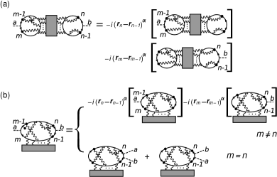
Figure 8: High-order interaction corrections to the spin current-current correlation function in class AIII. The equations shown are valid up to order of $\Omega$. (a) The current-current correlation function $\delta\Pi_{\alpha\alpha,mn}^{(\mathrm{a})}(i\Omega)$, where the two current density operators $j_{\alpha}(\mathbf{r}_{a})$ and $j_{\alpha}(\mathbf{r}_{b})$ locate on different fermion loops. (b) The current-current correlation function $\delta\Pi_{\alpha\alpha,mn}^{(\mathrm{b})}(i\Omega)$, where the current density operators are on one fermion loop.

Regardless of details, at a fixed perturbative order in interactions, a current-current correlation diagram should take the form of one of the two expressions as shown in Fig. 8. (a) The two current densities $j_{\alpha}(\mathbf{r}_{a})$ and $j_{\alpha}(\mathbf{r}_{b})$ are allocated on different fermion loops. For second order this corresponds to, for example, Fig. 7(d)(iii). (b) The two current densities are on the same fermion loop. For second order this corresponds to, for example, Fig. 7(c)(ii). Along a circular direction on the loops that support the current densities, we label the coordinates of interaction vertices as $\mathbf{r}_{1},\mathbf{r}_{2},\mathbf{r}_{3},...$, subsequently. Although we treat the $\{\mathbf{r}_{i}\}$ as independent labels, some of these are in fact constrained in pairs by the interaction. This does not affect the following argument.

As shown in Fig. 8(a), up to the order of $\Omega$, the correlation function $\delta\Pi_{\alpha\alpha,mn}^{(\mathrm{a})}(i\Omega)$ splits into two terms due to the Ward identity (54b). For second order this decomposition corresponds to, for example, Eq. (86). Summing over the coordinate indices $m$ and $n$, one readily has

$$\sum_{n,m}\delta\Pi_{\alpha\alpha,mn}^{(\mathrm{a})}(i\Omega)=\mathcal{O}(\Omega^{2}),$$ (92)

since

$$\sum_{n\in\mathrm{loop}}(\mathbf{r}_{n}-\mathbf{r}_{n-1})^{\alpha}=0.$$ (93)

Therefore, the dc conductivity corrections arising from the diagrams in Fig. 8(a) vanish for all temperatures ZNA2001 .

As shown in Fig. 8(b), up to order of $\Omega$, the correlation function $\delta\Pi_{\alpha\alpha,mn}^{(\mathrm{b})}(i\Omega)$ has to be analyzed in two cases,

$$\delta\Pi_{\alpha\alpha,mn}^{(\mathrm{b})}(i\Omega)=\begin{cases}\delta\Pi_{\alpha\alpha,mn}^{(\mathrm{b}1)}(i\Omega),\quad m\neq n,\vspace{0.3cm}\\ \delta\Pi_{\alpha\alpha,n}^{(\mathrm{b}2)}(i\Omega),\quad m=n,\end{cases}$$ (94)

where the expressions of $\delta\Pi_{\alpha\alpha,mn}^{(\mathrm{b}1)}(i\Omega)$ and $\delta\Pi_{\alpha\alpha,n}^{(\mathrm{b}2)}(i\Omega)$ are shown in the figure respectively. Summing over the indices $m$ and $n$ we obtain

$$\sum_{n,m}\delta\Pi_{\alpha\alpha,mn}^{(\mathrm{b})}(i\Omega)=\sum_{n\neq m}\delta\Pi_{\alpha\alpha,mn}^{(\mathrm{b}1)}(i\Omega)+\sum_{n}\delta\Pi_{\alpha\alpha,n}^{(\mathrm{b}2)}(i\Omega)$$

$$=\sum_{n}\left[\delta\Pi_{\alpha\alpha,n}^{(\mathrm{b}2)}(i\Omega)-\delta{\Pi}_{\alpha\alpha,nn}^{(\mathrm{b}1)}(i\Omega)\right]+\mathcal{O}(\Omega^{2}),$$ (95)

where we have used $\sum_{n,m}\delta\Pi_{\alpha\alpha,mn}^{(\mathrm{b}1)}(i\Omega)=0$ due to the circular property (93). Defining a dressed propagator matrix analogous to $\hat{\mathcal{P}}_{43}(i\omega_{p})$ in Eq. (72) and repeating the procedure for evaluating the diagrams in Fig. 7(c)(i) and 7(c)(ii), one can show that at zero temperature the conductivity corrections arising from $\delta\Pi_{\alpha\alpha,n}^{(\mathrm{b}2)}(i\Omega)$ and $\delta{\Pi}_{\alpha\alpha,nn}^{(\mathrm{b}1)}(i\Omega)$ are identical for any $n$. The branch cut of the dressed propagator is on the real axis for all finite orders. Therefore, the zero-temperature conductivity corrections $\delta\sigma_{\mathrm{s},mn}^{\alpha\alpha}(\mathrm{b})$ cancel each other,

$$\sum_{n,m}\delta\sigma_{\mathrm{s},mn}^{\alpha\alpha}(\mathrm{b})=\mathcal{O}(\Omega^{2}).$$ (96)

We point out possible caveats of our analysis above. The precondition for applying the Ward identity is that the diagrams as shown in the brackets in Fig. 8 should be finite. Short-ranged interactions satisfy this precondition as long as the spin- and mass-squared operators are irrelevant at low energies. However, for Coulomb interactions these diagrams should exhibit an infrared divergence at any order (marginal) and eventually lead to a minimal dc conductivity SUP-MinCond-1 ; SUP-MinCond-2 ; SUP-MinCond-3 . For the disorder-free and noninteracting case, the Ward identity must also be used with care, since it leads to an ultraviolate divergence mirlin2006 . Moreover, the Taylor expansion based on the Ward identity (54a) applies in the dc limit ($\Omega\to 0$ before $T\to 0$) but fails in the optical limit ($\Omega\to 0$ after $T\to 0$).

V Large winding number expansion

V.1 Symmetry structure: replicated path integral

We write an imaginary time fermion path integral for Eq. (3) to encode disorder-averaged Green’s functions,

$$S\equiv \,S_{h}+S_{\epsilon},$$ (97a)

$$S_{h}= \,\int\!\frac{d\omega_{n}\mathrm{d}^{2}\mathbf{r}}{2\pi}\,\left[\begin{aligned} &\,\bar{L}\left(-i\bar{\partial}+\bar{A}_{j}\hat{\mathfrak{t}}^{j}+\bar{\mathcal{A}}\right)L\\ &\,+\bar{R}\left(-i\partial+A_{j}\hat{\mathfrak{t}}^{j}+\mathcal{A}\right)R\end{aligned}\right],$$ (97b)

$$S_{\epsilon}= \,\int\!\frac{d\omega_{n}\mathrm{d}^{2}\mathbf{r}}{2\pi}\,\left[-i\omega_{n}\left(\bar{L}R+\bar{R}L\right)\right],$$ (97c)

where $L\rightarrow L_{v,a}(\omega_{n},\bm{\mathrm{r}})$ carries color $v\in\{1,2,\ldots,|\nu|\}$ and replica $a\in\{1,2,\ldots,n\}$ indices. (Replicas are introduced to facilitate disorder averaging SUP-ASbook .) These are related to the fermion field in Eq. (3) via

$$\begin{aligned} \eta_{v,a}(\omega_{n},\bm{\mathrm{r}})=&\,\begin{bmatrix}L_{v,a}(\omega_{n},\bm{\mathrm{r}})\\ R_{v,a}(\omega_{n},\bm{\mathrm{r}})\end{bmatrix},\\ \bar{\eta}_{v,a}(\omega_{n},\bm{\mathrm{r}})=&\,\begin{bmatrix}\bar{R}_{v,a}(\omega_{n},\bm{\mathrm{r}})&\bar{L}_{v,a}(\omega_{n},\bm{\mathrm{r}})\end{bmatrix}.\end{aligned}$$ (98)

In Eq. (97), we have introduced the chiral notations

$$\begin{gathered}\{\partial,\bar{\partial}\}\equiv\partial_{x}\mp i\partial_{y},\\ \{A_{j},\bar{A}_{j}\}\equiv A_{j,x}\mp iA_{j,y},\;\;\{\mathcal{A},\bar{\mathcal{A}}\}\equiv\mathcal{A}_{x}\mp i\mathcal{A}_{y}.\end{gathered}$$

The structure of the low-energy effective theory for the critically delocalized SRFL2008 ; Foster2012 ; FXCup ; CFup surface Majorana fermions follows largely from symmetry analysis. As in standard localization physics, this will be a nonlinear sigma model with a target manifold determined by the set of transformations that preserves the action, in every fixed realization of disorder SUP-ASbook ; wm2008 ; foster0608 ; dellanna2006 . The manifold is the quotient of the symmetry of $S_{h}$ (the “Hamiltonian piece”) relative to the symmetry of $S$ foster0608 .

We consider class AIII. Equation (97b) is invariant under independent left and right unitary transformations

$$L\mapsto\hat{U}_{L}L,\;\;\bar{L}\mapsto\bar{L}\hat{U}_{L}^{\dagger},\;\;R\mapsto\hat{U}_{R}R,\;\;\bar{R}\mapsto\bar{R}\hat{U}_{R}^{\dagger}.$$ (99)

Here $\hat{U}_{L,R}$ are $\text{U}(nN)$ transformations that act on the product of replica $\otimes$ Matsubara frequency labels. ($N$ is the number of Matsubara frequencies. Formally we must take $N\rightarrow\infty$ and $n\rightarrow 0$, such that $Nn\rightarrow 0$.) The “energy piece” of the action $S_{\epsilon}$ further restricts $\hat{U}_{R}=\hat{U}_{L}$. Thus the target manifold is foster0608

$$\frac{\text{U}(nN)\times\text{U}(nN)}{\text{U}(nN)}\simeq\text{U}(nN).$$ (100)

Equation (100) is almost sufficient to determine the form of the nonlinear sigma model. The exact solution SUP-NTW1994 ; MCW96 ; CKT1996 to the noninteracting, disorder-only problem in $2+0$ dimensions via non-Abelian bosonization shows that the standard sigma model action must be supplemented by a Wess-Zumino-Novikov-Witten (WZNW) term at level $K$, where $K=|\nu|$ for class AIII FXCup . The analysis for classes CI and DIII is similar, leading to

$$\begin{array}[]{lcc}\textrm{Class }&\textrm{Target manifold }G&\textrm{WZNW level }K\\ \hline\cr\textrm{CI}&\textrm{Sp}(2nN)&|\nu|/2\\ \textrm{AIII}&\textrm{U}(nN)&|\nu|\\ \textrm{DIII}&\textrm{O}(nN)&|\nu|\\ \hline\cr\end{array}$$ (105)

V.2 Wess-Zumino-Novikov-Witten Finkel’stein nonlinear $\bm{\sigma}$ model

The Finkel’stein nonlinear sigma model with a WZNW term (WZNW-FNLsM) incorporates three sectors:

$$S[\hat{Q}]=S_{0}[\hat{Q}]+S_{\mathrm{I}}[\hat{Q}]+\Gamma_{K}[\hat{Q}],$$ (106)

where $S_{0}[\hat{Q}]$ represents the standard dynamical sigma model on the target manifold $G$ defined in Eq. (105), $S_{\mathrm{I}}[\hat{Q}]$ encodes the four-fermion interactions shown in Eq. (6), and $\Gamma_{K}[\hat{Q}]$ is the WZNW term at level $K$.

The WZNW term takes the unique form SUP-ASbook

$$\begin{split}\Gamma_{K}[\hat{Q}]=&-i\,K\int\!\frac{\mathrm{d}^{3}\mathbf{r}}{12\pi l_{\phi}}\,\epsilon^{\alpha\beta\gamma}\,\\ &\;\;\,\times\!\text{Tr}\left[(\hat{Q}^{-1}\partial_{\alpha}\hat{Q})(\hat{Q}^{-1}\partial_{\beta}\hat{Q})(\hat{Q}^{-1}\partial_{\gamma}\hat{Q})\right]\!,\end{split}$$ (107)

where the spatial integral is over the 3D bulk of a superconductor that is surrounded by the surface we are considering, and $l_{\phi}$ is the Dynkin index of the corresponding symmetry group,

$$l_{\phi}=1\;\;(\text{classes CI, AIII}),\quad l_{\phi}=2\;\;(\text{class DIII}).$$ (108)

The nontopological action and matrix field $\hat{Q}(\mathbf{r})$ target space distinguish the three universality classes.
(i) Class CI. $S_{0}[\hat{Q}]$ and $S_{\mathrm{I}}[\hat{Q}]$ take the forms dellanna2006

$$S_{0}[\hat{Q}]= \frac{1}{2\lambda}\int_{\mathbf{r}}\text{Tr}\left[\nabla\hat{Q}^{\dagger}(\mathbf{r})\cdot\nabla\hat{Q}(\mathbf{r})\right]$$

$$-h\int_{\mathbf{r}}\text{Tr}\left(|\hat{\omega}|\otimes\hat{\Sigma}^{3}\left[i\hat{Q}(\mathbf{r})-i\hat{Q}^{\dagger}(\mathbf{r})\right]\right),$$ (109a)

$$S_{\mathrm{I}}[\hat{Q}]= \sum_{a}\!\int_{\mathbf{r},\tau}\left[\frac{\Gamma_{\mathrm{s}}}{2}\left(\text{Tr}_{\mu}\left\{\hat{\bm{\mu}}\left[\hat{Q}_{\tau\,\tau}^{a\,a}(\mathbf{r})-(\hat{Q}^{\dagger})_{\tau\,\tau}^{a\,a}(\mathbf{r})\right]\right\}\right)^{2}\right.$$

$$\left.+\frac{\Gamma_{\mathrm{c}}}{2}\left\{\text{Tr}_{\mu}\left[\hat{Q}_{\tau\,\tau}^{a\,a}(\mathbf{r})+(\hat{Q}^{\dagger})_{\tau\,\tau}^{a\,a}(\mathbf{r})\right]\right\}^{2}\right].$$ (109b)

In Eq. (109), we introduce two sets of Pauli matrices: $\hat{\bm{\mu}}=(\hat{\mu}^{1},\hat{\mu}^{2},\hat{\mu}^{3})$ act on physical spin space, while $(\hat{\Sigma}^{1},\hat{\Sigma}^{2},\hat{\Sigma}^{3})$ act on the sign of the Matsubara frequency; i.e., $\left\langle{\omega_{n}}\right|\hat{\Sigma}^{3}\left|{\omega_{m}}\right\rangle=\delta_{m,n}\operatorname{sgn}(\omega_{m})$. $\hat{Q}(\mathbf{r})$ denotes a square matrix taking indices in replica space with $a,b\in\{1,2,\cdots,n\}$, physical spin space with $\mu,\mu^{\prime}\in\{\uparrow,\downarrow\}$, and the imaginary time $\tau,\tau^{\prime}$ or modulus Matsubara frequencies $|\omega|$, $|\omega^{\prime}|$ and their sign $\Sigma$, $\Sigma^{\prime}$ spaces:

$$\hat{Q}(\mathbf{r})\to\begin{cases}Q^{\mu a,\mu^{\prime}b}_{\tau,\tau^{\prime}}(\mathbf{r}),&\mbox{Temporal basis},\\ Q^{\mu a,\mu^{\prime}b}_{\Sigma|\omega|,\Sigma^{\prime}|\omega^{\prime}|}(\mathbf{r}),&\mbox{Frequency basis}.\end{cases}$$ (110)

The matrix field $\hat{Q}(\mathbf{r})$ belongs to Sp($2nN$) group, which satisfies the unitary condition

$$\hat{Q}^{\dagger}(\mathbf{r})\hat{Q}(\mathbf{r})=\hat{1},$$ (111a)

and in the temporal basis the symplectic condition

$$\hat{\mu}^{2}\,\hat{Q}^{\mathsf{T}}(\mathbf{r})\,\hat{\mu}^{2}=\hat{Q}^{\dagger}(\mathbf{r}).$$ (111b)

In a perturbative expansion, the physical saddle point is set by the frequency term in Eq. (109a) and is given by dellanna2006 ; foster0608

$$\hat{Q}_{\text{sp}}(\mathbf{r})=-i\hat{\Sigma}^{3}.$$ (112)

(ii) Class AIII. $S_{0}[\hat{Q}]$ and $S_{\mathrm{I}}[\hat{Q}]$ take the forms foster0608

$$S_{0}[\hat{Q}]= \,\frac{1}{2\lambda}\int_{\mathbf{r}}\text{Tr}\left[\nabla\hat{Q}^{\dagger}(\mathbf{r})\cdot\nabla\hat{Q}(\mathbf{r})\right]$$

$$\,-\frac{\lambda_{\mathrm{A}}}{2\lambda^{2}}\int_{\mathbf{r}}\text{Tr}\left[\hat{Q}^{\dagger}(\mathbf{r})\nabla\hat{Q}(\mathbf{r})\right]\cdot\text{Tr}\left[\hat{Q}^{\dagger}(\mathbf{r})\nabla\hat{Q}(\mathbf{r})\right]$$

$$\,-h\int_{\mathbf{r}}\text{Tr}\left(|\hat{\omega}|\otimes\hat{\Sigma}^{3}\left[i\hat{Q}(\mathbf{r})-i\hat{Q}^{\dagger}(\mathbf{r})\right]\right),$$ (113a)

$$S_{\mathrm{I}}[\hat{Q}]= \,\sum_{a}\!\int_{\mathbf{r},\tau}\left\{\Gamma_{\mathrm{s}}\left[\hat{Q}_{\tau\,\tau}^{a\,a}(\mathbf{r})-(\hat{Q}^{\dagger})_{\tau\,\tau}^{a\,a}(\mathbf{r})\right]^{2}\right.$$

$$\,\left.+\Gamma_{\mathrm{c}}\left[\hat{Q}_{\tau\,\tau}^{a\,a}(\mathbf{r})+(\hat{Q}^{\dagger})_{\tau\,\tau}^{a\,a}(\mathbf{r})\right]^{2}\right\}.$$ (113b)

In Eq. (113), $\hat{Q}(\mathbf{r})$ takes indices in replica space, and imaginary time or Matsubara frequency space:

$$\hat{Q}(\mathbf{r})\to\begin{cases}Q^{a,b}_{\tau,\tau^{\prime}}(\mathbf{r}),&\mbox{Temporal basis},\\ Q^{a,b}_{\Sigma|\omega|,\Sigma^{\prime}|\omega^{\prime}|}(\mathbf{r}),&\mbox{Frequency basis}.\end{cases}$$ (114)

The matrix field $\hat{Q}(\mathbf{r})\in\text{U}(nN)$ satisfies only the unitary constraint (111a). The saddle point of the sigma model still takes the form of Eq. (112).

The “Gade ” term SUP-Gade9193 in the second line of Eq. (113a) is special to class AIII. It is proportional to the disorder variance $\lambda_{A}$ of the Abelian vector potential in Eq. (3), taken to be Gaussian white noise correlated:

$$\overline{\mathcal{A}_{\alpha}(\mathbf{r})\mathcal{A}_{\beta}(\mathbf{r}^{\prime})} =\lambda_{A}\delta_{\alpha\beta}\,\delta^{(2)}(\mathbf{r}-\mathbf{r}^{\prime}).$$ (115)

(iii) Class DIII. In this class the form of $S_{0}[\hat{Q}]$ is the same as that of Eq. (109a), where the matrix field $\hat{Q}(\mathbf{r})$ possesses the same indices as those for class AIII [see Eq. (114)]. Because physical spin is not a conserved quantity any longer, $S_{\mathrm{I}}[\hat{Q}]$ only incorporates the Cooper interaction channel:

$$S_{\mathrm{I}}[\hat{Q}]=\sum_{a}\!\int_{\mathbf{r},\tau}\Gamma_{\mathrm{c}}\left[\hat{Q}_{\tau\,\tau}^{a\,a}(\mathbf{r})+(\hat{Q}^{\dagger})_{\tau\,\tau}^{a\,a}(\mathbf{r})\right]^{2}.$$ (116)

In the temporal basis, the matrix field $\hat{Q}(\mathbf{r})\in\text{O}(nN)$ satisfies the orthogonal condition

$$\hat{Q}^{\ast}(\mathbf{r})=\hat{Q}(\mathbf{r}),\quad\hat{Q}^{\mathsf{T}}(\mathbf{r})\hat{Q}(\mathbf{r})=\hat{1},$$ (117)

and the saddle point is given by Eq. (112).

V.3 One-loop renormalization group analysis

In the limit of large topological winding numbers $K\gg 1$, the WZNW-FNLsMs are amenable to a perturbative RG analysis with $1/K$ as the small parameter. In this section, we perform a one-loop RG calculation via the background field method, as employed in Ref. foster0608 .

We shift the saddle point in Eq. (112) to the identity:

$$\hat{Q}(\mathbf{r})\to-i\hat{\Sigma}^{3}\,\hat{Q}(\mathbf{r}),\quad\hat{Q}^{\dagger}(\mathbf{r})\to\hat{Q}^{\dagger}(\mathbf{r})\,i\hat{\Sigma}^{3},\quad\hat{Q}_{\text{sp}}(\mathbf{r})\to\hat{1}.$$ (118)

With respect to the transformation (118), the action of the sigma model does not change except for the frequency and interaction sectors: The frequency sector transforms as

$$\int_{\mathbf{r}}\text{Tr}\left[|\hat{\omega}|\otimes\hat{\Sigma}^{3}\left(i\hat{Q}-i\hat{Q}^{\dagger}\right)\right]\to\int_{\mathbf{r}}\text{Tr}\left[|\hat{\omega}|\left(\hat{Q}^{\dagger}+\hat{Q}\right)\right].$$ (119)

In frequency space, the interaction sector transforms as

$$S_{\mathrm{I}}[\hat{Q}]\to -\sum_{a}\!\int\limits_{\begin{subarray}{c}\omega_{1},\omega_{2}\\ \omega_{3},\omega_{4}\end{subarray}}\int_{\mathbf{r}}\delta_{1+3,2+4}$$ (120)

$$\times\Big{\{}\frac{\Gamma_{\mathrm{s}}}{2}\,\begin{aligned} &\text{Tr}_{\mu}\left[\hat{\bm{\mu}}\left(s_{1}\,\hat{Q}_{1,2}^{a,a}+s_{2}\left.\hat{Q}^{\dagger}\right._{1,2}^{a,a}\right)\right]\\ &\cdot\text{Tr}_{\mu}\left[\hat{\bm{\mu}}\left(s_{3}\,\hat{Q}_{3,4}^{a,a}+s_{4}\left.\hat{Q}^{\dagger}\right._{3,4}^{a,a}\right)\right]\end{aligned}$$

$$\phantom{\Big{\{}}+\frac{\Gamma_{\mathrm{c}}}{2}\,\begin{aligned} &\text{Tr}_{\mu}\left[\left(s_{1}\,\hat{Q}_{1,2}^{a,a}-s_{2}\left.\hat{Q}^{\dagger}\right._{1,2}^{a,a}\right)\right]\\ &\times\text{Tr}_{\mu}\left[\left(s_{3}\,\hat{Q}_{3,4}^{a,a}-s_{4}\left.\hat{Q}^{\dagger}\right._{3,4}^{a,a}\right)\right]\Big{\}},\end{aligned}\!\!$$

in class CI, and similarly in classes AIII and DIII. The abbreviated symbols in Eq. (120) are defined as

$$\begin{aligned} &\hat{Q}_{1,2}^{a,b}\equiv\hat{Q}_{\omega_{1},\omega_{2}}^{a,b},\\ &\delta_{1+3,2+4}\equiv 2\pi\delta(\omega_{1}+\omega_{3}-\omega_{2}-\omega_{4}),\\ &\int\limits_{\omega_{1},\omega_{2},\ldots}\equiv\int\frac{d\omega_{1}}{2\pi}\int\frac{d\omega_{2}}{2\pi}\times\cdots,\\ &s_{\alpha}\equiv\text{sgn}(\omega_{\alpha}),\quad\alpha\in\{1,2,3,4\}.\end{aligned}$$ (121)

We split $\hat{Q}$ into “fast” $\hat{Q}_{\mathsf{F}}$ and “slow” $\hat{Q}_{\mathsf{S}}$ modes,

$$\hat{Q}(\mathbf{r})=\hat{Q}_{\mathsf{F}}(\mathbf{r})\,\hat{Q}_{\mathsf{S}}(\mathbf{r})=\hat{Q}_{\mathsf{F}}(\mathbf{r})\left[\hat{1}+\delta{\hat{Q}_{\mathsf{S}}(\mathbf{r})}\right],$$ (122)

where $\hat{Q}_{\mathsf{F},\mathsf{S}}(\mathbf{r})$ belong to the same symmetry group as $\hat{Q}(\mathbf{r})$. We further decompose the slow field into the homogeneous saddle point “$\hat{1}$” plus a slow variation $\delta\hat{Q}_{\mathsf{S}}(\mathbf{r})$. The fast field $\hat{Q}_{\mathsf{F}}(\mathbf{r})$ will be parameterized by unconstrained coordinates $\hat{Y}(\mathbf{r})$. The slow mode fluctuation $\delta\hat{Q}_{\mathsf{S}}({\bf k})\to\delta\hat{Q}_{\mathsf{S}\omega,\omega^{\prime}}^{a,a^{\prime}}({\bf k})$ possesses support within a cube of linear size $\tilde{\Lambda}$ in the space $\left(|\omega|,\,|\omega^{\prime}|,\,D{\bf k}^{2}\right)$ foster0608 , where

$$D=1/(\lambda h)$$ (123)

is the heat diffusion constant. The fast mode coordinates $\hat{Y}({\bf k})\to\hat{Y}_{\omega,\omega^{\prime}}^{a,a^{\prime}}({\bf k})$ lie within a surrounding shell of thickness $\Lambda-\tilde{\Lambda}$. Here $\Lambda/\tilde{\Lambda}\approx 1+2\mathrm{d}\ell$ is a ratio of energy cutoffs with $0<\mathrm{d}\ell\ll 1$.

Via Eq. (122) the action is

$$S[\hat{Q}]=S_{\mathsf{S}}[\hat{Q}_{\mathsf{S}}]+S_{\mathsf{F}}[\hat{Q}_{\mathsf{F}}]+S_{\mathsf{S}/\mathsf{F}}[\delta\hat{Q}_{\mathsf{S}},\hat{Q}_{\mathsf{F}}],$$ (124)

where

$$S_{\mathsf{S}}[\hat{Q}_{\mathsf{S}}]=S[\hat{Q}\to\hat{Q}_{\mathsf{S}}].$$ (125)

The topological number $K$ enters into the renormalization equations only for the disorder parameters $\lambda$ and $\lambda_{\mathrm{A}}$ (the latter only for class AIII), because the WZNW term modifies only the “stiffness” vertex. The interaction parameters $\Gamma_{\mathrm{s}}$ (classes CI and AIII) and $\Gamma_{\mathrm{c}}$ obey the same RG equations as those for the FNLsM lacking the WZNW term in the corresponding symmetry class foster0608 ; dellanna2006 . In the remainder, we only present the components of $S_{\mathsf{S}/\mathsf{F}}[\delta\hat{Q}_{\mathsf{S}},\hat{Q}_{\mathsf{F}}]$ that renormalize the disorder parameters $\lambda$ and $\lambda_{\mathrm{A}}$.

V.3.1 Spin U(1) symmetry: Class AIII

(i) Parametrization and Feynman rules. We parametrize the fast field $\hat{Q}_{\mathsf{F}}(\mathbf{r})$ by

$$\begin{split}\hat{Q}_{\mathsf{F}}(\mathbf{r})=&\,\exp{[i\hat{Y}(\mathbf{r})]}\\ =&\,\hat{1}+i\,\hat{Y}(\mathbf{r})-\frac{1}{2}\hat{Y}^{2}(\mathbf{r})+\mathcal{O}[\|\hat{Y}\|^{3}],\end{split}$$ (126)

where $\hat{Y}$ is a Hermitian matrix belonging to the unitary Lie algebra $\mathfrak{u}(nN)$:

$$\hat{Y}^{\dagger}=\hat{Y}.$$ (127)

Substituting Eq. (122) together with Eq. (126) into the action described by Eqs. (106), (107), and (113), and retaining up to quadratic terms in the fast mode coordinates $\hat{Y}(\mathbf{r})$, we obtain the fast mode action:

$$S_{\mathsf{F}}[\hat{Y}]=S_{\mathsf{F}}^{(0)}[\hat{Y}]+S_{\mathsf{F}}^{(\mathrm{I})}[\hat{Y}],$$ (128)

where

$$S_{\mathsf{F}}^{(0)}[\hat{Y}]=\, \frac{1}{2}\int_{\mathbf{r}}\text{Tr}\left[\frac{1}{\lambda}(\nabla\hat{Y})^{2}+h\,|\hat{\omega}|\,\hat{Y}^{2}+h\,\hat{Y}\,|\hat{\omega}|\,\hat{Y}\right]$$

$$+\frac{\lambda_{A}}{2\lambda^{2}}\int_{\mathbf{r}}\text{Tr}(\nabla\hat{Y})\cdot\text{Tr}(\nabla\hat{Y}),$$ (129a)

$$S_{\mathsf{F}}^{(\mathrm{I})}[\hat{Y}]=\, \sum_{a}\int\limits_{\begin{subarray}{c}\omega_{1},\omega_{2}\\ \omega_{3},\omega_{4}\end{subarray}}\int_{\mathbf{r}}\delta_{1+3,2+4}\left[\Gamma_{\mathrm{s}}\,(s_{1}-s_{2})\,(s_{3}-s_{4})\right.$$

$$\left.+\Gamma_{\mathrm{c}}\,(s_{1}+s_{2})\,(s_{3}+s_{4})\right]\,Y_{1,2}^{a,a}\,Y_{3,4}^{a,a}.$$ (129b)

with $S_{\mathsf{F}}^{(0)}$ and $S_{\mathsf{F}}^{(\mathrm{I})}$ arising from Eqs. (113a) and (113b), respectively.

The fast field propagator decomposes into foster0608 ,

$$\Big{\langle}Y_{1,2}^{a,b} (-\mathbf{k})\,Y_{3,4}^{c,d}(\mathbf{k})\Big{\rangle}=\mathsf{P}_{\lambda}+\mathsf{P}_{\mathrm{A}}+\mathsf{P}_{\mathrm{s}}+\mathsf{P}_{\mathrm{c}},$$ (130a)

$$\mathsf{P}_{\lambda}= \,\Delta_{\mathrm{O}}(|\omega_{1}|,|\omega_{2}|,\mathbf{k})\delta_{1,4}\delta_{2,3}\delta_{ad}\delta_{bc},$$ (130b)

$$\mathsf{P}_{\mathrm{A}}= \,-\frac{\lambda_{\mathrm{A}}}{\lambda^{2}}\mathbf{k}^{2}\Delta_{\mathrm{O}}(|\omega_{1}|,|\omega_{1}|,\mathbf{k})\,\Delta_{\mathrm{O}}(|\omega_{3}|,|\omega_{3}|,\mathbf{k})$$

$$\,\phantom{-}\times\delta_{1,2}\delta_{3,4}\delta_{ab}\delta_{cd},$$ (130c)

$$\mathsf{P}_{\mathrm{s}}= \,-2\,\Gamma_{\mathrm{s}}(s_{1}-s_{2})(s_{3}-s_{4})\delta_{1+3,2+4}\delta_{ab}\delta_{bc}\delta_{cd}$$

$$\,\phantom{-}\times\Delta_{\mathrm{O}}(|\omega_{1}-\omega_{2}|,0,\mathbf{k})\,\Delta_{\mathrm{S}}(|\omega_{1}-\omega_{2}|,\mathbf{k}),$$ (130d)

$$\mathsf{P}_{\mathrm{c}}= \,-2\,\Gamma_{\mathrm{c}}(s_{1}+s_{2})(s_{3}+s_{4})\delta_{1+3,2+4}\delta_{ab}\delta_{bc}\delta_{cd}$$

$$\,\phantom{-}\times\frac{\Delta_{\mathrm{O}}(|\omega_{1}|,|\omega_{2}|,\mathbf{k})\,\Delta_{\mathrm{O}}(|\omega_{3}|,|\omega_{4}|,\mathbf{k})}{1+\gamma_{\mathrm{c}}f(|\omega_{1}-\omega_{2}|,{\bf k},\Lambda)},$$ (130e)

where

$$\Delta_{\mathrm{O}}(|\omega_{1}|,|\omega_{2}|,\mathbf{k})= \,\frac{1}{h}\frac{1}{D\mathbf{k}^{2}+(|\omega_{1}|+|\omega_{2}|)},$$ (131a)

$$\Delta_{\mathrm{S}}(|\omega|,\mathbf{k})= \,\frac{1}{h}\frac{1}{D\mathbf{k}^{2}+(1-\gamma_{\mathrm{s}})|\omega|}.$$ (131b)

In Eqs. (131b) and (130e) and the following, $\gamma_{\mathrm{s},\mathrm{c}}$ are defined by

$$\gamma_{\mathrm{s},\mathrm{c}}\equiv\frac{4\Gamma_{\mathrm{s},\mathrm{c}}}{\pi h}.$$ (132)

The function $f(|\omega|,{\bf k},\Lambda)$ appearing in $\mathsf{P}_{\mathrm{c}}$ reads

$$f(|\omega|,{\bf k},\Lambda)=\ln\left(\frac{2\Lambda}{D{\bf k}^{2}+|\omega|}\right),$$ (133)

with $\Lambda$ being the hard cutoff in frequency-momentum space foster0608 . We note that in Eq. (130e) and in the following, the Cooper channel propagator $\mathsf{P}_{\mathrm{c}}$ (and $\tilde{\mathsf{P}}_{\mathrm{c}}$ for class CI) is evaluated up to logarithmic accuracy in the cutoff $\Lambda$. The propagators are depicted in Fig. 9.

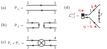
Figure 9: Feynman rules for class AIII. (a)–(c) Fast field propagators taking the corresponding expressions in Eq. (130). (d) Stiffness vertex arising from the coupling between fast and slow fields represented by Eq. (134). The numeric labels appearing at the terminals of fermion lines encode replica and frequency indices of fast field $\hat{Y}$. For the vertex in panel (d) the index “$3^{\prime}$” can carry a fast frequency, while “$1$” and “$2$” carry only the slow ones.

The fast and slow modes are coupled by the term $S_{\mathsf{S}/\mathsf{F}}[\delta\hat{Q}_{\mathsf{S}},\hat{Q}_{\mathsf{F}}]$ in Eq. (124). Equations (107) and (113a) give the stiffness vertex shown in Fig. 9(d),

$$\begin{split}S_{\mathsf{S}/\mathsf{F}}^{(0)}=&\frac{1}{2\lambda}\int_{\mathbf{r}}\left(\delta^{\alpha\beta}+\frac{i\lambda K}{4\pi l_{\phi}}{\epsilon}^{\alpha\beta}\right)\text{Tr}\left\{\hat{Q}_{\mathsf{S}}\left(\partial_{\alpha}\hat{Q}_{\mathsf{S}}^{\dagger}\right)\left[\hat{Y},\partial_{\beta}\hat{Y}\right]\right\}\\ =&\int\frac{d^{2}\mathbf{k}}{(2\pi)^{2}}\int\frac{d^{2}\mathbf{q}}{(2\pi)^{2}}\text{Tr}\left[\hat{Y}(-\mathbf{k}-\mathbf{q})\,\hat{\mathcal{L}}(\mathbf{k},\mathbf{q})\,\hat{Y}(\mathbf{k})\right],\end{split}$$ (134a)

where

$$\hat{\mathcal{L}}(\mathbf{k},\mathbf{q})=\frac{i}{2\lambda}\left[(2\mathbf{k}+\mathbf{q})-\frac{i\lambda K}{4\pi l_{\phi}}(2\mathbf{k}+\mathbf{q})\times\mathbf{e}_{z}\right]\cdot\hat{\mathbf{L}}(\mathbf{q}),$$ (134b)

with $$\hat{Y}(\mathbf{k}) \hat{\mathbf{L}}(\mathbf{q}) \hat{Y}(\mathbf{r})$$ and being the Fourier transforms of the fast field and the vector operator

$$\hat{\mathbf{L}}(\mathbf{r})=\hat{Q}_{\mathsf{S}}(\mathbf{r})\nabla\hat{Q}_{\mathsf{S}}^{\dagger}(\mathbf{r}),$$ (134c)

respectively. The stiffness vertex in classes DIII or CI takes a similar form as in Eq. (134). We only need this vertex to derive the one-loop renormalization equations for the spin resistance $\lambda$ and the Gade parameter $\lambda_{\mathrm{A}}$. A full list of vertices coupling fast and slow modes (in the Keldysh formalism) can be found in Ref. foster0608 .

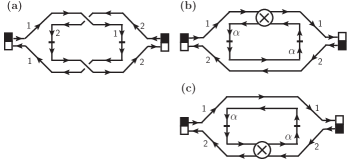
Figure 10: Category $\mathfrak{D}_{\text{AIII}}$: Diagrams renormalizing $\lambda$ and $\lambda_{\mathrm{A}}$ for class AIII in the replica limit $n\to 0$. $\mathfrak{D}_{\text{AIII}}$(a) renormalizes $\lambda_{\mathrm{A}}$, and $\mathfrak{D}_{\text{AIII}}$(b) and $\mathfrak{D}_{\text{AIII}}$(c) renormalize $\lambda$.

(ii) Renormalization of $\lambda$ and $\lambda_{\mathrm{A}}$. Diagram $\mathfrak{D}_{\text{AIII}}$(a) appearing in Fig. 10 renormalizes $\lambda_{\mathrm{A}}$,

$$\mathfrak{D}_{\text{AIII}}(\text{a})=F\int_{\mathbf{r}}[\text{Tr}(\hat{Q}_{\mathsf{S}}\nabla\hat{Q}_{\mathsf{S}}^{\dagger})]^{2},$$ (135)

where

$$F\equiv\left(\frac{\mathrm{d}\ell}{8\pi}\right)\bigg{[}1-\left(\frac{\lambda K}{4\pi l_{\phi}}\right)^{2}\bigg{]}.$$ (136)

Diagrams $\mathfrak{D}_{\text{AIII}}$(b) and $\mathfrak{D}_{\text{AIII}}$(c) in Fig. 10 renormalize the spin resistance $\lambda$,

$$\begin{split}&\mathfrak{D}_{\text{AIII}}\text{(b)}+\mathfrak{D}_{\text{AIII}}\text{(c)}\\ &=F\left\{2\left[1+\frac{1-\gamma_{\mathrm{s}}}{\gamma_{\mathrm{s}}}\ln(1-\gamma_{\mathrm{s}})\right]-\frac{1}{2}\mathcal{K}(\gamma_{\mathrm{c}})\right\}\\ &\quad\times\int_{\mathbf{r}}\text{Tr}(\nabla\hat{Q}_{\mathsf{S}}^{\dagger}\cdot\nabla\hat{Q}_{\mathsf{S}}),\end{split}$$ (137)

where

$$\mathcal{K}(\gamma_{\mathrm{c}})=2e^{-1/\gamma_{\mathrm{c}}}\left[E_{i}\left(\frac{1}{\gamma_{\mathrm{c}}}+\ln 2\right)-E_{i}\left(\frac{1}{\gamma_{\mathrm{c}}}\right)\right]$$ (138)

with $E_{i}(z)$ being the exponential integral.

(iii) Full one-loop RG equations. Substituting $l_{\phi}=1$ [Eq. (108)] into Eqs. (135) and (137) and performing a trivial rescaling,

$$\lambda\to 4\pi\lambda,\quad\lambda_{\mathrm{A}}\to 4\pi\lambda_{\mathrm{A}},$$ (139)

we obtain the one-loop RG equations for class AIII:

$$\frac{\mathrm{d}\lambda}{\mathrm{d}\ell}= \,\lambda^{2}\left[1-(K\lambda)^{2}\right]\mathcal{I}(\gamma_{\mathrm{s}},\gamma_{\mathrm{c}}),$$ (140a)

$$\frac{\mathrm{d}\lambda_{\mathrm{A}}}{\mathrm{d}\ell}= \,\lambda^{2}\left[1-(K\lambda)^{2}\right]\left[1+\frac{2\lambda_{\mathrm{A}}}{\lambda}\mathcal{I}(\gamma_{\mathrm{s}},\gamma_{\mathrm{c}})\right],$$ (140b)

$$\frac{\mathrm{d}\gamma_{\mathrm{s}}}{\mathrm{d}\ell}= \,(1-\gamma_{\mathrm{s}})\left[\lambda_{\mathrm{A}}(\gamma_{\mathrm{s}}+2\gamma_{\mathrm{c}}-2\gamma_{\mathrm{s}}\gamma_{\mathrm{c}})\right.$$

$$\left.-\lambda(\gamma_{\mathrm{s}}+\gamma_{\mathrm{c}}-2\gamma_{\mathrm{s}}\gamma_{\mathrm{c}})\right],$$ (140c)

$$\frac{\mathrm{d}\gamma_{\mathrm{c}}}{\mathrm{d}\ell}= \,\lambda_{\mathrm{A}}(2\gamma_{\mathrm{s}}+\gamma_{\mathrm{c}})-\lambda(\gamma_{\mathrm{s}}+\gamma_{\mathrm{c}})$$

$$+\lambda\left[2\gamma_{\mathrm{c}}\ln{(1-\gamma_{\mathrm{s}})}+\gamma_{\mathrm{s}}\gamma_{\mathrm{c}}\right]-2\gamma_{\mathrm{c}}^{2},$$ (140d)

where

$$\mathcal{I}(\gamma_{\mathrm{s}},\gamma_{\mathrm{c}})=2\left[1+\left(\frac{1-\gamma_{\mathrm{s}}}{\gamma_{\mathrm{s}}}\right)\ln{(1-\gamma_{\mathrm{s}})}\right]-\frac{1}{2}\mathcal{K}(\gamma_{\mathrm{c}}),$$ (141)

is the interaction correction to the dc conductivity. The RG equations for $\gamma_{\mathrm{s}}$ and $\gamma_{\mathrm{c}}$ in Eqs. (140c) and (140d) have been obtained in Ref. foster0608 and are computed only to the lowest nontrivial order in $\lambda$ and $\gamma_{\mathrm{c}}$. The implications of Eq. (140) for the stability of class AIII surface states were discussed in Ref. FXCup .

V.3.2 No spin symmetry: Class DIII

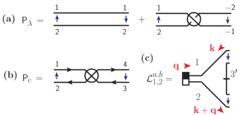
Figure 11: Feynman rules for class DIII. (a) The propagator $\mathsf{P}_{\lambda}$ in Eq. (146b). The first (second) diagram is associated with the contraction rule $\delta_{1,4}\delta_{2,3}\delta_{ad}\delta_{bc}$ ($\delta_{1,-3}\delta_{2,-4}\delta_{ac}\delta_{bd}$). We use the “blob” to indicate sign flips of frequencies. (b) The propagator $\mathsf{P}_{\mathrm{c}}$ in Eq. (146c). The diagram represents the term with the frequency conservation law $\delta_{1+3,2+4}$. (c) The stiffness vertex represented by Eq. (134) supplemented with a minus sign.

(i) Parametrization and Feynman rules. For class DIII the fast field $\hat{Q}_{\mathsf{F}}\in\text{O}(nN)$ can be parametrized by the so-called “$\sigma$-$\pi$” coordinates:

$$\begin{split}\hat{Q}_{\mathsf{F}}(\mathbf{r})=&\,\hat{Y}(\mathbf{r})+[\hat{1}+\hat{Y}^{2}(\mathbf{r})]^{1/2}\\ =&\,\hat{1}+\hat{Y}(\mathbf{r})+\frac{1}{2}\hat{Y}^{2}(\mathbf{r})+\mathcal{O}(\|\hat{Y}\|^{3}),\end{split}$$ (142)

where $\hat{Y}$ satisfies the antisymmetric condition in the frequency basis [Eq. (114)]

$$\hat{Y}^{\mathsf{T}}=-\hat{\Sigma}^{1}\hat{Y}\hat{\Sigma}^{1}.$$ (143)

The fast mode action is

$$S_{\mathsf{F}}[\hat{Y}]=S_{\mathsf{F}}^{(0)}[\hat{Y}]+S_{\mathsf{F}}^{(\mathrm{I})}[\hat{Y}],$$ (144)

where

$$S_{\mathsf{F}}^{(0)}[\hat{Y}]=\, -\frac{1}{2}\int_{\mathbf{r}}\text{Tr}\left[\frac{1}{\lambda}(\nabla\hat{Y})^{2}+h\,|\hat{\omega}|\,\hat{Y}^{2}+h\,\hat{Y}\,|\hat{\omega}|\,\hat{Y}\right],$$ (145a)

$$S_{\mathsf{F}}^{(\mathrm{I})}[\hat{Y}]=\, -\sum_{a}\int\limits_{\begin{subarray}{c}\omega_{1},\omega_{2}\\ \omega_{3},\omega_{4}\end{subarray}}\int_{\mathbf{r}}\delta_{1+3,2+4}$$

$$\times\Gamma_{\mathrm{c}}\,(s_{1}+s_{2})\,(s_{3}+s_{4})\,Y_{1,2}^{a,a}\,Y_{3,4}^{a,a},$$ (145b)

with $S_{\mathsf{F}}^{(0)}$ and $S_{\mathsf{F}}^{(\mathrm{I})}$ arising from Eqs. (109a) and (116), respectively. We note that Eq. (145b) only incorporates the Cooper interaction channel. The propagators are

$$\Big{\langle}Y_{1,2}^{a,b} (-\mathbf{k})\,Y_{3,4}^{c,d}(\mathbf{k})\Big{\rangle}=\mathsf{P}_{\lambda}+\mathsf{P}_{\mathrm{c}},$$ (146a)

$$\mathsf{P}_{\lambda}= \,-\frac{1}{2}\left(1-\delta_{1,-2}\delta_{ab}\right)$$

$$\phantom{-}\times\left(\delta_{1,4}\delta_{2,3}\delta_{ad}\delta_{bc}-\delta_{1,-3}\delta_{2,-4}\delta_{ac}\delta_{bd}\right)$$

$$\phantom{-}\times\Delta_{\mathrm{O}}(|\omega_{1}|,|\omega_{2}|,\mathbf{k}),$$ (146b)

$$\mathsf{P}_{\mathrm{c}}= \,2\Gamma_{\mathrm{c}}\,(s_{1}+s_{2})(s_{3}+s_{4})\delta_{1+3,2+4}\delta_{ab}\delta_{bc}\delta_{cd}$$

$$\,\times\frac{\Delta_{\mathrm{O}}(|\omega_{1}|,|\omega_{2}|,\mathbf{k})\,\Delta_{\mathrm{O}}(|\omega_{3}|,|\omega_{4}|,\mathbf{k})}{1+\gamma_{\mathrm{c}}f(|\omega_{1}-\omega_{2}|,{\bf k},\Lambda)},$$ (146c)

where $\Delta_{\mathrm{O}}(|\omega_{1}|,|\omega_{2}|,\mathbf{k})$ and $f(|\omega|,{\bf k},\Lambda)$ are defined in Eqs. (131a) and (133), respectively. Note that $\mathsf{P}_{\lambda}$ and $\mathsf{P}_{\mathrm{c}}$ are antisymmetric [Eq. (143)] in frequency and replica spaces and hence possess vanishing diagonal terms. The spin diffusion kernel $\Delta_{\mathrm{S}}(|\omega|,\mathbf{k})$ [Eq. (131b)] is absent compared to class AIII since spin is not conserved in DIII.

In Fig. 11(a) we represent the two components of $\mathsf{P}_{\lambda}$ as the two diagrams that exhibit the corresponding frequency and replica structures: the first diagram corresponds to $\delta_{1,4}\delta_{2,3}\delta_{ad}\delta_{bc}$ and the second to $\delta_{1,-3}\delta_{2,-4}\delta_{ac}\delta_{bd}$ [Eq. (146b)]. Notice that the first diagram should carry a minus sign. The propagator $\mathsf{P}_{\mathrm{c}}$ is represented by the diagram in Fig. 11(b). The arrows along the fermion lines indicate the frequency combination $\delta_{1+3,2+4}$ [Eq. (146c)]. The stiffness vertex, as pictured in Fig. 11(c), takes the form of Eq. (134b) with a sign flip $\hat{\mathcal{L}}(\mathbf{k},\mathbf{q})\to-\hat{\mathcal{L}}(\mathbf{k},\mathbf{q})$ and satisfies the antisymmetric constraint $\hat{\mathcal{L}}^{\mathsf{T}}=-\hat{\Sigma}^{1}\hat{\mathcal{L}}\hat{\Sigma}^{1}$ in frequency and replica space.

(ii) Renormalization of $\lambda$. The one-loop diagrams that renormalize $\lambda$ are depicted in Fig. 12. $\mathfrak{D}_{\text{DIII}}$(a) and $\mathfrak{D}_{\text{DIII}}$(b) involve only $\mathsf{P}_{\lambda}$ and give identical contributions. At finite replica ($n\neq 0$) we obtain

$$\begin{split}\mathfrak{D}_{\text{DIII}}&\text{(a)}+\mathfrak{D}_{\text{DIII}}\text{(b)}\\ =&\frac{F(nN-2)}{2}\int_{\mathbf{r}}\text{Tr}(\nabla\hat{Q}_{\mathsf{S}}^{\dagger}\cdot\nabla\hat{Q}_{\mathsf{S}}),\end{split}$$ (147)

where $N$ is the number of Matsubara frequencies, and $F$ is defined by Eq. (136). In Eq. (147) the prefactor “$nN-2$” arises from the replica-frequency loop, where the diagonal terms of the two propagators are removed due to the factor “$1-\delta_{1,-2}\delta_{ab}$” in Eq. (146b) SUP-rep-d3 .

Diagrams $\mathfrak{D}_{\text{DIII}}$(c)–$\mathfrak{D}_{\text{DIII}}$(f) in Fig. 12 incorporate one basic diffusion operator $\mathsf{P}_{\lambda}$ and one interaction-dressed operator $\mathsf{P}_{\mathrm{c}}$, and give identical contributions:

$$\begin{split}\sum_{\mathfrak{d}=\text{c}}^{\text{f}}\mathfrak{D}_{\text{DIII}}(\mathfrak{d})=&-\frac{F}{2}\mathcal{K}\left(\gamma_{\mathrm{c}}\right)\int_{\mathbf{r}}\text{Tr}(\nabla\hat{Q}_{S}^{\dagger}\cdot\nabla\hat{Q}_{S}),\end{split}$$ (148)

which can be understood as the Altshuler-Aronov correction by Cooper interactions. The function $\mathcal{K}\left(\gamma\right)$ is defined in Eq. (138).

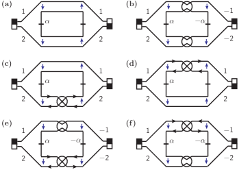
Figure 12: Category $\mathfrak{D}_{\text{DIII}}$: Diagrams renormalizing $\lambda$ in class DIII. (a) and (b) Weak antilocalization contribution [Eq. (147)]. (c)–(f) Altshuler-Aronov correction [Eq. (148)].

(iii) One-loop RG equation for $\lambda$. Substituting $l_{\phi}=2$ [Eq. (108)] into Eqs. (147) and (148), taking the replica limit $n\to 0$, and performing a trivial rescaling

$$\lambda\to 8\pi\lambda,$$ (149)

we obtain the RG equation for $\lambda$:

$$\frac{\mathrm{d}\lambda}{\mathrm{d}\ell}=\,-\lambda^{2}\left[1-(K\lambda)^{2}\right]\left[2+\mathcal{K}\left(\gamma_{\mathrm{c}}\right)\right].$$ (150)

In class DIII the Cooper interactions are always irrelevant FXCup , so we do not compute the full beta function for $\gamma_{\mathrm{c}}$.

V.3.3 Spin SU(2) symmetry: Class CI

(i) Parametrization and Feynman rules. We parametrize the fast field $\hat{Q}_{\mathsf{F}}\in\text{Sp}(2nN)$ via Eq. (126). In the frequency basis, the unitary and symplectic conditions (111a) and (111b) imply

$$\hat{Y}^{\dagger}=\hat{Y},\quad\hat{Y}^{\mathsf{T}}=-(\hat{\mu}^{2}\otimes\hat{\Sigma}^{1})\,\hat{Y}\,(\hat{\mu}^{2}\otimes\hat{\Sigma}^{1}).$$ (151)

As a consequence, $\hat{Y}$ takes the following block form in spin space:

$$\hat{Y}=\frac{1}{\sqrt{2}}\left(i\hat{W}_{0}\otimes\hat{1}+\sum_{\alpha=1}^{3}\hat{W}_{\alpha}\otimes\hat{\mu}^{\alpha}\right),$$ (152)

where the $nN\times nN$ matrices $\hat{W}_{\mathrm{j}=0,1,2,3}$ satisfy

$$\begin{split}\hat{W}_{0}^{\dagger}=-\hat{W}_{0},&\,\quad\hat{W}_{0}^{\mathsf{T}}=-\hat{\Sigma}^{1}\,\hat{W}_{0}\,\hat{\Sigma}^{1},\\ \hat{W}_{\alpha}^{\dagger}=\hat{W}_{\alpha},&\,\quad\hat{W}_{\alpha}^{\mathsf{T}}=\hat{\Sigma}^{1}\,\hat{W}_{\alpha}\,\hat{\Sigma}^{1},\end{split}$$ (153)

with $\alpha\in\{1,2,3\}$. The parametrization (152) naturally separates the interactions to one Cooper channel and three equivalent spin channels as shown in Eqs. (155b) and (155d).

The fast mode action consists of four decoupled modes described by the matrix fields $\hat{W}_{\mathrm{j}=0,1,2,3}$:

$$S_{\mathsf{F}}[\{\hat{W}_{\mathrm{j}}\}]=\sum_{\mathrm{j}=0}^{3}\left(S_{\mathsf{F},\mathrm{j}}^{(0)}[\hat{W}_{\mathrm{j}}]+S_{\mathsf{F},\mathrm{j}}^{(\text{I})}[\hat{W}_{\mathrm{j}}]\right),$$ (154)

where the antisymmetric sector $\hat{W}_{0}$ reads

$$S_{\mathsf{F},0}^{(0)}[\hat{W}_{0}]= \,-\frac{1}{2}\int_{\mathbf{r}}\widetilde{\text{Tr}}\left[\frac{1}{\lambda}(\nabla\hat{W}_{0})^{2}+h\,|\hat{\omega}|\,\hat{W}_{0}^{2}\right.$$

$$\left.+h\,\hat{W}_{0}\,|\hat{\omega}|\,\hat{W}_{0}\right],$$ (155a)

$$S_{\mathsf{F},0}^{(\text{I})}[\hat{W}_{0}]= \,-\,\sum_{a}\int\limits_{\begin{subarray}{c}\omega_{1},\omega_{2}\\ \omega_{3},\omega_{4}\end{subarray}}\int_{\mathbf{r}}\delta_{1+3,2+4}$$

$$\times\Gamma_{\mathrm{c}}(s_{1}+s_{2})\,(s_{3}+s_{4})\,[W_{0}]_{1,2}^{a,a}\,[W_{0}]_{3,4}^{a,a},$$ (155b)

and the symmetric sectors $$\hat{W}_{\alpha=1,2,3}$$ read

$$S_{\mathsf{F},\alpha}^{(0)}[\hat{W}_{\alpha}]= \,\frac{1}{2}\int_{\mathbf{r}}\widetilde{\text{Tr}}\left[\frac{1}{\lambda}(\nabla\hat{W}_{\alpha})^{2}+h\,|\hat{\omega}|\,\hat{W}_{\alpha}^{2}\right.$$

$$\left.+h\,\hat{W}_{\alpha}\,|\hat{\omega}|\,\hat{W}_{\alpha}\right],$$ (155c)

$$S_{\mathsf{F},\alpha}^{(\text{I})}[\hat{W}_{\alpha}]= \,\,\,\sum_{a}\int\limits_{\begin{subarray}{c}\omega_{1},\omega_{2}\\ \omega_{3},\omega_{4}\end{subarray}}\int_{\mathbf{r}}\delta_{1+3,2+4}$$

$$\times\Gamma_{\mathrm{s}}(s_{1}-s_{2})\,(s_{3}-s_{4})\,[W_{\alpha}]_{1,2}^{a,a}\,[W_{\alpha}]_{3,4}^{a,a}.$$ (155d)

In Eq. (155), $S_{\mathsf{F},\mathrm{j}}^{(0)}$ and $S_{\mathsf{F},\mathrm{j}}^{(\mathrm{I})}$ arise from Eqs. (109a) and (120), respectively, and $\widetilde{\text{Tr}}$ denotes matrix trace operation over replica and frequency spaces. Equations (154), (155b), and (155d) exhibit the orthogonality among the Cooper channel and the three equivalent spin channels.

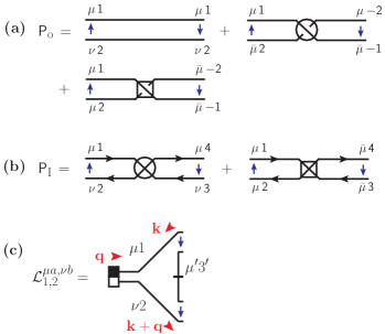
Figure 13: Feynman rules for class CI. (a) Disorder-only propagator $\mathsf{P}_{\mathrm{O}}$ in Eq. (159). The three diagrams represent the three terms (159a)–(159c) in respective order. We use blob and square nodes to distinguish spin exchange channels. (b) Interaction-dressed propagator $\mathsf{P}_{\mathrm{I}}$ in Eq. (159). The two diagrams represent the two terms (159d) and (159e) in respective order. (c) The stiffness vertex that arises from the coupling between fast and slow fields represented by Eq. (134).

Via the procedure leading to Eq. (130a), the propagators of the $\hat{W}_{\mathrm{j}=0,1,2,3}$ fields are readily obtained:

$$\left\langle[W_{0}]_{1,2}^{a,b}(-\mathbf{k})\,[W_{0}]_{3,4}^{c,d}({\bf k})\right\rangle= \,\mathsf{P}_{0,\lambda}+\tilde{\mathsf{P}}_{0,\lambda}+\mathsf{P}_{\mathrm{c}},$$ (156a)

$$\left\langle[W_{\alpha}]_{1,2}^{a,b}(-\mathbf{k})\,[W_{\alpha}]_{3,4}^{c,d}({\bf k})\right\rangle= \,\mathsf{P}_{\lambda}+\tilde{\mathsf{P}}_{\lambda}+\mathsf{P}_{\mathrm{s}},$$ (156b)

where the disorder-only components are

$$\mathsf{P}_{0,\lambda}= \,-\frac{1}{2}(1-\delta_{ab}\delta_{1,-2})\delta_{1,4}\delta_{2,3}\delta_{ad}\delta_{bc}\,\Delta_{\mathrm{O}}(|\omega_{1}|,|\omega_{2}|,\mathbf{k}),$$ (157a)

$$\tilde{\mathsf{P}}_{0,\lambda}= \,\frac{1}{2}(1-\delta_{ab}\delta_{1,-2})\delta_{1,-3}\delta_{2,-4}\,\delta_{ac}\delta_{bd}\,\Delta_{\mathrm{O}}(|\omega_{1}|,|\omega_{2}|,\mathbf{k}),$$ (157b)

$$\mathsf{P}_{\lambda}= \,\frac{1}{2}\delta_{1,4}\delta_{2,3}\delta_{ad}\delta_{bc}\,\Delta_{\mathrm{O}}(|\omega_{1}|,|\omega_{2}|,\mathbf{k}),$$ (157c)

$$\tilde{\mathsf{P}}_{\lambda}= \,\frac{1}{2}\delta_{1,-3}\delta_{2,-4}\delta_{ac}\delta_{bd}\,\Delta_{\mathrm{O}}(|\omega_{1}|,|\omega_{2}|,\mathbf{k}),$$ (157d)

and the interaction-dressed components are

$$\mathsf{P}_{\mathrm{c}}= \,2\Gamma_{\mathrm{c}}(s_{1}+s_{2})(s_{3}+s_{4})\delta_{1+3,2+4}$$

$$\times\delta_{ab}\delta_{bc}\delta_{cd}\frac{\Delta_{\mathrm{O}}(|\omega_{1}|,|\omega_{2}|,\mathbf{k})\,\Delta_{\mathrm{O}}(|\omega_{3}|,|\omega_{4}|,\mathbf{k})}{1+\gamma_{\mathrm{c}}f(|\omega_{1}-\omega_{2}|,{\bf k},\Lambda)},$$ (157e)

$$\mathsf{P}_{\mathrm{s}}= \,-2\Gamma_{\mathrm{s}}(s_{1}-s_{2})(s_{3}-s_{4})\delta_{1+3,2+4}$$

$$\times\delta_{ab}\delta_{bc}\delta_{cd}\Delta_{\mathrm{S}}(|\omega_{1}-\omega_{2}|,\mathbf{k})\,\Delta_{\mathrm{O}}(|\omega_{1}-\omega_{2}|,0,\mathbf{k}),$$ (157f)

with the diffusion kernels $\Delta_{\mathrm{O}}(|\omega_{1}|,|\omega_{2}|,\mathbf{k})$ and $\Delta_{\mathrm{S}}(|\omega|,\mathbf{k})$ and the logarithmic function $f(|\omega|,{\bf k},\Lambda)$ defined by Eqs. (131a), (131b), and (133), respectively. Similarly to the situation in class DIII, the propagators of the antisymmetric field $\hat{W}_{0}$ possess vanishing diagonal terms.

Via Eqs. (152), (156), and (157) we obtain the propagators of the $\hat{Y}$ fields:

$$\left\langle Y_{1,2}^{\mu a,\mu^{\prime}b}(-\mathbf{k})\,Y_{3,4}^{\nu c,\nu^{\prime}d}({\bf k})\right\rangle=\mathsf{P}_{\mathrm{O}}+\mathsf{P}_{\mathrm{I}}.$$ (158a)

$\mathsf{P}_{\mathrm{O}}$ and $\mathsf{P}_{\mathrm{I}}$ can be organized to the following forms that exhibit distinguished spin exchange channels:

$$\mathsf{P}_{\mathrm{O}}= \,\frac{1}{2}\left[\delta_{\mu^{\prime}\mu}\delta_{\nu^{\prime}\nu}\delta_{\mu\nu}\left(\mathsf{P}_{\lambda}-\mathsf{P}_{0,\lambda}\right)+2\delta_{\mu^{\prime}\bar{\mu}}\delta_{\nu^{\prime}\bar{\nu}}\delta_{\nu\mu^{\prime}}\mathsf{P}_{\lambda}\right]$$ (159a)

$$+\delta_{\mu^{\prime}\bar{\mu}}\delta_{\nu^{\prime}\bar{\nu}}\delta_{\nu\mu^{\prime}}\tilde{\mathsf{P}}_{\lambda}$$ (159b)

$$-\frac{1}{2}\delta_{\mu^{\prime}\mu}\delta_{\nu^{\prime}\nu}\delta_{\mu\bar{\nu}}\left(\tilde{\mathsf{P}}_{\lambda}+\tilde{\mathsf{P}}_{0,\lambda}\right),$$ (159c)

$$\mathsf{P}_{\mathrm{I}}= \,\frac{1}{2}\left[\delta_{\mu^{\prime}\mu}\delta_{\nu^{\prime}\nu}\delta_{\mu\nu}\left(\mathsf{P}_{\mathrm{s}}-\mathsf{P}_{\mathrm{c}}\right)+2\delta_{\mu^{\prime}\bar{\mu}}\delta_{\nu^{\prime}\bar{\nu}}\delta_{\nu\mu^{\prime}}\mathsf{P}_{\mathrm{s}}\right]$$ (159d)

$$-\frac{1}{2}\delta_{\mu^{\prime}\mu}\delta_{\nu^{\prime}\nu}\delta_{\mu\bar{\nu}}\left(\mathsf{P}_{\mathrm{s}}+\mathsf{P}_{\mathrm{c}}\right)$$ (159e)

where the barred spin index $\bar{\mu}$ is the “spin flip” of index $\mu$; e.g., $\{\mu,\bar{\mu}\}=\{\uparrow,\downarrow\}$.

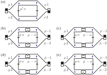
Figure 14: Category $\mathfrak{D}_{\text{CI}}1$: Disorder-only (weak localization) diagrams renormalizing $\lambda$ in class CI. The sum of the diagrams (b)–(e) gives the same contribution as (a). Summation is implied over repeated spin indices. The amplitude is evaluated in Eq. (160).

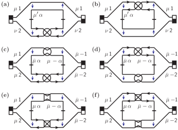
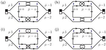
Figure 15: Category $\mathfrak{D}_{\text{CI}}2$: Interaction-dressed (Altshuler-Aronov) diagrams renormalizing $\lambda$ in class CI. The diagrams in the left and right columns give identical contributions. Moreover, the sum of the diagrams (c), (e), (g), and (i) gives the same contribution as (a). Summation is implied over repeated spin indices. The amplitude is evaluated in Eq. (161).

We represent the three terms (159a)-(159c) by the three diagrams in Fig. 13(a) in respective order. We note that the term (159a) preserves spin indices along the fermion lines, and (159b) and (159c) possess spin flips where the blob and square nodes distinguish spin exchange channels “$\mu\bar{\mu}\to\mu\bar{\mu}$” and “$\mu\mu\to\bar{\mu}\bar{\mu}$,” respectively. Similarly, the two terms (159d) and (159e) of the interaction-dressed propagator $\mathsf{P}_{\mathrm{I}}$ are represented by the two diagrams in Fig. 13(b). We use the blob and square nodes to distinguish spin exchange channels.

The stiffness vertex takes the form in Eq. (134) albeit involves extra spin indices, as depicted in Fig. 13(c). Via the symplectic condition (111b) one can show that the stiffness vertex matrix $\hat{\mathcal{L}}$ defined by Eq. (134b) satisfies constraints in spin space $\hat{\mathcal{L}}_{\mu\mu}=-\hat{\Sigma}^{1}\hat{\mathcal{L}}_{\bar{\mu}\bar{\mu}}^{\mathsf{T}}\hat{\Sigma}^{1}$ and $\hat{\mathcal{L}}_{\mu\bar{\mu}}=\hat{\Sigma}^{1}\hat{\mathcal{L}}_{\bar{\mu}\mu}^{\mathsf{T}}\hat{\Sigma}^{1}$, which is useful for evaluating the amplitudes of Feynman diagrams as discussed below.

(ii) Renormalization of $\lambda$. Diagrams $\mathfrak{D}_{\text{CI}}1$(a)–(e) appearing in Fig. 14 represent the weak-localization corrections to spin resistance $\lambda$ with amplitude

$$\begin{split}\sum_{\mathfrak{d}=\text{a}}^{\text{e}}\mathfrak{D}_{\text{CI}}1(\mathfrak{d})=&\,(nN+1)F\int_{\mathbf{r}}\text{Tr}(\nabla\hat{Q}_{\mathsf{S}}^{\dagger}\cdot\nabla\hat{Q}_{\mathsf{S}}).\end{split}$$ (160)

Diagrams $\mathfrak{D}_{\text{CI}}2$(a)-(j) appearing in Fig. 15 represent the Altshuler-Aronov correction to the spin resistance $\lambda$ with amplitude

$$\begin{split}&\sum_{\mathfrak{d}=\text{a}}^{\text{j}}\mathfrak{D}_{\text{CI}}2(\mathfrak{d})\\ &=\,F\left\{3\left[1+\frac{1-\gamma_{s}}{\gamma_{s}}\ln(1-\gamma_{s})\right]-\frac{1}{4}\mathcal{K}(\gamma_{\mathrm{c}})\right\}\\ &\quad\times\int_{\mathbf{r}}\text{Tr}(\nabla\hat{Q}_{\mathrm{S}}^{\dagger}\cdot\nabla\hat{Q}_{\mathrm{S}}).\end{split}$$ (161)

(iii) Full one-loop RG equations. Substituting $l_{\phi}=1$ [Eq. (108)] into Eqs. (160) and (161) and rescaling as in Eq. (139), we obtain the full one-loop RG equations:

$$\frac{\mathrm{d}\lambda}{\mathrm{d}\ell}= \,\lambda^{2}\left[1-(K\lambda)^{2}\right][1+\mathcal{J}(\gamma_{\mathrm{s}},\gamma_{\mathrm{c}})],$$ (162a)

$$\frac{\mathrm{d}\gamma_{\mathrm{s}}}{\mathrm{d}\ell}= \,-\frac{\lambda}{2}\gamma_{\mathrm{c}}(1-\gamma_{\mathrm{s}})(1-2\gamma_{\mathrm{s}}),$$ (162b)

$$\frac{\mathrm{d}\gamma_{\mathrm{c}}}{\mathrm{d}\ell}= \,\frac{\lambda}{2}\left\{-3\gamma_{\mathrm{s}}-2\gamma_{\mathrm{c}}+3\gamma_{\mathrm{c}}\left[\ln{(1-\gamma_{\mathrm{s}})}+\gamma_{\mathrm{s}}\right]\right\}-\gamma_{\mathrm{c}}^{2},$$ (162c)

where

$$\mathcal{J}(\gamma_{\mathrm{s}},\gamma_{\mathrm{c}})=3\left[1+\frac{1-\gamma_{\mathrm{s}}}{\gamma_{\mathrm{s}}}\ln{(1-\gamma_{\mathrm{s}})}\right]-\frac{1}{4}\mathcal{K}(\gamma_{\mathrm{c}}),$$ (163)

is the Altshuler-Aronov correction to the spin resistance $\lambda$. Equations (162b) and (162c) have been obtained in Ref. dellanna2006 and are valid to the lowest nontrivial order in $\lambda$ and $\gamma_{\mathrm{c}}$. The implications of Eq. (162) for the stability of class CI surface states were discussed in Refs. FXCup ; Foster2012 .

- (1) X.-L. Qi and S.-C. Zhang, Rev. Mod. Phys. 83, 1057 (2011).
- (2) J. H. Bardarson, J. Tworzydlo, P. W. Brouwer, and C. W. J. Beenakker, Phys. Rev. Lett. 99, 106801 (2007).
- (3) K. Nomura, M. Koshino, and S. Ryu, Phys. Rev. Lett. 99, 146806 (2007).
- (4) P. M. Ostrovsky, I. V. Gornyi, and A. D. Mirlin, Phys. Rev. Lett. 105, 036803 (2010).
- (5) A critical conductance is possible in a 3D topological insulator with long-ranged Coulomb interactions, doped away from the surface Dirac point. The precise nature of the surface state physics with disorder and interactions is not presently known, as it is predicted to arise in a perturbatively inaccessible strong coupling limit QGM2010 .
- (6) M. Z. Hasan and C. L. Kane, Rev. Mod. Phys. 82, 3045 (2010).
- (7) A. P. Schnyder, S. Ryu, A. Furusaki, and A. W. W. Ludwig, Phys. Rev. B 78, 195125 (2008).
- (8) A. Kitaev, AIP Conf. Proc. 1134, 22 (2009).
- (9) S. Ryu, A. P. Schnyder, A. Furusaki, and A. W. W. Ludwig, New J. Phys. 12, 065010 (2010).
- (10) M. S. Foster and E. A. Yuzbashyan, Phys. Rev. Lett. 109, 246801 (2012).
- (11) M. S. Foster, H.-Y. Xie, and Y.-Z. Chou, Phys. Rev. B 89, 155140 (2014).
- (12) A. W. W. Ludwig, M. P. A. Fisher, R. Shankar, and G. Grinstein, Phys. Rev. B 50, 7526 (1994).
- (13) A. M. Tsvelik, Phys. Rev. B 51, 9449 (1995).
- (14) P. M. Ostrovsky, I. V. Gornyi, and A. D. Mirlin, Phys. Rev. B 74, 235443 (2006).
- (15) B. L. Altshuler and A. G. Aronov, in Electron-Electron Interactions in Disordered Systems, edited by A. L. Efros and M. Pollak (North-Holland, Amsterdam, 1985).
- (16) I. L. Aleiner, B. L. Altshuler, and M. E. Gershenson, Waves Random Media 9, 201 (1999).
- (17) G. Zala, B. N. Narozhny, and I. L. Aleiner, Phys. Rev. B 64, 214204 (2001).
- (18) A. M. Finkel’stein, Zh. Eksp. Teor. Fiz. 84, 168 (1983) [Sov. Phys. JETP 57, 97 (1983)].
- (19) For a review, see D. Belitz and T. R. Kirkpartrick, Rev. Mod. Phys. 66, 261 (1994).
- (20) T. Senthil and M. P. A. Fisher, Phys. Rev. B 61, 9690 (2000).
- (21) K. Nomura, S. Ryu, A. Furusaki, and N. Nagaosa, Phys. Rev. Lett. 108, 026802 (2012).
- (22) R. Nakai and K. Nomura, Phys. Rev. B 89, 064503 (2014).
- (23) F. Evers and A. D. Mirlin, Rev. Mod. Phys. 80, 1355 (2008).
- (24) M. Jeng, A. W. W. Ludwig, T. Senthil, and C. Chamon, Bull. Am. Phys. Soc. 46, 231 (2001) (arXiv:cond-mat/0112044).
- (25) M. Fabrizio, L. Dell’Anna, and C. Castellani, Phys. Rev. Lett. 88, 076603 (2002).
- (26) L. Dell’Anna, Nucl. Phys. B 758, 255 (2006).
- (27) M. S. Foster and A. W. W. Ludwig, Phys. Rev. B 74, 241102(R) (2006); ibid. 77, 165108 (2008).
- (28) G. Catelani and I. L. Aleiner, Zh. Eksp. Teor. Fiz. 127, 372 (2005) [Sov. Phys. JETP 100, 331 (2005)].
- (29) L. Fu and E. Berg, Phys. Rev. Lett. 105, 097001 (2010).
- (30) K. Yada, M. Sato, Y. Tanaka, and T. Yokoyama, Phys. Rev. B 83, 064505 (2011).
- (31) A. Yamakage, K. Yada, M. Sato, and Y. Tanaka, Phys. Rev. B 85, 180509(R) (2012).
- (32) D. Bernard and A. LeClair, J. Phys. A: Math. Gen. 35, 2555 (2002).
- (33) In the microscopic model presented in Sec. III, it can be shown that the long-wavelength electric charge density appears as a Cartan subalgebra component of the non-abelian color current at the TSC surface.
- (34) The generate Sp(), SU(), and SO() color space algebras in classes CI, AIII, and DIII, respectively FXCup .
- (35) J. Tworzydlo, B. Trauzettel, M. Titov, A. Rycerz, and C. W. J. Beenakker, Phys. Rev. Lett. 96, 246802 (2006).
- (36) S. Ryu, C. Mudry, A. Furusaki, and A. W. W. Ludwig, Phys. Rev. B 75, 205344 (2007).
- (37) M. Müller, M. Bräuninger, and B. Trauzettel, Phys. Rev. Lett. 103, 196801 (2009).
- (38) E. Witten, Comm. Math. Phys. 92, 455 (1984).
- (39) S. Ryu, J. E. Moore, and A. W. W. Ludwig, Phys. Rev. B 85, 045104 (2012).
- (40) M. Stone, Phys. Rev. B 85, 184503 (2012).
- (41) P. M. Ostrovsky, I. V. Gornyi, and A. D. Mirlin, Phys. Rev. Lett. 98, 256801 (2007).
- (42) K. Nomura, S. Ryu, M. Koshino, C. Mudry, and A. Furusaki, Phys. Rev. Lett. 100, 246806 (2008).
- (43) Y.-Z. Chou and M. S. Foster, Phys. Rev. B 89, 165136 (2014).
- (44) Z. Wang, M. P. A. Fisher, S. M. Girvin, and J. T. Chalker, Phys. Rev. B 61, 8326 (2000).
- (45) C. Mudry, C. Chamon, and X.-G. Wen, Nucl. Phys. B 466, 383 (1996).
- (46) J. S. Caux, I. I. Kogan, and A. M. Tsvelik, Nucl. Phys. B 466, 444 (1996).
- (47) L. Fidkowski, X. Chen, and A. Vishwanath, Phys. Rev. X 3, 041016 (2013).
- (48) C. Wang, A. C. Potter, and T. Senthil, Science 343, 629 (2014).
- (49) C. Wang and T. Senthil, Phys. Rev. B 89, 195124 (2014).
- (50) M. A. Metlitski, L. Fidkowski, X. Chen, and A. Vishwanath, arXiv:1406.3032 (unpublished).
- (51) M. Sato, Phys. Rev. B 73, 214502 (2006).
- (52) B. Béri, Phys. Rev. B 81, 134515 (2010).
- (53) A. P. Schnyder and S. Ryu Phys. Rev. B 84, 060504(R) (2011); S. Matsuura, P.-Y. Chang, A. P. Schnyder, and S. Ryu, New. J. Phys. 15, 065001 (2013).
- (54) Y. X. Zhao and Z. D. Wang, Phys. Rev. Lett. 110, 240404 (2013); Phys. Rev. B 89, 075111 (2014).
- (55) A. P. Schnyder, S. Ryu, and A. W. W. Ludwig, Phys. Rev. Lett. 102, 196804 (2009).
- (56) N. W. Ashcroft and N. D. Mermin, Solid State Physics (Saunders College, Philadelphia, 1976), p. 69.
- (57) R. Jackiw and C. Rebbi, Phys. Rev. D 13, 3398 (1976).
- (58) G. D. Mahan, Many-Particle Physics 3rd ed. (Kluwer Academic/Plenum, New York, 2000).
- (59) For Ward identities in Matsubara frequencies see p. 514 of Ref. SUP-mahanbook, .
- (60) A. Kashuba, Phys. Rev. B 78, 085415 (2008).
- (61) L. Fritz, J. Schmalian, M. Müller, and S. Sachdev, Phys. Rev. B 78, 085416 (2008); M. Müller, L. Fritz, and S. Sachdev, ibid. 78, 115406 (2008); M. Müller and S. Sachdev, ibid. 78, 115419 (2008).
- (62) M. S. Foster and I. L. Aleiner, Phys. Rev. B 79, 085415 (2009).
- (63) A. Altland and B. Simons, Condensed Matter Field Theory, 2nd. Ed. (Cambridge University Press, Cambridge, 2010).
- (64) A. A. Nersesyan, A. M. Tsvelik, and F. Wegner, Phys. Rev. Lett. 72, 2628 (1994).
- (65) R. Gade and F. Wegner, Nucl. Phys. B 360, 213 (1991); R. Gade, ibid. 398, 499 (1993).
- (66) For class DIII we exploit the formula for .