Simulation of multivariate diffusion bridges

Abstract

We propose simple methods for multivariate diffusion bridge simulation, which plays a fundamental role in simulation-based likelihood and Bayesian inference for stochastic differential equations. By a novel application of classical coupling methods, the new approach generalizes a previously proposed simulation method for one-dimensional bridges to the multi-variate setting. First a method of simulating approximate, but often very accurate, diffusion bridges is proposed. These approximate bridges are used as proposal for easily implementable MCMC algorithms that produce exact diffusion bridges. The new method is much more generally applicable than previous methods. Another advantage is that the new method works well for diffusion bridges in long intervals because the computational complexity of the method is linear in the length of the interval. In a simulation study the new method performs well, and its usefulness is illustrated by an application to Bayesian estimation for the multivariate hyperbolic diffusion model.

Key words: Bayesian inference; coupling; discretely sampled diffusions; likelihood inference; stochastic differential equation; time-reversal.

Address for correspondance: Michael Sørensen, Dept. of Mathematical Sciences, University of Copenhagen, Universitetsparken 5, DK-2100 Copenhagen Ø, Denmark.
E-mail: michael@math.ku.dk

1 Introduction

In this paper we propose a simple and generally applicable method for simulation of a multi-variate diffusion bridge. The main motivation is that simulation of diffusion bridges plays a fundamental role in simulation-based likelihood inference (including Bayesian inference) for discretely sampled diffusion processes and other diffusion-type processes like stochastic volatility models.

Our approach is based on the following simple construction of a process that starts from $a$ at time zero and at time $T$ ends in $b$, where $a$ and $b$ are given points in the state space. One diffusion process, $X^{(1)}_{t}$, is started from the point $a$, while another diffusion, $X^{(2)}_{t}$ is started from the point $b$. The time of the second diffusion is reversed, so that the time starts at $T$ and goes downwards to zero, and the dynamics of $X^{(2)}_{t}$ is chosen such that the time reversed diffusion $X^{(2)}_{T-t}$ has the same dynamics as $X^{(1)}_{t}$. Suppose there is a time point $\tau\in[0,T]$ at which $X^{(1)}_{\tau}=X^{(2)}_{T-\tau}$. Then the process that is equal to $X^{(1)}_{t}$ for $t\in[0,\tau]$ and for $t\in[\tau,T]$ equals $X^{(2)}_{T-t}$ is obviously a process that starts at $a$ and ends at $b$. If the two diffusion processes $X^{(1)}$ and $X^{(2)}$ are independent, then the probability that $X^{(1)}_{t}$ and $X^{(2)}_{T-t}$ meet at the same time point in $[0,T]$ is zero for dimensions larger than one. However, if they are suitably dependent, then the probability can be made positive and will often go to one as $T$ tends to infinity. This can be obtained by applying classical coupling methods.

The new method is a generalization of the one-dimensional diffusion bridge simulation method proposed by Bladt and Sørensen (2014), where the two diffusions $X^{(1)}$ and $X^{(2)}$ were independent. The generalization is far from straightforward. For ergodic one-dimensional diffusions, the probability that two independent diffusions intersect goes to one as $T\rightarrow\infty$. The application of coupling methods is a breakthrough that allows the generalization to multivariate diffusions. Moreover, the coupling methods also improve the simulation of one-dimensional diffusions because they increase the probability of intersection in $[0,T]$ and thus improve the computational efficiency of the method.

Conditional on the event that the two processes meet at a time point in $[0,T]$, we show that the process constructed as described above is an approximation to a diffusion bridge between the two points. A simple rejection sampler is obtained by repeatedly simulating the two dependent diffusions until they hit each other. The diffusions can be simulated by means of simple procedures like the Euler or the Milstein scheme, see Kloeden and Platen (1999), so the new method is easy to implement for likelihood inference for discretely sampled diffusion processes. The approximate diffusion bridge produced by the rejection sampler can be used as proposal for MCMC-algorithms that have an exact diffusion bridge as target distribution. We present a pseudo-marginal Metropolis-Hastings algorithm (in the sense of Andrieu and Roberts (2009)) and a new MCMC algorithm that is easier to implement, but typically has a larger rejection probability. An example of a diffusion bridge simulated by our new method is shown in Figure 1.1.

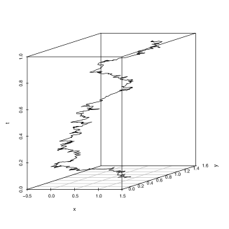
Figure 1.1: Simulated sample path of an Ornstein-Uhlenbeck bridge from (0.785,0.785) to (1.091,1.091). Time is in the vertical direction.

Diffusion bridge simulation is a highly non-trivial problem that has been investigated actively over the last 10 - 15 years. A lucid exposition of the problems and the state-of-the-art can be found in Papaspiliopoulos and Roberts (2012). Before the paper by Bladt and Sørensen (2014), it was thought impossible to simulate diffusion bridges by means of simple procedures, because a rejection sampler that tries to hit the prescribed end-point for the bridge will have a prohibitively large rejection probability. The rejection sampler presented in this paper has an acceptable rejection probability because what must be hit is a sample path rather than a point and because the coupling methods make the two diffusions tend to meet. The first diffusion bridge simulation methods in the literature were based on the Metropolis-Hastings algorithm with a proposal distribution given by a diffusion process that was forced by its drift to go from $a$ to $b$, see e.g. Roberts and Stramer (2001) or Durham and Gallant (2002). Later Beskos et al. (2006b, 2008) developed algorithms for exact simulation of diffusion bridges. These are cleverly designed rejection sampling algorithms that use simulations of Brownian bridges, which can easily be simulated. Under strong boundedness conditions the algorithm is relatively simple, whereas it is more complex under weaker condition. Lin et al. (2010) proposed a sequential Monte Carlo method for simulating diffusion bridges with a resampling scheme guided by the empirical distribution of backward paths. The spirit of this approach has similarities to the methods in Bladt and Sørensen (2014) and in this paper.

An advantage of our new method is that the same simple algorithm can be used for all ergodic diffusions, and that it is easy to understand and to implement. More importantly, the method does not require that the diffusion can be transformed into one with diffusion matrix equal to the identity matrix. Such a transformation, often referred to as the Lamperti transformation, exists for only a small subclass of the multi-variate diffusions, and even when it exists, the transformation is rarely in closed form. A Lamperti transformation is required for the exact algorithms of Beskos et al. (2006b, 2008). Another important advantage is that our method works particularly well for long time intervals. The computational complexity is linear in the length of the time interval where the diffusion bridge is defined. This was illustrated in a simulation study in Bladt and Sørensen (2014), where the computer time increased linearly with the interval length for our method, while it grew at least exponentially with the interval length for the exact EA algorithms of Beskos et al. (2006b). The latter finding is not surprising, because in the fundamental EA1 algorithm the acceptance probability is of the order $e^{-cT}$, where $T$ is the length of the interval. Thus the EA algorithm is in practice likely not to work for long time intervals. It follows from results in this paper that under conditions given in the literature on coupling of diffusion processes (see Chen and Li (1989)), the approximate method proposed here simulates an essentially exact diffusion bridge in long time intervals (apart from the discretization error). This literature also gives conditions ensuring that the distribution of the simulated process goes to that of a diffusion bridge exponentially fast as a function of the interval length. Thus the proposed method usefully supplements previously published methods both because it works particularly well for long time intervals, where the other methods tend not to work, and because it works for diffusions without a Lamperti transformation. It is worth noting that simulation-based likelihood inference for discretely sampled diffusions is mainly important for long time intervals, because for short time intervals several simpler methods provide highly efficient estimators, see the following discussion.

The main challenge in likelihood based inference for diffusion models is that the transition density, and hence the likelihood function, is not explicitly available and must therefore be approximated. When the sampling frequency is relatively high, rather crude approximations to the likelihood functions, like those in Ozaki (1985), Bollerslev and Wooldridge (1992), Bibby and Sørensen (1995) and Kessler (1997), give estimators with a high efficiency, see Sørensen (2010). When the interval between the observation times is relatively long, more accurate approximations to the transition density are needed. One approach is numerical approximations, either by solving the Kolmogorov PDE numerically, e.g. Poulsen (1999) and Hurn et al. (2007), or by expansions, e.g. Aït-Sahalia (2002, 2008) and Forman and Sørensen (2008). Alternatively, likelihood inference can be based on simulations, an approach that goes back to the seminal paper by Pedersen (1995). The inference problem can be viewed as an incomplete data problem. If the diffusion process had been observed continuously, the likelihood functions would be explicitly given by the Girsanov formula. However, the process has been observed at discrete time points only, and the continuous-time paths between the observation points can be considered as missing data. This way of viewing the problem, which goes back to Dacunha-Castelle and Florens-Zmirou (1986), makes it natural to apply either the EM-algorithm or the Gibbs sampler. To do so the missing continuous paths between the observations must be simulated conditional on the observations, which by the Markov property is exactly simulation of diffusion bridges. It was a significant break-through when this was simultaneously realized by several authors, see Roberts and Stramer (2001), Elerian et al. (2001), Eraker (2001), and Durham and Gallant (2002), and approaches based on bridge simulation has since been used by several authors including Golightly and Wilkinson (2005, 2006, 2011), Beskos et al. (2006a), Delyon and Hu (2006), Beskos et al. (2009), and Lin et al. (2010).

Diffusion bridge simulation is also crucial to simulation-based inference for other types of diffusion process data than discrete time observations. Chib et al. (2006) presented a general approach to simulation-based Bayesian inference for diffusion models when the data are discrete time observations of rather general, and possibly random, functionals of the continuous sample path, see also Golightly and Wilkinson (2008). This approach covers for instance diffusions observed discretely with measurement error and discretely sampled stochastic volatility models. Also in this case diffusion bridge simulation is crucial. Baltazar-Larios and Sørensen (2010) presented an EM-algorithm for integrated diffusions observed discretely with measurement error based on the ideas in Chib et al. (2006) and the bridge simulation method proposed in Bladt and Sørensen (2014).

The paper is organized as follows. In Section 2 we first review some necessary results on coupling methods and time-reversal for diffusion processes and prove some preliminary results. Then we present the new approximate bridge simulation method and show in what sense it approximates a diffusion bridge. The approximate bridges are then used as proposal in two MCMC-algorithms that have an exact diffusion bridge as target distribution. Finally, we discuss how the new method improves simulation of one-dimensional diffusions and solve some implementation problems. In particular, we give criteria to determine whether two diffusions simulated at discrete time points have met between two time points. In Section 3 the approximate and exact bridge simulation methods are compared to the (known) exact distribution of the multivariate Ornstein–Uhlenbeck bridge. The study indicates that our approximate method provides a very accurate approximation to the distribution of a diffusion bridge, except for bridges that are unlikely to occur in discretely sampled data. Even for extremely unlikely bridges, the approximate method works surprisingly well for some coupling methods. In Section 4 we illustrate the usefulness of our method to inference for discretely observed diffusions by considering briefly Bayesian estimation for the multivariate hyperbolic diffusion. The proofs are collected in Section 5.

2 Diffusion bridge simulation

Let $X=\{X_{t}\}_{t\geq 0}$ be a $d$-dimensional diffusion with state space $D$ given by the stochastic differential equation

$$dX_{t}=\alpha(X_{t})dt+\sigma(X_{t})dW_{t},$$ (2.1)

where $W$ is a $d$-dimensional Wiener process, and where the coefficients $\alpha$ (a function $D\mapsto{\rm I\mkern-2.5mu\nonscript\mkern-0.5muR}^{d}$) and $\sigma$ (a $d\times d$-matrix of continuous functions defined on $D$) are sufficiently regular to ensure that the equation has a unique strong solution that is a strong Markov process. We will assume that the diffusion defined by (2.1) is ergodic with invariant probability density function $\nu$ (w.r.t. Lebesgue measure on $D$). It is assumed that $\sigma(x)$ is invertible for all $x\in D$. Define $V(x)=\sigma(x)\sigma(x)^{T}$. We denote the transition density of $X$ by $p_{t}(x,y)$. Specifically, the conditional density of $X_{s+t}$ given $X_{s}=x$ is $y\mapsto p_{t}(x,y)$.

Let $a$ and $b$ be given points in $D$. We present a method for simulating a sample path of $X$ in $[0,T]$ such that $X_{0}=a$ and $X_{T}=b$. A solution of (2.1) in the interval $[0,T]$ such that $X_{0}=a$ and $X_{T}=b$ will in the following be called an $(a,b,T)$-bridge. The approximate bridge construction goes as follows. First the time-reversed version, $X^{*}_{t}$, of (2.1) is simulated in $[0,T]$ starting at $b$. Then a solution, $X_{t}$, to (2.1) is simulated starting at $a$ and dependent on $X^{*}$ in such a way that $X_{t}$ and $X^{*}_{T-t}$ tend to intersect at some (random) time point $\tau\in[0,T]$. If the two processes meet at time $\tau$, then the approximate bridge is the equal to $X_{t}$ for $t\in[0,\tau]$, and equal to $X^{*}_{T-t}$ for $t\in[\tau,T]$. This approximate bridge is used as a proposal for a MCMC algorithm that has the exact $(a,b,T)$-bridge as target distribution. The required dependence between $X^{*}$ and $X$ is obtained by applying classical coupling methods for diffusions.

2.1 Coupling and time-reversal for multivariate diffusions

We present our algorithm for a class of coupling methods that includes the coupling by reflection method of Lindvall and Rogers (1986) and the coupling by projection by Chen and Li (1989). Other coupling methods (see e.g. Chen and Li (1989)) can be used similarly, provided that they couple before time $T$ with a probability that is not too small. We begin by briefly presenting the class of coupling methods. Then we derive a few results that we need in order to construct diffusion bridges.

Suppose $X$ solves (2.1) with initial value $X_{0}=x_{0}$. Define another diffusion process $X^{\prime}$ as the solution to

$$dX^{\prime}_{t}=\alpha(X^{\prime}_{t})dt+\sigma(X^{\prime}_{t})dW^{\prime}_{t},\ \ \ X^{\prime}_{0}=x^{\prime}_{0}$$ (2.2)

with the Wiener process

$$dW^{\prime}_{t}=\left\{I-(1-\gamma)\Pi(X_{t},X^{\prime}_{t})\right\}{\cal O}(X_{t},X^{\prime}_{t})dW_{t}+\sqrt{1-\gamma^{2}}u(X_{t},X^{\prime}_{t})dU_{t}.$$

Here $\gamma\in[-1,1)$, $U$ is a univariate standard Wiener process independent of $W$, $I$ is the $d$-dimensional identity matrix and

$$\Pi(x,x^{\prime})=u(x,x^{\prime})u(x,x^{\prime})^{T},$$ (2.3)

where $T$ denotes transposition, and $u(x,x^{\prime})$ is the unit vector such that $\sigma(x^{\prime})u(x,x^{\prime})$ points in the direction $x-x^{\prime}$, i.e.

$$u(x,x^{\prime})=\frac{\sigma(x^{\prime})^{-1}(x-x^{\prime})}{|\sigma(x^{\prime})^{-1}(x-x^{\prime})|}.$$

Finally, ${\cal O}(X_{t},X^{\prime}_{t})$ is an orthogonal matrix that in some cases is needed to ensures that the law of $(X,X^{\prime})$ does not depend on the particular choice of $\sigma$, but only on the law of the solution $X$ (the law of $X$ depends only on $\sigma\sigma^{T}$, so the same law can be obtained for many different choices of $\sigma$). For many stochastic differential equations, indeed for all those we consider in this paper, we have ${\cal O}=I$, but there may be cases where the choice of $\sigma$ introduces a rotation which should be counterbalanced. In fact, as long as $\sigma$ satisfies the smoothness requirements of Lindvall and Rogers (1986) and Chen and Li (1989) our method can still work if we choose ${\cal O}=I$ for reasons of computational efficiency. However, it may take many more attempts to achieve the successful coupling from which we construct our bridge. The matrix ${\cal O}(X_{t},X^{\prime}_{t})$ should be chosen to be the closest orthogonal matrix to $\sigma(X_{t})^{T}\sigma(X^{\prime}_{t})$ in the Frobenious norm. That is ${\cal O}(X_{t},X_{t}^{\prime})=AB^{T}$ where $\sigma(X_{t})^{T}\sigma(X^{\prime}_{t})=A\Sigma B^{T}$ is the singular value decomposition.

The matrix $\Pi(x,x^{\prime})$ is the orthogonal projection onto the one-dimensional subspace generated by the vector $u(x,x^{\prime})$, while $I-\Pi(x,x^{\prime})$ is projection onto the plane orthogonal to the vector $u(x,x^{\prime})$. Using this geometric interpretation, it is not difficult to see that the quadratic variation of $W^{\prime}$ equals $tI$ implying that $W^{\prime}$ is a Wiener process.

Consider the case where ${\cal O}=I$. In the plane orthogonal to the vector $u(X_{t},X^{\prime}_{t})$, the increment of the Wiener process $W^{\prime}$ is equal to the increment of $W$. In the direction $u(X_{t},X^{\prime}_{t})$, the increment of $W^{\prime}$ is equal to minus the increment of $W$ in the same direction (i.e. $\Pi(X_{t},X^{\prime}_{t})dW_{t}$) if $\gamma=-1$ (method of reflection). Otherwise, the increment of $W^{\prime}$ in the direction $u(X_{t},X^{\prime}_{t})$ is the sum of $\gamma\Pi(X_{t},X^{\prime}_{t})dW_{t}$ and $\sqrt{1-\gamma^{2}}u(X_{t},X^{\prime}_{t})dU_{t}$. In particular if $\gamma=0$, the increment of $W^{\prime}$ in the direction $u(X_{t},X^{\prime}_{t})$ it is equal to the increment of the independent Wiener process $U$ on the subspace generated by $u(X_{t},X^{\prime}_{t})$ (method of projection). For $\gamma=-1$, $dW^{\prime}_{t}=H(X_{t},X^{\prime}_{t}))dW_{t}$, where the matrix

$$H(x,x^{\prime})=I-2\Pi(x,x^{\prime})$$

is reflection in the plane orthogonal to the vector $u(x,x^{\prime})$. It is therefore symmetric and orthonormal. We do not consider the case $\gamma=1$ where (for ${\cal O}=I$) the two diffusions are driven by the same Wiener process and will not meet.

The squared diffusion coefficient of the $2d$-dimensional diffusion $(X_{t},X^{\prime}_{t})$ is

$$\left(\begin{array}[]{cc}\sigma(x)\sigma(x)^{T}&\sigma(x){\cal O}(x,x^{\prime})^{T}\left\{I-(1-\gamma)\Pi(x,x^{\prime}))\right\}\sigma(x^{\prime})^{T}\\ &\\ \sigma(x^{\prime})\left\{I-(1-\gamma)\Pi(x,x^{\prime}))\right\}{\cal O}(x,x^{\prime})\sigma(x)^{T}&\sigma(x^{\prime})\sigma(x^{\prime})^{T}\end{array}\right),$$

which is of the general form treated in Chen and Li (1989).

Define the stopping time

$$\tau=\inf\{t>0\,|\,X_{t}=X^{\prime}_{t}\}.$$ (2.4)

Lindvall and Rogers (1986), Chen and Li (1989) and others have given conditions on the coefficients $\alpha$ and $\sigma$ ensuring that $P(\tau<\infty)=1$. This is not really necessary for our bridge simulation method to work. The method is a rejection sampler with rejection probability $P(\tau>T)$, so we just need that this probability is not too large. If $P(\tau<\infty)=1$ that is certainly the case if $T$ is sufficiently large. Chen and Li (1989)) gave results on the rate of convergence of $P(\tau>T)$ to zero as $T\rightarrow\infty$, in particular conditions ensuring geometrically fast convergence. As these conditions are somewhat technical and unnecessarily restrictive for our application, they are not stated here.

Lemma 2.1

The sample path of $X^{\prime}$ in $[0,t]$ is a function of the sample path of $X$ in $[0,t]$, the initial value $x^{\prime}_{0}$, and the sample path of the one-dimensional Wiener process $U$ in $[0,t]$

$$\{X^{\prime}_{s}\}_{0\leq s\leq t}={\cal K}_{t}\left(x^{\prime}_{0},\{X_{s}\}_{0\leq s\leq t},\{U_{s}\}_{0\leq s\leq t}\right).$$

Specifically,

$$X^{\prime}_{s}=x^{\prime}_{0}+\int_{0}^{s}\alpha(X^{\prime}_{u})du+\int_{0}^{s}\sigma(X^{\prime}_{u})\{I-(1-\gamma)\Pi(X_{t},X^{\prime}_{t})\}{\cal O}(X_{t},X^{\prime}_{t})\sigma(X_{u})^{-1}dX_{u}$$ (2.5)

$$\mbox{}\hskip 42.67912pt-\int_{0}^{s}\sigma(X^{\prime}_{u})\{I-(1-\gamma)\Pi(X_{t},X^{\prime}_{t})\}{\cal O}(X_{t},X^{\prime}_{t})\sigma(X_{u})^{-1}\alpha(X_{u})du$$

$$\mbox{}\hskip 42.67912pt+\sqrt{1-\gamma^{2}}\int_{0}^{s}\sigma(X^{\prime}_{u})u(X_{t},X^{\prime}_{t})dU_{u}.$$

Similarly, the sample path of $X$ in $[0,t]$ is a function of the initial value $x_{0}$, the sample paths of $X^{\prime}$ in $[0,t]$, and the sample path in $[0,t]$ of a standard univariate Wiener process, $U^{\prime}$, independent of $X^{\prime}$

$$\{X_{s}\}_{0\leq s\leq t}=\tilde{\cal K}_{t}\left(x_{0},\{X^{\prime}_{s}\}_{0\leq s\leq t},\{U^{\prime}_{s}\}_{0\leq s\leq t}\right).$$

Specifically,

$$X_{s} = x_{0}+\int_{0}^{s}\alpha(X_{u})du+\int_{0}^{s}\sigma(X_{u}){\cal O}(X_{u},X^{\prime}_{u})^{T}\{I-(1-\gamma)\Pi(X_{u},X^{\prime}_{u})\}\sigma(X^{\prime}_{u})^{-1}dX^{\prime}_{u}$$ (2.6)

$$\mbox{}\hskip 42.67912pt-\int_{0}^{s}\sigma(X_{u}){\cal O}(X_{u},X^{\prime}_{u})^{T}\{I-(1-\gamma)\Pi(X_{u},X^{\prime}_{u})\}\sigma(X^{\prime}_{u})^{-1}\alpha(X^{\prime}_{u})du$$

$$\mbox{}\hskip 42.67912pt+\sqrt{1-\gamma^{2}}\int_{0}^{s}\sigma(X_{u}){\cal O}(X_{u},X^{\prime}_{u})^{T}u(X_{u},X^{\prime}_{u})dU^{\prime}_{u}.$$

Proofs of this and other results are given in Section 5. Note that for $\gamma=-1$, $\tilde{\cal K}_{t}$ does not depend on $U^{\prime}$.

Before we can formulate the main theorem on our method, we need to review some well-known results on time-reversal of multivariate diffusions. We have assumed that the diffusion $X$ defined by (2.1) is ergodic with invariant probability density function $\nu$. Hence a stationary version of $X$ exists. If the time is reversed for this stationary process, we obtain another stationary diffusion process $X^{*}$. By Theorem 2.3 in Millet et al. (1989), the time-reversed diffusion $X^{*}$ solves the stochastic differential equation

$$dX^{*}_{t}=\alpha^{*}(X^{*}_{t})dt+\sigma(X^{*}_{t})dW_{t}$$ (2.7)

where

$$\alpha_{i}^{*}(x)=-\alpha_{i}(x)+\nu(x)^{-1}\sum_{j=1}^{d}\partial_{x_{j}}\left(\nu(x)V(x)_{ij}\right),\ \ i=1,\ldots,d,$$ (2.8)

provided that

$$\int_{D}\left|\sum_{j=1}^{d}\partial_{x_{j}}\left(\nu(x)V_{ij}(x)\right)\right|dx<\infty,\ \ i=1,\ldots,d.$$ (2.9)

We assume that the local integrability condition (2.9) is satisfied. Conditions ensuring this are discussed in Millet et al. (1989), where also a similar result under the local Lipschitz condition is given. The condition (2.9) is satisfied if the two coefficients are twice continuously differentiable on $D$, and if there exists $\epsilon>0$ such that $V\geq\epsilon I$. Alternative conditions can be found in Haussmann and Pardoux (1986). In cases where the transition density is not differentiable with respect to $x$, the partial derivative in the formula for the drift are in the distributional sense.

Let $p^{*}_{t}(x,y)$ denote the transition density of the solution to (2.7). If $X$ is the stationary version of the solution to (2.1) and $X^{*}$ is the time-reversed stationary diffusion, then the distribution of $(X_{s},X_{s+t})$ equals the distribution of $(X^{*}_{s+t},X^{*}_{s})$. Hence

$$p_{t}(x,y)\nu(x)=p^{*}_{t}(y,x)\nu(y),$$ (2.10)

2.2 Approximate bridge simulation

In this subsection we present the mathematical results on which our algorithm to approximately simulate a diffusion bridge is based and describe how the results can be used to construct the algorithm. Detailed implementation questions are discussed in a later section.

Theorem 2.2

Suppose $X$ solves (2.1) for $t\in[0,T]$ with the initial condition $X_{0}\sim\nu$, where $\nu$ is the invariant probability measure. Let $X^{\prime}$ be the corresponding solution to (2.2) with initial condition $X^{\prime}_{0}=a$, i.e. $\{X^{\prime}_{t}\}_{0\leq t\leq T}={\cal K}_{T}\left(a,\{X_{s}\}_{0\leq t\leq T},\{U_{t}\}_{0\leq t\leq T}\right)$, where $U$ is a standard Wiener process independent of $X$. Define a process by

$$Z_{t}=\left\{\begin{array}[]{ll}X^{\prime}_{t}&\mbox{\rm if }\ 0\leq t\leq\tau\\ &\\ X_{t}&\mbox{\rm if }\ \tau<t\leq T,\end{array}\right.$$

where $\tau$ is given by (2.4).

Then the distribution of $\{Z_{t}\}_{0\leq t\leq T}$ conditional on the events $\tau\leq T$ and $X_{T}=b$ equals the distribution of a $(a,b,T)$-bridge, $B$, conditional on the event that the bridge is hit by the process $\tilde{\cal K}_{T}\left(A,\{B_{t}\}_{0\leq t\leq T},\{U^{\prime}_{t}\}_{0\leq t\leq T}\right)$. Here $A$ is a $d$-dimensional random variable with density function $p^{*}_{T}(b,\cdot)$ given by (2.10), $U^{\prime}$ is a standard univariate Wiener process, and $A$, $U^{\prime}$ and $B$ are independent.

We refer to the process $\tilde{\cal K}_{T}\left(A,\{B_{t}\}_{0\leq t\leq T},\{U^{\prime}_{t}\}_{0\leq t\leq T}\right)$ as the $p^{*}_{T}(b)$-diffusion associated with $B$. This process plays an important role not only in the characterization of the distribution of the approximate diffusion bridge $Z$, but also in the method for simulating exact diffusion bridges presented in the next subsection. When $\gamma=-1$, ${\cal K}_{T}$ does not depend on $U$ and $\tilde{\cal K}_{T}$ does not depend on $U^{\prime}$.

A sample path of $X$ with $X_{0}\sim\nu$ conditional on $X_{T}=b$ can easily be obtained by using the result of the following lemma on the distribution of a time-reversed diffusion started at the point $b$.

Lemma 2.3

Suppose $X$ is ergodic with invariant probability density function $\nu$, and let $X^{*}$ be a solution to (2.7) with initial condition $X^{*}_{0}=b$. Define the time-reversed process $\bar{X}_{t}=X^{*}_{T-t}$, $0\leq t\leq T$. The process $\{\bar{X}_{t}\}$ and the conditional process $\{X_{t}\}$ given that $X_{T}=b$ have the same transition densities

$$q(x,s,y,t)=\frac{p_{t-s}(x,y)p_{T-t}(y,b)}{p_{T-s}(x,b)}=\frac{p^{*}_{t-s}(y,x)p^{*}_{T-t}(b,y)}{p^{*}_{T-s}(b,x)},\hskip 14.22636pts<t<T.$$ (2.11)

The distribution of $\{\bar{X}_{t}\}$ is equal to the distribution of the process $\{X_{t}\}$ with $X_{0}\sim\nu$ conditional on $X_{T}=b$.

Based on Theorem 2.2 and Lemma 2.3 we can now propose an algorithm to simulate an approximate diffusion bridge in the interval $[0,T]$. Use any of the several methods available (see e.g. Kloeden and Platen (1999)) to simulate the diffusion $X^{*}$ given by (2.7) with $X^{*}_{0}=b$. If the diffusion given by (2.1) is time-reversible, then the stochastic differential equation for $X^{*}$ is simply (2.1). To simplify the exposition, we assume that $X^{*}$ has been simulated by means of the Euler-scheme with step size $\delta=T/N$. Let $Y^{*}_{\delta i}$, $i=0,1,\ldots,N$, denote the simulated values of the process, while $\Delta W_{i}=W_{\delta i}-W_{\delta(i-1)}$, $i=1,\ldots,N$, denote the simulated increments of the driving $d$-dimensional Wiener process, i.e. $Y^{*}_{0}=b$ and

$$Y^{*}_{\delta i}=Y^{*}_{\delta(i-1)}+\alpha^{*}(Y^{*}_{\delta(i-1)})\delta+\sigma(Y^{*}_{\delta(i-1)})\Delta W_{i},$$

$i=1,\ldots,N$. The increments of the Wiener process that drives the time-reversed version of $Y^{*}$ (i.e. $Y^{*\mbox{rev}}_{\delta i}=Y^{*}_{\delta(N-i)}$) are

$$\Delta W^{\mbox{rev}}_{i}=\sigma(Y^{*}_{\delta(N-i+1)})^{-1}\left(Y^{*}_{\delta(N-i)}-Y^{*}_{\delta(N-i+1)}-\alpha(Y^{*}_{\delta(N-i+1)})\delta\right).$$ (2.12)

For fine discretizations $\Delta W^{\mbox{rev}}_{i}\approx-\Delta W_{N-i+1}$.

The discretized sample path of $X^{\prime}$ is a function of the simulated process $Y^{*}$ and (except in the case of the method of reflection, $\gamma=-1$) an independent one-dimensional standard Wiener process $B$, the increments of which we denote by $\Delta B_{i}=B_{\delta i}-B_{\delta(i-1)}$, $i=1,\ldots,N$. If we denote the simulated values of $X^{\prime}$ by $Y^{\prime}_{\delta i}$, $i=0,1,\ldots,N$, we have that $Y^{\prime}_{0}=a$ and

$$Y^{\prime}_{\delta i}=Y^{\prime}_{\delta(i-1)}+\alpha(Y^{\prime}_{\delta(i-1)})\delta+\sigma(Y^{\prime}_{\delta(i-1)})\Delta W^{\prime}_{i},$$ (2.13)

$i=1,\ldots,N$, where

$$\Delta W^{\prime}_{i} = \left\{I-(1-\gamma)\Pi(Y^{*}_{\delta(N-i+1)},Y^{\prime}_{\delta(i-1)})\right\}{\cal O}(Y^{*}_{\delta(N-i+1)},Y^{\prime}_{\delta(i-1)})\Delta W^{\mbox{rev}}_{i}$$

$$\mbox{}\hskip 56.9055pt+\sqrt{1-\gamma^{2}}u(Y^{*}_{\delta(N-i+1)},Y^{\prime}_{\delta(i-1)})\Delta B_{i}.$$

A simulation of an approximation in the sense of Theorem 2.2 to a $(a,b,T)$-bridge is obtained by rejection sampling. Keep simulating independent copies of $Y^{*}$ and $B$ until there is an $i$ such that $Y^{*}_{\delta(T-i)}$ and $Y^{\prime}_{\delta i}$ are sufficiently close that we can safely assume that coupling happens in the time interval $[\delta i,\delta(i+1)]$. We discuss the problem of deciding whether coupling has happened or not in more detail in Subsection 2.5. Once coupling has been obtained (in the interval $[\delta i,\delta(i+1)]$), put $\rho=i+1$ and define

$$Z_{\delta i}=\left\{\begin{array}[]{ll}Y^{\prime}_{\delta i}&\mbox{\rm for }\ i=0,1,\ldots,\rho-1\\ &\\ Y^{*}_{\delta(N-i)}&\mbox{\rm for }\ i=\rho,\ldots N,\end{array}\right.$$ (2.15)

On top of the usual influence of the step size $\delta$ on the quality of the individual simulated trajectories, the step size also controls the probability that a trajectory crossing is not detected. Therefore, it is advisable to choose $\delta$ smaller than in usual simulation of diffusion sample paths. Another problem is that the method will only work, if $P(\tau\leq T)$ is not too small. This problem was considered in Lindvall and Rogers (1986) and Chen and Li (1989).

The results of Lemma 2.3 and Theorem 2.2, and hence the algorithm, simplify if the diffusion process is time reversible in the sense that $p^{*}_{t}(x,y)=p_{t}(x,y)$, or equivalently $p_{t}(x,y)\nu(x)=p_{t}(y,x)\nu(y)$. Diffusions with the latter property are called $\nu$-symmetric, see Kent (1978). By equating $\alpha$ to the reverse drift $\alpha^{*}$ given by (2.8), it follows that the diffusion given by (2.1) is time-reversible if

$$\alpha_{i}(x)\nu(x)=\mbox{\small$\frac{1}{2}$}\sum_{j=1}^{p}\partial_{x_{j}}\left(\nu(x)V(x)_{ij}\right),\ \ i=1,\ldots,d.$$ (2.16)

When $V(x)$ is a diagonal matrix, these equations simplify to

$$\alpha_{i}(x)\nu(x)=\mbox{\small$\frac{1}{2}$}\partial_{x_{i}}\left(\nu(x)V(x)_{ii}\right),\ \ i=1,\ldots,d.$$ (2.17)

2.3 Exact bridge simulation

The algorithm presented in the previous section produces only approximate diffusion bridges. The simulations in Section 3 indicate that the approximation is usually good, and for certain coupling methods can be even very good. In order to produce exact diffusion bridges, this section presents two MCMC methods that use the approximate bridges as proposals and have an exact diffusion bridge as target distribution.

First we investigate how the distribution of the approximate diffusion bridge is related to the distribution of the exact diffusion bridge. Diffusions, diffusion bridges and the approximate diffusion bridge $Z$ are elements of the canonical space, $C_{T}$, of ${\rm I\mkern-2.5mu\nonscript\mkern-0.5muR}^{d}$-valued continuous functions defined on the time interval $[0,T]$. Each of these processes induce a probability measure on the usual $\sigma$-algebra generated by the cylinder sets. Let $f_{br}$ denote the Radon-Nikodym derivative of the distribution of the $(a,b,T)$-diffusion bridge with respect to a dominating measure. The diffusion bridge solves a stochastic differential equation with the same diffusion coefficient as in (2.1), see e.g. (4.4) in Papaspiliopoulos and Roberts (2012), so the density $f_{br}$ is given by Girsanov’s theorem. Since the drift for the bridge is unbounded at the end point, one has to choose the dominating measure carefully: it must correspond to another bridge, see Papaspiliopoulos and Roberts (2012), p. 322, and Delyon and Hu (2006). Similarly let $f_{a}$ denote the density of the distribution of the approximate bridge $Z$.

We know from Theorem 2.2 that the relation between the distribution of a diffusion bridge $B$ and the approximation $Z$ involves the $p^{*}_{T}(b)$-diffusion associated with $B$, i.e. the process $\tilde{\cal K}_{T}\left(A,B,U\right)$. Here $A$ is a $d$-dimensional random variable with density function $p^{*}_{T}(b,\cdot)$, and $U$ is a one-dimensional standard Wiener process, where $A$, $B$ and $U$ are independent.

For any $x\in C_{T}$, let $M_{x}$ be the set of functions $y\in C_{T}$ that intersect $x$. Specifically,

$$M_{x}=\{y\in C_{T}\,|\,\mbox{gr}(y)\cap\mbox{gr}(x)\neq\emptyset\},$$

where $\mbox{gr}(x)=\{(t,x_{t})\,|\,t\in[0,T]\}$. With these definitions, the relation between the distribution of the approximate bridge $Z$ and the exact $(a,b,T)$-diffusion bridge is given by the following corollary.

Corollary 2.4

The density of the approximate bridge $Z$ is given by

$$f_{a}(z)=f_{br}(z)\pi_{T}(z)/\pi_{T},$$ (2.18)

where $f_{br}$ is the density of an exact diffusion bridge, and

$$\pi_{T}(x)=P(\tilde{\cal K}_{T}\left(A,x,U\right)\in M_{x}),\hskip 14.22636pt\pi_{T}=P((B,\tilde{\cal K}_{T}\left(A,B,U\right))\in M),$$ (2.19)

where $M=\{(x,y)\in C_{T}\times C_{T}\,|\,y\in M_{x}\}$, $B$, $A$ and $U$ are independent, $B$ is a $(a,b,T)$-diffusion bridge, and $A$ is a $d$-dimensional random variable with density function $p^{*}_{T}(b,\cdot)$, and $U$ is a standard univariate Wiener process.

Clearly, $\pi_{T}(x)$ is the probability that a trajectory $x$ is hit by the $p^{*}_{T}(b)$-diffusion associated with $x$, while $\pi_{T}$ is probability that an $(a,b,T)$-bridge is hit by its associated $p^{*}_{T}(b)$-diffusion. Equation (2.18) gives an explicit expression of the quality of our approximate simulation method, and more importantly, it can be used to construct MCMC-algorithms that have the exact distribution of an $(a,b,T)$-diffusion bridge as target distribution.

Simulation of $p^{*}_{T}(b)$-diffusions associated to a given simulated sample path $Z$ of an approximate $(a,b,T)$-diffusion bridge is crucial to the following MCMC-algorithms, so we explain in detail how a sample path of this process can be simulated. We denote the simulated values by $\tilde{Y}_{\delta i}$. First the initial value $\tilde{Y}_{0}=A$ with density function $p^{*}_{T}(b,\cdot)$ must be generated. Usually the transition density $p^{*}$ of the time-reversed diffusion is not explicitly known, but a value of $\tilde{Y}_{0}$ can easily be generated by simulating a sample path $X^{*}$ of the time-reversed diffusion given as the solution to (2.7) in $[0,T]$ with $X^{*}_{0}=b$ (independently of $Z$). Then $\tilde{Y}_{0}:=X^{*}_{T}$ has the density $p^{*}_{T}(b,\cdot)$. Using the Euler scheme, we obtain a discretized sample path $\tilde{Y}$ from (2.6) as follows:

$$\tilde{Y}_{\delta i}=\tilde{Y}_{\delta(i-1)}+\alpha(\tilde{Y}_{\delta(i-1)})\delta$$

$$\mbox{}\hskip 22.76219pt+\sigma(\tilde{Y}_{\delta(i-1)}){\cal O}(\tilde{Y}_{\delta(i-1)},Z_{\delta(i-1)})^{T}\left\{I-(1-\gamma)\Pi(\tilde{Y}_{\delta(i-1)},Z_{\delta(i-1)})\right\}\Delta\tilde{W}_{i}$$

$$\mbox{}\hskip 22.76219pt+\sqrt{1-\gamma^{2}}u(\tilde{Y}_{\delta(i-1)},Z_{\delta(i-1)})\Delta U_{i},\hskip 28.45274pti=1,\ldots,T,$$

where

$$\Delta\tilde{W}_{i}=\sigma(Z_{\delta(i-1)})^{-1}\left\{Z_{\delta i}-Z_{\delta(i-1)}-\alpha(Z_{\delta(i-1)})\delta\right\}$$

and $\Delta U_{i}$, $i=1,\ldots,T$, are independent $N(0,\delta)$-distributed random variables (independent of $Z$ and $\tilde{Y}_{0}$). The increments $\Delta\tilde{W}_{i}$ were calculated during the simulation of the approximate bridge $Z$. Specifically, for $i\leq\rho-1$, $\Delta\tilde{W}_{i}$ equals the Wiener process increment in (2.13) given by (2.2). Here $\rho$ is the time where the two process defining $Z$ meet; cf. (2.15). For $i\geq\rho$, $\Delta\tilde{W}_{i}$ equals $\Delta W^{\mbox{rev}}_{i}$ given by (2.12).

First we present a Metropolis-Hastings algorithm of the pseudo-marginal type studied in Andrieu and Roberts (2009) for which the proposal is the approximate simulation method with density $f_{a}$, and the target distribution is the distribution of an exact diffusion bridge with density $f_{br}$. A simple MH-algorithm would use a sample path $Z^{(i)}$ of an approximate diffusion bridge simulated by one of the methods in Subsection 2.2 as proposal in the $i$th step. The proposed sample path is accepted with probability $\alpha(X^{(i-1)},Z^{(i)})=\min(1,r(X^{(i-1)},Z^{(i)}))$, where

$$r(X^{(i-1)},Z^{(i)})=\frac{f_{br}(Z^{(i)})f_{a}(X^{(i-1)})}{f_{br}(X^{(i-1)})f_{a}(Z^{(i)})}=\frac{\pi_{T}(X^{(i-1)})}{\pi_{T}(Z^{(i)})}.$$

Here $X^{(i-1)}$ is the sample path from the previous step, and $\pi_{T}(x)$ is the probability given by (2.19) that the sample path $x$ is hit by the $p^{*}_{T}(b)$-diffusion associated with $x$. This MH-algorithm produces draws of exact diffusion bridges, but the probability $\pi_{T}(x)$ is not explicitly known.

As in Bladt and Sørensen (2014), exact diffusion bridges can be simulated by means of a MCMC algorithm of the pseudo-marginal type. The basic idea of the pseudo-marginal approach is to replace the factor in the acceptance ratio, which we cannot calculate, $f_{br}(x)/f_{a}(x)$ $=1/\pi_{T}(x)$ by an unbiased MCMC estimate. The beauty of the method is that by including the MCMC draws needed to estimate $1/\pi_{T}(x)$ in the MH-Markov chain, the marginal equilibrium distribution of the bridge draws is exactly $f_{br}$, irrespective of the randomness of the estimate of $1/\pi_{T}(x)$.

For a given sample path $x$ of an approximate diffusion bridge, define a random variable $T(x)$ in the following way. Simulate a sequence of independent $p^{*}_{T}(b)$-diffusion associated with $x$, $\tilde{X}^{(1)},\tilde{X}^{(2)},\ldots$ until $x$ is intersected by $\tilde{X}^{(i)}$, and let $T(x)$ be the index of the first $p^{*}_{T}(b)$-diffusion that hits $x$:

$$T(x)=\min\{i:\tilde{X}^{(i)}\in M_{x}\}.$$

By results for the geometric distribution $E(T(x))=1/\pi_{T}(x)$, so if ${\bf T}(x)=(T_{1}(x),\ldots,T_{N}(x))$ is a vector of $N$ independent draws of $T(x)$, then an unbiased and consistent estimator of $1/\pi_{T}(x)$ is

$$\hat{\rho}({\bf T}(x))=\frac{1}{N}\sum_{j=1}^{N}T_{j}(x).$$

The pseudo-marginal MH-algorithm goes as follows.

1. Simulate an initial approximate diffusion bridge, $X^{(0)}$, by by one of the methods in Subsection 2.2 and $N$ independent (conditionally on $X^{(0)}$) $T(x)$-values, ${\bf T}^{(0)}(x)=(T_{1}^{(0)}(x),\ldots,T_{N}^{(0)}(x))$ with $x=X^{(0)}$, and set $i=1$.

2. Propose a new sample paths by simulating an approximate diffusion bridge, $Z^{(i)}$, independently of previous draws (by the same method), and simulate $N$ independent (conditionally on $Z^{(i)}$) $T(x)$-values, ${\bf T}^{(i)}=(T_{1}^{(i)}(x),\ldots,T_{N}^{(i)}(x))$ with $x=Z^{(i)}$

3. With probability $\min(1,\hat{r}(X^{(i-1)},{\bf T}^{(i-1)},Z^{(i)},{\bf T}^{(i)}))$, where

$$\hat{r}(X^{(i-1)},{\bf T}^{(i-1)},Z^{(i)},{\bf T}^{(i)})=\frac{\hat{\rho}({\bf T}^{(i)})}{\hat{\rho}({\bf T}^{(i-1)})},$$

the proposed pair $(Z^{(i)},{\bf T}^{(i)})$ is accepted and $X^{(i)}:=Z^{(i)}$. Otherwise $X^{(i)}:=X^{(i-1)}$ and ${\bf T}^{(i)}:={\bf T}^{(i-1)}$

4. $i:=i+1$ and GO TO 2.

By results in Andrieu and Roberts (2009), the target distribution of $X$ is that of an exact diffusion bridge. In fact, since

$$\hat{r}(x^{(1)},{\bf t}^{(1)},x^{(2)},{\bf t}^{(2)})=\frac{f_{a}(x^{(2)}){\bf f}_{g}({\bf t}^{(2)}\,|\,x^{(2)})\hat{\rho}({\bf t}^{(2)})f_{a}(x^{(1)}){\bf f}_{g}({\bf t}^{(1)}\,|\,x^{(1)})}{f_{a}(x^{(1)}){\bf f}_{g}({\bf t}^{(1)}\,|\,x^{(1)})\hat{\rho}({\bf t}^{(1)})f_{a}(x^{(2)}){\bf f}_{g}({\bf t}^{(2)}\,|\,x^{(2)})},$$

where ${\bf f}_{g}({\bf t}\,|\,x)$ is the conditional density of ${\bf T}$ given $X=x$, we see that the density of the target distribution is

$$p(x,{\bf t})=f_{a}(x){\bf f}_{g}({\bf t}\,|\,x)\hat{\rho}({\bf t})\pi_{T}=f_{br}(x){\bf f}_{g}({\bf t}\,|\,x)\hat{\rho}({\bf t})\pi_{T}(x),$$

where we have used (2.18). Since, conditionally on $x$, $\hat{\rho}({\bf t})$ is an unbiased estimator of $1/\pi_{T}(x)$, we find by marginalizing that the target distribution density of $X$ is $f_{br}$, the density function of an exact diffusion bridge.

We also present a simple alternative MCMC algorithm with target distribution equal to the exact distribution of a $(a,b,T)$-diffusion bridge. The MCMC-algorithm works as follows.

1. Simulate an initial approximate diffusion bridge $X^{(0)}$ by by one of the methods in Subsection 2.2, and $i:=1$.

2. Simulate a $p^{*}_{T}(b)$-diffusion $\tilde{X}^{(i)}$ associated with $X^{(i-1)}$.

3. If $\tilde{X}^{(i)}$ does not intersect $X^{(i-1)}$, then $X^{(i)}:=X^{(i-1)}$. Otherwise, simulate a new (independent) approximate diffusion bridge $X^{(i)}$ (by the same method as in step 1).

4. $i:=i+1$ and GO TO 2.

It is straightforward to check that the Markov chain defined in this way satisfies the detailed balance equation with $f_{br}$ as the stationary density. If $\pi_{T}(X)>\varepsilon>0$ for all potential approximate diffusion bridges $X$, then the Markov chain is exponentially mixing. To see this, note that as soon as $X^{(i)}$ equals a new independent approximate diffusion bridge, then $X^{(i)}$ is independent of $X^{(0)}$. If $\pi_{T}(X^{(0)})>\varepsilon$ with probability one, then $P(X^{(i)}=X^{(0)})<(1-\varepsilon)^{i}$.

The two MCMC algorithms are probably appropriate for different applications. For producing a sequence of nearly independent bridges the pseudo-marginal approach is probably the right choice, while the alternative MCMC algorithm might be better for calculating expectations.

To produce diffusion bridges by the proposed MH-algorithm and the alternative MCMC-algorithm, a number of sample paths of ordinary diffusions must be simulated. If these sample paths are simulated by an approximate method, like the Euler scheme, a small discretization error is introduced. This problem can, however, in some cases be avoided by using the methods for exactly simulating diffusions developed by Beskos et al. (2006b) and Beskos et al. (2008). This method can be used when a multi-dimensional version of the Lamperti transform exists, so that by this transformation a diffusion can be obtained for which the diffusion matrix equals the $d$-dimensional identity matrix. By combining our exact bridge simulation algorithm with exact diffusion simulation methods, exact diffusion bridges can be efficiently simulated even in long time intervals.

The computational complexity of both the exact and the approximate algorithm is linear in the interval length $T$. The reason is that the coupling probabilities are non-decreasing functions of the interval length. Therefore as the interval length increases, the expected number of rejections when simulating the proposal (the approximate bridge) is bounded, and the mixing properties of the MCMC-procedure cannot deteriorate.

2.4 One-dimensional diffusions

The bridge simulation methods presented in the present paper work in the one-dimensional case too and thus generalize the bridge simulation method proposed in Bladt and Sørensen (2014).

For $d=1$ the standard Wiener process driving the process $X^{\prime}$ given by (2.2) is simply given by

$$W^{\prime}_{t}=\gamma W_{t}+\sqrt{1-\gamma^{2}}U_{t},\hskip 14.22636pt\gamma\in[-1,1),$$

where $U$ is a standard Wiener process independent of $W$. The bridge simulation method in Bladt and Sørensen (2014) is obtained for $\gamma=0$, in which case the diffusion process $X^{\prime}$ is independent of $X$.

When simulating the $p^{*}_{T}(b)$-diffusion associated with $X^{\prime}$, we need to express $X$ in terms of the sample path of $X^{\prime}$. This is straightforward in the one-dimensional case. Define

$$U^{\prime}_{t}=\sqrt{1-\gamma^{2}}W_{t}-\gamma U_{t}.$$

Then it is easily seen that $U_{t}$ is a standard Wiener process independent of $W^{\prime}_{t}$, and that

$$\gamma W^{\prime}_{t}+\sqrt{1-\gamma^{2}}U^{\prime}_{t}=W_{t}.$$

Hence

$$dX_{t}=\left\{\alpha(X_{t})-\gamma\sigma(X_{t})\sigma(X^{\prime}_{t})^{-1}\alpha(X^{\prime}_{t})\right\}dt+\sigma(X_{t})\left\{\gamma\sigma(X^{\prime}_{t})^{-1}dX^{\prime}_{t}+\sqrt{1-\gamma^{2}}dU^{\prime}_{t}\right\},$$

which is (2.6) for $d=1$.

2.5 Implementation

A main problem when implementing the proposed algorithm is to decide whether or not coupling has happened, i.e. whether the two processes have hit each other. In the following we discuss criteria for deciding whether the two processes have met.

A criterion for deciding whether the two processes have met can be found in the following manner. Only the case where ${\cal O}=I$ will be considered. We must determine whether the diffusions $X_{t}=X^{*}_{T-t}$ and $X^{\prime}_{t}$ have coupled in a time interval $[\delta i,\delta(i+1)]$ (given that they did not meet before time $\delta i$). We will make the simplifying assumption that the diffusion $X$ develops according to (2.1), i.e. we ignore the influence of the fact that we have conditioned on $X_{T}=b$. If $\delta$ is sufficiently small and if the two diffusions are sufficiently close, we can assume that the drift and diffusion coefficients are constant in the time interval $[\delta i,\delta(i+1)]$ and that the coefficients are equal for the two processes. With these approximations

$$X^{\prime}_{\delta i+s}=X^{\prime}_{\delta i}+\alpha s+\sigma\{I-(1-\gamma)\Pi(X_{\delta i},X^{\prime}_{\delta i})\}B_{s}+\sqrt{1-\gamma^{2}}u(X_{\delta i},X^{\prime}_{\delta i})B^{1}_{s},$$

where $B$ is a $d$-dimensional standard Wiener process, and $B^{1}$ is a one-dimensional standard Wiener process independent of $B$. Thus $\sigma^{-1}(X_{\delta i+s}-\alpha s)$ and $\sigma^{-1}(X^{\prime}_{\delta i+s}-\alpha s)$ are Brownian motions (started at $\sigma^{-1}X_{\delta i}$ and $\sigma^{-1}X^{\prime}_{\delta i}$, respectively). The projection of these Brownian motions onto the plane $L$ are identical, where

$$L=\left\{u\,|\,(u-\mbox{\small$\frac{1}{2}$}\sigma^{-1}(X_{\delta i}+X^{\prime}_{\delta i}))^{T}\sigma^{-1}(X_{\delta i}-X^{\prime}_{\delta i})=0\right\}.$$

This is the plane orthogonal to $\sigma^{-1}(X_{\delta i}-X^{\prime}_{\delta i})$ through the point $\frac{1}{2}(X_{\delta i}+X^{\prime}_{\delta i})$. Therefore, if their projections onto the subspace orthogonal to $L$ (i.e. the subspace generated by $\sigma^{-1}(X_{\delta i}-X^{\prime}_{\delta i})$) have passed each other at time $\delta(i+1)$, the two $d$-dimensional processes must by continuity have been equal at some time-point in $[\delta i,\delta(i+1)]$. Hence coupling must have occurred in $[\delta i,\delta(i+1)]$ if

$$(X_{\delta i}-X^{\prime}_{\delta i})^{T}V^{-1}(X_{\delta(i+1)}-X^{\prime}_{\delta(i+1)})<0.$$ (2.20)

Here we have used that $\sigma^{-1}(X_{\delta i}-X^{\prime}_{\delta i})$ is orthogonal to $L$, and that $(X_{\delta i}-X^{\prime}_{\delta i})^{T}V^{-1}(X_{\delta(i)}-X^{\prime}_{\delta(i)})>0$.

For the reflection method ($\gamma=-1$) we can find an alternative criterion and say a bit more. Using the same approximation, we find that

$$X_{\delta i+s} = X_{\delta i}+\alpha s+\sigma B_{s}$$

$$X^{\prime}_{\delta i+s} = X^{\prime}_{\delta i}+\alpha s+\sigma H(X_{\delta i},X^{\prime}_{\delta i})B_{s}.$$

Thus $\sigma^{-1}(X_{\delta i+s}-\alpha s)$ is a Brownian motion started at $\sigma^{-1}X_{\delta i}$, while $\sigma^{-1}(X^{\prime}_{\delta i+s}-\alpha s)$ is the reflection of this Brownian motion in the plane $L$. This follows from the fact that the matrix $H(X_{\delta i},X^{\prime}_{\delta i})$ is reflection in the plane orthogonal to the vector $\sigma^{-1}(X_{\delta i}-X^{\prime}_{\delta i})$. Note that $X_{\delta i+s}=X^{\prime}_{\delta i+s}$ if and only if $\sigma^{-1}(X_{\delta i+s}-\alpha s)=\sigma^{-1}(X^{\prime}_{\delta i+s}-\alpha s)$, but as the latter two are each others reflection in the plane $L$, they must meet in this plane if they intersect. Thus if $\sigma^{-1}(X_{\delta i+s}-\alpha s)$ has crossed the plane $L$ in the time interval $[\delta i,\delta(i+1)]$, then $X$ and $X^{\prime}$ must have intersected in this time interval. This is certainly the case if

$$\{X_{\delta(i+1)}-\alpha\delta-\mbox{\small$\frac{1}{2}$}(X_{\delta i}+X^{\prime}_{\delta i})\}^{T}V^{-1}(X_{\delta i}-X^{\prime}_{\delta i})\leq 0,$$

where $V=\sigma\sigma^{T}$ or equivalently if

$$X_{\delta(i+1)}^{T}V^{-1}(X_{\delta i}-X^{\prime}_{\delta i})\leq\{\delta\alpha+\mbox{\small$\frac{1}{2}$}(X_{\delta i}+X^{\prime}_{\delta i})\}^{T}V^{-1}(X_{\delta i}-X^{\prime}_{\delta i}).$$ (2.21)

In our simulation algorithm we can therefore assume that coupling happens in the time interval $[\delta i,\delta(i+1)]$ if

$$(Y^{*}_{\delta(N-i-1)})^{T}V^{-1}(Y^{*}_{\delta(N-i)}-Y^{\prime}_{\delta i})\leq\{\delta\alpha(Y^{*}_{\delta(N-i)})+\mbox{\small$\frac{1}{2}$}(Y^{*}_{\delta(N-i)}+Y^{\prime}_{\delta i})\}^{T}V^{-1}(Y^{*}_{\delta(N-i)}-Y^{\prime}_{\delta i}).$$

Similar considerations can be used to estimate the probability that coupling occurs in the time interval $[\delta i,\delta(i+1)]$. Since (2.21) implies coupling in $[\delta i,\delta(i+1)]$, the probability of this event conditional on $X_{\delta i}$ and $X^{\prime}_{\delta i}$ is larger than the conditional probability that

$$(X_{\delta(i+1)}-X_{\delta i}-\delta\alpha)^{T}V^{-1}(X_{\delta i}-X^{\prime}_{\delta i})\leq-\mbox{\small$\frac{1}{2}$}(X_{\delta i}-X^{\prime}_{\delta i})^{T}V^{-1}(X_{\delta i}-X^{\prime}_{\delta i}).$$

Since (conditional on $X_{\delta i}$ and $X^{\prime}_{\delta i}$)

$$(X_{\delta(i+1)}-X_{\delta i}-\delta\alpha)^{T}V^{-1}(X_{\delta i}-X^{\prime}_{\delta i})\sim\mbox{N}(0,\delta\,\omega^{2}),$$

where $\omega^{2}=(X_{\delta i}-X^{\prime}_{\delta i}))^{T}V^{-1}(X_{\delta i}-X^{\prime}_{\delta i})$, the conditional probability of coupling in $[\delta i,\delta(i+1)]$ is larger than $\Phi(-\frac{1}{2}\omega/\sqrt{\delta})$, where $\Phi$ is the distribution function of the standard normal distribution.

In the MCMC algorithms to simulate exact diffusion bridges, it must be determined whether the approximate bridge, $Z$, in a certain time step has been hit by the associated $p^{*}_{T}(b)$-diffusion, $\tilde{X}$. Also to determine whether this has happened the two criteria just derived can be used. The reason is that the $p^{*}_{T}(b)$-diffusion is related to $Z$ exactly as $X^{\prime}$ is related to $X$. Therefore the same approximations and calculations can be made.

3 Simulation study

In this section we test our simulation algorithm by applying it to the 2-dimensional Ornstein-Uhlenbeck bridge in the time interval $[0,1]$, which can easily be simulated exactly by another method, and for which the marginal distribution is known explicitly. We can therefore compare our method to exact results for the Ornstein-Uhlenbeck bridge. We do this by simulating a large number of $(a,b,1)-$bridges for selected values of $a$ and $b$. Then we compare the distribution of the simulated bridge to the exact distribution at time 0.5 (where the bridge-effect is strongest; see Bladt and Sørensen (2014)). The marginal distributions are compared by Q-Q-plots, while the association between the coordinates is evaluated by comparing the empirical copulas.

3.1 The Ornstein–Uhlenbeck bridge

In this subsection we give results on the $d$-dimensional Ornstein–Uhlenbeck process, which is given by

$$dX_{t}=-B(X_{t}-A)dt+\sigma dW_{t},$$ (3.1)

where $A\in{\rm I\mkern-2.5mu\nonscript\mkern-0.5muR}^{d}$, while $B$ and $\sigma$ are $d\times d$-matrices. It is well-known that if all (complex) eigenvalues of $B$ have positive real parts, then $X$ is ergodic with invariant density $N_{d}(A,\Gamma)$, the $d$-dimensional normal distribution with mean $A$ and covariance matrix

$$\Gamma=\int_{0}^{\infty}e^{-sB}Ve^{-sB^{T}}ds,$$

where $V=\sigma\sigma^{T}$. The covariance matrix $\Gamma$ is the unique symmetric solution to the equation

$$B\Gamma+\Gamma B^{T}=V.$$ (3.2)

The time-reversed version (2.7) of (3.1) has drift

$$(B-V\Gamma^{-1})(X_{t}-A)=-\Gamma B^{T}\Gamma^{-1}(X_{t}-A),$$

where we have used (3.2). It is thus an Ornstein–Uhlenbeck process with a different drift matrix. The process (3.1) is time-reversible if and only if $\Gamma B^{T}\Gamma^{-1}=B$ or $\Gamma B^{T}=B\Gamma$, i.e. if and only if the matrix $B\Gamma$ is symmetric. By inserting this in (3.2) we obtain another criterion for time-reversibility: $\Gamma=\frac{1}{2}B^{-1}V$. Thus $B^{-1}V$ is necessarily symmetric.

Now assume we have a general Ornstein–Uhlenbeck for which $B^{-1}V$ is symmetric. Then $\Gamma=\frac{1}{2}B^{-1}V$ is a symmetric solution to (3.2). Hence the process is time-reversible and the covariance matrix of the invariant density function is $\Gamma$. We summarize in the following lemma.

Lemma 3.1

An ergodic Ornstein–Uhlenbeck process (3.1) is time-reversible if and only if $B^{-1}V$ is symmetric. If $B^{-1}V$ is symmetric, the invariant distribution is the $N_{d}(A,\frac{1}{2}B^{-1}V)$-distribution.

Because the Ornstein–Uhlenbeck process is Gaussian, the Ornstein–Uhlenbeck bridge can be simulated by the method in the following lemma, which also gives an expression for the marginal distribution. For simplicity, we assume that $A=0$.

Lemma 3.2

Generate $X_{t_{0}},X_{t_{1}},\ldots X_{t_{n}},X_{t_{n+1}}$, where $0=t_{0}<t_{1}<\cdots<t_{n}<t_{n+1}$, by $X_{0}=x_{0}$ and

$$X_{t_{i}}=e^{-B(t_{i}-t_{i-1})}X_{t_{i-1}}+W_{i},\ \ i=1,\ldots,n+1$$

where the $W_{i}$s are independent and

$$W_{i}\sim N\left(0,\Gamma_{t_{i}-t_{i-1}}\right)$$

with

$$\Gamma_{t}=\int_{0}^{t}e^{-sB}Ve^{-sB^{T}}ds.$$

Define

$$Z_{t_{i}}=X_{t_{i}}+e^{-B(t_{n+1}-t_{i})}\Gamma_{t_{i}}\Gamma_{t_{n+1}}^{-1}(x-X_{t_{n+1}}),\ \ i=0,\ldots,n+1.$$

Then $(Z_{t_{0}},Z_{t_{1}},\ldots,Z_{t_{n}},Z_{t_{n+1}})$ is distributed like an Ornstein–Uhlenbeck bridge with $Z_{t_{0}}=x_{0}$ and $Z_{t_{n+1}=x}$.

For an Ornstein–Uhlenbeck bridge $(Z_{t})$ in $[0,1]$ with $Z_{0}=x_{0}$ and $Z_{1}=x$, the distribution of $Z_{t}$ is a $d$-dimensional normal distribution with expectation

$$e^{-Bt}x_{0}+e^{-B(1-t)}\Gamma_{t}\Gamma_{1}^{-1}(x-e^{-B}x_{0})$$

and covariance matrix

$$\Gamma_{t}-e^{-B(1-t)}\Gamma_{t}\Gamma_{1}^{-1}\Gamma_{t}e^{-B(1-t)}.$$

The lemma follows by standard arguments from the fact that for the Ornstein–Uhlenbeck process the conditional distribution of $X_{t}$ given $X_{s}$ ($s<t$) is the $N_{d}(e^{-B(t-s)},\Gamma_{t-s})$-distribution.

3.2 Simulations

We simulated bridges for the Ornstein–Uhlenbeck process with $A=0$, $\sigma=I$ and

$$B=\left\{\begin{array}[]{ll}1.5&1\\ 1&1.5\end{array}\right\}.$$

This process is ergodic and time-reversible with stationary distribution $N_{2}(0,\Gamma)$, where

$$\Gamma=\mbox{\small$\frac{1}{2}$}B^{-1}=\left\{\begin{array}[]{rr}0.6&-0.4\\ -0.4&0.6\end{array}\right\}.$$

The diffusion bridges were simulated over the time interval $[0,1]$ using the Euler scheme with discretization level $N=50$ (step size $\delta=0.02$). For the Ornstein–Uhlenbeck process the Euler scheme is equal to the Milstein scheme. The two diffusions $X$ and $X^{\prime}$ were assumed to have intersected in the time interval $[\delta i,\delta(i+1)]$ if both $|X_{\delta i}-X^{\prime}_{\delta i}|\leq 0.05$ and (2.20) were satisfied.

First we simulated 50.000 diffusion bridges from $(0,0)$ to $(0,0)$ using the approximate method presented in Section 2.2 with $\gamma=-1$ (method of reflection). The computing time was 6 seconds. In Figure 3.1 the marginal distributions at time 0.5 for the simulations are compared to the exact distributions given by Lemma 3.1 by means of Q-Q plots. The dependence between the marginals (at time 0.5) in the simulations is compared to the exact dependence for an Ornstein–Uhlenbeck bridge by plotting the level curves of the empirical and the exact copulas.

Figure 3.1: Q-Q plots comparing the marginal distributions at time 0.5 for 50.000 two-dimensional Ornstein–Uhlenbeck bridges from $(0,0)$ to $(0,0)$ simulated by the approximate method with $\gamma=-1$ (method of reflection) to the exact marginal distributions of Ornstein–Uhlenbeck bridges. Level curves of the empirical copula for the two 2-dimensional distribution at time 0.5 is compared to those of the exact copula (full drawn curves).

The two-dimensional distribution at time 0.5 for the approximate bridge simulation method is essentially equal to the distribution for the exact diffusion bridge. Since the distribution of the approximate diffusion bridge fits the distribution of the exact bridge, the MCMC method presented in Section 2.3 does not improve the distribution of the approximate bridge. Therefore the result is not plotted.

Similarly nice fits can be produced for diffusion bridges between points that, like $(0,0)$, do not have a small probability of being reached by the diffusion. To test the method for a more unlikely bridge, diffusion bridges from $(0.785,0.785)$ to $(1.091,1.091)$ were simulated. These are bridges from the boundary of the $95.5\%$-ellipse of the stationary distribution to the boundary of the $99.7\%$-ellipse. Such bridges are rarely observed in data and are thus rarely needed for simulated likelihood or Bayesian estimation. We simulated diffusion bridges using the approximate method in Section 2.2 with $\gamma=0$, $\gamma=0.5$ and $\gamma=0.9$. For each of the $\gamma$-values we simulated 50.000 bridges. Marginal distributions and the copulas (at time 0.5) are compared to exact results (Lemma 3.1) in the Figures 3.2, 3.3 and 3.4.

Figure 3.2: Q-Q plots comparing the empirical marginal distributions at time 0.5 for 50.000 simulated two-dimensional Ornstein–Uhlenbeck bridges from $(0.785,0.785)$ to $(1.091,1.091)$ by the approximate method with $\gamma=0$ (method of projection) to the exact marginal distributions of Ornstein–Uhlenbeck bridges. Level curves of the empirical copula for the two 2-dimensional distribution at time 0.5 are compared to those of the exact copula (full drawn curves).

Figure 3.3: Q-Q plots comparing the empirical marginal distributions at time 0.5 for 50.000 simulated two-dimensional Ornstein–Uhlenbeck bridges from $(0.785,0.785)$ to $(1.091,1.091)$ by the approximate method with $\gamma=0.5$ to the exact marginal distributions of Ornstein–Uhlenbeck bridges. Level curves of the empirical copula for the two 2-dimensional distribution at time 0.5 are compared to those of the exact copula (full drawn curves).

Figure 3.4: Q-Q plots comparing the empirical marginal distributions at time 0.5 for 50.000 simulated two-dimensional Ornstein–Uhlenbeck bridges from $(0.785,0.785)$ to $(1.091,1.091)$ by the approximate method with $\gamma=0.9$ to the exact marginal distributions of Ornstein–Uhlenbeck bridges. Level curves of the empirical copula for the two 2-dimensional distribution at time 0.5 are compared to those of the exact copula (full drawn curves).

The distributions of the approximate bridges do not exactly fit the distribution of the Ornstein-Uhlenbeck bridge for this unlikely bridge, but the fit is rather good, and improves as $\gamma$ increases. For $\gamma$ very close to one (e.g. 0.95), the fit is essentially exact. By using the pseudo-marginal Metropolis-Hastings algorithm in Section 2.3 an essentially exact fit is obtained when using any of approximate bridges with $\gamma=0$, $\gamma=0.5$ and $\gamma=0.9$. As an example Figure 3.5 compares the marginal distributions and the copula (at time 0.5) produced by the pseudo-marginal Metropolis-Hastings algorithm where the proposal is the approximate bridge with $\gamma=0.5$. We ran 50.000 iterations of the algorithm with $N=1$. The computing time was 44 seconds. Generally, the computing time for generating 50.000 bridges with the pseudo-marginal Metropolis-Hastings algorithm varied from 40 to 120 seconds and increased with the value of $\gamma$.

Figure 3.5: Q-Q plots comparing the empirical marginal distributions at time 0.5 for two-dimensional Ornstein–Uhlenbeck bridges from $(0.785,0.785)$ to $(1.091,1.091)$ produced by 50.000 iterations of the pseudo-marginal Metropolis-Hastings algorithm with $\gamma=0.5$ and $N=1$ to the exact marginal distributions of Ornstein–Uhlenbeck bridges. Level curves of the empirical copula for the two 2-dimensional distribution at time 0.5 are compared to those of the exact copula (full drawn curves).

Figure 3.6 compares the marginal distributions and the copula (at time 0.5) produced by the alternative MCMC algorithm presented in Section 2.3. Again the proposal is the approximate bridge with $\gamma=0.5$. The alternative MCMC algorithm has a much larger rejection probability than the MH-algorithm, so to obtain plots of about the same quality as in Figure 3.5, it was necessary to run 500.000 iterations of the algorithm. This produced a sample with a large number of identical bridges, so it seems advisable to use only a subset of the output from this algorithm, e.g. every 10th bridge. The computing time was 32 seconds.

Figure 3.6: Q-Q plots comparing the empirical marginal distributions at time 0.5 for two-dimensional Ornstein–Uhlenbeck bridges from $(0.785,0.785)$ to $(1.091,1.091)$ produced by 500.000 iterations of the alternative MCMC method with $\gamma=0.5$ to the exact marginal distributions of Ornstein–Uhlenbeck bridges. Level curves of the empirical copula for the two 2-dimensional distribution at time 0.5 are compared to to those of the exact copula (full drawn curves).

Finally, diffusion bridges from $(2,-2)$ to $(3,-3)$ were simulated. These are bridges from the boundary of the $98.2\%$-ellipse of the stationary distribution to the boundary of the $99.99\%$-ellipse. Such a bridge is extremely rare in data. We simulated 50.000 diffusion bridges using the approximate method in Section 2.2 with $\gamma=0.5$, $\gamma=0.9$ and $\gamma=0.99$. Computing times were in the interval 10 - 40 seconds (increasing with the value of $\gamma$). Marginal distributions and the copula (at time 0.5) are compared to exact results (Lemma 3.1) in Figures 3.7 and 3.8.

Figure 3.7: Q-Q plots comparing the empirical marginal distributions at time 0.5 for 50.000 two-dimensional Ornstein–Uhlenbeck bridges from $(2,-2)$ to $(3,-3)$ simulated by the approximate method with $\gamma=0.5$ to the exact marginal distributions of Ornstein–Uhlenbeck bridges. Level curves of the empirical copula for the two 2-dimensional distribution at time 0.5 are compared to to those of the exact copula (full drawn curves).

Even for this extreme bridge, the approximate diffusion bridge produces a surprisingly good fit to the distribution of the exact Ornstein–Uhlenbeck bridge for the coupling methods used here. The fit increases with $\gamma$. For $\gamma=0.9$ the fit is almost perfect. For $\gamma=0.99$ the fit is similarly excellent. Both for this and the previous bridge it seems that the approximate method tends to become exact as $\gamma$ tends to one. It is an intriguing question that requires further research, whether this can be proved mathematically and in what generality it is true.

Figure 3.8: Q-Q plots comparing the empirical marginal distributions at time 0.5 for 50.000 two-dimensional Ornstein–Uhlenbeck bridges from $(2,-2)$ to $(3,-3)$ simulated by the approximate method with $\gamma=0.9$ to the exact marginal distributions of Ornstein–Uhlenbeck bridges. Level curves of the empirical copula for the two 2-dimensional distribution at time 0.5 are compared to those of the exact copula (full drawn curves).

Here we restrict ourselves to a further simulation study in order to understand what happens when the approximate bridge simulation method gives almost exact results for $\gamma$ close to one. From (2.18) it follows that if the function $\pi_{T}(x)$ is constant, then the approximate method gives exact diffusion bridges. To investigate whether $\pi_{T}(x)$ is in some cases constant (or varies only a little), we ran (for each of a number of bridges and $\gamma$ values) the pseudo-marginal MH-algorithm with 9000 iterations for $N=50,100,150,200$ and 300 (after a burn-in of 1000 iterations). For each bridge, $\gamma$-value and $N$-value, the empirical mean and variance were calculated of the values of $\hat{\rho}_{N}({\bf T}^{(i)})$ from all iterations in the run ($i=1001,\ldots,10000$). From results on conditional expectations and the geometric distribution (and because $\hat{\rho}_{N}$ is an unbiased estimator of $1/\pi_{T}(x)$ conditionally on $X^{(i)}=x$)

$$V(\hat{\rho}_{N})=V\left(\frac{1}{\pi_{T}(B)}\right)+E\left(\frac{1-\pi_{T}(B)}{\pi_{T}(B)^{2}}\right)\cdot\frac{1}{N},$$ (3.3)

where $B$ in an $(a,b,T)$-bridge. Thus by linear regression of the empirical variances of $\hat{\rho}_{N}$ from the MH-runs on $1/N$, we can estimate $V(1/\pi_{T}(B))$. If the variance is zero, the function $\pi_{T}(x)$ is constant, and in this case we can estimate the constant value $\pi_{T}$ by the reciprocal empirical mean of the simulated $\hat{\rho}$-values. The estimated slope can, in this case, be compared to the value calculated by (3.3) using the estimated value of $\pi_{T}$ as a consistency check. This check supported the conclusions below.

For the unlikely bridge from $(0.785,0.785)$ to $(1.091,1.091)$ the variance of $1/\pi_{T}(B)$ was not zero, but the ratio of the standard deviation to the mean of $\hat{\rho}$ was 0.16 for $\gamma=0.9$ and 0.04 for $\gamma=0.99$, so for these $\gamma$-values $\pi_{T}(x)$ does not vary much. For $\gamma=0$ and $\gamma=0.5$ the standard deviation was found to be of the same order as the mean. For the very unlikely bridge from $(2,-2)$ to $(3,-3)$ the estimated variance of $1/\pi_{T}(B)$ was zero for $\gamma=0.9$ and $\gamma=0.99$, implying an exact bridge. For $\gamma=0.5$ the variance was not zero, but the ratio of the standard deviation to the mean of $\hat{\rho}$ was 0.06.

The simulation study indicates that the reason why exact or almost exact diffusion bridges can be obtained by the approximate method when $\gamma$ is close to one is that in this case $\pi_{T}(x)$ is constant or almost constant. However, the simulation study also showed that the probability $\pi_{T}(x)$ in such cases is very small, e.g. 0.03 for the bridge from $(2,-2)$ to $(3,-3)$ for $\gamma=0.99$. For the Ornstein-Uhlenbeck process (3.1) we have

$$d(X_{t}-X^{\prime}_{t})=-B(X_{t}-X^{\prime}_{t})dt+(1-\gamma)\sigma\Pi(X_{t},X_{t}^{\prime})dW_{t}-\sqrt{1-\gamma^{2}}\sigma u(X_{t},X_{t}^{\prime})dU_{t}.$$

With $\varepsilon=1-\gamma$, we have $\sqrt{1-\gamma^{2}}\approx\sqrt{2\varepsilon}$ , so

$$d(X_{t}-X^{\prime}_{t})\approx-B(X_{t}-X^{\prime}_{t})dt+\varepsilon\sigma\Pi(X_{t},X_{t}^{\prime})dW_{t}-\sqrt{2\varepsilon}\sigma u(X_{t},X_{t}^{\prime})dU_{t}.$$

For $\gamma$ close to one, $\varepsilon$ is small and $\sqrt{2\varepsilon}\gg\varepsilon$, so the largest contribution is from the drift term, which should bring $X_{t}$ and $X_{t}^{\prime}$ close together, while the contribution from $dW_{t}$ is very small compared to the contribution from $dU_{t}$. Therefore if $X_{t}$ is an approximate $(a,b,T)$-bridge and $X^{\prime}_{t}$ is started from $A$, then the process $X_{t}-X^{\prime}_{t}$ is nearly deterministic, but has a very small random contribution from $U_{t}$ which is unlikely to bring the processes together, but is independent of $X_{t}$. The contribution from $W_{t}$ is the only part that depends on $X_{t}$, but is small even compared to the $U_{t}$ contribution, so it makes almost no difference to the path $X_{t}-X^{\prime}_{t}$. This seems a likely explanation why in this case $\pi_{T}(x)$ is small but almost constant. The probability of hitting the bridge depends mainly on the start point $A$ and a little on the process $U_{t}$ both of which are chosen independently of $X_{t}$. The contribution from the bridge itself, through $W_{t}$, is negligible.

The optimal choice of $\gamma$ is an interesting open question. The solution might well depend on both the stochastic differential equation and on the end-points of the bridge. For the approximate method a reasonable definition of an optimal $\gamma$ value is the one that provides the best fit to an exact bridge. For the exact MCMC methods, the optimal $\gamma$-value is the one for which the computing time is minimized. A possible solution is to draw $\gamma$ randomly in the interval $[-1,1)$. In this case the question is what is the optimal distribution from which to draw $\gamma$ (also model and end-point dependent).

4 Bayesian estimation for discretely observed multivariate diffusions

In this section we demonstrate how our method can be used for Bayesian estimation for discretely observed multivariate diffusions. Specifically, we consider estimation for the multivariate hyperbolic diffusion.

The $d$-dimensional hyperbolic diffusion is given by

$$dX_{t}=-\frac{\alpha X_{t}}{\sqrt{1+\|X_{t}\|^{2}}}dt+dW_{t},$$ (4.1)

where $\alpha>0$. It is the characteristic diffusion in the sense of Kent (1978) for the multivariate hyperbolic distribution with density function

$$\nu(x)=\frac{(\alpha/\pi)^{\frac{1}{2}(d-1)}}{2K_{\frac{1}{2}(d+1)}(2\alpha)}\exp\left(-2\alpha\sqrt{1+\|x\|^{2}}\right).$$ (4.2)

Here $K$ is a modified Bessel function of the third kind. The hyperbolic distributions were introduced by Barndorff-Nielsen (1977), who also introduced the hyperbolic diffusions. The hyperbolic distribution has heavier tails than the normal distribution. The multivariate hyperbolic diffusion (4.1) is ergodic and time-reversible with stationary density function $\nu(x)$; see Section 10 in Kent (1978).

Suppose we have observations at the time points $t_{0}=0<t_{1}<\cdots<t_{n})$ from a hyperbolic diffusion. Then our data is a set of partial observations of the full data set consisting of the continuous sample path in the time interval $[0,t_{n}]$. We can therefore apply the Gibb’s sampler to generate draws from the posterior distribution. To do so we need to be able to simulate the full continuous sample path conditionally on the data $D=(X_{t_{0}},\ldots,X_{t_{n}})$ and on $\alpha$. This is done by simulating independent hyperbolic diffusion bridges between the observations $X_{t_{i-1}}$ and $X_{t_{i}}$ in all intervals $[t_{i-1},t_{i}]$, $i=1,\ldots,n$.

We also need to simulate draws from the conditions distribution of $\alpha$ given a continuous sample path. The likelihood function when the data is a continuous sample path is given by Girsanov’s formula. The following expression without stochastic integrals for the likelihood function can be obtained by applying Ito’s formula to the function $\sqrt{1+\|x\|^{2}}$, for details see Section 5.

$$L_{t_{n}}^{c}(\alpha)=\exp\left(\alpha H_{t_{n}}-\frac{1}{2}\alpha^{2}B_{t_{n}}\right),$$ (4.3)

where

$$H_{t}=\sqrt{1+\|X_{0}\|^{2}}-\sqrt{1+\|X_{t}\|^{2}}+\int_{0}^{t}\frac{1+\frac{1}{2}\|X_{s}\|^{2}}{(1+\|X_{s}\|^{2})^{3/2}}ds$$

and

$$B_{t}=\int_{0}^{t}\frac{\|X_{s}\|^{2}}{1+\|X_{s}\|^{2}}ds$$

The continuous time model is an exponential family of stochastic processes in the sense of Küchler and Sørensen (1997). The conjugate prior is a normal distribution. If we choose as our prior the normal distribution with expectation $\bar{\alpha}$ and variance $\sigma^{2}$, the posterior distribution is a normal distribution with expectation $(H_{t_{n}}+\bar{\alpha}/\sigma^{2})/(B_{t_{n}}+\sigma^{-2})$ and variance $(B_{t_{n}}+\sigma^{-2})^{-1}$.

4.1 Simulations

In order to test how well our bridge simulation method works for estimation of parameters in multivariate diffusions, we simulated a sample of observations at the time points $t_{i}=i$, $i=1,\ldots,1000$ of the two-dimensional hyperbolic diffusion with $\alpha=0.8$. As prior we used the $N(1,1)$-distribution. Then we ran 5000 iterations of the Gibbs sampler that starts by drawing $\alpha$ from the prior and then alternates between drawing a continuous sample path in $[0,1000]$ given the data and $\alpha$ and drawing $\alpha$ from the conditional distribution given the continuous sample path. To simulate the continuous sample path given the data, we used the approximate simulation method in Section 2.2 with $\gamma=0.5$. Figure 4.1 shows the prior distribution, the posterior distribution, and the likelihood function. It also shows a plot of the time series of draws of $\alpha$ for the 5000 iterations that indicates that the algorithm stabilizes very quickly. The posterior distribution is nicely concentrated around the true parameter value $\alpha=0.8$. The 95%-credibility interval is $[0.6783,0.9239]$ and the mean posterior estimate is 0.8164.

Figure 4.1: The plot to the left is the posterior, the prior and the likelihood function for a sample of 1000 observations of the two-dimensional hyperbolic diffusion with $\alpha=0.8$ obtained by 5000 iterations of the Gibbs sampler using the the approximate method in Section 2.2 with $\gamma=0.5$. To the right is shown the time series of the 5000 draws of $\alpha$.

5 Proofs

Proof of Lemma 2.1: The results (2.5) is straightforward. In order to prove the result on the sample path of $X$, we begin by introducing a new Wiener process to make the structure of the Wiener process $W^{\prime}$ clearer. First choose (for each pair $(x,x^{\prime})$) an orthonormal base $u_{2}(x,x^{\prime}),\ldots u_{d}(x,x^{\prime})$ for the orthogonal complement of the space spanned by $u(x,x^{\prime})$. This can obviously be done such that $u_{i}(x,x^{\prime})$ is a continuous function of $(x,x^{\prime})$. Define

$$V^{i}_{t}=\int_{0}^{t}u_{i}(X_{s},X^{\prime}_{s})^{T}dW^{\prime}_{s},\ \ i=1,\ldots,d,$$

where $u_{1}=u$. Clearly, $V_{t}=(V^{1}_{t},\ldots,V^{d}_{t})$ is a $d$-dimensional standard Wiener process, and $dW^{\prime}_{t}=\sum_{i=1}^{d}u_{i}(X_{s},X^{\prime}_{s})dV^{i}_{t}$. Since $\Pi(X_{t},X^{\prime}_{t})$ is the projection on the space spanned by $u(X_{t},X^{\prime}_{t})$, while $I-\Pi(X_{t},X^{\prime}_{t})$ is the projection on the orthogonal complement to this space, it follows that

$$V^{i}_{t}=\int_{0}^{t}u_{i}(X_{s},X^{\prime}_{s})^{T}{\cal O}(X_{s},X^{\prime}_{s})dW_{s},\ \ i=2,\ldots,d,$$

while

$$V^{1}_{t}=\gamma\tilde{Y}_{t}+\sqrt{1-\gamma^{2}}U_{t},$$

where

$$\tilde{Y}_{t}=\int_{0}^{t}u(X_{s},X^{\prime}_{s})^{T}{\cal O}(X_{s},X^{\prime}_{s})dW_{s}$$

is a standard Wiener process. The process

$$Y_{t}=\tilde{Y}_{t}-\gamma V^{1}_{t}$$

is a Wiener process with infinitesimal variance $1-\gamma^{2}$. It is independent of the Wiener process $V_{t}$, because its quadratic co-characteristics with the components of $V$ are all zero. For instance, $\langle Y,V^{1}\rangle_{t}=\gamma(\langle\tilde{Y}\rangle_{t}-\langle V^{1}\rangle_{t})=0$. It follows that $Y$ is also independent of the Wiener process $W^{\prime}$ that drives $X^{\prime}$, again because the quadratic co-characteristics are zero. When $\gamma=-1$, $Y_{t}=0$, and when $\gamma=0$, $Y_{t}=\tilde{Y}_{T}$ and $V^{1}_{t}=U_{t}$.

Since $[I-\Pi(X_{t},X^{\prime}_{t})]dW^{\prime}_{t}=[I-\Pi(X_{t},X^{\prime}_{t})]{\cal O}(X_{s},X^{\prime}_{s})dW_{s}$ and $\tilde{Y}_{t}=Y_{t}+\gamma V^{1}_{t}$, we find that

$${\cal O}(X_{s},X^{\prime}_{s})dW_{t} = \{I-\Pi(X_{t},X^{\prime}_{t})\}{\cal O}(X_{s},X^{\prime}_{s})dW_{s}+\Pi(X_{t},X^{\prime}_{t}){\cal O}(X_{s},X^{\prime}_{s})dW_{s}$$

$$= \{I-\Pi(X_{t},X^{\prime}_{t})\}dW^{\prime}_{t}+u(X_{t},X^{\prime}_{t})d\tilde{Y}_{t}$$

$$= \{I-(1-\gamma)\Pi(X_{t},X^{\prime}_{t})\}dW^{\prime}_{t}+u(X_{t},X^{\prime}_{t})dY_{t},$$

from which (2.6) follows.

$\Box$

Proof of Theorem 2.2: By the strong Markov property $Z$ has the same distribution as $X^{\prime}$, so the conditional distribution of $\{Z_{t}\}_{0\leq t\leq T}$ given $Z_{T}=b$ is the distribution of a $(a,b,T)$-diffusion bridge. Now

$$P(Z\in\cdot\,|\,X_{T}=b,\tau\leq T)=P(Z\in\cdot\,|\,Z_{T}=b,\tau\leq T),$$

and the event $\{Z_{=}b,\tau\leq T\}$ is the event that $Z$ is a $(a,b,T)$-diffusion bridge and that the diffusion bridge is hit by $X$. The theorem follows because the sample path of $X$ up to time $\tau$ is $\tilde{\cal K}_{\tau}\left(X_{0},\{Z_{s}\}_{0\leq s\leq\tau},\{U^{\prime}_{s}\}_{0\leq s\leq\tau}\right)$. The distribution of $X_{0}$ conditional on $X_{T}=b$) has density $p^{*}_{T}(b,\cdot)$. A proof of the last claim is given in the proof of Lemma 2.3.

$\Box$

Proof of Lemma 2.3: The second identity in (2.11) follows from (2.10). The first expression for $q$ is the well-known expression for the transition density of a diffusion bridge ending in $b$ at time T, see Fitzsimmons et al. (1992), p. 111. It can be easily established by direct calculation. The second expression for $q$ can similarly be obtained as the transition density of $\bar{X}$ by direct calculation: the conditional density of $\bar{X}_{t}$ given $\bar{X}_{s}$ ($s<t$) is

$$p_{\bar{X}_{s},\bar{X}_{t}}(x,y)/p_{\bar{X}_{s}}(x)=p_{X^{*}_{T-t},X^{*}_{T-s}}(y,x)/p_{X^{*}_{T-s}}(x)=p^{*}_{T-t}(b,y)p^{*}_{t-s}(y,x)/p^{*}_{T-s}(b,x).$$

Now assume that $X_{0}\sim\nu$. Then $X_{T}\sim\nu$, and the joint density of $(X_{0},X_{T})$ is $\nu(x)p_{T}(x,y)$ $=\nu(y)p^{*}_{T}(y,x)$, again by (2.10). Hence the conditional density of $X_{0}$ given $X_{T}=b$ is $p^{*}_{T}(b,x)$. Obviously, the density of $\bar{X}_{0}=X^{*}_{T}$ is $p^{*}_{T}(b,x)$, so the process $\{\bar{X}_{t}\}$ and the conditional process $\{X_{t}\}$ given that $X_{T}=b$ (both of which are Markov processes) have the same transition densities and the same initial distribution. Therefore they have the same distribution.

$\Box$

Proof of Corollary 2.4: The function $\tilde{\cal K}_{T}\left(A,x,U\right)$ is not defined for all $x\in C_{T}$, but it is defined for all relevant trajectories $x$. For other $x$ it can be given an arbitrary definition. To prove equation (2.18) note that the joint density of a diffusion bridge $X$, the independent random variable $A$, and an independent Wiener process $U$ conditional on the event that $X$ intersects with $\tilde{\cal K}_{T}\left(A,X,U\right)$ is

$$f_{br}(x)p^{*}_{T}(b,a)f_{W}(u)1_{M}(x,\tilde{\cal K}_{T}\left(a,x,u\right))/\pi_{T}.$$

Here $f_{W}$ is the density on $C_{T}$ of a standard Wiener process w.r.t. a suitable dominating measure. From this expression (2.18) follows by marginalization.

$\Box$

Proof of Lemma 3.2: The result follows straightforwardly because $(Z_{t_{1}},\ldots,Z_{t_{n}})$ is a linear transformation of a multivariate normal distribution. For completeness, we give the details. The distribution of $(X_{t_{1}},\ldots,X_{t_{n+1}})$ equals the distribution of observations from an Ornstein–Uhlenbeck process started at $X_{0}=x_{0}$. Define

$$Y_{t_{i}}=X_{t_{i}}-e^{-B(t_{n+1}-t_{i})}\Gamma_{t_{i}}\Gamma_{t_{n+1}}^{-1}X_{t_{n+1}},\ \ i=1,\ldots,n.$$

It is well-known (and easily checked) that $(Y_{t_{1}},\ldots,Y_{t_{n}})$ is independent of $X_{t_{n+1}}$. Since $Z_{t_{i}}=Y_{t_{i}}+e^{-B(t_{n+1}-t_{i})}\Gamma_{t_{i}}\Gamma_{t_{n+1}}^{-1}x$, $i=1,\ldots,n$, it follows that the distribution of $(Z_{t_{1}},\ldots,Z_{t_{n}})$ equals the conditional distribution of $(X_{t_{1}},\ldots,X_{t_{n}})$ given $X_{t_{n+1}}=x$.

$\Box$

Proof of (4.3):

By Girsanov’s formula, the likelihood function is given by (4.3) with $B_{T}$ as in Section 4 and

$$H_{T}=-\int_{0}^{T}\frac{X_{s}^{T}}{\sqrt{1+\|X_{s}\|^{2}}}dX_{s},$$

see e.g. Küchler and Sørensen (1997), p. 297. By applying Ito’s formula to the function $F(x)=\sqrt{1+\|x\|^{2}}$, $x\in{\rm I\mkern-2.5mu\nonscript\mkern-0.5muR}^{2}$, we see that

$$F(X_{T})=F(X_{0})+\int_{0}^{T}\frac{X_{s}^{T}}{\sqrt{1+\|X_{s}\|^{2}}}dX_{s}+\int_{0}^{T}\frac{1+\frac{1}{2}\|X_{s}\|^{2}}{(1+\|X_{s}\|^{2})^{3/2}}ds.$$

From this the expression for $H_{T}$ in Section 4 follows.

References

- Aït-Sahalia (2002) Aït-Sahalia, Y. (2002). Maximum likelihood estimation of discretely sampled diffusions: A closed-form approximation approach. Econometrica, 70, 223–262.
- Aït-Sahalia (2008) Aït-Sahalia, Y. (2008). Closed-form likelihood expansions for multivariate diffusions. Ann. Statist., 36, 906–937.
- Andrieu and Roberts (2009) Andrieu, C. and Roberts, G. (2009). A pseudo-marginal approach for efficient monte carlo computations. Ann. Statist., 37, 697–725.
- Baltazar-Larios and Sørensen (2010) Baltazar-Larios, F. and Sørensen, M. (2010). Maximum likelihood estimation for integrated diffusion processes. In C. Chiarella and A. Novikov, editors, Contemporary Quantitative Finance: Essays in Honour of Eckhard Platen, pages 407–423. Springer.
- Barndorff-Nielsen (1977) Barndorff-Nielsen, O. E. (1977). Exponentially decreasing distributions for the logarithm of particle size. Proc. R. Soc. Lond. A, 353, 401–419.
- Beskos et al. (2006a) Beskos, A., Papaspiliopoulos, O., Roberts, G. O., and Fearnhead, P. (2006a). Exact and computationally efficient likelihood-based estimation for discretely observed diffusion processes. J. R. Statist.Soc. B, 68, 333–382.
- Beskos et al. (2006b) Beskos, A., Papaspiliopoulos, O., and Roberts, G. O. (2006b). Retrospective exact simulation of diffusion sample paths with applications. Bernoulli, 12, 1077–1098.
- Beskos et al. (2008) Beskos, A., Papaspiliopoulos, O., and Robert, G. O. (2008). A factorization of diffusion measure and finite sample path construction. Method. Comp. Appl. Probab., 10, 85–104.
- Beskos et al. (2009) Beskos, A., Papaspiliopoulos, O., and Roberts, G. O. (2009). Monte carlo maximum likelihood estimation for discretely observed diffusion processes. Ann. Statist., 37, 223–245.
- Bibby and Sørensen (1995) Bibby, B. M. and Sørensen, M. (1995). Martingale estimation functions for discretely observed diffusion processes. Bernoulli, 1, 17–39.
- Bladt and Sørensen (2014) Bladt, M. and Sørensen, M. (2014). Simple simulation of diffusion bridges with application to likelihood inference for diffusions. Bernoulli, 20, 645–675.
- Bollerslev and Wooldridge (1992) Bollerslev, T. and Wooldridge, J. (1992). Quasi-maximum likelihood estimators and inference in dynamic models with time-varying covariances. Econometric Review, 11, 143–172.
- Chen and Li (1989) Chen, M. F. and Li, S. F. (1989). Coupling methods for multivariate diffusion processes. Annals of Probability, 17, 151–177.
- Chib et al. (2006) Chib, S., Pitt, M. K., and Shephard, N. (2006). Likelihood based inference for diffusion driven state space models. Working paper.
- Dacunha-Castelle and Florens-Zmirou (1986) Dacunha-Castelle, D. and Florens-Zmirou, D. (1986). Estimation of the coefficients of a diffusion from discrete observations. Stochastics, 19, 263–284.
- Delyon and Hu (2006) Delyon, B. and Hu, Y. (2006). Simulation of conditioned diffusion and application to parameter estimation. Stoch. Proc. Appl., 116, 1660–1675.
- Durham and Gallant (2002) Durham, G. B. and Gallant, A. R. (2002). Numerical techniques for maximum likelihood estimation of continuous-time diffusion processes. J. Business & Econom. Statist., 20, 297–338.
- Elerian et al. (2001) Elerian, O., Chib, S., and Shephard, N. (2001). Likelihood inference for discretely observed non-linear diffusions. Econometrica, 69, 959–993.
- Eraker (2001) Eraker, B. (2001). Mcmc analysis of diffusion models with application to finance. Journal of Business and Economic Statistics, 19, 177–191.
- Fitzsimmons et al. (1992) Fitzsimmons, P., Pitman, J., and Yor, M. (1992). Markovian bridges: construction, palm interpretation, and splicing. In E. C. et al., editor, Seminar on Stochastic Processes, pages 101–134. Birkhäuser. Prog. Probab., Vol. 32.
- Forman and Sørensen (2008) Forman, J. L. and Sørensen, M. (2008). The pearson diffusions: A class of statistically tractable diffusion processes. Scand. J. Statist., 35, 438–465.
- Golightly and Wilkinson (2005) Golightly, A. and Wilkinson, D. J. (2005). Bayesian inference for stochastic kinetic models using diffusion approximations. Biometrics, 61, 781–788.
- Golightly and Wilkinson (2006) Golightly, A. and Wilkinson, D. J. (2006). Bayesian sequential inference for nonlinear multivariate diffusions. Statistics and Computing, 16, 323–338.
- Golightly and Wilkinson (2008) Golightly, A. and Wilkinson, D. J. (2008). Bayesian inference for nonlinear multivariate diffusion models observed with error. Computational Statistics and Data Ananysis, 52, 1674–1693.
- Golightly and Wilkinson (2011) Golightly, A. and Wilkinson, D. J. (2011). Bayesian parameter inference for stochastic biochemical network models using particle mcmc. Interface Focus, 1, 807–820.
- Haussmann and Pardoux (1986) Haussmann, U. G. and Pardoux, E. (1986). Time reversal of diffusions. Annals of Probability, 14, 1188–1205.
- Hurn et al. (2007) Hurn, A., Jeisman, J. I., and Lindsay, K. (2007). Seeing the wood for the trees: A critical evaluation of methods to estimate the parameters of stochastic differential equations. J. Financial Econometrics, 5, 390–455.
- Kent (1978) Kent, J. (1978). Time-reversible diffusions. Adv. Appl. Prob., 10, 819–835.
- Kessler (1997) Kessler, M. (1997). Estimation of an ergodic diffusion from discrete observations. Scand. J. Statist., 24, 211–229.
- Kloeden and Platen (1999) Kloeden, P. E. and Platen, E. (1999). Numerical Solution of Stochastic Differential Equations. 3rd revised printing. Springer-Verlag, New York.
- Küchler and Sørensen (1997) Küchler, U. and Sørensen, M. (1997). Exponential Families of Stochastic Processes. Springer, New York.
- Lin et al. (2010) Lin, M., Chen, R., and Mykland, P. (2010). On generating monte carlo samples of continuous diffusion bridges. Journal of the American Statistical Association, 105, 820–838.