Subhalo statistics of galactic halos: beyond the resolution limit

Abstract

We study the substructure population of Milky Way (MW)-mass halos in the $\Lambda$CDM cosmology using a novel procedure to extrapolate subhalo number statistics beyond the resolution limit of N-body simulations. The technique recovers the mean and the variance of the subhalo abundance, but not its spatial distribution. It extends the dynamic range over which precise statistical predictions can be made by the equivalent of performing a simulation with 50 times higher resolution, at no additional computational cost. We apply this technique to MW-mass halos, but it can easily be applied to halos of any mass. We find up to $20\%$ more substructures in MW-mass halos than found in previous studies. Our analysis lowers the mass of the MW halo required to accommodate the observation that the MW has only three satellites with a maximum circular velocity $V_{\mathrm{max}}\geq 30~{}\rm{km/s}$ in the $\Lambda$CDM cosmology. The probability of having a subhalo population similar to that in the MW is $20\%$ for a virial mass, $M_{200}=1\times 10^{12}\rm{M}_{\odot}$ and practically zero for halos more massive than $M_{200}=2\times 10^{12}\rm{M}_{\odot}$.

1 Introduction

The standard ‘$\Lambda$ cold dark matter’ ($\Lambda$CDM) cosmological model has been found to give a good description of structure formation and evolution on scales $\raisebox{-1.29167pt}{\mbox{$\stackrel{{\scriptstyle>}}{{{}_{\sim}}}\,$}}10~{}{\rm Mpc}$. This has been confirmed by multiple observational probes: the cosmic microwave background temperature anisotropies (eg. Komatsu et al., 2011; Planck Collaboration, 2013), large-scale galaxy clustering (eg. Cole et al., 2005) and the expansion history of the Universe (eg. Clocchiatti et al., 2006; Guy et al., 2010). On smaller scales, the $\Lambda$CDM predictions are more difficult to extract and test due both to the non-linear evolution of the matter distribution and the complex hydrodynamical processes that drive galaxy formation and evolution. Nonetheless, it is this regime that is especially interesting and important for cosmology as it can potentially constrain the nature of the dark matter and the baryonic processes involved in galaxy formation. Our own MW galaxy and its satellites play a crucial role in this due to their proximity which enables in-depth studies.

Several of the apparent points of tension between observations and $\Lambda$CDM predictions are seen in the properties of the MW and its satellites. The phrase “missing satellites problem” is often incorrectly used to refer to the apparent discrepancy between the large number of dark matter subhalos in N-body simulations, first highlighted by Moore et al. (1998), and the handful of satellites detected around the MW. In fact, this “problem” simply reflects the well-known fact that most of the dark matter subhalos never manage to acquire a visible galaxy because of inevitable physical processes, such as reionization and the injection of supernova energy, that are an intrinsic part of galaxy formation (Bullock, Kravtsov & Weinberg, 2000; Benson et al., 2002a; Somerville, 2002).

A more significant “satellite problem,” recognized as such already by Klypin et al. (1999) and Moore et al. (1999), is the apparent discrepancy between the distribution of the maximum circular velocities of the most massive subhalos in $\Lambda$CDM simulations and the inferred values for the MW’s satellites. Various arguments based on the kinematics of the nine bright “classical” dwarf spheroidal satellites of the MW suggest that their subhalos have maximum circular velocities $V_{\mathrm{max}}\raisebox{-1.29167pt}{\mbox{$\stackrel{{\scriptstyle<}}{{{}_{\sim}}}\,$}}30~{}\rm{km/s}$ (Peñarrubia, McConnachie & Navarro, 2008; Strigari et al., 2008; Łokas, 2009; Walker et al., 2009; Wolf et al., 2010; Strigari, Frenk & White, 2010; Boylan-Kolchin, Bullock & Kaplinghat, 2011, 2012). These are lower than the values for the most massive subhalos in simulations of galactic halos such as the high-resolution simulations of the Aquarius project (Springel et al., 2008). Specifically, Boylan-Kolchin, Bullock & Kaplinghat (2011, 2012) brought attention to the observation that these simulations typically produce around eight subhalos with $V_{\mathrm{max}}>30~{}\rm{km/s}$, whereas in the MW only the two Magellanic Clouds and the Sagittarius dwarf are thought to reside in subhalos with such high circular velocities. This raises the possibility that there could be several massive substructures in the MW without a luminous galaxy in them. The high mass of these subhalos, however, makes this rather unlikely given that less massive subhalos do have satellite galaxies associated with them.

A possible solution to this so-called “too-big-to-fail” problem was proposed by Wang et al. (2012) (hereafter Wang12) who showed that the presence of only three massive satellites in our galaxy is consistent with $\Lambda$CDM predictions provided the mass of the MW dark halo is ${\sim}1\times 10^{12}\rm{M}_{\odot}$, around half the average mass of the halos in the Aquarius simulations analyzed by Boylan-Kolchin, Bullock & Kaplinghat (2011, 2012) (see also Purcell & Zentner, 2012; Vera-Ciro et al., 2013). Wang12 used the invariance of the scaled subhalo velocity function (e.g. Moore et al., 1999; Kravtsov et al., 2004; Zheng et al., 2005; Springel et al., 2008; Weinberg et al., 2008) to extend the subhalo number statistics derived from N-body simulations of large cosmological volumes to galactic halos. This allowed them to compute, as a function of halo mass, the probability of having a satellite population similar to that of the MW. The outcome of this calculation favours a MW halo mass at the lower end of the range spanned by recent estimates (Wilkinson & Evans, 1999; Sakamoto, Chiba & Beers, 2003; Battaglia et al., 2005; Dehnen, McLaughlin & Sachania, 2006; Smith et al., 2007; Li & White, 2008; Xue et al., 2008; Gnedin et al., 2010; Guo et al., 2010; Watkins, Evans & An, 2010; Busha et al., 2011a; Piffl et al., 2014).

Characterising how typical the MW satellites are in $\Lambda$CDM requires large samples of simulated MW-mass halos. Simulations of large cosmological volumes provide these but, so far, only at relatively low resolution, probing only the most massive subhalos ($\raisebox{-1.29167pt}{\mbox{$\stackrel{{\scriptstyle<}}{{{}_{\sim}}}\,$}}10$ substructures per MW halo; Boylan-Kolchin et al. 2009; Klypin, Trujillo-Gomez & Primack 2011). By contrast, high-resolution “zoom” simulations of individual MW-like halos resolve substructures down to much lower masses, but because of their large computational cost, only a few examples have been simulated so far and these are not guaranteed to be characteristic of a MW-like halo population (Diemand et al., 2008; Springel et al., 2008; Stadel et al., 2009). Some of the alleged points of tension between observations and models rely on such high-resolution, but limited-sample studies, and one cannot exclude the possibility that these discrepancies reflect the inherent cosmic variance of small-volume studies.

In this work we introduce a new method for extending subhalo statistics beyond the resolution limit available to cosmological simulations. This allows us to investigate the statistical properties of the subhalo population of a representative sample of MW-mass halos down to substructures with $V_{\mathrm{max}}\raisebox{-1.29167pt}{\mbox{$\stackrel{{\scriptstyle>}}{{{}_{\sim}}}\,$}}15~{}\rm{km/s}$, which represents a threefold increase in the $V_{\mathrm{max}}$ range compared to related previous studies (e.g. Boylan-Kolchin et al. 2010, hereafter BK10; Wang12). Making use of our extrapolation method, we can check previous subhalo count results, such as those of Wang12, over a larger dynamical range in subhalo mass. In particular, we analyse the dependence of the mean subhalo count on halo mass and revisit the probability of finding a satellite population similar to that in the MW.

Our extrapolation method should not be confused with semi-analytical models for DM substructure (e.g. Benson et al., 2002b, and the later refinements of Zentner et al. 2005; Jiang & van den Bosch 2014). Our method statistically generates the correct subhalo abundance from the partial information available in a simulation of limited resolution. In contrast, semi-analytical models are based on halo merger trees and on the treatment of the various physical processes that affect the evolution of subhalos. While such models are significantly faster than numerical simulations, they are limited because of their approximate treatment of relevant physical processes.

In Section 2 we describe the simulations we use and the halo/subhalo identification algorithm. In Section 3 we introduce the scaling method for extending the subhalo statistics to masses that are unresolved in the simulations. In sections 4 and 5 we investigate the subhalo population of MW-like halos. Given that we find significantly more subhalos than previous studies, in Section 6 we revisit the constraints on the MW halo mass required to avoid the too-big-to-fail problem. In Section 7 we study how typical the Aquarius halos are compared to a representative sample of MW-like hosts. We end with a brief summary in Section 8.

2 Data analysis

In this study we analyse the two high resolution Millennium simulations (MS; Springel et al. 2005 and MS-II; Boylan-Kolchin et al. 2009). Both are dark matter only simulations and make use of $2160^{3}$ particles to resolve structure formation in the Wilkinson Microwave Anisotropy Probe (WMAP)-1 cosmogony (Spergel et al., 2003). The MS models cosmic evolution in a periodic volume of length $500~{}h^{-1}{\rm Mpc}$ with a mass per particle of $m_{p}=8.6\times 10^{8}~{}h^{-1}\rm{M}_{\odot}$. The large volume of the simulation makes it ideal for the study of substructures in cluster and group sized objects, but it is of limited use for MW-sized halos which are resolved with only ${\sim}10^{3}$ particles. The MS-II resolves structure formation in a much smaller box of $100~{}h^{-1}{\rm Mpc}$ on a side with a particle mass of $m_{p}=6.89\times 10^{6}~{}h^{-1}\rm{M}_{\odot}$. The lower mass per dark matter particle makes it suitable for studying MW-like halos that are resolved with around $10^{5}$ particles, but its smaller volume precludes a systematic study of higher mass objects. The parameters used in the two simulations are given in Table 1.

Table 1: The cosmological and numerical parameters of the three N-body simulations used in this study.

Parameter	MS	MS-II	WMAP7
Box size $(h^{-1}{\rm Mpc})$	500	100	70.4
Particle number	21603	21603	16203
Particle mass $(10^{6}h^{-1}\rm{M}_{\odot})$	$860$	$6.89$	$6.2$
$\Omega_{m}$	$0.25$	$0.25$	$0.272$
$\Omega_{\Lambda}$	$0.75$	$0.75$	$0.728$
$\sigma_{8}$	$0.9$	$0.9$	$0.81$
$h$	$0.73$	$0.73$	$0.704$
$n_{s}$	$1$	$1$	$0.968$
Force softening $(h^{-1}{\rm kpc})$	$5$	$1$	$1$

The difference in the resolution of the two simulations, with equal mass halos being resolved with 125 times more particles in MS-II than in MS, makes it possible to carry out convergence tests and other tests of the numerical effects on the subhalo population.

We also analyze a $1620^{3}$ particle N-body simulation of a volume $70.4~{}h^{-1}{\rm Mpc}$ on a side in the WMAP-7 cosmology (Komatsu et al., 2011). This has a similar particle mass to the MS-II, $m_{p}=6.2\times 10^{6}~{}h^{-1}\rm{M}_{\odot}$, but only a third of the MS-II volume. We refer to this additional simulation as WMAP7 and use it to investigate the differences between the predictions of WMAP-1 and WMAP-7 $\Lambda$CDM universes.

For comparative purposes we also make use of the Aquarius Project data (Springel et al., 2008), a set of MW-mass dark matter halos simulated at very high resolution in the WMAP-1 cosmology. The six halos, denoted Aq.-A through Aq.-F, were selected from the MS-II and resimulated at increasingly higher resolution. Here we make use of the “level-2” halos that have a particle mass of $\sim 10^{4}~{}h^{-1}\rm{M}_{\odot}$ and gravitational softening of $48\mathrm{~{}h^{-1}pc}$.

2.1 Halo finder

We identify halos and subhalos using the rockstar (Robust Overdensity Calculation using K-Space Topologically Adaptive Refinement) phase-space halo finder (Behroozi, Wechsler & Wu, 2013). rockstar starts by selecting potential halos as Friends-of-Friends (FOF; Davis et al. 1985) groups in position space using a large linking length ($b=0.28$ the mean interparticle separation). This first step is restricted to position space to optimize the use of computational resources, while subsequent steps employ the full 6D phase space. Each FOF group from the first step is used to create a hierarchy of FOF phase-space subgroups by progressively reducing the linking length. The phase-space subgroups are selected using an adaptive phase-space linking length such that each successive subgroup has $70\%$ of the parent’s particles. rockstar uses the resulting subgroups to identify potential halo and subhalo centres and assigns particles to them based on their phase-space proximity. Once all particles are assigned to halos and subhalos, an unbinding procedure is applied to retain only gravitationally bound particles. The final halo centres are computed from a small region around the phase-space density maximum of each object.

The outer boundary of the halos is defined as the distance at which the enclosed overdensity decreases below $\Delta=200$ times the critical density, $\rho_{c}$. Therefore, the halo mass, $M_{200}$, and radius, $R_{200}$, correspond to a spherical overdensity of $200\rho_{c}$. Using this definition for the main halo boundary, we identify all subhalos within distance $R_{200}$ from the host halo centre as the satellite population. A typical MW-mass halo with $M_{200}=10^{12}\rm{M}_{\odot}$ has $R_{200}{\approx}200~{}\rm kpc$ which is smaller than the maximum distance commonly used to identify dwarf galaxies in the MW; for example Leo I is considered a MW satellite but it is located ${\sim}250~{}\rm kpc$ from our galaxy (Karachentsev et al., 2004). We therefore apply a second criterion and identify as subhalos all the objects within $R_{100}$ from the host centre. The distance $R_{100}$ is the radius within which the enclosed overdensity decreases to $100\rho_{c}$ and is typically ${\sim}1.3$ times larger than $R_{200}$. We denote this second group of subhalos as $R_{100}$ substructures.

3 Extrapolating subhalo statistics beyond the resolution limit

There are two challenges when studying the satellite population in numerical simulations: identifying the subhalos and correctly determining their internal structure and orbits. Identifying an object made of a few tens to hundreds of particles against the background of a much bigger halo is not trivial and most configuration-space halo finders have difficulties finding subhalos of fewer than $50$ particles as well as larger subhalos located close to the centre of the host. While phase-space finders (which includes rockstar) perform somewhat better, they still have problems recovering the correct properties of substructures containing tens of particles (for additional details see Knebe et al., 2011). Even when a halo finder identifies substructures, their properties can be affected by numerical resolution. Before accretion, the main effect of resolution is on the inner structure of the subhalo. After accretion, poor resolution can affect the orbit and tidal stripping of the subhalo. While these effects are subdominant for subhalos resolved with a large number of particles, they are very important for subhalos resolved with around $100$ particles or less.

Resolution effects play an important role in establishing the extent to which a given simulation can correctly probe the subhalo population. In what follows we introduce a scaling method that allows us to extrapolate the subhalo statistics beyond the resolution limit of a simulation. Applying this algorithm to an N-body simulation involves two main steps:

1. Determining the range over which numerical effects influence the subhalo count. In general, a simulation correctly follows all substructures above a certain particle number, but resolves only a fraction of smaller subhalos. This results in missing substructures and a systematic underestimate of the subhalo number count.
   

2. Adding the missing subhalos in the range where only a partial subhalo population is found. This procedure recovers the mean and scatter of the subhalo abundance down to much lower subhalo masses than are resolved in the simulation.

In the remainder of this section we describe our method in more detail and demonstrate how to use it to infer the true subhalo abundance in the two Millennium Simulations.

3.1 Step I: quantifying the resolution effects

Since the CDM linear power spectrum of fluctuations has power on all scales down to an Earth mass, ${\sim}10^{-6}~{}h^{-1}\rm{M}_{\odot}$, increasing the resolution of a simulation results not only in a better determination of the internal structure of high mass satellites, but also in the generation of new, and previously not resolved, lower mass subhalos. To study finite resolution effects, we consider the abundance of subhalos as a function of the substructure to host size ratio. The mass of a subhalo is not a well-defined quantity because it depends on the definition of the subhalo’s boundary and on the gravitational unbinding procedure. A more robust way to characterize subhalo size is through the maximum circular velocity, $V_{\mathrm{max}}$. This is determined by the inner structure of the object and is therefore relatively insensitive to the identification algorithm or the definition of boundary (for details see Onions et al, 2012). Furthermore, using $V_{\mathrm{max}}$ to characterise the size of satellites lends itself to a closer comparison with observations that typically probe only the inner part of a halo where the galaxy resides. Thus, rather than the mass ratio, we will consider the ratio of $V_{\mathrm{max}}$ to the host virial velocity, $V_{200}$, defined as:

$$V_{200}=\sqrt{\frac{GM_{200}}{R_{200}}},$$ (1)

with $G$ the gravitational constant.

We parametrise the substructure to host halo velocity ratio as

$$\nu=\frac{V_{\mathrm{max}}}{V_{200}}\;,$$ (2)

where $V_{\mathrm{max}}$ refers to the subhalo and $V_{200}$ to the host halo. We define $\overline{N}({>}\nu)$ as the average number of subhalos per host with velocity ratio exceeding $\nu$. Given a sample of halos within a chosen mass or $V_{200}$ range, the mean subhalo count is given by:

$$\overline{N}({>}\nu)=\frac{1}{n_{\mathrm{hosts}}}\sum_{i=1}^{n_{\mathrm{hosts}}}N_{i}({>}\nu){}\,,$$ (3)

where $n_{\mathrm{hosts}}$ denotes the numbers of halos in the sample and $N_{i}({>}\nu){}$ gives the number of subhalos with velocity ratio exceeding $\nu$ in halo $i$. The derivative of this quantity,

$$\overline{N}(\nu)=\frac{d\overline{N}({>}\nu)}{d\nu},$$ (4)

gives the mean number of subhalos per host with velocity ratio in the range $\nu$ to $\nu+d\nu$ per $d\nu$ interval.

Lack of numerical resolution will result in fewer than expected substructures in an N-body simulation. For example, subhalos traced by $\raisebox{-1.29167pt}{\mbox{$\stackrel{{\scriptstyle<}}{{{}_{\sim}}}\,$}}100$ particles tend to have artificially low maximum circular velocities because of the gravitational softening (Springel et al., 2008). The resulting lower concentration makes them vulnerable to premature tidal disruption after they fall into the host halo. We quantify the effects resolution on the subhalo number counts by expressing,

$$\overline{N}(\nu)=\widetilde{N}(\nu)f(\nu),$$ (5)

where $\widetilde{N}(\nu)$ is the true subhalo count at $\nu$ in the absence of resolution effects. The function $f(\nu)$ is the completeness function that describes the artificial loss of subhalos due to limited numerical resolution. A value of $f(\nu)=1$ means that the simulation has resolved all the substructures at $\nu$ while values of $f(\nu)<1$ mean that only a partial population of subhalos has been detected. Thus, quantifying this kind of resolution effect reduces to measuring the completeness function, $f(\nu)$, for a given simulation.

There is a wide range of factors that can influence the completeness function of cosmological simulations: gravitational softening length, integration timestep and other numerical parameters, to the halo finder and the code used to run the simulation. Exploring such a large parameter space to provide a general formula for $f(\nu)$ would be unfeasible, so instead we will show how to compute the function $f(\nu)$ for any given N-body simulation. Within the same simulation, the completeness function will likely depend on the mass of the host halo. We parametrise this dependence via the number of particles, $\mathcal{N}$, with which the host halo is resolved. Note that we use $\overline{N}$ to denote the mean subhalo count and $\mathcal{N}$ to denote the number of dark matter particles in the host halo.

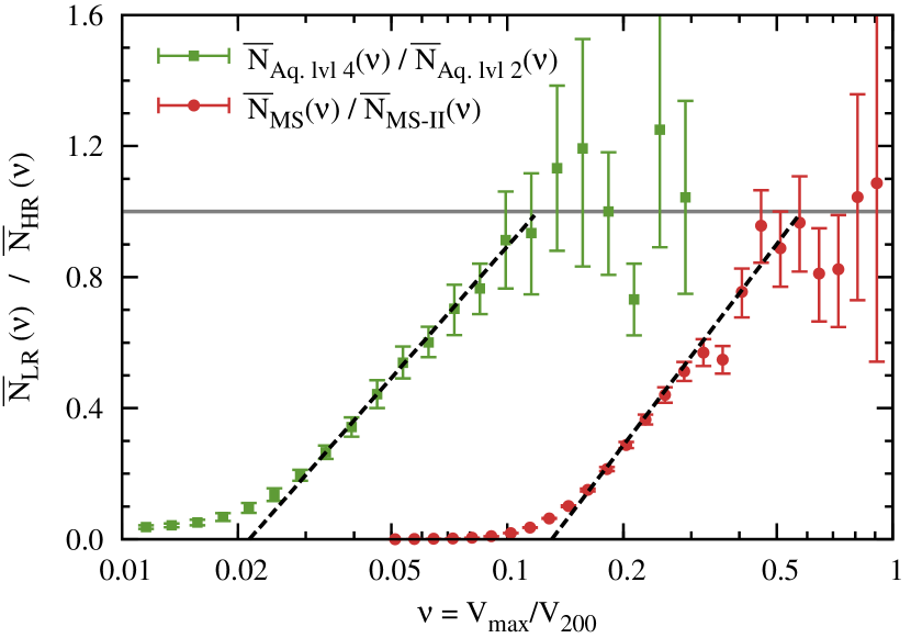
Figure 1: Comparison of the mean subhalo number, $\overline{N}(\nu)$, between equal mass haloes resolved at two different resolutions. The circles show halos in the mass range $(0.6-1.2)\times 10^{13}~{}h^{-1}\rm{M}_{\odot}$ that were resolved with $(0.7-1.4)\times 10^{4}$ particles in the MS and with $125$ times more particles in the MS-II. The squares compare $\overline{N}(\nu)$ of the Aquarius halos resolved with ${\sim}10^{7}$ particles at “level-4” and with ${\sim}20$ times more particles at “level-2”. The dashed curve shows that the transition from $1$ to $0$ is well approximated by a linear function in $\ln\nu$. The error bars represent the $1\sigma$ uncertainty in the determination of the ratio between the two subhalo numbers.

To estimate the completeness function we compare the substructure count between halos in simulations with two different resolutions. The result is illustrated in Fig. 1 where we contrast the mean subhalo count of $(0.6-1.2)\times 10^{13}~{}h^{-1}\rm{M}_{\odot}$ mass halos that were resolved at low resolution in MS and at high resolution in the MS-II. To emphasise the difference we plot the ratio, $\overline{N}_{\mathrm{\textsc{MS}}}(\nu)/\overline{N}_{\mathrm{\textsc{MS-II}}}(\nu)$, between the subhalo count in the two simulations. Since ${\sim}10^{13}~{}h^{-1}\rm{M}_{\odot}$ mass halos in the MS-II have over $10^{6}$ particles, we expect $\overline{N}_{\mathrm{\textsc{MS-II}}}(\nu)$ to be unaffected by numerical effects for $\nu\raisebox{-1.29167pt}{\mbox{$\stackrel{{\scriptstyle>}}{{{}_{\sim}}}\,$}}0.15$ (for a detailed justification of this point see Appendix A.1). This implies that for $\nu\raisebox{-1.29167pt}{\mbox{$\stackrel{{\scriptstyle>}}{{{}_{\sim}}}\,$}}0.15$ we have $\overline{N}_{\mathrm{\textsc{MS-II}}}(\nu)\approx\widetilde{N}(\nu)$ and so, according to Eqn. (5), the ratio $\overline{N}_{\mathrm{\textsc{MS}}}(\nu)/\overline{N}_{\mathrm{\textsc{MS-II}}}(\nu)$ gives the completeness function of MS halos.

Fig. 1 shows that the completeness function is flat and equal to 1 at values of $\nu>0.4$, indicating that in that range the MS recovers the full population of substructures. At lower values of $\nu$, the completeness function decreases from 1 to 0 reflecting the fact that only a partial population of subhalos is found in that range in the MS. This is in agreement with the qualitative expectation discussed above. The transition in the MS completeness function from 1 to 0 is well approximated by a linear function of $\log\nu$, as shown by the dashed line in the figure. Therefore, we can write the completeness function as:

$$f(\nu)=\begin{cases}1&\nu\geq\nu_{0}\vspace{.1cm}\\ 1+\alpha\ln\left(\dfrac{\nu}{\nu_{0}}\right)&\nu_{*}<\nu<\nu_{0}\vspace{.1cm}\\ 0&\nu<\nu_{*},\end{cases}$$ (6)

where $\alpha$ and $\nu_{0}$ are two free parameters (and $\ln$ denotes the natural logarithm). The $\alpha$ parameter gives the slope of the transition from 1 to 0, while $\nu_{0}$ gives the smallest value of $\nu$ for which the simulation identifies all the substructures. The symbol, $\nu_{*}=\nu_{0}e^{-1/\alpha}$, denotes the point below which no more subhalos are detected. This expression gives a very good match to the completeness function as long as $f(\nu)\raisebox{-1.29167pt}{\mbox{$\stackrel{{\scriptstyle>}}{{{}_{\sim}}}\,$}}0.2$, as can be seen in the figure.

In Appendix A.2 we show that the two parameter fit in Eqn. (6) gives a very good description of the completeness function not only for the MS and Aquarius haloes, but also for the MS-II and WMAP7 simulations. Furthermore, we have checked that the same holds true when using different halo finders.

Thus, computing the completeness function of any given simulation reduces to finding the $\nu_{0}$ and $\alpha$ parameters introduced in Eqn. (6). We propose two different methods to calculate these parameters. These procedures are described in detail in Appendix A and can be summarised as follows:

1. Method A is the standard procedure of comparing halos of equal mass in simulations of different resolution. We used this method to compute $f(\nu)$ for the MS by comparing with the higher resolution MS-II data. While this method is simple to implement, it has the drawback that it requires an additional simulation with ${\sim}100$ times higher mass resolution than the simulation of interest. Therefore, we can use method A for MS, but not for the MS-II and WMAP7 since we do not have access to even higher resolution simulations. We introduce method A merely to show that our second technique, method B, gives reliable results.

2. Method B compares the subhalo population in low and high-mass halos in the same simulation. The procedure is based on the assumption that the mean subhalo count is self-similar amongst host halos of different masses (see Wang et al., 2012, and references therein). As we shall see in Section 5, this assumption is satisfied to a good approximation for dark matter substructures but the addition of baryons and feedback processes would break the self-similar behaviour so it is unclear if this procedure can be modified to work in realistic hydrodynamical simulations of galaxy formation. Compared to method A, method B does not require a higher resolution simulation. This represents a great advantage and allows us to compute the completeness function for the MS-II and WMAP7 simulations.

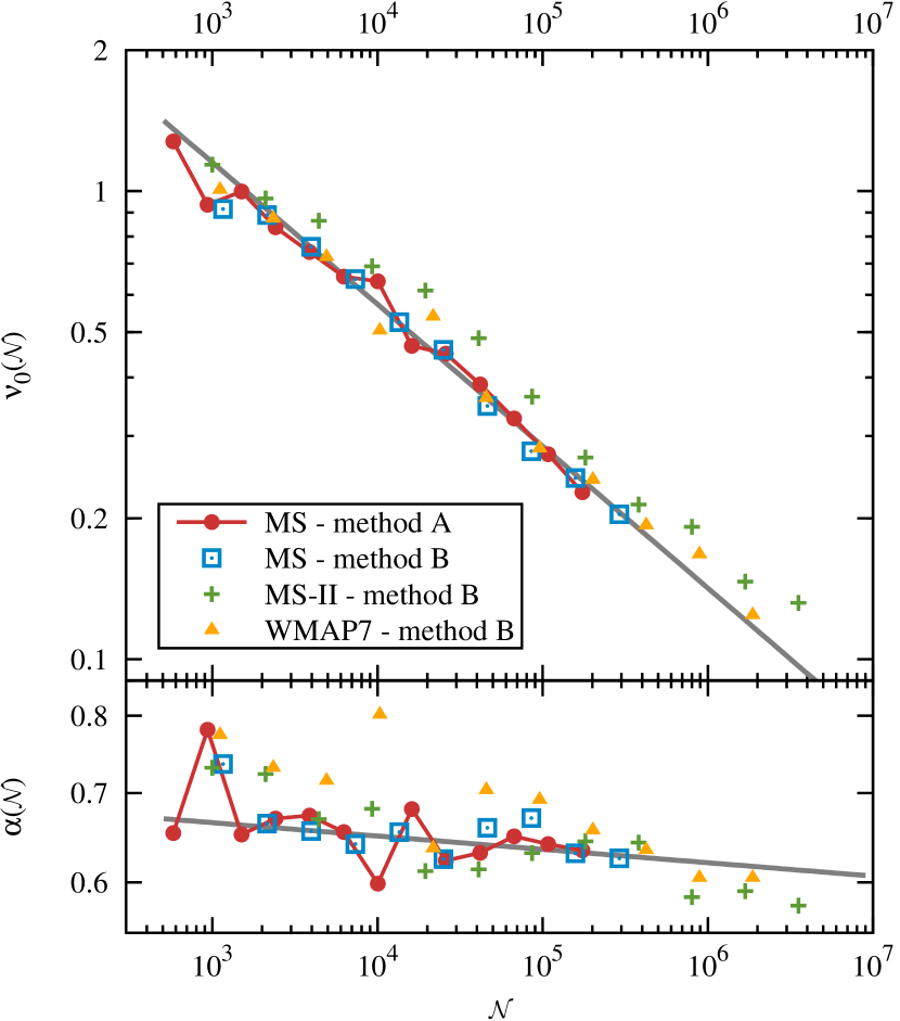
Figure 2: The dependence of the completeness function fit parameters, $\nu_{0}$ (top panel), and $\alpha$ (lower panel), on the number of particles, $\mathcal{N}$, in the host halo. The fit parameters were determined using the two different methods, A and B, described in Appendix A. The solid grey line shows a power-law fit to the results of method A. The power-law fits to each of the simulations are given in Table 2.

Table 2: The values of the variables $\nu_{0}^{0}$, $n_{\nu_{0}}$, $\alpha^{0}$ and $n_{\alpha}$ given in Eqn. (7). These quantities give the dependence of the fitting parameters of the completeness function, $\nu_{0}$ and $\alpha$, on the number of particles, $\mathcal{N}$, in the host halo. We give values for subhalos within distance, $R_{200}$, and, $R_{100}$, from the host halo centre. The $1\sigma$ error in the fit for $\nu_{0}^{0}$ and $\alpha^{0}$ is 0.02, while that for $n_{\nu_{0}}$ and $n_{\alpha}$ is 0.01.

Method - simulation	$\displaystyle\nu_{0}^{0}$	$\displaystyle n_{\nu_{0}}$	$\displaystyle\alpha^{0}$	$\displaystyle n_{\alpha}$
$R_{200}$ substructures
method A - MS	0.57	-0.30	0.65	-0.01
method B - MS	0.57	-0.31	0.65	-0.01
method B - MS-II	0.67	-0.29	0.67	-0.02
method B - WMAP7	0.57	-0.29	0.72	-0.03
$R_{100}$ substructures
method A - MS	0.55	-0.30	0.65	-0.02
method B - MS	0.55	-0.31	0.65	-0.01
method B - MS-II	0.67	-0.29	0.65	-0.03
method B - WMAP7	0.56	-0.28	0.72	-0.04

Using the two methods above we estimate the completeness function for host halos of different mass. We find that the two fitting parameters for $f(\nu)$ in Eqn. (6) depend most strongly on the number of particles, $\mathcal{N}$, used to resolve the host halo. This relationship is illustrated in Fig. 2. The $\alpha$ and $\nu_{0}$ parameters show a power-law dependence on $\mathcal{N}$:

$$\nu_{0}(\mathcal{N})=\nu_{0}^{0}\left(\frac{\mathcal{N}}{10^{4}}\right)^{n_{\nu_{0}}}\mbox{\,\,\, and \,\,\, }\alpha(\mathcal{N})=\alpha^{0}\left(\frac{\mathcal{N}}{10^{4}}\right)^{n_{\alpha}}.$$ (7)

The quantities, $\nu_{0}^{0}$, $n_{\nu_{0}}$, $\alpha^{0}$ and $n_{\alpha}$, are constants that depend on the numerical parameters of the simulation, but not on $\mathcal{N}$. The two expressions in Eqn. (7) give a very good description of $\nu_{0}(\mathcal{N})$ and $\alpha(\mathcal{N})$. This is clearly shown in the figure by the grey line which gives a power-law fit to the results of method A applied to the MS (solid red line with circular symbols). The power law fits to $\alpha$ and $\nu_{0}$ for the three simulations shown in Fig. 2 are given in Table 2. All the simulations show the same qualitative behaviour, though the exact values differ slightly. The quantity $\nu_{0}$ varies as $\mathcal{N}^{-0.3}$, which is close to, but shallower than the $\mathcal{N}^{-1/3}$ dependence that a naive kinematic analysis would suggest. The parameter $\alpha$ varies only slightly, as $\mathcal{N}^{-0.02}$.

Fig. 2 shows that the two methods, A and B, for estimating the completeness function give the same results. This is clearly seen when comparing the values of $\nu_{0}$ and $\alpha$ for the MS simulation obtained using method A (solid red line) and method B (blue square symbols). Thus, $f(\nu)$ can be computed only using the information available in the simulation under study without the use of a higher resolution simulation, by following the method B procedure outlined in Appendix A.2.

In addition, Fig. 2 shows that there are small differences between the completeness function of the three simulations studied here (see also Table 2). Therefore, when precise results are needed, it is necessary to estimate $f(\nu)$ separately for each simulation. Computing the completeness function of a given simulation can be done with minimal computational resources using method B.

The results presented up to now are for substructures within distance, $R_{200}$, of the host halo centre. We find that the fitting formula of Eqn. (6) with very similar parameter values also describes well the completeness function for subhalos within $R_{100}$ of the host halo centre (see Table 2).

3.2 Step II: adding the missing subhalos

As we have seen, the completeness function can be used to estimate the mean abundance of poorly resolved or unresolved subhalos as a function of $V_{\mathrm{max}}$. However, in practice, it is necessary to know not only the mean value of $\overline{N}({>}\nu){}$, but also its dispersion $\sigma({>}\nu){}$ across the halo population, which characterises the halo-to-halo variation.

Given a completeness function, $f(\nu)$, lack of resolution implies that a sample of $n_{\mathrm{hosts}}$ halos are missing a fraction, $1-f(\nu)$, of their substructures. In total, the sample of halos is missing a number of subhalos with velocity ratio, $\nu$, given by,

$$n_{\mathrm{hosts}}\;(1-f(\nu))\;\widetilde{N}(\nu)=n_{\mathrm{hosts}}\;\dfrac{1-f(\nu)}{f(\nu)}\;\overline{N}(\nu){},$$ (8)

where $\widetilde{N}(\nu)$ and $\overline{N}(\nu)$ are the true and measured mean subhalo count (Eqn. (5)). To recover the true substructure count per halo, $\widetilde{N}(\nu)$, we add the missing subhalos to the halo sample by randomly assigning each new subhalo to a host. We take the probability that a new subhalo is assigned to host halo, $i$, to be proportional to $1-f(\nu,\mathcal{N}_{i})$, with $\mathcal{N}_{i}$ the number of particles in host halo $i$. The special case when the sample contains halos of similar mass corresponds to each halo having equal weight, and so we distribute the missing substructures among the hosts with equal probability.

We apply the procedure above to samples of halos within a narrow mass range and repeat the process independently for samples of halos of different mass. This assumes that halo mass is the only factor that determines the subhalo count and ignores the effects of assembly bias. Previous studies have show that the mean subhalo count depends on halo properties other than mass, like concentration and formation redshift (Gao et al., 2004; Zentner et al., 2005; Shaw et al., 2006; Gao et al., 2011), as well as on the large scale environment of the host (Busha et al., 2011b; Cautun et al., 2014). Assembly bias can be taken into account by further restricting the halo samples to hosts with a given concentration or in a given environment. Neglecting assembly bias does not affect the ability of the method to recover the true mean subhalo count, but can result in a smaller value for the scatter in the count. We do not expect this effect to be significant since Gao et al. (2011) found that the dependence of the substructure number count on halo properties is not the main driver of the observed halo-to-halo scatter.

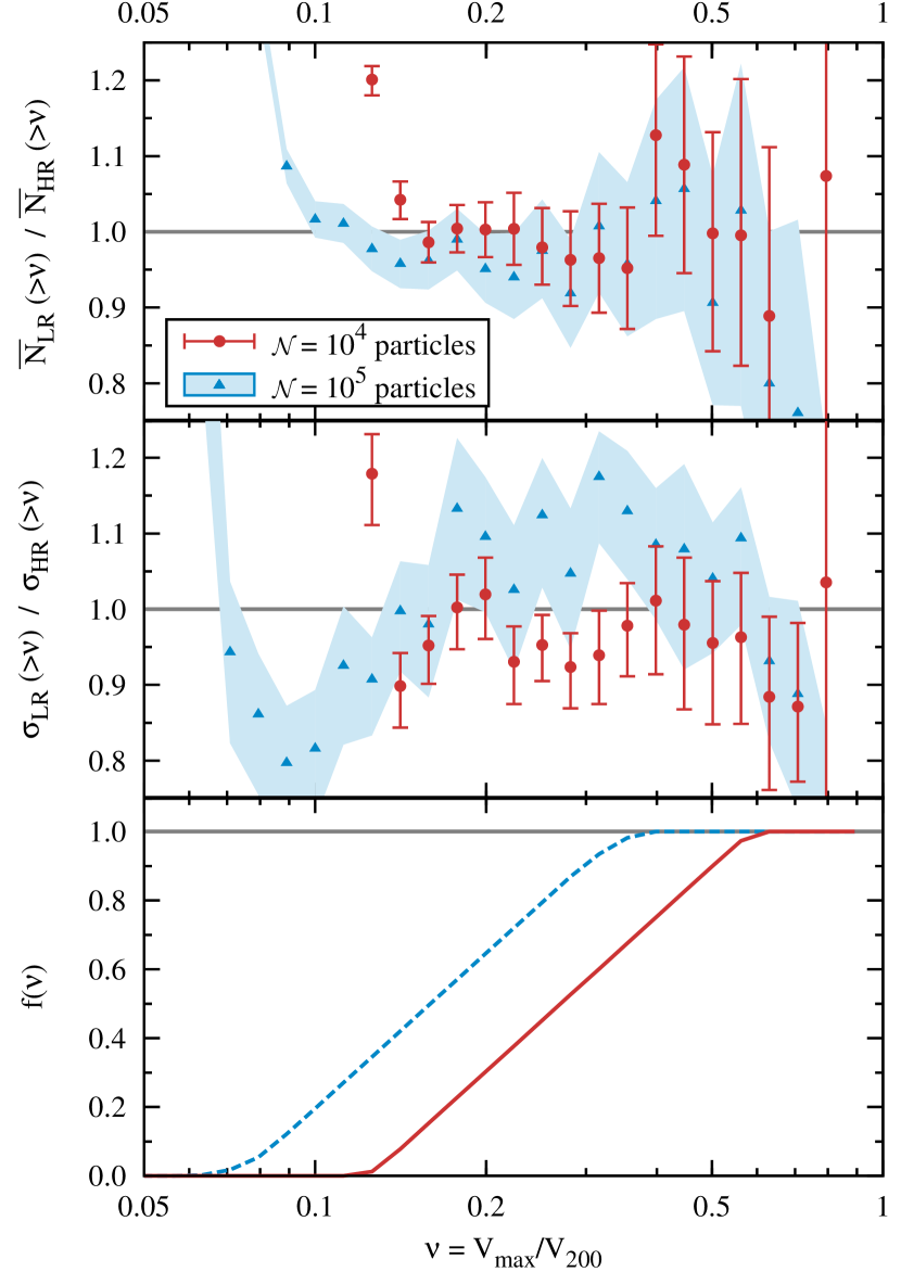
Figure 3: The effectiveness of our extrapolation method for subhalo statistics below the resolution limit of a simulation. The plots compare the mean, $\overline{N}({>}\nu){}$ (top), and scatter, $\sigma({>}\nu){}$ (middle) of the subhalo abundance in low and high resolution simulations. A value of one corresponds to a successful recovery of the mean and scatter. The low resolution data are MS halos resolved with $(0.8-1.2)\times 10^{4}$ (red circles) and $(0.4-1.2)\times 10^{5}$ (blue triangles) particles. The high resolution data are MS-II halos of corresponding mass. The error bars show the $1\sigma$ uncertainty in the determination of $\overline{N}({>}\nu){}$ and $\sigma({>}\nu){}$. The bottom panel shows the completeness function, $f(\nu)$, corresponding to the low resolution halo samples: red for $\mathcal{N}{\sim}10^{4}$ and dashed blue for $\mathcal{N}{\sim}10^{5}$. The extrapolation procedure is applied only in the region $f(\nu){<}1$; for $f(\nu){=}1$ there are no additional subhalos added.

3.3 Evaluation of the extrapolation procedure

Fig. 3 shows how successful the extrapolation method is in recovering the mean, $\overline{N}({>}\nu){}$, and standard deviation, $\sigma({>}\nu){}$, of the subhalo population. The top panel gives the ratio, $\overline{N}_{\mathrm{LR}}({>}\nu)/\overline{N}_{\mathrm{HR}}({>}\nu)$, between the mean subhalo count found at low and high resolution as a function of the velocity ratio, $\nu$. The middle panel gives the ratio, $\sigma_{\mathrm{LR}}({>}\nu)/\sigma_{\mathrm{HR}}({>}\nu)$, between the scatter in the subhalo counts found at low and high resolution. In both cases a value of one corresponds to a successful recovery of the true mean and scatter in the number of subhalos. We illustrate the result of the extrapolation method for host halos resolved with ${\sim}10^{4}$ (red circles) and ${\sim}10^{5}$ (blue triangles) particles in the MS simulation. The two datasets show the comparison for halos in the mass range $(0.69-1.1)\times 10^{13}~{}h^{-1}\rm{M}_{\odot}$ and $(0.35-1.2)\times 10^{14}~{}h^{-1}\rm{M}_{\odot}$ respectively, which were resolved at relatively low resolution in the MS and at higher resolution in the MS-II.

The bottom panel of Fig. 3 shows the completeness function, $f(\nu)$, of MS halos resolved with ${\sim}10^{4}$ and ${\sim}10^{5}$ particles. For $f(\nu)=1$ there is no correction since the number of new subhalos that need to be added is proportional to $(1-f(\nu))/f(\nu)$ (see Eqn. (8)). The correction becomes important only when $f(\nu)$ is significantly smaller than unity. The top panel of the figure shows that we obtain $\overline{N}_{\mathrm{LR}}({>}\nu)/\overline{N}_{\mathrm{HR}}({>}\nu)\approx 1$ down to values of $\nu$ equal to 0.14 and 0.09 for halos resolved with ${\sim}10^{4}$ and ${\sim}10^{5}$ particles respectively. These values of $\nu$ correspond to the range where $f(\nu)\raisebox{-1.29167pt}{\mbox{$\stackrel{{\scriptstyle>}}{{{}_{\sim}}}\,$}}0.15$ as may be seen by comparing to the bottom panel of the figure. Thus, our extrapolation method is successful at recovering the true mean subhalo number count as long as $f(\nu)\raisebox{-1.29167pt}{\mbox{$\stackrel{{\scriptstyle>}}{{{}_{\sim}}}\,$}}0.15$.

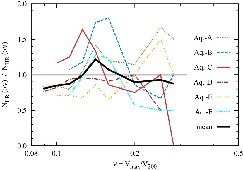
Figure 4: An object-to-object comparison of the subhalo count for the six Aquarius haloes, $N_{\mathrm{HR}}({>}\nu)$, and the corrected subhalo count of their MS-II counterparts, $N_{\mathrm{LR}}({>}\nu)$. The solid black line compares the mean substructure number in the two samples. The results reiterate that the extrapolation method gives the correct subhalo statistics although the scatter is appreciable for individual objects.

For the scatter in the subhalo number count, we find from the centre panel of Fig. 3 that $\sigma_{\mathrm{LR}}({>}\nu)/\sigma_{\mathrm{HR}}({>}\nu){\approx}1$ down to values of $\nu$ of 0.16 and 0.11 for halos resolved with ${\sim}10^{4}$ and ${\sim}10^{5}$ particles respectively. Therefore, our extrapolation technique recovers the correct subhalo scatter in the region where $f(\nu)\raisebox{-1.29167pt}{\mbox{$\stackrel{{\scriptstyle>}}{{{}_{\sim}}}\,$}}0.3$. In the case of the second dataset, we observe variations from unity of order $10\%$. These are due to the small sample of only $70$ MS-II halos found in that mass range, which does not allow for a precise enough estimate of the scatter in the subhalo number count using bootstrap techniques. More importantly, we do not find any obvious systematic effects in the estimate of $\sigma({>}\nu){}$, except, at most, a $5\%$ lower than expected value for $f(\nu)\raisebox{-1.29167pt}{\mbox{$\stackrel{{\scriptstyle<}}{{{}_{\sim}}}\,$}}0.5$. This implies that we can neglect subhalo assembly bias and still recover, to a good approximation, the true subhalo scatter. We also checked the effectiveness of the extrapolation procedure for the MS-II and WMAP7 simulations and found similar behaviour to the MS case presented here.

As a further test, we can compare the galactic mass halos in the Aquarius simulations with their counterparts in the MS-II that have ${\sim}1000$ times fewer particles. With only six examples, it is not possible to carry out a statistical comparison but since the Aquarius halos are resimulations of MS-II halos we can perform an object-to-object comparison. This is shown in Fig. 4. We find that the ratio, $N_{\mathrm{LR}}({>}\nu)/N_{\mathrm{HR}}({>}\nu)$, between the low and high resolution results oscillates around one, without any obvious systematic trend. This shows that the extrapolation method faithfully recovers the statistics of the population over a large dynamical range in $\nu$.

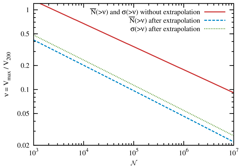
Figure 5: The lowest value of $\nu$ for which we recover the mean, $\overline{N}({>}\nu){}$, and the dispersion, $\sigma({>}\nu){}$, of the subhalo abundance. These limits are a function of the number of particles, $\mathcal{N}$, in the host halo. The solid curve gives the lower limits in the absence of extrapolation. The dashed and dotted curves give the of values of $\overline{N}({>}\nu){}$ and $\sigma({>}\nu){}$ respectively when extrapolating below the resolution limit. While the results shown here are for MS-II, the other two simulations show a very similar behaviour, as may be seen in Fig. 2.

In Fig. 5 we show the values of $\nu$ above which we recover the true subhalo population with our extrapolation method. The solid curve gives the $\nu$ limit in the absence of extrapolation, given by the value of $\nu_{0}$ for MS-II from Table 2. The dashed and dotted curves give the $\nu$ limits for the mean and dispersion in the subhalo number count when applying our extrapolation method. They were obtained by solving the $f(\nu)=0.2$ and $f(\nu)=0.3$ equations and correspond to conservative lower limits for recovering $\overline{N}({>}\nu){}$ and $\sigma({>}\nu){}$ as found in Fig. 3. By using our scaling method we can estimate $\overline{N}({>}\nu){}$ and $\sigma({>}\nu){}$ to much lower $\nu$ values, corresponding to simulations with at least 50 times higher mass resolution.

4 The abundance of subhalos in MW-mass halos

4.1 Mean subhalo number

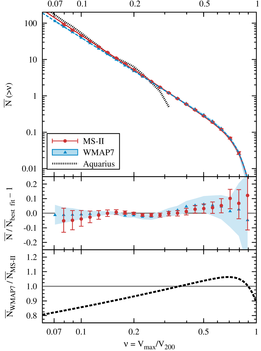
Figure 6: Top: the corrected mean subhalo count as a function of the velocity ratio, $\nu$, in MW-mass halos in the MS-II and WMAP7 simulations. The two lines show the best fit function given by Eqn. (9) for MS-II (solid red) and WMAP7 (dashed blue). The dotted curve shows $\overline{N}({>}\nu){}$ for the six Aquarius halos. Middle: the ratio between the actual number of subhalos in the simulations and the number given by the best fit function to the data in the top panel. The errors bars give the $1\sigma$ error in the estimate of $\overline{N}({>}\nu){}$ due to finite sample effects (which dominate for $\nu{>}0.3$) and due to uncertainties in the estimate of the completeness function (which dominate for $\nu{<}0.2$). Bottom: ratio of the best fit function to the subhalo abundance in the MS-II and WMAP7 simulations.

In this section we investigate the subhalo distribution within halos in the mass range $(0.6-2.2)\times 10^{12}~{}h^{-1}\rm{M}_{\odot}$ to which we refer as MW-like or MW-mass host halos. This mass range is consistent with estimates of the MW halo mass obtained through a variety of methods (Wilkinson & Evans, 1999; Sakamoto, Chiba & Beers, 2003; Battaglia et al., 2005; Dehnen, McLaughlin & Sachania, 2006; Smith et al., 2007; Li & White, 2008; Xue et al., 2008; Gnedin et al., 2010; Guo et al., 2010; Watkins, Evans & An, 2010; Busha et al., 2011a; Piffl et al., 2014).

Using the extrapolation technique described in the previous section we can recover the mean subhalo number, $\overline{N}({>}\nu){}$, for $\nu\geq 0.08$ (compared to $\nu\geq 0.3$ in MS-II and WMAP7 in the absence of these corrections). We illustrate this in Fig. 6 where we show the corrected $\overline{N}({>}\nu){}$ for MW-like hosts in the MS-II and WMAP7 simulations. The mean subhalo velocity function has a power law dependence at small $\nu$ and an exponential cut-off at large $\nu$. As BK10 did, we find that the function:

$$N({>}\nu){}=\left(\frac{\nu}{\nu_{1}}\right)^{a}\exp\left(-\left(\frac{\nu}{\nu_{\mathrm{cut}}}\right)^{b}\right)$$ (9)

gives a good match to the cumulative mean number of substructures as a function of $\nu$ for MW mass halos. Following the prescription given by BK10 we fit the mean subhalo abundance for both MS-II and WMAP7. The resulting best fit parameters for the two simulations are given in Table 3. The best fit function fits the data very well, as may be seen in the middle panel of Fig. 6.

Table 3: The best fit parameters of Eqn. (9) for the mean subhalo number count in MW-like halos in the MS-II and WMAP7 simulations, within both $R_{200}$ and $R_{100}$ from the host halo centre. The $1\sigma$ errors in the fit are at most, $\Delta a=0.02$, $\Delta\nu_{1}=0.003$, $\Delta b=1$ and $\Delta\nu_{\mathrm{cut}}=0.02$. The value of the parameter $a$ is sensitive to errors in the estimate of the completeness function (see Table 2), which introduces an additional systematic error of $\Delta a=0.07$.

Simulation	Subhalos within	$a$	$\nu_{1}$	$b$	$\nu_{\mathrm{cut}}$
MS-II	$R_{200}$	-3.17	0.338	7	0.80
WMAP7		-3.05	0.336	7	0.79
MS-II	$R_{100}$	-3.22	0.366	7	0.80
WMAP7		-3.12	0.364	7	0.79

The MS-II and WMAP7 halos have the same number of massive substructures, but there are important differences between the two simulations for low values of $\nu$. The subhalo population in MS-II halos has a slightly steeper slope and thus a higher abundance at low $\nu$ than in WMAP7 halos. From the bottom panel of Fig. 6, it can be seen that for WMAP-7 cosmological parameters, MW-like halos have only $93\%$ and $86\%$ of the MS-II subhalos at $\nu=0.2$ and $\nu=0.1$ respectively.

When comparing with results in the literature, we find that other studies have systematically underestimated the substructure abundance at low $\nu$ as a result of not taking finite resolution effects properly into account. Thus, while BK10 found similar values for the $\nu_{\mathrm{cut}}$ and $b$ fit parameters for MS-II subhalos, they underestimated the slope of the velocity function at low $\nu$: they find $a=-2.98$ whereas for substructures within $R_{100}$ we find $a=-(3.22\pm 0.09)$. The discrepancy in slope is due to BK10 fitting the subhalo count down to $\nu=0.2$, while we find that without proper correction, the MS-II simulation gives the correct subhalo abundance only for $\nu\geq 0.3$. In contrast, Wang12 found a slope of $a=-3.11$ within $R_{200}$, which agrees within the errors with our value of $a=-(3.17\pm 0.09)$, but nevertheless they find $20\%$ fewer subhalos within $R_{200}$ at all values of $\nu$.

The main difference between Wang12 and BK10 is that, just as we have done, Wang12 used the invariance of $\overline{N}({>}\nu){}$ with host halo mass to estimate the average subhalo abundance. This approach appears to give the correct value for the slope, $a$. However, as BK10 did, Wang12 overestimated the value of $\nu$ at which resolution effects become important and their fits to $\overline{N}({>}\nu){}$ included host halos for which only ${\sim}75\%$ of substructures are detected. Another difference with these studies is that we use a phase-space halo finder while both BK10 and Wang12 use a configuration-space halo finder. However, we expect that this choice accounts for at most a few percent of the difference, as we show in Appendix B.

4.2 Scatter in the substructure population

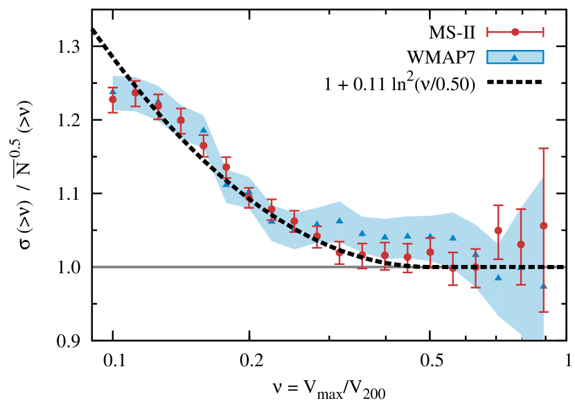
Figure 7: The dependence of the scatter in the subhalo abundance, $\sigma({>}\nu){}$, on the velocity ratio, $\nu$, for MW-like hosts. For clarity we show $\sigma({>}\nu){}/\overline{N}^{1/2}({>}\nu){}$, the ratio between the observed scatter and the Poisson value, $\overline{N}^{1/2}({>}\nu){}$. The dashed black curve gives the fit to the data for both the MS-II and WMAP7 simulations, with the best-fit parameters quoted in the legend. The error bars represent the $1\sigma$ error in $\sigma({>}\nu){}$.

The dispersion of the subhalo number distribution characterises halo-to-halo variations and is important not only for quantifying how typical the MW and its satellites are, but also for the interpretation of conclusions derived from very high-resolution simulations of a few MW-sized halos (Diemand et al., 2008; Springel et al., 2008; Stadel et al., 2009). The scatter in the subhalo abundance is also an important parameter when applying halo occupation distribution (HOD) models to populate dark matter halos with galaxies (eg. Benson et al., 2000; Seljak, 2000; Ma & Fry, 2000; Peacock & Smith, 2000; Scoccimarro et al., 2001; Berlind & Weinberg, 2002).

We find that, at large $\nu$, the scatter in the substructure abundance matches the dispersion of a Poisson distribution with the same mean. At lower velocity ratios, as the average number of subhalos increases, we find a much larger scatter than expected for a Poisson distribution. This is illustrated in Fig. 7 that shows the ratio of the measured subhalo scatter to the dispersion, $\overline{N}^{1/2}({>}\nu){}$, of a Poisson distribution with mean $\overline{N}({>}\nu){}$. We find that the standard deviation, $\sigma({>}\nu){}$, in both the MS-II and WMAP7 subhalo distributions has the same dependence on $\nu$ that can be parametrised as:

$$\sigma({>}\nu)=\overline{N}^{1/2}({>}\nu)\begin{cases}1&\nu\geq\nu_{\sigma}\\ 1+\beta\ln^{2}(\nu/\nu_{\sigma})&\nu<\nu_{\sigma}.\end{cases}$$ (10)

Fitting this equation to the data, we find $\nu_{\sigma}=0.50$ and $\beta=0.11$. This fit is a very good match to the subhalo abundance scatter, as may be seen in Fig. 7. The scatter for substructures within $R_{100}$ from the host halo centre shows a similar functional form, but with best-fit parameters $\nu_{\sigma}=0.55$ and $\beta=0.14$.

Our result that the scatter in the number of small substructures differs significantly from the Poissonian expectation is in good agreement with previous results: Benson et al. (2000) showed that the occupation of halos by galaxies is not a Poisson process and BK10 showed that the dispersion in the number of subhalos above a certain mass is a combination of Poisson scatter at the high mass end and larger than Poisson scatter at the low mass end.

4.3 Subhalo occupation distribution

Figure 8: The probability distribution function of the number of substructures in MW-like host halos with $\nu\geq 0.3$ (top), $\nu\geq 0.2$ (middle) and $\nu\geq 0.1$ (bottom). The solid and dashed curves show the negative binomial distribution with the mean and standard deviation found in Figures 6 and 7. The solid grey curve in the bottom panel shows a Poisson distribution with the same mean as the MS-II halos.

Since the scatter in the subhalo population is significantly non-Poissonian, we follow BK10 and Busha et al. (2011b), and model the probability distribution function (PDF) of the number of substructures with a given value of $\nu$ using the negative binomial distribution (NBD),

$$P(N|r,s)=\frac{\Gamma(N+r)}{\Gamma(r)\Gamma(N+1)}s^{r}(1-s)^{N},$$ (11)

where $N$ is the number of subhalos per halo, $\Gamma(x)=(x-1)!$ is the Gamma function, which, for integer values of $x$, reduces to the factorial function, and $r$ and $s$ are two parameters. The mean and dispersion of this distribution can be computed analytically in terms of $r$ and $s$. The inverse holds too, with the two distribution parameters given by:

$$r=\frac{\mu^{2}}{\sigma^{2}-\mu}\mbox{ ,\hskip 28.45274pt }s=\frac{\mu}{\sigma^{2}},$$ (12)

where $\mu$ and $\sigma$ denote the mean and dispersion of the NBD. Thus, $\mu$ and $\sigma$ completely specify the distribution. The NBD has also been used to describe the number of satellite galaxies in HOD models (eg. Berlind & Weinberg, 2002).

BK10 found that the NBD gives a better fit to the substructure population than a Poisson distribution when counting all subhalos containing more than a certain fraction of the host mass. We find that the NBD also matches well the substructure PDF when counting all subhalos with velocity ratios larger than $\nu$. This is illustrated in Fig. 8 where we plot the subhalo occupation distribution for MW-mass hosts in both the MS-II and WMAP7 simulations. The solid and dashed lines NBDs. These are not fits to the data points, but are obtained from Eqn. (12) using the mean subhalo number, $\overline{N}({>}\nu){}$, from Eqn. (9) and the dispersion, $\sigma({>}\nu){}$, from Eqn. (10). It is clear in the figure that the NBD reproduces very well the subhalo distribution at all values of $\nu$. Therefore, knowing the mean and scatter of the subhalo number counts is enough to infer the full PDF.

The grey line in the lower panel of Fig. 8 shows a Poisson distribution with the same mean as the MS-II subhalo abundance. It is clear that the Poisson distribution severely underestimates the tails of the PDF. Thus, even a modest increase in the dispersion compared to the Poisson case ($25\%$ at $\nu=0.1$) leads to large deviations from a Poisson distribution.

5 Dependence of subhalo number on host mass

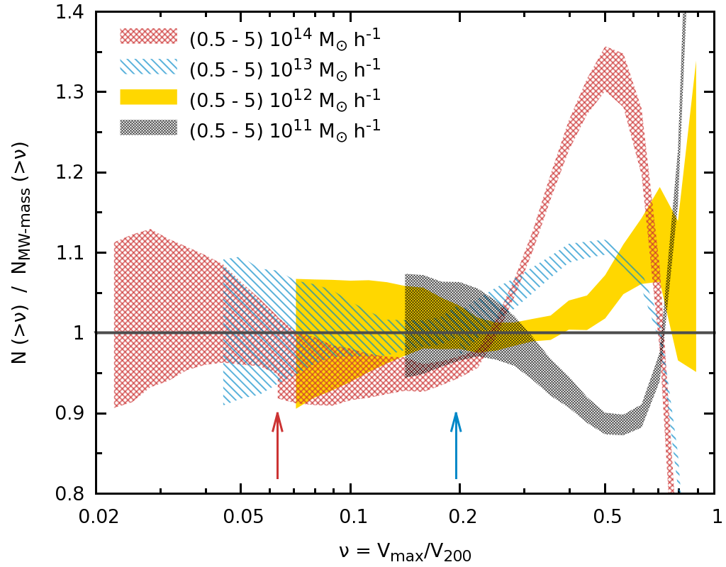
Figure 9: The dependence of the abundance of substructures as a function of $\nu$, $N({>}\nu){}$, on the host halo mass. To emphasise the differences, we divide by the mean subhalo number, $\overline{N}_{\mathrm{MW-mass}}({>}\nu){}$, for MS-II MW-like hosts. The two vertical arrows indicate the $\nu$ value where we switch from MS to MS-II data for hosts of mass $(0.5-5)\times 10^{14}~{}h^{-1}\rm{M}_{\odot}$ (red arrow) and $(0.5-5)\times 10^{13}~{}h^{-1}\rm{M}_{\odot}$ (blue arrow). The other two mass bins show only MS-II halos. The width of each curve shows the $1\sigma$ error in the determination of $N({>}\nu){}$.

In Fig. 9 we investigate how the mean number of substructures as a function of normalized velocity, $\nu$, varies for hosts of different mass. To emphasise the differences, we normalise the mean subhalo number count in each mass bin by the mean, $\overline{N}_{\mathrm{MW-mass}}({>}\nu){}$, for MW-mass hosts. We find that for $\nu\leq 0.3$ there is very little dependence on host halo mass, with at most a $5\%$ difference between MW-like and cluster sized halos. In contrast, for larger subhalos we find a complex variation with host mass that can be split in the two regimes. Substructures with $\nu\raisebox{-1.29167pt}{\mbox{$\stackrel{{\scriptstyle>}}{{{}_{\sim}}}\,$}}0.8$ tend to be much more common in lower mass halos than in high mass ones. Thus, it is much more likely to find a halo-subhalo pair of similar mass in MW-like and lower mass hosts than in cluster sized objects. In the $0.3\raisebox{-1.29167pt}{\mbox{$\stackrel{{\scriptstyle<}}{{{}_{\sim}}}\,$}}\nu\raisebox{-1.29167pt}{\mbox{$\stackrel{{\scriptstyle<}}{{{}_{\sim}}}\,$}}0.7$ range this trend is reversed, with more subhalos present in massive hosts than in less massive ones. In this case, the increase of $\overline{N}({>}\nu){}$ with the mass of the host is small, with ${\sim}15\%$ variation in the number of substructures per decade of host halo mass.

The results in Fig. 9 support the assumption we made in Section 3 that the mean subhalo count as a function of $\nu$ varies only slowly or not at all with host halo mass. This explains why method B works is valid for estimating the completeness function. This also means that our results for the subhalo population of MW-like halos are insensitive to the exact mass range used to define MW-mass halos. The invariance of the mean substructure count on host mass makes it possible to use host halos of all masses to compute $\overline{N}({>}\nu){}$, but only for $\nu\leq 0.3$. This property was already exploited by Wang12, who used halos in a large mass range to investigate the subhalo population of MW-like halos and derive constraints on the MW halo mass.

The number of subhalos is independent of host halo mass only when expressed in terms of the ratio $\nu=V_{\mathrm{max}}^{\mathrm{subhalo}}/V_{\mathrm{200}}^{\mathrm{host}}$. Previous studies have shown that there is a variation with host halo mass when considering $\overline{N}({>}M^{\mathrm{subhalo}}/M^{\mathrm{host}})$ (Gao et al., 2004; Zentner et al., 2005; Gao et al., 2011) or $\overline{N}({>}V_{\mathrm{max}}^{\mathrm{subhalo}}/V_{\mathrm{max}}^{\mathrm{host}})$ (Klypin, Trujillo-Gomez & Primack, 2011; Busha et al., 2011b).

6 The MW massive satellites

As we discussed in Section 1, the conclusion that the MW has at most three satellites residing in substructures with $V_{\mathrm{max}}\geq 30~{}\rm{km/s}$ – the two Magellanic Clouds and the Sagittarius dwarf – seems at odds with the number of such substructures, eight on average, found in the Aquarius simulations of halos of mass $M_{200}\sim 2\times 10^{12}~{}h^{-1}\rm{M}_{\odot}$ (Boylan-Kolchin, Bullock & Kaplinghat, 2011). The probability of finding such a population of substructures within $\Lambda$CDM was investigated by Wang12 who found that this “too-big-to-fail-problem” is only present if the MW halo has a mass similar to the Aquarius halos, but the problem is avoided altogether if the halo mass is a factor of 2 smaller. They were therefore able to set an upper limit to the MW halo mass under the assumption that $\Lambda$CDM is the correct model. Since we find a higher number of substructures than Wang12 did, we now re-examine how their constraints on the MW mass change when using the subhalo statistics derived in Section 4.

Given a halo of virial velocity, $V_{200}$, the probability that it hosts at most $X$ substructures with $V_{\mathrm{max}}\geq V_{0}$ is given by

$$p({\leq}X,V_{0})=\sum_{k=0}^{X}P(k|r({>}\nu){},s({>}\nu){})\mbox{\hskip 5.69046pt with}\;\nu=\frac{V_{0}}{V_{200}}\,,$$ (13)

where $P(k|r({>}\nu){},s({>}\nu){})$ is the negative binomial distribution that gives the probability that a halo has $k$ subhalos with velocity ratio larger than $\nu$ (see Eq. 11). The distribution parameters, $r({>}\nu){}$ and $s({>}\nu){}$, are uniquely determined by the mean and scatter of the subhalo population through Eqn. (12).

The probability, $p(\leq 3,30~{}\rm{km/s})$, is shown in Fig. 10 as a function of halo virial velocity (lower tick marks) or, equivalently, halo mass (upper tick marks). The results shown are for subhalos identified within $R_{100}$, which is close to the maximum distance at which dwarf galaxies are identified as being MW satellites. The solid blue curve shows $p(\leq 3,30~{}\rm{km/s})$ from the MS-II simulation. The probability is a steep function of host halo mass, decreasing from ${\sim}70\%$ at $0.5\times 10^{12}\rm{M}_{\odot}$ to ${\sim}15\%$ at $1\times 10^{12}\rm{M}_{\odot}$, and becomes negligible for halos more massive than $2\times 10^{12}\rm{M}_{\odot}$. For convenience, we give values of $p(\leq 3,30~{}\rm{km/s})$ in Table 4 for some suggestive halo masses. Therefore, assuming that the $\Lambda$CDM cosmology is the correct model, given that the MW has only three satellites with $V_{\mathrm{max}}\geq 30~{}\rm{km/s}$ it is unlikely that our galaxy’s halo is more massive than ${\sim}1.5\times 10^{12}\rm{M}_{\odot}$.

The dashed orange curve in Fig. 10 shows results for a $\Lambda$CDM model with WMAP-7 parameters. Since this model has fewer substructures at low $\nu$ than a model with WMAP-1 parameters, then, at fixed halo mass, it has a higher $p(\leq 3,30~{}\rm{km/s})$ resulting in a weaker upper limit on the MW halo mass. Nevertheless, because of the steep decline of the probability with halo mass, the upper limit on the MW halo mass is only slightly increased in this model compared to the one with WMAP-1 parameters.

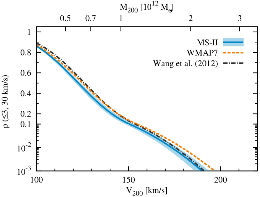
Figure 10: The probability, $p(\leq 3,30~{}\rm{km/s})$, that a halo has at most three substructures with $V_{\mathrm{max}}\geq 30~{}\rm{km/s}$ within a distance $R_{100}$ from its centre. The probability is given as a function of halo virial velocity, $V_{200}$ (lower tick marks), and halo mass, $M_{200}$ (upper tick marks). We show results for both the WMAP-1 cosmology used in MS-II (solid line) as well as for the more recent WMAP-7 parameters (dashed line). The dashed-dotted line shows the results of Wang12. The width of the MS-II curve gives the $1\sigma$ error due to uncertainties in the subhalo abundance of galactic halos. The WMAP7 results have the same error associated with them (not shown). Note that the y-axis is linear above 0.1 and logarithmic for lower values.

Table 4: The probability, $p({\leq}3,30~{}\rm{km/s})$, of finding three or fewer substructures with $V_{\mathrm{max}}\geq 30~{}\rm{km/s}$ for suggestive halo masses. Predictions are given for two choices of cosmological parameters derived from the WMAP-1 and WMAP-7 data, and they are compared to the previous results by Wang12 that are based on WMAP-1 parameters.

Halo mass	$[\times 10^{12}\rm{M}_{\odot}]$	$0.5$	$0.7$	$1$	$2$
WMAP-1	$[\%]$	67	38	13	0.2
WMAP-7	$[\%]$	72	44	20	0.6
Wang12	$[\%]$	76	48	22	0.3

We expect that our results are robust to changes in cosmological parameters, especially concerning the recent Planck Collaboration (2013) measurement. The subhalo abundance could potentially be affected by the change in the concentration of halos and subhalos, but Dutton & Macciò (2014) showed that the increase in $\Omega_{m}$ between the WMAP-1 and Planck measurements is balanced by the decrease in the values of $\sigma_{8}$, $n_{s}$ and $h$, such that halos of the same mass have the same concentration in both cosmologies. In addition, increasing $\Omega_{m}$ leads to a larger number of halos at fixed mass and potentially to more subhalos, but, despite all this, the scaled subhalo velocity function is insensitive to variations in $\Omega_{m}$ (Garrison-Kimmel et al., 2014).

Compared to the previous results of Wang12, we find stricter upper limits for the mass of the MW halo. This is seen in Fig. 10 by comparing the solid and dashed-dotted curves, with both corresponding to WMAP-1 parameters. The main cause of the discrepancy is that Wang12 found up to $20\%$ fewer substructures than we find (see 4.1) and thus overestimated the probability at fixed halo mass. A second source of disagreement is the PDF used to model the subhalo population. Wang12 used a Poisson distribution that underestimates the true tails of the subhalo number distribution (see Fig. 8 for an example). This effect becomes important when dealing with low $p(\leq 3,30~{}\rm{km/s})$ values and leads to an underestimate of the true probability. This is the reason why the Wang12 probability for $M_{200}\raisebox{-1.29167pt}{\mbox{$\stackrel{{\scriptstyle>}}{{{}_{\sim}}}\,$}}10^{12}\rm{M}_{\odot}$ is lower than our value for WMAP-7 parameters, even though we find a larger subhalo count in the latter case.

7 How typical are the Aquarius halos?

In view of the prominence that the Aquarius halo simulations have had, particularly in the work of Springel et al. (2008) and Boylan-Kolchin, Bullock & Kaplinghat (2011, 2012), it is interesting to ask how typical these halos are of the global population of halos of similar mass. BK10 addressed this question in some detail using the MS-II and found that the six Aquarius halos are representative in so far as the properties that they considered (such as assembly history and internal structure) is concerned. However, they did not consider the distribution of $\nu$ that is of most interest here.

In Fig. 11 we compare the cumulative $\nu$ distribution, $N({>}\nu){}$, of each of the six level-2 Aquarius halos with that of the population of MS-II halos in the mass range $(0.6-2.2)\times 10^{12}~{}h^{-1}\rm{M}_{\odot}$. To show the differences more clearly, we normalize the distributions to the the mean, $\overline{N}_{\mathrm{MW-mass}}({>}\nu){}$, of the MS-II. The thick dashed line shows the median for the MS-II population, which is always smaller than the mean count due to the long tail in the subhalo number PDF (see Fig. 8). The light and dark shaded regions show the $68\%$ and $90\%$ scatter around the median obtained by modelling the subhalo distribution function as a NBD with the mean and dispersion values given in Section 4.

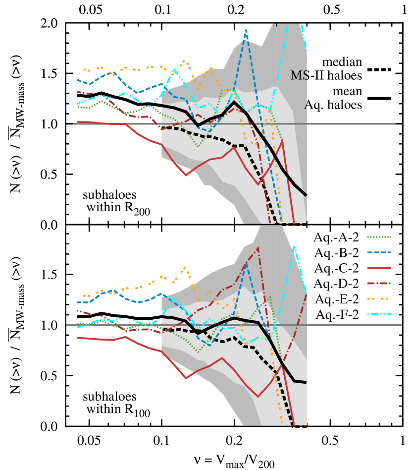
Figure 11: The cumulative distribution, $N({>}\nu){}$, of normalized velocities in each of the six level-2 Aquarius halos compared with that of the global population of halos in the mass range $(0.6-2.2)\times 10^{12}~{}h^{-1}\rm{M}_{\odot}$ in the MS-II. The Aquarius data are normalized to the mean, $\overline{N}_{\mathrm{MW-mass}}({>}\nu){}$, in the MS-II. The top and bottom panels show results for substructures within distance $R_{200}$ and $R_{100}$ from the host halo centre respectively. The thick dashed curve shows the median of the MS-II population while the light shaded region delimits the $16$ and $84$ percentiles of the distribution and the dark shaded region the $5$ and $95$ percentiles. We restrict our analysis to $\nu\leq 0.4$, since only Aq.-F has subhalos with higher $\nu$.

Our comparison of the Aquarius and MS-II subpopulations is restricted to $\nu\geq 0.1$, the resolution limit for MS-II subhalos. For completeness, we present the substructure function of the Aquarius halos down to their resolution limit, $\nu\geq 0.04$, but we do not use the additional range in the comparison with the MS-II.

Fig. 11 shows that the six Aquarius halos have a subhalo normalized velocity function that is in good agreement with the much larger sample of MS-II halos of similar mass, both when considering subhalos within $R_{200}$ (top panel) and within $R_{100}$ (bottom panel). The mean of the Aquarius velocity function lies well within the $68\%$ scatter and it is in very good agreement with the mean in the MS-II. Individually, we find that Aq.-C has the smallest number of subhalos compared to the other Aquarius halos, especially for $\nu\leq 0.25$, but it is still within the MS-II distribution. The remaining five Aquarius halos have a substructure velocity function similar or larger than the median for the MS-II halos. This result agrees with Wang12 who found that five of the Aquarius halos have more substructures with $V_{\mathrm{max}}\geq 30~{}\rm{km/s}$ than the mean.

To summarize, for $\nu\raisebox{-1.29167pt}{\mbox{$\stackrel{{\scriptstyle<}}{{{}_{\sim}}}\,$}}0.25$, five out of the six Aquarius halos have a subhalo normalized velocity function that is similar or larger than the median for a representative sample of MW-mass halos. This needs to be born in mind when comparing the small number of massive satellites present in the MW with the Aquarius halos, especially if, as seems to be the case according to determinations of the satellite luminosity function in the SDSS (Guo et al., 2012; Wang & White, 2012), our galaxy has significantly fewer satellites than average.

8 Summary

We have introduced an extrapolation method to infer subhalo number statistics below the resolution limit of a cosmological simulation. This method statistically generates the correct subhalo abundance from the partial information available in a simulation of limited resolution. We have tested this technique by comparing results of simulations of different resolution - including the high resolution Aquarius simulations - and conclude that it extends the subhalo number counts correctly down to what would be found in a simulation of $50$ times or more better mass resolution. The technique reproduces only the statistics of the subhalo population, not the position or structure of subhalos. We characterized the subhalo abundance in terms of the scaled subhalo velocity function, $\overline{N}({>}\nu){}$, which gives the number of substructures above $\nu=V_{\mathrm{max}}/V_{200}$, where $V_{\mathrm{max}}$ is the subhalo maximum circular velocity and $V_{200}$ the virial velocity of the host. We give a fitting formula for the completeness function as a function of $\nu$ that can be used to extrapolate the results of a simulation.

As noted by BK10 and Busha et al. (2011b), the probability distribution function of the number of substructures with a given value of $\nu$ is well described by a negative binomial distribution. Thus the substructure occupation distribution can be obtained given only the mean and dispersion of the subhalo number count. The scatter in the number counts becomes distinctly non-Poissonian for $\nu\leq 0.3$, so simply assuming a Poisson distribution will greatly underestimate the tails of the $\nu$ subhalo distribution.

We applied our technique to the Millennium and Millennium-II (MS-II) simulations and to a simulation of similar volume, but lower resolution, with WMAP-7 cosmological parameters (rather than the WMAP-1 values of the MS-II). We focused on halos of mass similar to the MW but our results are insensitive to the exact halo mass range assumed for the MW since the scaled subhalo velocity function is insensitive to mass for $\nu\leq 0.3$; for larger values of $\nu$ it shows a weak trend with host halo mass. This confirms, and extends to a much larger dynamic range, the results of Wang12 (see also Moore et al., 1999; Kravtsov et al., 2004; Zheng et al., 2005; Springel et al., 2008; Weinberg et al., 2008).

As BK10, we found that the mean cumulative subhalo number count, $\overline{N}({>}\nu){}$, in halos of mass similar to the MW in the MS-II is well described by a power law with an exponential cutoff. The number of small mass substructures depends slightly on the cosmological parameters: it is lower for WMAP-7 than for WMAP-1 parameters,

We showed that the substructure population in halos of mass similar to the MW in the MS-II is complete only to $\nu{\sim}0.3$, which corresponds to satellites with $V_{\mathrm{max}}\sim 45~{}\rm{km/s}$. By contrast, our extrapolation method gives accurate results for the mean and scatter of substructures in these MS-II halos for $\nu\geq 0.1$, which corresponds to $V_{\mathrm{max}}\sim 15~{}\rm{km/s}$. Previous studies optimistically estimated that this subhalo population is complete down to $\nu\sim 0.2$. BK10 found ${\sim}15\%$ fewer subhalos than us for $\nu\leq 0.2$. Exploiting the approximate scale-invariance of $\overline{N}({>}\nu){}$, Wang12 estimated the number of subhalos in MW-mass halos over a large range of $\nu$. However, they found $20\%$ fewer substructures at all $\nu$ than we do because the $\nu$ function is dominated by the low mass subhalos for which they recover only ${\sim}75\%$ of the population.

Wang12 used their inferred $\nu$ distribution of subhalos in MW-mass halos and the fact that, as highligthed by Boylan-Kolchin, Bullock & Kaplinghat (2011, 2012), the MW has only a very small number of massive satellites to set an upper limit on the MW mass under the assumption that $\Lambda$CDM is the correct cosmological model. Since we find fewer substructures in these halos than Wang12 did, we revisited their argument and calculated the probability for a halo to have a similar population of massive substructure as the MW, i.e. three or fewer substructures with $V_{\mathrm{max}}\geq 30~{}\rm{km/s}$, as a function of the halo’s mass. We were then able to set a stricter upper bound on the MW mass than found by Wang12: the probability of having the observed number of large subhalos is $20\%$ for $1\times 10^{12}\rm{M}_{\odot}$ mass halos and practically zero for halos more massive than $2\times 10^{12}\rm{M}_{\odot}$.

Finally, we investigated how typical the subhalo population of the Aquarius halos (Springel et al., 2008) is compared to those of the global population of halos of similar mass in the MS-II. We find that the Aquarius halos fall within the scatter of the MS-II population but only one of the six Aquarius examples has fewer subhalos than the median of the MW-mass halos in the MS-II. This needs to be born in mind when using the Aquarius subhalos to draw general conclusions about our halo.

Appendix A Measuring the completeness function

We have employed two methods to investigate how the mean subhalo count is affected by the finite resolution of an N-body simulation. In the following we give a more detailed description of the two methods, focusing on the advantages and limitations of each.

A.1 Method A: comparing low and high resolution simulations

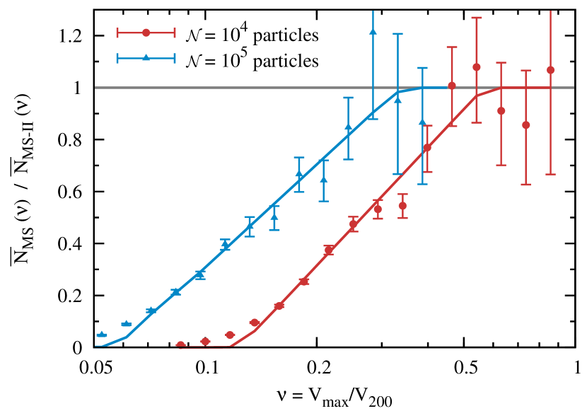
Figure 12: Method A for computing the completeness function. This method compares the subhalo number count, $\overline{N}(\nu)$, in halos of a given mass resolved at two different resolutions in MS and MS-II. The two datasets consist of host halos in the mass range $(0.69-1.1)\times 10^{13}~{}h^{-1}\rm{M}_{\odot}$ (red filled circles) and $(0.6-1.2)\times 10^{14}~{}h^{-1}\rm{M}_{\odot}$ (blue filled triangles). These are resolved in MS with $(0.8-1.2)\times 10^{4}$ and $(0.7-1.3)\times 10^{5}$ particles respectively. The same halos are resolved in MS-II with $125$ times more particles. The two solid lines represent the completeness function fit given by Eqn. (6). The error bars represent the $1\sigma$ uncertainty in the determination of the $\overline{N}_{\mathrm{\textsc{MS}}}(\nu)/\overline{N}_{\mathrm{\textsc{MS-II}}}(\nu)$ ratio.

The simplest way to investigate numerical effects is to compare the subhalo population of halos of a given mass simulated at two different resolutions. For this we use the two Millennium simulations that resolve halos of similar mass with 125 times better resolution in MS-II than in MS. Same mass halos have, on average, $\overline{N}_{\mathrm{\textsc{MS}}}(\nu)$ and $\overline{N}_{\mathrm{\textsc{MS-II}}}(\nu)$ substructures in MS and MS-II respectively. According to Eqn. (5), the ratio of the two subhalo numbers is given by

$$\frac{\overline{N}_{\mathrm{\textsc{MS}}}(\nu)}{\overline{N}_{\mathrm{\textsc{MS-II}}}(\nu)}=\frac{f_{\mathrm{\textsc{MS}}}(\nu)}{f_{\mathrm{\textsc{MS-II}}}(\nu)},$$ (14)

where $f_{\mathrm{\textsc{MS}}}(\nu)$ and $f_{\mathrm{\textsc{MS-II}}}(\nu)$ are the completeness functions for the two Millennium simulations. Because of the higher resolution of MS-II, we can recover the full subhalo population down to lower $\nu$ values than in MS. Thus, this expression can be rewritten as:

$$f_{\mathrm{\textsc{MS}}}(\nu)=\frac{\overline{N}_{\mathrm{\textsc{MS}}}(\nu)}{\overline{N}_{\mathrm{\textsc{MS-II}}}(\nu)},\quad\textrm{as long as}\,\,f_{\mathrm{\textsc{MS-II}}}(\nu)\cong 1.$$ (15)

This holds down to the lowest value of $\nu$ for which MS-II resolves all substructures.

Fig. 12 shows the ratio between the subhalo number counts in the MS and MS-II simulations, for two samples of halos in the mass range $(0.69-1.1)\times 10^{13}~{}h^{-1}\rm{M}_{\odot}$ and $(0.6-1.2)\times 10^{14}~{}h^{-1}\rm{M}_{\odot}$. The lower mass halos are resolved in MS with ${\sim}10^{4}$ particles while the higher mass ones are resolved with ${\sim}10^{5}$ particles. We can see that resolution effects become important at $\nu\approx 0.6$ and $\nu\approx 0.3$ for halos resolved with $10^{4}$ and $10^{5}$ particles. By increasing the number of particles by a factor of $10$, we would resolve the subhalos down to approximately $2$ times lower values of $\nu$. Since MS-II has 125 times higher resolution than MS, it recovers all the subhalos down to ${\sim}4$ times lower $\nu$ than MS, which, according to the figure, corresponds to $\overline{N}_{\mathrm{\textsc{MS}}}(\nu)/\overline{N}_{\mathrm{\textsc{MS-II}}}(\nu)\sim 0.1$. This means that we can use Eqn. (15) to compute $f_{\mathrm{\textsc{MS}}}(\nu)$ as long as $f_{\mathrm{\textsc{MS}{}}}(\nu)\raisebox{-1.29167pt}{\mbox{$\stackrel{{\scriptstyle>}}{{{}_{\sim}}}\,$}}0.1$.

We find that the completeness function given by Eqn. (6) gives a very good fit to the $\overline{N}_{\mathrm{\textsc{MS}}}(\nu)/\overline{N}_{\mathrm{\textsc{MS-II}}}(\nu)$ ratio. This is illustrated by the solid lines in Fig. 12 for halos resolved with $10^{4}$ and $10^{5}$ particles. The fit is a good match to the completeness function for $\nu$ values for which $f(\nu)\geq 0.2$. At lower $\nu$ values the completeness function has a more complex behaviour that is not captured by the two parameter expression that we use. Therefore, we limit our analysis and fits to regions with $f(\nu)\geq 0.2$.

Method A for estimating the completeness function is very simple and straightforward but its simplicity hides a major obvious disadvantage: it requires a second simulation with ${\sim}100$ times higher mass resolution than the original. To overcome this limitation we introduce a different method for computing the completeness function which relies on a single simulation. We use method A to show that this method B gives the same results.

A.2 Method B: comparing low and high mass halos in the same simulation

In a cosmological simulation subhalos are resolved to lower values of $\nu$ in larger halos. Thus, if we assume that the true number of subhalos as function of $\nu$, $\widetilde{N}(\nu)$ (see Eqn. (5)), is self-similar amongst host halos of different mass (see Fig. 9 and Wang12), then we can derive the completeness function by comparing the substructure $\nu$ function in low versus high mass halos.

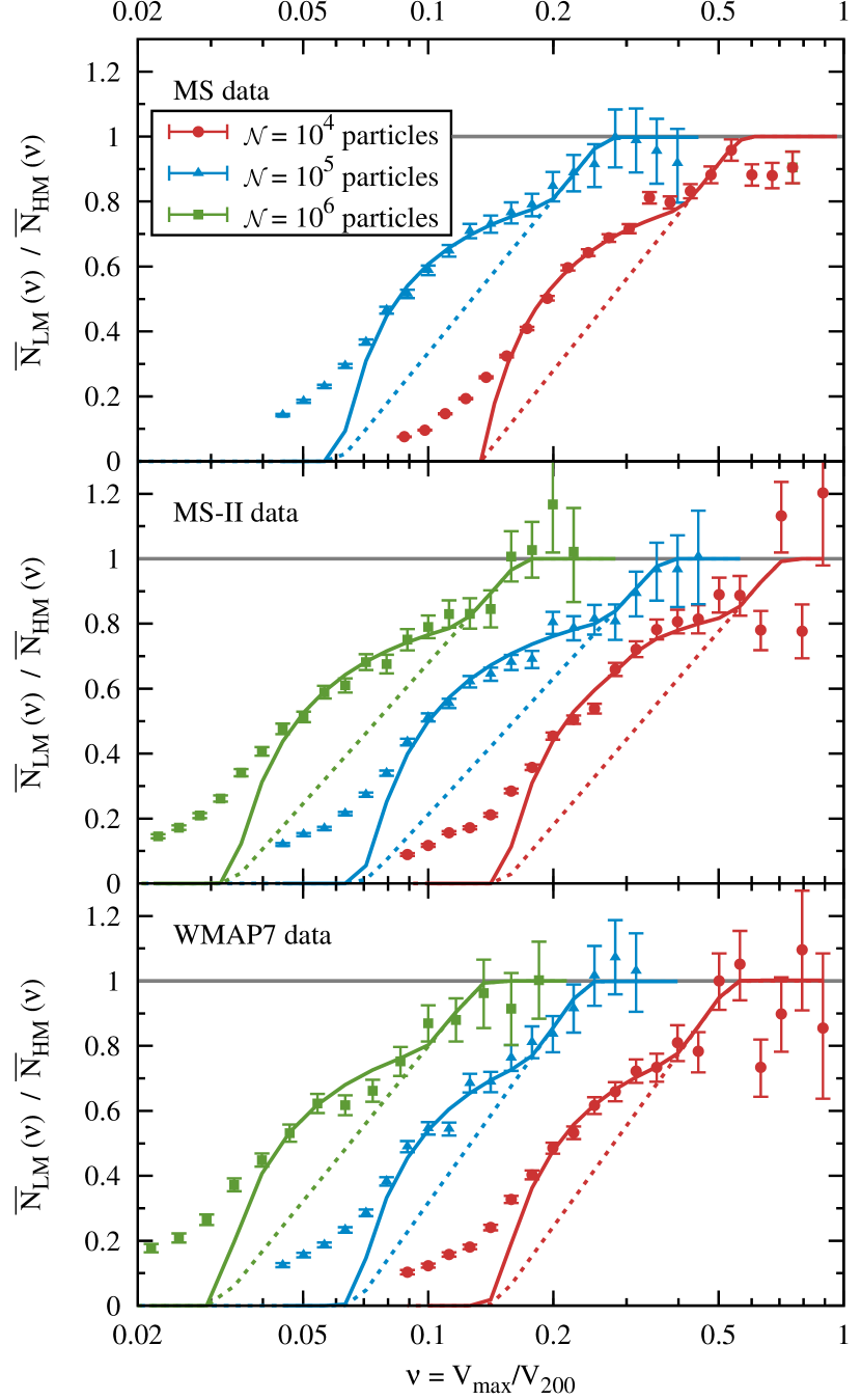
Figure 13: Method B for computing the completeness function for the MS (top panel), MS-II (centre panel) and WMAP7 (bottom panel) simulations. The method uses the ratio of the subhalo abundance, $\overline{N}(\nu){}$, between low-mass (LM) and high-mass (HM) halo samples. The red, blue and green lines and symbols correspond to low-mass halos resolved with $(0.8-1.2)\times 10^{4}$, $(0.8-1.2)\times 10^{5}$ and $(0.8-1.2)\times 10^{6}$ particles in each of the three simulations. The halo mass ranges used for each dataset are given in Table 5. The solid curves represent the fit given by Eqn. (17) to each dataset. The dashed lines show the inferred completeness function, $f_{\mathrm{LM}}(\nu)$, for the low-mass sample. The error bars represent the $1\sigma$ uncertainty in the determination of the $\overline{N}_{\mathrm{LM}}(\nu)/\overline{N}_{\mathrm{HM}}(\nu)$ ratio.

Table 5: The mass range of halos resolved with $\mathcal{N}=(0.8-1.2)\times 10^{4}$, $\mathcal{N}=(0.8-1.2)\times 10^{5}$ and $\mathcal{N}=(0.8-1.2)\times 10^{6}$ particles in the MS, MS-II and WMAP7 simulations. These halo samples were used to obtain the results presented in Fig. 13. We only give the mass range for the low-mass halo sample, since halos in the high-mass sample are always $\Theta=3$ times more massive than these.

Simulation	$\mathcal{N}\sim 10^{4}$	$\mathcal{N}\sim 10^{5}$	$\mathcal{N}\sim 10^{6}$
MS	$(0.68-1.03)\times$	$(0.68-1.03)\times$	-
	$10^{13}~{}h^{-1}\rm{M}_{\odot}$	$10^{14}~{}h^{-1}\rm{M}_{\odot}$
MS-II	$(5.5-8.3)\times$	$(5.5-8.3)\times$	$(5.5-8.3)\times$
	$10^{10}~{}h^{-1}\rm{M}_{\odot}$	$10^{11}~{}h^{-1}\rm{M}_{\odot}$	$10^{12}~{}h^{-1}\rm{M}_{\odot}$
WMAP7	$(5.0-7.5)\times$	$(5.0-7.5)\times$	$(5.0-7.5)\times$
	$10^{10}~{}h^{-1}\rm{M}_{\odot}$	$10^{11}~{}h^{-1}\rm{M}_{\odot}$	$10^{12}~{}h^{-1}\rm{M}_{\odot}$

To illustrate this method we consider two halo samples: a low-mass (LM) and a high-mass (HM) sample. Furthermore, we choose the high-mass halos to be $\Theta$ times more massive than their low-mass counterparts. In the limit when $\widetilde{N}(\nu)$ is independent of host halo mass, the ratio between the number of substructure in the low- and high-mass samples is given by

$$\frac{\overline{N}_{\mathrm{LM}}(\nu)}{\overline{N}_{\mathrm{HM}}(\nu)}=\frac{f_{\mathrm{LM}}(\nu)}{f_{\mathrm{HM}}(\nu)},$$ (16)

where $f_{\mathrm{LM}}(\nu)$ and $f_{\mathrm{HM}}(\nu)$ are the completeness functions of the two halo samples. Using the $f(\nu)$ expression from Eqn. (6), the above relation becomes:

$$\begin{cases}1&\nu_{0}^{\mathrm{LM}}\leq\nu\vspace{.1cm}\\ 1+\alpha^{\mathrm{LM}}\ln\left(\frac{\nu}{\nu_{0}^{\mathrm{LM}}}\right)&\nu_{0}^{\mathrm{HM}}\leq\nu<\nu_{0}^{\mathrm{LM}}\vspace{.2cm}\\ \dfrac{1+\alpha^{\mathrm{LM}}\ln\left(\frac{\nu}{\nu_{0}^{\mathrm{LM}}}\right)}{1+\alpha^{\mathrm{HM}}\ln\left(\frac{\nu}{\nu_{0}^{\mathrm{HM}}}\right)}&\nu_{0}^{\mathrm{LM}}e^{-1/\alpha^{\mathrm{LM}}}\leq\nu<\nu_{0}^{\mathrm{HM}}\vspace{.2cm}\\ 0&\nu<\nu_{0}^{\mathrm{LM}}e^{-1/\alpha^{\mathrm{LM}}},\end{cases}$$ (17)

where $(\nu_{0}^{\mathrm{LM}},\alpha^{\mathrm{LM}})$ and $(\nu_{0}^{\mathrm{HM}},\alpha^{\mathrm{HM}})$ are the completeness function fit parameters corresponding to the low-mass and high-mass halo samples respectively. This expression can be simplified further given that halos in the two samples are resolved with $\mathcal{N}^{\mathrm{LM}}$ and $\mathcal{N}^{\mathrm{HM}}=\Theta\mathcal{N}^{\mathrm{LM}}$ particles. This, combined with the dependence of the fit parameters, $\nu_{0}\propto\mathcal{N}^{n_{\nu}}$ and $\alpha\propto\mathcal{N}^{n_{\alpha}}$, found in Section 3.1, results in

$$\nu_{0}^{\mathrm{HM}}=\nu_{0}^{\mathrm{LM}}\Theta^{n_{\nu}}\mbox{~{}~{}~{}~{}and~{}~{}~{}~{}}\alpha^{\mathrm{HM}}=\alpha^{\mathrm{LM}}\Theta^{n_{\alpha}}\,.$$ (18)

Using these expressions reduces Eqn. (17) to 4 parameters: $\nu_{0}^{\mathrm{LM}}$, $\alpha^{\mathrm{LM}}$, $n_{\nu}$ and $n_{\alpha}$. These fit parameters can be found using the following algorithm:

• Select a value for the mass ratio, $\Theta\sim$ a few.

• Make an initial guess for the parameters $n_{\nu}$ and $n_{\alpha}$.

• Select as the low-mass sample all halos in a chosen mass range. The high-mass sample then contains all halos $\Theta$ times more massive than this. Using these two samples find the best fit values of the parameters $\nu_{0}^{\mathrm{LM}}$ and $\alpha^{\mathrm{LM}}$.

• Repeat the previous step for different host halo masses in order to obtain the parameters $\nu_{0}^{\mathrm{LM}}$ and $\alpha^{\mathrm{LM}}$ for a wide range of halo masses.

• Use the dependence on mass, and therefore on host particle number, $\mathcal{N}$, of $\nu_{0}^{\mathrm{LM}}$ and $\alpha^{\mathrm{LM}}$ found in the previous step to find new values for $n_{\nu}$ and $n_{\alpha}$.

• Check if $n_{\nu}$ and $n_{\alpha}$ have converged to the values used as the input for step (iii). If the values have converged, stop the iterative procedure. Otherwise, repeat steps (iii) through (vi) using the latest values for $n_{\nu}$ and $n_{\alpha}$.

In Fig. 13 we illustrate the use of method B to compute the completeness function for the three N-body simulations used in this study. The figure shows the ratio, $\overline{N}_{\mathrm{LM}}(\nu)/\overline{N}_{\mathrm{HM}}(\nu)$, of the mean number of subhalos in the low- and high-mass halo samples. We plot this ratio for low-mass halos resolved with ${\sim}10^{4}$, ${\sim}10^{5}$ and ${\sim}10^{6}$ particles, with masses given in Table 5. To minimize the variation of the subhalo number counts with mass we take the high-mass sample to be $\Theta=3$ times more massive than the low-mass one. The fit given by Eqn. (17) is shown as a solid curve for each of the datasets. We can see that it gives a very good fit for $\overline{N}_{\mathrm{LM}}(\nu)/\overline{N}_{\mathrm{HM}}(\nu)\geq 0.4$, which corresponds to values $f_{\mathrm{LM}}(\nu)\geq 0.2$, the same limit for which Method A is also accurate.

Fig. 13 shows another important result. The completeness function has the same parametric form, given by Eqn. (6), for all the three simulations used in this study. This is a reflection of the fact that Eqn. (17) gives a very good fit to the $\overline{N}_{\mathrm{LM}}(\nu)/\overline{N}_{\mathrm{HM}}(\nu)$ ratio for the three simulations: MS, MS-II and WMAP7.

Computing the completeness function using method B has the advantage of not requiring a simulation with a higher mass resolution as in method A. This opens up the possibility of quantifying how numerical effects in any given simulation alter the mean subhalo abundance. We illustrated this for MS-II and WMAP7 for which we do not have a higher resolution version and so we cannot apply method A. The main limitation of method B stems from the assumption that the mean subhalo abundance is self-similar amongst host halos of different mass. As we found in Section 5, this condition is satisfied for substructures in dark matter only simulations, but it will not be the case when adding in baryons. The complex feedback processes involved in galaxy formation affect halos of different mass in different ways (eg. Sawala et al., 2013, and references within). This breaks the self-similar behaviour of the subhalo abundance.

Appendix B Comparison of rockstar and subfind subhalo abundances

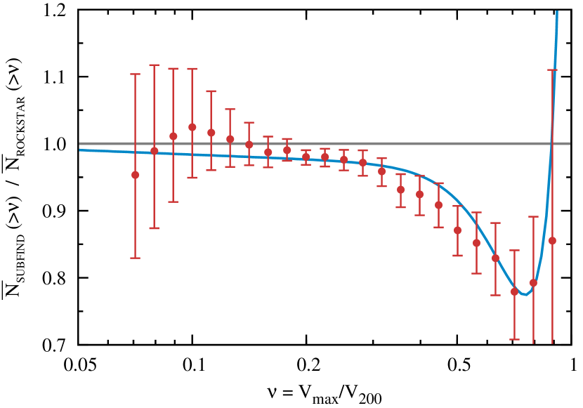
Figure 14: Comparison of the subhalo abundance of galactic mass halos identified with subfind versus that found with rockstar. The points give the $\overline{N}_{\mathrm{\textsc{subfind}}}({>}\nu)/\overline{N}_{\mathrm{\textsc{rockstar}}}({>}\nu)$ ratio as measured in the MS-II. The solid curve shows the ratio between the best fit function (see Eqn. (9)) to the subfind and rockstar subhalo abundance.

Here we investigate if the difference in the subhalo numbers between our analysis and previous studies can be explained by the use of different halo finders. For this, we compare the galactic subhalo abundance as found by rockstar (Behroozi, Wechsler & Wu, 2013) and by subfind (Springel et al., 2001), with the latter used in the studies of Wang12 and BK10.

We apply the same analysis steps to subfind subhalos as we did in the case of rockstar: identify the number of missing substructures due to resolution effects and estimate the true subhalo abundance, following the procedure described in Section 3. The resulting subhalo abundance for MW-mass hosts is well described by Eqn. (9) with best fit parameters: $a=-3.18$, $\nu_{1}=0.333$, $b=6$ and $\nu_{\mathrm{cut}}=0.78$ (for subhalos found within a distance $R_{200}$ from the host). Fig. 14 compares the subhalo abundance found with rockstar and subfind, showing that for $\nu\raisebox{-1.29167pt}{\mbox{$\stackrel{{\scriptstyle<}}{{{}_{\sim}}}\,$}}0.3$ both halo finders get the same number of substructures, up to a few percent difference. For higher $\nu$, subfind identifies ${\sim}10\%$ fewer substructures. Given that such massive subhalos are resolved with $\raisebox{-1.29167pt}{\mbox{$\stackrel{{\scriptstyle>}}{{{}_{\sim}}}\,$}}10^{3}$ particles, the difference is likely due to substructures found close to the centre of the host that are identified by rockstar, which is a phase-space halo finder, and not by subfind, which uses only real-space information. Since Wang12 computed the subhalo abundance only in the interval $0.1\leq\nu\leq 0.5$, the figure clearly shows that the use of rockstar instead of subfind cannot on its own explain the ${\sim}20\%$ higher subhalo abundance found in our study. Similarly, the significantly lower value of the subhalo abundance slope, $a$, found by BK10 is not due to the use of a different halo finder.

References

- Battaglia et al. (2005) Battaglia G. et al., 2005, MNRAS, 364, 433
- Behroozi, Wechsler & Wu (2013) Behroozi P. S., Wechsler R. H., Wu H.-Y., 2013, ApJ, 762, 109
- Benson et al. (2000) Benson A. J., Cole S., Frenk C. S., Baugh C. M., Lacey C. G., 2000, MNRAS, 311, 793
- Benson et al. (2002a) Benson A. J., Frenk C. S., Lacey C. G., Baugh C. M., Cole S., 2002a, MNRAS, 333, 177
- Benson et al. (2002b) Benson A. J., Lacey C. G., Baugh C. M., Cole S., Frenk C. S., 2002b, MNRAS, 333, 156
- Berlind & Weinberg (2002) Berlind A. A., Weinberg D. H., 2002, ApJ, 575, 587
- Boylan-Kolchin, Bullock & Kaplinghat (2011) Boylan-Kolchin M., Bullock J. S., Kaplinghat M., 2011, MNRAS, 415, L40
- Boylan-Kolchin, Bullock & Kaplinghat (2012) Boylan-Kolchin M., Bullock J. S., Kaplinghat M., 2012, MNRAS, 422, 1203
- Boylan-Kolchin et al. (2010) Boylan-Kolchin M., Springel V., White S. D. M., Jenkins A., 2010, MNRAS, 406, 896, (BK10)
- Boylan-Kolchin et al. (2009) Boylan-Kolchin M., Springel V., White S. D. M., Jenkins A., Lemson G., 2009, MNRAS, 398, 1150
- Bullock, Kravtsov & Weinberg (2000) Bullock J. S., Kravtsov A. V., Weinberg D. H., 2000, ApJ, 539, 517
- Busha et al. (2011a) Busha M. T., Marshall P. J., Wechsler R. H., Klypin A., Primack J., 2011a, ApJ, 743, 40
- Busha et al. (2011b) Busha M. T., Wechsler R. H., Behroozi P. S., Gerke B. F., Klypin A. A., Primack J. R., 2011b, ApJ, 743, 117
- Cautun et al. (2014) Cautun M., Frenk C. S., van de Weygaert R., Hellwing W. A., Jones B. J. T., 2014, preprints ArXiv:1405.7697
- Clocchiatti et al. (2006) Clocchiatti A. et al., 2006, ApJ, 642, 1
- Cole et al. (2005) Cole S. et al., 2005, MNRAS, 362, 505
- Davis et al. (1985) Davis M., Efstathiou G., Frenk C. S., White S. D. M., 1985, ApJ, 292, 371
- Dehnen, McLaughlin & Sachania (2006) Dehnen W., McLaughlin D. E., Sachania J., 2006, MNRAS, 369, 1688
- Diemand et al. (2008) Diemand J., Kuhlen M., Madau P., Zemp M., Moore B., Potter D., Stadel J., 2008, Nature, 454, 735
- Dutton & Macciò (2014) Dutton A. A., Macciò A. V., 2014, MNRAS, 441, 3359
- Gao et al. (2011) Gao L., Frenk C. S., Boylan-Kolchin M., Jenkins A., Springel V., White S. D. M., 2011, MNRAS, 410, 2309
- Gao et al. (2004) Gao L., White S. D. M., Jenkins A., Stoehr F., Springel V., 2004, MNRAS, 355, 819
- Garrison-Kimmel et al. (2014) Garrison-Kimmel S., Horiuchi S., Abazajian K. N., Bullock J. S., Kaplinghat M., 2014, preprint ArXiv:1405.3985
- Gnedin et al. (2010) Gnedin O. Y., Brown W. R., Geller M. J., Kenyon S. J., 2010, ApJ, 720, L108
- Guo et al. (2012) Guo Q., Cole S., Eke V., Frenk C., 2012, MNRAS, 427, 428
- Guo et al. (2010) Guo Q., White S., Li C., Boylan-Kolchin M., 2010, MNRAS, 404, 1111
- Guy et al. (2010) Guy J. et al., 2010, A&A, 523, A7
- Jiang & van den Bosch (2014) Jiang F., van den Bosch F. C., 2014, preprints ArXiv:1403.6827
- Karachentsev et al. (2004) Karachentsev I. D., Karachentseva V. E., Huchtmeier W. K., Makarov D. I., 2004, The Astronomical Journal, 127, 2031
- Klypin et al. (1999) Klypin A., Kravtsov A. V., Valenzuela O., Prada F., 1999, ApJ, 522, 82
- Klypin, Trujillo-Gomez & Primack (2011) Klypin A. A., Trujillo-Gomez S., Primack J., 2011, ApJ, 740, 102
- Knebe et al. (2011) Knebe et al., 2011, MNRAS, 415, 2293
- Komatsu et al. (2011) Komatsu et al., 2011, ApJS, 192, 18
- Kravtsov et al. (2004) Kravtsov A. V., Berlind A. A., Wechsler R. H., Klypin A. A., Gottlöber S., Allgood B., Primack J. R., 2004, ApJ, 609, 35
- Li & White (2008) Li Y.-S., White S. D. M., 2008, MNRAS, 384, 1459
- Łokas (2009) Łokas E. L., 2009, MNRAS, 394, L102
- Ma & Fry (2000) Ma C.-P., Fry J. N., 2000, ApJ, 543, 503
- Moore et al. (1999) Moore B., Ghigna S., Governato F., Lake G., Quinn T., Stadel J., Tozzi P., 1999, ApJ, 524, L19
- Moore et al. (1998) Moore B., Governato F., Quinn T., Stadel J., Lake G., 1998, ApJ, 499, L5
- Onions et al (2012) Onions et al, 2012, MNRAS, 423, 1200
- Peñarrubia, McConnachie & Navarro (2008) Peñarrubia J., McConnachie A. W., Navarro J. F., 2008, ApJ, 672, 904
- Peacock & Smith (2000) Peacock J. A., Smith R. E., 2000, MNRAS, 318, 1144
- Piffl et al. (2014) Piffl T. et al., 2014, A&A, 562, A91
- Planck Collaboration (2013) Planck Collaboration, 2013, preprint arXiv:1303.5076
- Purcell & Zentner (2012) Purcell C. W., Zentner A. R., 2012, J. Cosmology Astropart. Phys, 12, 7
- Sakamoto, Chiba & Beers (2003) Sakamoto T., Chiba M., Beers T. C., 2003, A&A, 397, 899
- Sawala et al. (2013) Sawala T., Frenk C. S., Crain R. A., Jenkins A., Schaye J., Theuns T., Zavala J., 2013, MNRAS, 431, 1366
- Scoccimarro et al. (2001) Scoccimarro R., Sheth R. K., Hui L., Jain B., 2001, ApJ, 546, 20
- Seljak (2000) Seljak U., 2000, MNRAS, 318, 203
- Shaw et al. (2006) Shaw L. D., Weller J., Ostriker J. P., Bode P., 2006, ApJ, 646, 815
- Smith et al. (2007) Smith M. C. et al., 2007, MNRAS, 379, 755
- Somerville (2002) Somerville R. S., 2002, ApJ, 572, L23
- Spergel et al. (2003) Spergel et al., 2003, ApJS, 148, 175
- Springel et al. (2008) Springel V. et al., 2008, MNRAS, 391, 1685
- Springel et al. (2005) Springel V. et al., 2005, Nature, 435, 629
- Springel et al. (2001) Springel V., White S. D. M., Tormen G., Kauffmann G., 2001, MNRAS, 328, 726
- Stadel et al. (2009) Stadel J., Potter D., Moore B., Diemand J., Madau P., Zemp M., Kuhlen M., Quilis V., 2009, MNRAS, 398, L21
- Strigari et al. (2008) Strigari L. E., Bullock J. S., Kaplinghat M., Simon J. D., Geha M., Willman B., Walker M. G., 2008, Nature, 454, 1096
- Strigari, Frenk & White (2010) Strigari L. E., Frenk C. S., White S. D. M., 2010, MNRAS, 408, 2364
- Vera-Ciro et al. (2013) Vera-Ciro C. A., Helmi A., Starkenburg E., Breddels M. A., 2013, MNRAS, 428, 1696
- Walker et al. (2009) Walker M. G., Mateo M., Olszewski E. W., Peñarrubia J., Wyn Evans N., Gilmore G., 2009, ApJ, 704, 1274
- Wang et al. (2012) Wang J., Frenk C. S., Navarro J. F., Gao L., Sawala T., 2012, MNRAS, 424, 2715, (Wang12)
- Wang & White (2012) Wang W., White S. D. M., 2012, MNRAS, 424, 2574
- Watkins, Evans & An (2010) Watkins L. L., Evans N. W., An J. H., 2010, MNRAS, 406, 264
- Weinberg et al. (2008) Weinberg D. H., Colombi S., Davé R., Katz N., 2008, ApJ, 678, 6
- Wilkinson & Evans (1999) Wilkinson M. I., Evans N. W., 1999, MNRAS, 310, 645
- Wolf et al. (2010) Wolf J., Martinez G. D., Bullock J. S., Kaplinghat M., Geha M., Muñoz R. R., Simon J. D., Avedo F. F., 2010, MNRAS, 406, 1220
- Xue et al. (2008) Xue X. X. et al., 2008, ApJ, 684, 1143
- Zentner et al. (2005) Zentner A. R., Berlind A. A., Bullock J. S., Kravtsov A. V., Wechsler R. H., 2005, ApJ, 624, 505
- Zheng et al. (2005) Zheng Z. et al., 2005, ApJ, 633, 791