Linear Vlasov Theory in the Shearing Sheet Approximation
with Application to the Magneto-Rotational Instability

Abstract

We derive the conductivity tensor for axisymmetric perturbations of a hot, collisionless, and charge-neutral plasma in the shearing sheet approximation. Our results generalize the well-known linear Vlasov theory for uniform plasmas to differentially rotating plasmas and can be used for wide range of kinetic stability calculations. We apply these results to the linear theory of the magneto-rotational instability (MRI) in collisionless plasmas. We show analytically and numerically how the general kinetic theory results derived here reduce in appropriate limits to previous results in the literature, including the low frequency guiding center (or “kinetic MHD”) approximation, Hall MHD, and the gyro-viscous approximation. We revisit the cold plasma model of the MRI and show that, contrary to previous results, an initially unmagnetized collisionless plasma is linearly stable to axisymmetric perturbations in the cold plasma approximation. In addition to their application to astrophysical plasmas, our results provide a useful framework for assessing the linear stability of differentially rotating plasmas in laboratory experiments.

1 Introduction

The shearing sheet is a widely used model for studying the local dynamics of a differentially rotating disk (e.g. Hill, 1878; Goldreich and Lynden-Bell, 1965; Hawley et al., 1996). The shearing sheet approximation isolates the key local physics of rotating disks, independent of global boundary conditions. Studies of the shearing sheet have provided valuable insight into gravitational instability in galactic and protostellar disks, excitation of shearing waves and spiral structure, and angular momentum transport by turbulence driven by the magneto-rotational instability (MRI).

In studies of self-gravitating stellar systems (in particular, galactic disks) the linear theory of the shearing sheet has been widely developed using both kinetic approaches as well as fluid approximations. However, despite the astrophysical importance of low collisionality ionized accretion flows onto compact objects (Rees et al., 1982; Yuan and Narayan, 2012), there is no existing comprehensive kinetic treatment of the linear theory of a collisionless plasma in the shearing sheet approximation. That is the aim of this paper. In particular, we derive the general conductivity tensor for such a plasma. We then apply this result to study the MRI in kinetic theory.

The analysis in this paper can be viewed as the generalization to a plasma of the previous linear kinetic shearing sheet calculations for self-gravitating stellar systems (e.g. Julian and Toomre, 1966). It is likewise a generalization to a differentially rotating plasma of the standard linear Vlasov theory of uniform plasmas (e.g. Ichimaru, 1973; Krall and Trivelpiece, 1973; Stix, 1992). Moreover, although we specialize to the MRI in the latter part of the paper, our results are likely to be useful for understanding other aspects of differentially rotating plasmas in kinetic theory.

Our study of the MRI in kinetic theory generalizes and extends previous work. In particular, Quataert et al. (2002) studied the MRI in the “kinetic MHD” (or guiding center) approximation, which averages over the cyclotron motion of particles. They also focused solely on kinetic ions, neglecting the electron dynamics under the assumption that the electrons are much colder than the protons. The formalism derived in this paper relaxes both of these restrictions. Our analysis contains as various limits many non-ideal MHD studies of the MRI, in particular those assessing the importance of the Hall effect (Section 5.3.1, Wardle, 1999) and gyro-viscous forces (Section 5.3.2, Ferraro, 2007). We disagree, however, with the cold plasma analysis of Krolik and Zweibel (2006), see Section 4.4.

This paper is organized as follows. We begin by providing a brief overview of kinetic theory in the shearing sheet approximation (Section 2). We then describe in some detail the equilibrium solution of the shearing sheet equations, emphasizing in particular the properties of the equilibrium distribution function (Section 3). Section 4.1 contains the key derivation of the conductivity tensor and the linear dispersion relation in the shearing sheet and shows how those can be derived from standard uniform plasma results in the literature by an appropriate set of coordinate transformations. Sections 4.4 and 5 derive analytically and determine numerically the MRI dispersion relation in various limits and discuss the connection between our results and previous derivations in the literature. Finally, Section 6 summarizes our key results. The Appendices A through D contain various technical aspects of the calculations.

2 Vlasov description of charged particle dynamics in the shearing sheet

The collisionless evolution of charged particles in a rotating frame of reference is described by the Vlasov equation

$$\frac{\partial f_{s}}{\partial t}+\bm{v}\cdot\nabla f_{s}+\frac{e_{s}}{m_{s}}(\bm{E}+\bm{v}\times\bm{B})\cdot\frac{\partial f_{s}}{\partial\bm{v}}-(2\bm{\Omega}\times\bm{v}+\nabla\psi)\cdot\frac{\partial f_{s}}{\partial\bm{v}}=0.$$ (1)

Here, $f_{s}(\bm{r},\bm{v},t)$ is the one-particle distribution function. This is normalized such that the number density $n_{s}$ and bulk velocity $\bm{u}_{s}$ are given by

$$n_{s}=\int d^{3}v\,f_{s}\quad\textrm{and}\quad\bm{u}_{s}=\int d^{3}v\,\bm{v}\hat{f}_{s},$$ (2)

where $\hat{f}_{s}=f_{s}/n_{s}$ is the reduced distribution function.

The tidal potential $\psi$ is the sum of the centrifugal potential and the gravitational potential. In the shearing sheet approximation (Goldreich and Lynden-Bell, 1965), this is given by

$$\psi=-q\Omega^{2}x^{2}+\frac{1}{2}\nu^{2}z^{2}.$$ (3)

The angular velocity $\Omega$ is determined from radial force balance. We assume that in equilibrium, the magnetic field is frozen into a bulk flow $\bm{u}$ common to all species ($\bm{E}+\bm{u}\times\bm{B}=0$). If the gravitational potential is due to a point mass and radial pressure support is negligible, then $q=3/2$ (Keplerian rotation) and the vertical frequency $\nu=\Omega$.

With the tidal potential as given in eq. 3, the dynamics are invariant with respect to translations along $y$. As we will verify below, this implies conservation of canonical angular momentum. On the contrary, there is no invariance with respect to mere translations along $x$. Instead, such translations need to be followed by a Galilean boost along $y$, to wit

$$x\mapsto x+x_{0},\quad y\mapsto y-q\Omega tx_{0},$$ (4)

cf. Wisdom and Tremaine (1988).

3 The steady state

In light of the symmetries discussed in the previous section, we may seek an equilibrium in which the number densities are uniform in $x$ and $y$ and in which the bulk motion of each plasma species is given by

$$\bm{u}=-q\Omega x\bm{e}_{y}.$$ (5)

This shear flow is the local representation of the global differential rotation. We take the magnetic field to be uniform. Ampère’s law $\mu_{0}\bm{J}=\nabla\times\bm{B}$ then implies that the electric current density vanishes, which is consistent with the bulk flow 5 being common to all species. The frozen-in condition gives rise to an electric field $\bm{E}=q\Omega{}x\bm{e}_{y}\times\bm{B}$. Given this, the radial magnetic field $B_{x}$ must vanish according to Ferraro’s theorem (Ferraro, 1937). The equilibrium electromagnetic fields are thus given by

$$\bm{E}=q\Omega xB_{z}\bm{e}_{x}\quad\textrm{and}\quad\bm{B}=B_{y}\bm{e}_{y}+B_{z}\bm{e}_{z}.$$ (6)

Let us now consider the motion of an individual particle with charge-to-mass ratio $e/m$. Given eq. 6, the equation of motion may be written as

$$\frac{d\bm{v}}{dt}=\frac{e}{m}(\bm{E}+\bm{v}\times\bm{B})-(2\bm{\Omega}\times\bm{v}+\nabla\psi)=(\bm{v}+q\Omega x\bm{e}_{y})\times\bm{S}-\nu^{2}z\bm{e}_{z},$$ (7)

where we have introduced the vector

$$\bm{S}=\frac{e}{m}\bm{B}+2\bm{\Omega}.$$ (8)

Note that for neutral particles we recover the equation of motion for test particles in Hill’s approximation (Hill, 1878).

The equation of motion 7 is generated by the Hamiltonian

$$2\mathcal{H}=p_{x}^{2}+{(p_{y}-S_{z}x)}^{2}+{(p_{z}+S_{y}x)}^{2}-q\Omega S_{z}x^{2}+\nu^{2}z^{2},$$ (9)

see appendix A for a derivation. Expressing this in terms of the particle velocity $\bm{v}=\partial\mathcal{H}/\partial\bm{p}$ yields

$$2\mathcal{E}=\bm{v}^{2}-q\Omega S_{z}x^{2}+\nu^{2}z^{2},$$ (10)

which we will refer to as the energy integral or simply the energy. According to Jeans’ theorem, any distribution function that depends only on the integrals of motion is in equilibrium. Thus, any $f(\mathcal{E})$ is in equilibrium. However, any such distribution function describes an equilibrium in which the plasma is not rotationally supported but pressure-supported against the tidal force: there is no mean flow and the density is non-uniform in $x$. An equilibrium distribution function that is compatible with the underlying assumptions of the shearing sheet is obtained as follows.

Inspection of eq. 9 immediately reveals that $y$ is a cyclic coordinate. A second integral of motion (in addition to the energy integral) is thus given by the conjugate momentum $p_{y}$. We will henceforth refer to $p_{y}=v_{y}+S_{z}{}x$ as the (canonical) angular momentum (cf. Wisdom and Tremaine, 1988). For a given $p_{y}$, the dynamics may be described in the reduced phase space $(x,z,p_{x},p_{z}$). A particle traveling in the mid-plane at the local shear velocity 5 corresponds to a stationary point in this reduced phase space. To see this, we note that the first variation of $\mathcal{H}$ is given by

$$\delta\mathcal{H}=v_{x}\delta p_{x}+v_{z}\delta p_{z}+[S_{y}v_{z}-S_{z}(v_{y}+q\Omega x)]\delta x+\nu^{2}z\delta z.$$ (11)

A stationary point is reached if all coefficients in this expression vanish identically. This is the case if and only if

$$z=0\quad\textrm{and}\quad v_{x}=v_{y}+q\Omega x=0.$$ (12)

These orbits are the local representation of global circular orbits (see appendix B). In the following this will be implied and we will refer to them simply as circular orbits.

For a given angular momentum $p_{y}$, the energy of a particle on a circular orbit is

$$2\mathcal{E}_{c}=\frac{p_{y}^{2}}{1-S_{z}/q\Omega}.$$ (13)

Note that $\mathcal{E}_{c}$ depends only on the angular momentum and is thus an integral of motion. We now define the gyration energy $\mathcal{K}=\mathcal{E}-\mathcal{E}_{c}$ as the difference between a particle’s energy and the energy of a hypothetical particle with the same angular momentum but on a circular orbit. The gyration energy is thus

$$2\mathcal{K}=v_{x}^{2}+\frac{{(v_{y}+q\Omega x)}^{2}}{1-\Delta}+v_{z}^{2}+\nu^{2}z^{2},$$ (14)

where we have introduced the tidal anisotropy

$$\Delta=q\Omega/S_{z}.$$ (15)

The gyration energy $\mathcal{K}$ is the natural generalization of the epicyclic energy (Shu, 1969) to charged particles. Inspection of eq. 14 reveals that any distribution function of the form $f(\mathcal{K})$ describes a rotationally supported plasma with a number density uniform in $x$ and $y$ and a bulk flow equal to eq. 5. Note that $\mathcal{K}$ is manifestly positive definite as long as $\Delta<1$. In this case the circular orbit thus minimizes the energy for a given angular momentum. We discuss the case $\Delta\geq 1$ in Section 3.2 below. For now we will assume that $\Delta<1$.

A third integral of motion is easily derived in two important special cases. For a purely vertical magnetic field ($\bm{B}=B_{z}\bm{e}_{z}$), the horizontal degrees of freedom are decoupled from the vertical ones. The corresponding integrals of motion are

$$2\mathcal{K}_{\perp}=v_{x}^{2}+\frac{{(v_{y}+q\Omega x)}^{2}}{1-\Delta}\quad\textrm{and}\quad 2\mathcal{E}_{z}=v_{z}^{2}+\nu^{2}z^{2}.$$ (16)

The inhomogeneity in $z$ can be dealt with using an action-angle formalism (e.g. Kaufman, 1971, 1972).

In the remainder of this paper we will, however, make no assumption about the inclination of $\bm{B}$ in the $yz$-plane but instead assume that $\nu=0$ so that the plasma is homogeneous in $z$. Neglecting stratification is a commonly made simplification that greatly eases the analysis because we may assume that any disturbance of the equilibrium is periodic in $z$. In order to integrate the particle equation of motion in this case, we introduce a new velocity $\bm{\mathring{v}}$ whose components are given by

$$\mathring{v}_{x}=v_{x},\quad\mathring{v}_{y}=\frac{v_{y}+q\Omega x}{\sqrt{1-\Delta}},\quad\mathring{v}_{z}=v_{z}.$$ (17)

Expressed in terms of $\bm{\mathring{v}}$, the equation of motion 7 is

$$d\bm{\mathring{v}}/dt=\bm{\mathring{v}}\times\bm{\omega}_{g},$$ (18)

where the gyro-frequency vector

$$\bm{\omega}_{g}=S_{y}\bm{e}_{y}+S_{z}\sqrt{1-\Delta}\,\bm{e}_{z}.$$ (19)

The gyration energy defined in eq. 14 is simply

$$2\mathcal{K}=\mathring{v}^{2}.$$ (20)

The salient feature of having introduced $\bm{\mathring{v}}$ is that eq. 18 takes the same form as in a uniform plasma, with the gyro-frequency vector $\bm{\omega}_{g}$ defined in eq. 19 playing the role of the cyclotron frequency vector $\bm{\omega}_{c}=e\bm{B}/m$. Let us therefore adopt a cylindrical coordinate system $(\mathring{v}_{\parallel},\mathring{v}_{\perp},\vartheta)$ in $\bm{\mathring{v}}$-space that is aligned with $\bm{\omega}_{g}$. In this and in the following section, the labels $\perp$ and $\parallel$ will always refer to the direction of $\bm{\omega}_{g}$. The steady state Vlasov equation is

$$[(\bm{v}+q\Omega x\bm{e}_{y})\times\bm{S}]\cdot\frac{\partial f}{\partial\bm{v}}=(\bm{\mathring{v}}\times\bm{\omega}_{g})\cdot\frac{\partial f}{\partial\bm{\mathring{v}}}=-\omega_{g}\frac{\partial f}{\partial\vartheta}=0,$$ (21)

where the square of the gyration frequency $\omega_{g}$ is given by

$$\omega_{g}^{2}=S_{y}^{2}+S_{z}(S_{z}-q\Omega).$$ (22)

The equilibrium distribution function is thus gyrotropic in $\bm{\mathring{v}}$-space, i.e. of the form $f(\mathring{v}_{\perp},\mathring{v}_{\parallel})$. For this reason we will refer to $\bm{\mathring{v}}$ as the gyrotropic velocity.

The general form $f(\mathring{v}_{\perp},\mathring{v}_{\parallel})$ includes distribution functions of the form $f(\mathcal{K})$. Such distribution functions are isotropic in $\bm{\mathring{v}}$-space but anisotropic in $\bm{v}$-space (unless $q=0$ or $e/m\to\infty$). This anisotropy is measured by $\Delta$ as defined in eq. 15. It always lies within the orbital plane and is inevitable in the presence of the tidal force, hence the name tidal anisotropy. By contrast, the anisotropy due to different temperatures in the direction parallel and perpendicular to $\bm{\omega}_{g}$ is a free parameter and is distinct from the tidal anisotropy.

3.1 The electromagnetic Schwarzschild distribution

Throughout much of the subsequent analysis we will make no assumptions about the specific form of $f(\mathring{v}_{\perp},\mathring{v}_{\parallel})$. Starting with section Section 4.3 we will, however, assume that the distribution function is given by a Maxwellian in $\bm{\mathring{v}}$-space, to wit

$$f(\mathcal{K})=\frac{n\exp(-\mathcal{K}/v_{t}^{2})}{{(2\pi)}^{3/2}v_{t}^{3}\sqrt{1-\Delta}},$$ (23)

where $v_{t}=\mathrm{const}$ is the thermal velocity. In the guiding center limit ($e/m\to\infty$), this reduces to a drifting Maxwellian in $\bm{v}$-space (as used in e.g. Quataert et al., 2002). Indeed, as $e/m\to\infty$, the tidally induced anisotropy $\Delta\sim{}m/e$ disappears. From the definitions given in eqs. 17 and 19 it then follows that $\bm{\mathring{v}}\approx\bm{v}+q\Omega{}x\bm{e}_{y}$ and $\bm{\omega}_{g}\approx\bm{\omega}_{c}$. In the limit, any distribution function of the form $f(\mathring{v}_{\perp},\mathring{v}_{\parallel})$ thus becomes a drifting gyrotropic distribution in $\bm{v}$-space, with the anisotropy being due to the magnetic field only.

It is also instructive to consider neutral particles ($e=0$). In this case the tidal anisotropy $\Delta=q/2$ and the gyration frequency $\omega_{g}=\kappa$, where $\kappa=\sqrt{2(2-q)}\,\Omega$ is the epicyclic frequency. The distribution function 23 thus reduces to the Schwarzschild distribution (see e.g. Julian and Toomre, 1966). For this reason and for lack of a better name, we will refer to $f(\mathcal{K})$ as given in eq. 23 as the electromagnetic Schwarzschild distribution.

3.2 The case $\Delta>1$

In the above derivation of the equilibrium distribution function we have assumed that the tidal anisotropy $\Delta=q\Omega/S_{z}<1$. We have done so because several quantities are singular if $\Delta=1$. The validity of our analysis is also called into question when $\Delta>1$. In this case the gyration energy is not sign definite, in which case a gyrating particle may reach arbitrarily high velocities for any finite $\mathcal{K}$. One consequence of this is that the electromagnetic Schwarzschild distribution given in eq. 23 is not normalizable unless a seemingly arbitrary cutoff in velocity space is introduced.

What is the significance of $\Delta>1$? To address this question, let us first consider neutral particles. In this case, the tidal anisotropy $\Delta=q/2$ and the condition $\Delta>1$ corresponds to

$$\phantom{\qquad(\textrm{neutral particles})}\kappa^{2}=2(2-q)\Omega^{2}<0\qquad(\textrm{neutral particles}).$$ (24)

We thus recover the familiar Rayleigh criterion. As is well known, circular orbits are unstable if eq. 24 is satisfied. The local manifestation of this is that unperturbed orbits as described by eq. 7 are hyperbolic if $\kappa^{2}<0$. It is doubtful that the shearing sheet approximation can be made sense of in this case. It certainly would not describe the local dynamics of a disk.

The above discussion of neutral particle generalizes straightforwardly to charged particles orbiting in a vertical magnetic field, in which case the analogue of eq. 24 is

$$\phantom{\qquad(\textrm{vertical magnetic field})}\omega_{g}^{2}<0\qquad(\textrm{vertical magnetic field}),$$ (25)

where the gyration frequency is defined in eq. 22. By analogy with the neutral case, we are led to conclude that eq. 25 is the criterion for the motion of a charged particle on a circular orbit to be unstable. In appendix B we shed light on the stability of circular orbits from a global perspective and confirm that this conclusion is indeed correct for particles orbiting in the mid-plane of the disk.

The question of orbital stability becomes more involved if the magnetic field has a toroidal component, in which case the magnetic field is misaligned with the rotation axis. In this case, $\Delta>1$ corresponds to

$$\phantom{\qquad(\textrm{inclined magnetic field})}\omega_{g}^{2}<S_{y}^{2}\qquad(\textrm{inclined magnetic field}),$$ (26)

where we remind the reader that $S_{y}=eB_{y}/m$. Equation 26 says that if the magnetic field has a toroidal component, then there is a region of parameter space, $1<\Delta<1+(S_{y}/S_{z}){}^{2}$, where circular orbits are linearly stable even though they do not minimize the energy. In appendix B we speculate that in spite of eq. 26, circular orbits are destabilized by dissipation if the tidal anisotropy is in the range $1<\Delta<1+(S_{y}/S_{z}){}^{2}$, and that $\Delta<1$ is always the relevant criterion for orbital stability in realistic systems. In the main text we will, however, simply ignore the subtlety associated with this corner case and always take $\Delta<1$.

We finally note that the marginal case $\Delta=1$ corresponds to circular orbits having constant canonical angular momentum. This statement is true regardless of whether the magnetic field is inclined or not, see the global analysis in appendix B. For neutral particles we recover the well known result that circular orbits are stable if the angular momentum is a decreasing function of radius.

4 Linear theory

In this section we calculate the conductivity tensor of a collisionless plasma in the shearing sheet approximation. The conductivity tensor is obtained from the solution of the linearized Vlasov equation and establishes a linear relationship between the perturbed current density and the perturbed electric field. This together with an independent relationship between current and electric field obtained from Maxwell’s equations leads immediately to the dispersion relation of a collisionless plasma.

The calculation of the conductivity tensor of a uniform collisionless plasma is the subject of many textbooks (e.g. Krall and Trivelpiece, 1973; Ichimaru, 1973; Stix, 1992). In generalizing this calculation to the shearing sheet, our strategy will be to manipulate the governing equations in a way that allows us to leverage as many results as possible from the (already tedious) uniform plasma calculation.

Let us first write the dynamical equations, i.e. the Vlasov equation 1 and Faraday’s law $\partial\bm{B}/\partial{}t+\nabla\times\bm{E}=0$, in a form that is manifestly invariant with respect to the Galilean transformation 4. For this we introduce the relative velocity and electric field

$$\tilde{\bm{v}}=\bm{v}+q\Omega x\bm{e}_{y}\quad\textrm{and}\quad\tilde{\bm{E}}=\bm{E}-q\Omega x\bm{e}_{y}\times\bm{B}.$$ (27)

Note that $\tilde{\bm{v}}$ and $\tilde{\bm{E}}$ are the velocity and electric field as seen by an observer that is locally at rest with respect to the background shear flow. Expressed in terms of the relative velocity and electric field, the Vlasov equation is given by

$$\left(\frac{\partial}{\partial t}-q\Omega x\frac{\partial}{\partial y}\right)f_{s}+\tilde{\bm{v}}\cdot\nabla f_{s}+\frac{e_{s}}{m_{s}}(\tilde{\bm{E}}+\tilde{\bm{v}}\times\bm{B})\cdot\frac{\partial f_{s}}{\partial\tilde{\bm{v}}}-(2\bm{\Omega}\times\tilde{\bm{v}}-q\Omega\tilde{v}_{x}\bm{e}_{y}+\nu^{2}z\bm{e}_{z})\cdot\frac{\partial f_{s}}{\partial\tilde{\bm{v}}}=0,$$ (28)

where it is understood that $\partial/\partial{}x$ is now to be evaluated at fixed $\tilde{v}_{y}$. Faraday’s law expressed in terms of $\tilde{\bm{E}}$ may be written as

$$\left(\frac{\partial}{\partial t}-q\Omega x\frac{\partial}{\partial y}\right)\bm{B}+q\Omega B_{x}\bm{e}_{y}+\nabla\times\tilde{\bm{E}}=0.$$ (29)

This form of Faraday’s law makes explicit that the magnetic field is stretched and advected by the background shear.

We note that eqs. 28 and 29 are exact. No approximations have been made so far. We also note that the only explicit $x$-dependence in eqs. 28 and 29 is multiplying $\partial/\partial{}y$. Provided the dynamics are axisymmetric, we may thus take the distribution function $f_{s}$, the magnetic field $\bm{B}$, and the relative electric field $\tilde{\bm{E}}$ to be periodic in $x$.

4.1 The dispersion relation

The conductivity tensor is obtained from the solution of the linearized Vlasov equation

$$\frac{D}{Dt}\delta f_{s}+\frac{e_{s}}{m_{s}}(\delta\tilde{\bm{E}}+\tilde{\bm{v}}\times\delta\bm{B})\cdot\frac{\partial f_{s}}{\partial\tilde{\bm{v}}}=0,$$ (30)

where $D/Dt$ denotes the time derivative along unperturbed orbits discussed in Section 3. The formal solution is given by

$$\delta f_{s}(\bm{r},\tilde{\bm{v}},t)=-\frac{e_{s}}{m_{s}}\int_{-\infty}^{t}\!dt^{\prime}\,[\delta\tilde{\bm{E}}(\bm{r}^{\prime},t^{\prime})+\tilde{\bm{v}}^{\prime}\times\delta\bm{B}(\bm{r}^{\prime},t^{\prime})]\cdot\frac{\partial f_{s}}{\partial\tilde{\bm{v}}^{\prime}}.$$ (31)

This is a so-called orbit integral: $\bm{r}^{\prime}(t^{\prime})$ and $\tilde{\bm{v}}^{\prime}(t^{\prime})$ describe the phase space trajectory of particle on an unperturbed orbit passing through $(\bm{r},\tilde{\bm{v}})$ at time $t$.

From now on we will assume no stratification ($\nu=0$) and axisymmetric disturbances ($\partial/\partial{}y=0$). The dynamical equations then have constant coefficients and we may assume that all disturbances depend on position $\bm{r}$ and time $t$ as $\exp(ik_{x}{}x+ik_{z}{}z-i\omega{}t)$. For such disturbances, Faraday’s law 29 is easily solved for $\delta\bm{B}$, to wit

$$\delta\bm{B}=\frac{\bm{k}}{\omega}\times\left[\left(\mathbf{1}-\frac{q\Omega}{i\omega}\bm{e}_{x}\bm{e}_{y}\right)\cdot\delta\tilde{\bm{E}}\right].$$ (32)

Here, the second term in parentheses arises from the stretching term in eq. 29. Substituting eq. 32 into eq. 31, taking the first moment, multiplying by $e_{s}{}n_{s}$, and summing over species yields the perturbed current density

$$\delta\bm{J}(\bm{r},t)=-\frac{1}{i\omega}\sum_{s}\frac{e_{s}^{2}n_{s}}{m_{s}}\int d^{3}v\,\int_{-\infty}^{t}dt^{\prime}\tilde{\bm{v}}\frac{\partial\hat{f}_{s}}{\partial\tilde{\bm{v}}^{\prime}}\cdot\big{[}i(\omega-\bm{k}\cdot\tilde{\bm{v}}^{\prime})\mathbf{1}+i\bm{k}\tilde{\bm{v}}^{\prime}+q\Omega\bm{e}_{x}\bm{e}_{y}\big{]}\cdot\left(\mathbf{1}-\frac{q\Omega}{i\omega}\bm{e}_{x}\bm{e}_{y}\right)\cdot\delta\tilde{\bm{E}}(\bm{r}^{\prime},t^{\prime}),$$ (33)

where $\hat{f}_{s}=f_{s}/n_{s}$ is the reduced distribution function.

Equation 33 establishes a linear relationship between $\delta\bm{J}$ and $\delta\tilde{\bm{E}}$. For this relation to be useful we need to carry out the orbit integral. Inspection of the unperturbed equations of motion might give the impression that in the shearing sheet approximation, this is a more complicated task than in a uniform plasma. However, we have seen in the previous section that the equilibrium orbits closely resemble those in a uniform plasma when expressed in terms of the gyrotropic velocity $\bm{\mathring{v}}$ defined in eq. 17. This suggests that we try to express eq. 33 solely in terms of $\bm{\mathring{v}}$. In appendix C we show that this yields

$$\delta\bm{J}=-\frac{1}{i\omega}\sum_{s}\frac{e_{s}^{2}n_{s}}{m_{s}}\left(\mathbf{Q}_{s}\cdot\mathbf{\Lambda}_{s}\cdot\mathbf{Q}_{s}+\Delta_{s}\bm{e}_{y}\bm{e}_{y}\right)\cdot\left(\mathbf{1}-\frac{q\Omega}{i\omega}\bm{e}_{x}\bm{e}_{y}\right)\cdot\delta\tilde{\bm{E}},$$ (34)

where the response tensor

$$\mathbf{\Lambda}_{s}=\int d^{3}v\int_{0}^{\infty}d\tau\,\bm{\mathring{v}}\frac{\partial\hat{f}_{s}}{\partial\bm{\mathring{v}}^{\prime}}\cdot[i(\omega-\bm{k}\cdot\bm{\mathring{v}}^{\prime})\mathbf{1}+i\bm{k}\bm{\mathring{v}}^{\prime}]\exp\{i\bm{k}\cdot(\bm{r}^{\prime}-\bm{r})+i\omega\tau\}$$ (35)

with $\tau=t-t^{\prime}$. Here, $\Delta_{s}=q\Omega/(\omega_{cs}{}b_{z}+2\Omega)$ is the tidal anisotropy, with both $\omega_{cs}=e_{s}{}B/m_{s}$ and $b_{z}$ being signed quantities. The anisotropy tensor $\mathbf{Q}_{s}$ in eq. 34 is given by

$$\mathbf{Q}_{s}=\bm{e}_{x}\bm{e}_{x}+\bm{e}_{y}\bm{e}_{y}\sqrt{1-\Delta_{s}}+\bm{e}_{z}\bm{e}_{z}.$$ (36)

While everything to the left of $\delta\tilde{\bm{E}}$ on the right hand side of eq. 34 could rightfully be referred to as the shearing sheet conductivity tensor, we choose to define this as

$$\bm{\sigma}=-\frac{1}{i\omega}\sum_{s}\frac{e_{s}^{2}n_{s}}{m_{s}}\mathbf{Q}_{s}\cdot\mathbf{\Lambda}_{s}\cdot\mathbf{Q}_{s}.$$ (37)

Defined in this way, it most closely resembles the uniform plasma conductivity tensor (see e.g. Ichimaru, 1973).

We are now in a position to write down the general dispersion relation of a charge-neutral collisionless plasma in the shearing sheet approximation. Inserting the solution of Faraday’s law given in eq. 32 into Ampère’s law $\mu_{0}\delta\bm{J}=i\bm{k}\times\delta\bm{B}$ (neglecting the displacement current), and eliminating the perturbed current using eq. 34 yields

$$\mathbf{D}\cdot\left(\mathbf{1}-\frac{q\Omega}{i\omega}\bm{e}_{x}\bm{e}_{y}\right)\cdot\delta\tilde{\bm{E}}=0,$$ (38)

where the dispersion tensor

$$\mathbf{D}=(k^{2}\mathbf{1}-\bm{k}\bm{k}-i\omega\mu_{0}\bm{\sigma})v_{a}^{2}-2q\Omega^{2}\sum_{s}\frac{n_{s}m_{s}}{\rho}\frac{\omega_{cs}/b_{z}}{\omega_{cs}b_{z}+2\Omega}\bm{e}_{y}\bm{e}_{y}.$$ (39)

Here, $\rho=\sum_{s}{}n_{s}{}m_{s}$ is the mass density, $v_{a}^{2}=B^{2}/\mu_{0}\rho$ is the square of the Alfvén speed, and we have used the charge-neutrality condition to rewrite the last term on the right hand side.

4.2 The plasma response

From now on we will suppress the species index when there is no risk of confusion. As promised earlier, the orbit integral in eq. 35 only involves the gyrotropic velocity. Let us adopt a right-handed Cartesian coordinate system $(\bm{e}_{1},\bm{e}_{2},\bm{e}_{3})$ with $\bm{e}_{3}=\bm{\omega}_{g}/\omega_{g}$. The unperturbed orbit in $\bm{\mathring{v}}$-space is then simply

$$\bm{\mathring{v}}^{\prime}=\mathring{v}_{\perp}[\bm{e}_{1}\cos(\vartheta+\omega_{g}\tau)+\bm{e}_{2}\sin(\vartheta+\omega_{g}\tau)]+\mathring{v}_{\parallel}\bm{e}_{3}.$$ (40)

The gyro-frequency has no component along the $x$-direction. Thus we may write

$$\bm{e}_{3}=\bm{e}_{z}\cos\varphi-\bm{e}_{y}\sin\varphi.$$ (41)

The orientation of the coordinate axes in the plane perpendicular to $\bm{\omega}_{g}$ is arbitrary at this point. We can exploit this freedom by choosing a frame in which the wave vector $\bm{k}=k_{x}\bm{e}_{x}+k_{z}\bm{e}_{z}$ lies in the plane spanned by $\bm{e}_{1}$ and $\bm{e}_{3}$. The desired orientation of the basis vectors is achieved if $\bm{e}_{1}$ and $\bm{e}_{2}$ are defined through

$$k_{\perp}\bm{e}_{1}=k_{x}\bm{e}_{x}+k_{z}\sin\varphi\,\bm{e}_{3}\times\bm{e}_{x}$$ (42)

and $\bm{e}_{2}=\bm{e}_{3}\times\bm{e}_{1}$. Indeed, projecting the wave vector onto the new basis shows that $\bm{k}=k_{\perp}\bm{e}_{1}+k_{\parallel}\bm{e}_{3}$, where the perpendicular and parallel wave number are given by

$$k_{\perp}^{2}=k_{x}^{2}+k_{z}^{2}\sin^{2}\varphi\quad\textrm{and}\quad k_{\parallel}=k_{z}\cos\varphi,$$ (43)

respectively. In the following we will refer to the coordinate basis defined by eqs. 41 and 42 and illustrated in fig. 1 as the Stix basis.

Figure 1: Illustration of the coordinate transformations 41 and 42 used in calculating the plasma response tensor 45. The $(x,y,z)$-coordinate frame is the standard shearing sheet coordinate frame. The gyro-frequency vector $\bm{\omega}_{g}$ defines the $3$-axis of the $(1,2,3)$-coordinate frame that we refer to as the Stix frame. The $1$-axis is rotated with respect to the $x$-axis by an angle $\chi$ about the $3$-axis, which in turn is inclined with respect to the $z$-axis by an angle $\varphi$ about the $x$-axis. The two Euler angles $\varphi$ and $\chi$ are related through $k_{x}\tan\chi=k_{z}\sin\varphi$.

In order to determine the particle orbit in position space, we note that for axisymmetric disturbances it follows from eq. 17 that $\bm{k}\cdot{}d\bm{r}^{\prime}/dt^{\prime}=\bm{k}\cdot\bm{v}^{\prime}=\bm{k}\cdot\bm{\mathring{v}}^{\prime}$. Working in the Stix basis, it is easy to see that integrating this equation subject to the condition $\bm{r}^{\prime}(t)=\bm{r}$ yields

$$\bm{k}\cdot(\bm{r}-\bm{r}^{\prime})=\frac{k_{\perp}\mathring{v}_{\perp}}{\omega_{g}}[\sin(\vartheta+\omega_{g}\tau)-\sin\vartheta]+k_{\parallel}\mathring{v}_{\parallel}\tau.$$ (44)

With this we can now carry out the integrals over $\tau$ and the gyro-phase $\vartheta$ in eq. 35. This calculation is entirely analogous to the corresponding calculation in a uniform plasma (see e.g. Ichimaru, 1973) modulo the substitutions $(v_{\perp},v_{\parallel},\omega_{cs})\to(\mathring{v}_{\perp},\mathring{v}_{\parallel},\omega_{gs})$. The result may be written as

$$\mathbf{\Lambda}=\mathbf{1}+\sum_{n=-\infty}^{\infty}\int d^{3}v\left(\frac{n\omega_{g}}{\mathring{v}_{\perp}}\frac{\partial\hat{f}}{\partial\mathring{v}_{\perp}}+k_{\parallel}\frac{\partial\hat{f}}{\partial\mathring{v}_{\parallel}}\right)\frac{\mathbf{\Pi}_{n}(\mathring{v}_{\perp},\mathring{v}_{\parallel})}{n\omega_{g}+k_{\parallel}\mathring{v}_{\parallel}-\omega}.$$ (45)

In the Stix basis ($\bm{e}_{1},\bm{e}_{2},\bm{e}_{3}$), the tensors $\mathbf{\Pi}_{n}$ have the matrix representation

$$\mathbf{\Pi}_{n}(\mathring{v}_{\perp},\mathring{v}_{\parallel})\doteq\left[\begin{matrix}\dfrac{n^{2}\omega_{g}^{2}}{k_{\perp}^{2}}J_{n}^{2}&i\mathring{v}_{\perp}\dfrac{n\omega_{g}}{k_{\perp}}J_{n}J_{n}^{\prime}&\mathring{v}_{\parallel}\dfrac{n\omega_{g}}{k_{\perp}}J_{n}^{2}\\ -i\mathring{v}_{\perp}\dfrac{n\omega_{g}}{k_{\perp}}J_{n}J_{n}^{\prime}&\mathring{v}_{\perp}^{2}J_{n}^{\prime 2}&-i\mathring{v}_{\parallel}\mathring{v}_{\perp}J_{n}J_{n}^{\prime}\\ \mathring{v}_{\parallel}\dfrac{n\omega_{g}}{k_{\perp}}J_{n}^{2}&i\mathring{v}_{\parallel}\mathring{v}_{\perp}J_{n}J_{n}^{\prime}&\mathring{v}_{\parallel}^{2}J_{n}^{2}\end{matrix}\right],$$ (46)

where $J_{n}$ is the Bessel function of order $n$. Its argument is $k_{\perp}\mathring{v}_{\perp}/\omega_{g}$ and $J_{n}^{\prime}$ denotes the derivative with respect to said argument.

We stress that all we have assumed in deriving eqs. 45 and 46 is $k_{y}=0$. In order to carry out the remaining integrations over $\mathring{v}_{\perp}$ and $\mathring{v}_{\parallel}$ in eq. 45, we need to specify the particular form of the distribution function $f(\mathring{v}_{\perp},\mathring{v}_{\parallel})$. In the next section we will carry out this calculation for the electromagnetic Schwarzschild distribution defined in eq. 23.

4.3 Response tensor for the electromagnetic Schwarzschild distribution

The result given in eq. 45 holds for general equilibrium distribution functions of the form $f(\mathring{v}_{\perp},\mathring{v}_{\parallel})$. We now specialize to the electromagnetic Schwarzschild distribution defined in eq. 23 and given by

$$f(\mathcal{K})=\frac{n\exp(-\mathcal{K}/v_{t}^{2})}{{(2\pi)}^{3/2}v_{t}^{3}\sqrt{1-\Delta}},$$ (47)

where $v_{t}=\mathrm{const}$ is the thermal velocity. We remind the reader that the tidal anisotropy $\Delta=q\Omega/(\omega_{c}{}b_{z}+2\Omega)$ and the gyration energy

$$\mathcal{K}=\frac{1}{2}\left[v_{x}^{2}+\frac{{(v_{y}+q\Omega x)}^{2}}{1-\Delta}+v_{z}^{2}\right]=\frac{\mathring{v}^{2}}{2}.$$ (48)

The second equality shows that we are simply considering a plasma that is Maxwellian in $\bm{\mathring{v}}$-space.

Given the equilibrium distribution function in eq. 47, the integrals over $\mathring{v}_{\perp}$ and $\mathring{v}_{\parallel}$ that appear in the response tensor 45 can now be performed. This calculation is again entirely analogous to the corresponding calculation in a uniform plasma (see e.g. Ichimaru, 1973). We may thus spare the reader the details and simply state the result

$$\mathbf{\Lambda}=\sum_{n=-\infty}^{\infty}\frac{\zeta_{0}}{\zeta_{n}}\{1-W(\zeta_{n})\}\mathbf{T}_{n}-\zeta_{0}^{2}\bm{e}_{3}\bm{e}_{3},$$ (49)

where

$$\zeta_{n}=\frac{\omega-n\omega_{g}}{|k_{\parallel}|v_{t}}.$$ (50)

The $W$-function used here and in Ichimaru (1973) is related to the standard plasma dispersion function $Z$ defined by Fried and Conte (1961) through $W(\zeta)=1+\xi{}Z(\xi)$ with $\zeta=\sqrt{2}\,\xi$. In the Stix basis, the tensors $\mathbf{T}_{n}$ in eq. 49 have the matrix representation

$$\mathbf{T}_{n}\doteq\left[\begin{matrix}\dfrac{n^{2}}{\lambda}\Gamma_{n}&in\Gamma_{n}^{\prime}&\dfrac{k_{\parallel}}{|k_{\parallel}|}\dfrac{n}{\sqrt{\lambda}}\,\zeta_{n}\Gamma_{n}\\ -in\Gamma_{n}^{\prime}&\dfrac{n^{2}}{\lambda}\Gamma_{n}-2\lambda\Gamma_{n}^{\prime}&-i\dfrac{k_{\parallel}}{|k_{\parallel}|}\sqrt{\lambda}\,\zeta_{n}\Gamma_{n}^{\prime}\\ \dfrac{k_{\parallel}}{|k_{\parallel}|}\dfrac{n}{\sqrt{\lambda}}\,\zeta_{n}\Gamma_{n}&i\dfrac{k_{\parallel}}{|k_{\parallel}|}\sqrt{\lambda}\,\zeta_{n}\Gamma_{n}^{\prime}&\zeta_{n}^{2}\Gamma_{n}\end{matrix}\right].$$ (51)

Here, the $\Gamma_{n}$ are related to the modified Bessel functions of the first kind $I_{n}$ through

$$\Gamma_{n}(\lambda)=I_{n}(\lambda)\exp(-\lambda).$$ (52)

Their argument in eq. 51 is

$$\lambda=\frac{k_{\perp}^{2}v_{t}^{2}}{\omega_{g}^{2}}.$$ (53)

4.4 Cold plasma limit

The cold plasma conductivity tensor may be obtained from the results of the previous section by letting $v_{t}\to 0$. In this limit we may drop all $W$-functions in eq. 49, since $\zeta_{n}\to\infty$, and most of the $\Gamma_{n}$ in eq. 51, since $\lambda\to 0$. We are then left with the response tensor

$$\mathbf{\Lambda}_{s}=\bm{e}_{3}\bm{e}_{3}+\frac{1}{2}\sum_{\pm}\frac{\omega}{\omega\pm\omega_{gs}}(\bm{e}_{1}\pm i\bm{e}_{2})(\bm{e}_{1}\mp i\bm{e}_{2}).$$ (54)

The response tensor is singular for $\omega^{2}=\omega_{gs}^{2}$. This can be understood as follows. The linearized cold plasma momentum equation in the presence of Coriolis and tidal forces is

$$\left(\frac{\partial}{\partial t}-q\Omega x\frac{\partial}{\partial y}+2\bm{\Omega}\times\mathbf{1}-q\Omega\bm{e}_{y}\bm{e}_{x}\right)\cdot\delta\tilde{\bm{u}}_{s}=\frac{e_{s}}{m_{s}}(\delta\tilde{\bm{E}}+\delta\tilde{\bm{u}}_{s}\times\bm{B}).$$ (55)

Multiplying this with $n_{s}{}m_{s}$, summing over species, assuming axisymmetric perturbations, and using charge-neutrality yields

$$\sum_{s}\left[-i\omega\mathbf{1}+\left(2\bm{\Omega}+\frac{e_{s}}{m_{s}}\bm{B}\right)\times\mathbf{1}-q\Omega\bm{e}_{y}\bm{e}_{x}\right]\cdot n_{s}m_{s}\delta\tilde{\bm{u}}_{s}=0.$$ (56)

This equation has a non-trivial solution (with at least one $\delta\tilde{\bm{u}}_{s}\neq 0$) if the tensor in square brackets is singular, i.e. if

$$i\omega(\omega^{2}-\omega_{gs}^{2})=0,$$ (57)

where the square of the gyration frequency $\omega_{gs}$ is defined in eq. 22.

The response tensor in eq. 54 is derived by expressing the perturbed current in terms of the perturbed electric field, which requires inverting the tensor in square brackets in eq. 56. The apparent singularity in the plasma response at $\omega^{2}=\omega_{gs}^{2}$ is a consequence of this inversion being possible only if said tensor is non-singular, i.e. if $\omega^{2}\neq\omega_{gs}^{2}$. In what follows we will thus assume that $\omega^{2}\neq\omega_{gs}^{2}$.

Combining eqs. 37, 39 and 54 leads to the dispersion relation of a cold multicomponent plasma in the shearing sheet approximation. The dynamics of such a plasma were studied previously by Krolik and Zweibel (2006). We disagree with their analysis for the following reasons. First, they have an incorrect expression for the gyration frequency, which can be read off from the denominator of their eq. (3), which disagrees with our eq. 22. Second, their dispersion relation does not reproduce the Hall MRI dispersion relation (Wardle, 1999; Balbus and Terquem, 2001) in the limit $m_{e}\to 0$, as it should (and as our dispersion relation does, see Section 5.3.1 below). Finally, Krolik and Zweibel (2006) claim that a differentially rotating, cold, and initially unmagnetized plasma is linearly unstable with a growth rate comparable to the rotation frequency. We will now show that this is in fact not the case.

4.4.1 Zero magnetization

Here we consider the stability of an initially unmagnetized cold plasma in the shearing sheet. The dispersion relation for this case is obtained from the general expression eq. 39 together with eq. 37 by substituting eq. 54 and then letting the magnetic field strength tend to zero. The dispersion tensor in this limit reduces to

$$v_{a}^{-2}\ell^{2}\mathbf{D}=(k^{2}\mathbf{1}-\bm{k}\bm{k}-i\omega\mu_{0}\bm{\sigma})\ell^{2}+q/2\,\bm{e}_{y}\bm{e}_{y},$$ (58)

where $\ell$ is the mean inertial length, defined through

$$\ell^{-2}=\mu_{0}\sum_{s}\frac{e_{s}^{2}n_{s}}{m_{s}}.$$ (59)

The limiting form of the cold plasma conductivity tensor is

$$-i\omega\mu_{0}\bm{\sigma}=\ell^{-2}\mathbf{Q}\cdot\mathbf{\Lambda}\cdot\mathbf{Q},$$ (60)

where the anisotropy tensor is given in eq. 36 with $\Delta_{s}=q/2$ and the cold plasma response tensor for $B=0$ is

$$\mathbf{\Lambda}=\bm{e}_{z}\bm{e}_{z}+\frac{1}{2}\sum_{\pm}\frac{\omega}{\omega\pm\kappa}(\bm{e}_{x}\pm i\bm{e}_{y})(\bm{e}_{x}\mp i\bm{e}_{y}).$$ (61)

With this, setting the determinant of eq. 58 equal to zero yields the dispersion relation

$$\frac{\omega^{2}{(1+k^{2}\ell^{2})}^{2}-\kappa^{2}k_{z}^{2}\ell^{2}(q/2+k^{2}\ell^{2})}{\omega^{2}-\kappa^{2}}=0.$$ (62)

Assuming $\omega^{2}\neq\kappa^{2}$, the solution is

$$\omega^{2}=\frac{\kappa^{2}k_{z}^{2}\ell^{2}(q/2+k^{2}\ell^{2})}{{(1+k^{2}\ell^{2})}^{2}}.$$ (63)

This is manifestly positive as long as $q>0$. Thus there is no instability as long as the orbital frequency decreases radially outward.

5 The kinetic MRI with finite ion cyclotron frequency

5.1 Cold and massless electrons

In most plasmas, electrons are much lighter than ions, and so the mass ratio $m_{e}/m_{i}\ll 1$. If we assume that the electrons are also much colder than the ions ($T_{e}/T_{i}\ll 1$), then the electrons can be modeled as a cold massless fluid. Expanding the cold electron conductivity tensor in the mass ratio yields

$$\bm{\sigma}_{e}\approx-\frac{1}{i\omega}\frac{e^{2}n_{e}}{m_{e}}\bm{b}\bm{b}+\frac{en_{e}}{B}\bm{b}\times\mathbf{1},$$ (64)

where we have dropped terms of order $m_{e}/m_{i}$ and higher. The first term evidently diverges as the mass ratio goes to zero. Because this term is proportional to $\bm{b}\bm{b}$, the dispersion tensor becomes block-diagonal. In the cold and massless electron limit, the dispersion relation thus factorizes into $\delta{}\tilde{E}_{\parallel}=0$ and $\det\mathbf{D}_{\perp}=0$, where the perpendicular dispersion tensor

$$\mathbf{D}_{\perp}={(k^{2}\mathbf{1}-\bm{k}\bm{k}-i\omega\mu_{0}\bm{\sigma}_{i})}_{\perp}v_{a}^{2}-i\omega\bar{\omega}_{c}\bm{b}\times\mathbf{1}-2q\Omega^{2}\sum_{s}\frac{n_{s}{}m_{s}}{\rho}\frac{\omega_{cs}b_{z}}{\omega_{cs}b_{z}+2\Omega}(\bm{b}\times\bm{e}_{x})(\bm{b}\times\bm{e}_{x}).$$ (65)

We note that throughout this section, the labels $\perp$ and $\parallel$ refer to the direction of $\bm{b}$, not to the gyro-frequency vector $\bm{\omega}_{g}$ as in Sections 3 and 4. In eq. 65, $\bm{\sigma}_{i}$ is the (multi-component) ion conductivity tensor and

$$\bar{\omega}_{c}=\frac{en_{e}B}{\rho}=\sum_{s}\frac{n_{s}m_{s}}{\rho}\omega_{cs}$$ (66)

is the (mass density weighted) mean ion cyclotron frequency.

In appendix D we derive the dispersion relation of a so-called Vlasov-fluid in the shearing sheet. Vlasov-fluid theory (Freidberg, 1972) assumes that the electrons are massless and isotropic, but not necessarily cold. The dispersion relation derived above agrees with the Vlasov-fluid dispersion relation for $T_{e}=0$, see eq. 150.

In the remainder of this section we will assume that there is only one ion species. The perpendicular dispersion tensor in this case is given by

$$\mathbf{D}_{\perp}=v_{a}^{2}{(k^{2}\mathbf{1}-\bm{k}\bm{k})}_{\perp}+\omega_{c}^{2}{(\mathbf{Q}\cdot\mathbf{\Lambda}\cdot\mathbf{Q})}_{\perp}-i\omega\omega_{c}\bm{b}\times\mathbf{1}-2q\Omega^{2}\omega_{c}b_{z}/S_{z}(\bm{b}\times\bm{e}_{x})(\bm{b}\times\bm{e}_{x}).$$ (67)

We focus on the Vlasov-fluid limit in this section to make contact with the existing kinetic theory calculations of the MRI, all of which have assumed cold electrons. We stress, however, that the results derived in the previous section are fully general and can be used to quantify the effects of kinetic electrons on the MRI. The cold electron approximation used here and in previous studies formally requires that $\zeta_{n}\rightarrow\infty$ for all $n$ (Section 4.4). However, $\zeta_{0}=\omega/|k_{\parallel}|v_{te}\sim{}v_{a}/v_{te}$ for the MRI (taking $\omega\sim{}k_{\parallel}v_{a}$). Thus $\zeta_{0}\gg{}1$ requires $T_{e}/T_{i}\ll(m_{e}/m_{i})\beta_{i}^{-1}$. This is in general not satisfied so that the cold electron approximation is not formally applicable when studying the MRI in hot accretion flows. In future work, we will study the effect of (hot) kinetic electrons on the MRI in collisionless plasmas.

5.2 The guiding center limit

In the limit $e/m\to\infty$ we should be able to recover the results of Quataert et al. (2002) who analyzed the stability of a differentially rotating plasma in the shearing sheet approximation using the so-called kinetic MHD equations (see e.g. Grad, 1961; Kulsrud, 1983; Hazeltine and Waelbroeck, 2004). We start by expanding the response tensor in powers of $m/e$. Keeping mostly leading order terms, this yields

$$\mathbf{\Lambda}\approx-\frac{\omega^{2}}{\omega_{c}^{2}}(\mathbf{1}-\bm{e}_{3}\bm{e}_{3})+\frac{i\omega}{\omega_{c}}\left[1-\frac{(4-q)\Omega b_{z}}{2\omega_{c}}\right]\bm{e}_{3}\times\mathbf{1}-\frac{2(W-1)k_{\perp}^{2}v_{t}^{2}}{\omega_{c}^{2}}\bm{e}_{2}\bm{e}_{2}+\frac{i\zeta_{0}Wk_{\perp}v_{t}}{\omega_{c}}\bm{e}_{1}\times\mathbf{1}-\zeta_{0}^{2}W\bm{e}_{3}\bm{e}_{3}.$$ (68)

The argument of the $W$-function is $\zeta_{0}=\omega/|k_{\parallel}|v_{t}$. Expanding the anisotropy tensor $\mathbf{Q}$ yields

$$\mathbf{Q}\approx\mathbf{1}-\frac{q\Omega}{2\omega_{c}b_{z}}\left[1-\frac{(8-q)\Omega}{4\omega_{c}b_{z}}\right]\bm{e}_{y}\bm{e}_{y}.$$ (69)

In order to derive the guiding center limit of the perpendicular dispersion tensor given in eq. 67, we need to compute the tensor product $\mathbf{Q}\cdot\mathbf{\Lambda}\cdot\mathbf{Q}$ and project the result onto the plane orthogonal to the magnetic field. Doing so is complicated by the fact that for finite $e/m$ and $B_{y}\neq{}0$, the magnetic field and the gyro-frequency vector $\bm{\omega}_{g}=\omega_{g}\bm{e}_{3}$ are misaligned, see fig. 1. This makes taking the limit $e/m\to\infty$ a tedious (albeit straightforward) task. At the end of the day, the matrix representation of the perpendicular dispersion tensor 67 in the basis $(\bm{e}_{x},\bm{b}\times\bm{e}_{x})$ is, however, given by the relatively compact expression

$$\lim_{e/m\to\infty}\mathbf{D}_{\perp}\doteq\Bigg{[}\begin{matrix}k_{\parallel}^{2}v_{a}^{2}-\omega^{2}&2i\omega\Omega b_{z}(1+Wb_{y}^{2}/b_{z}^{2})\\ -2i\omega\Omega b_{z}(1+Wb_{y}^{2}/b_{z}^{2})&k_{\parallel}^{2}v_{a}^{2}-\omega^{2}-2q\Omega^{2}-4\Omega^{2}b_{y}^{2}\zeta_{0}^{2}W\end{matrix}\Bigg{]}+v_{a}^{2}\{1+\beta(1-W)\}\Bigg{[}\begin{matrix}k_{z}^{2}b_{y}^{2}&k_{x}k_{z}b_{y}\\ k_{x}k_{z}b_{y}&k_{x}^{2}\end{matrix}\Bigg{]},$$ (70)

where $\beta=2v_{t}^{2}/v_{a}^{2}$. Figure 2 shows plots of the resulting dispersion relation $\det\mathbf{D}_{\perp}=0$ for different values of $\beta_{z}=\beta/b_{z}^{2}$. The results are in good agreement with Figs. 3 and 4 of Quataert et al. (2002). The physics of the MRI in the guiding center limit are discussed in detail in Quataert et al. (2002) (see also Balbus, 2004).

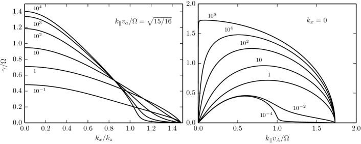
Figure 2: Dispersion relation of the MRI in the guiding center limit ($\omega_{c}/\Omega\to\infty$) for an inclined magnetic field with $b_{z}=b_{y}$. Labels give the value of $\beta_{z}=\beta/b_{z}^{2}$. These results agree well with the analogous plots shown in figs. 3 and 4 of Quataert et al. (2002).

5.3 Parallel modes ($\bm{k}\bm{\parallel}\bm{B}\bm{\parallel}\bm{\Omega}$)

In this section we study modes whose wave vector is aligned with the magnetic field, which in turn is aligned with the rotation axis. The ion response tensor in this case is given by

$$\mathbf{\Lambda}=\frac{1}{2}\sum_{\pm}\Lambda_{\pm}(\bm{e}_{1}\pm i\bm{e}_{2})(\bm{e}_{1}\mp i\bm{e}_{2})-\frac{\omega^{2}}{k_{z}^{2}v_{t}^{2}}W\left(\frac{\omega}{|k_{z}|v_{t}}\right)\bm{e}_{3}\bm{e}_{3},$$ (71)

with perpendicular components

$$\Lambda_{\pm}=\frac{\omega}{\omega\pm\omega_{g}}\left[1-W\left(\frac{\omega\pm\omega_{g}}{|k_{z}|v_{t}}\right)\right].$$ (72)

At this point we note that even in the case of a purely vertical magnetic field ($\bm{B}=B_{z}\bm{e}_{z}$), the coordinate basis $(\bm{e}_{1},\bm{e}_{2},\bm{e}_{3})$ as defined in Section 4.2 does not in general coincide with $(\bm{e}_{x},\bm{e}_{y},\bm{e}_{z})$. This is because $\bm{e}_{3}=\bm{\omega}_{g}/\omega_{g}$, and whether the gyro-frequency vector $\bm{\omega}_{g}$ is aligned or anti-aligned with the angular frequency vector $\bm{\Omega}=\Omega\bm{e}_{z}$ depends on the sign of $S_{z}=\omega_{c}{}b_{z}+2\Omega$. In this context we also note that the gyration frequency $\omega_{g}>0$ throughout this text. The cyclotron frequency $\omega_{c}=eB/m$ can have either sign, but this depends only on the sign of the charge, not on the direction of the magnetic field.

In the absence of Coriolis and tidal forces, $\Lambda_{+}$ ($\Lambda_{-}$) would describe a right (left) handed circularly polarized wave. Insertion of eq. 71 with eq. 72 into eq. 67 yields the perpendicular dispersion tensor

$$\mathbf{D}_{\perp}\doteq k_{z}^{2}v_{a}^{2}\begin{pmatrix}1&0\\ 0&1\end{pmatrix}+\omega_{c}^{2}\begin{pmatrix}1&0\\ 0&\omega_{g}/S_{z}\end{pmatrix}\cdot\begin{pmatrix}\Re&\Im\\ -\Im&\Re\end{pmatrix}\cdot\begin{pmatrix}1&0\\ 0&\omega_{g}/S_{z}\end{pmatrix}-i\omega\omega_{c}b_{z}\begin{pmatrix}0&-1\\ 1&0\end{pmatrix}-2q\Omega^{2}\frac{\omega_{c}b_{z}}{S_{z}}\begin{pmatrix}0&0\\ 0&1\end{pmatrix},$$ (73)

where the right hand side is the matrix representation of $\mathbf{D}_{\perp}$ in the basis $(\bm{e}_{x},\bm{e}_{y})$. We have also introduced the short hands

$$\Re=\frac{1}{2}(\Lambda_{+}+\Lambda_{-})\quad\textrm{and}\quad\Im=\frac{1}{2i}(\Lambda_{+}-\Lambda_{-}).$$ (74)

We note that $\Lambda_{-}=\Lambda_{+}^{\ast}$ for purely imaginary $\omega$. In this case, $\Re$ and $\Im$ are simply the real and imaginary parts of $\Lambda_{+}$.

5.3.1 Cold ions

The dispersion relation simplifies significantly in the cold ion limit $v_{t}\to 0$. In this case we may drop the $W$-function in eq. 72. The dispersion relation $\det\mathbf{D}_{\perp}=0$ may then be written as

$$\frac{k_{z}^{4}v_{a}^{4}(\omega^{2}-\omega_{g}^{2})-k_{z}^{2}v_{a}^{2}\omega_{c}b_{z}[q\Omega(\omega^{2}-\kappa^{2})-2(\omega^{2}+q\Omega^{2})\omega_{c}b_{z}]-\omega^{2}(\omega^{2}-\kappa^{2})\omega_{c}^{2}}{\omega^{2}-\omega_{g}^{2}}=0.$$ (75)

The numerator reproduces the Hall limit of the dispersion relation given by Wardle (1999). We refer the reader to that paper as well as to Balbus and Terquem (2001) for discussions of the Hall MRI. Here we only summarize several key findings.

Equation 75 is quadratic in both $\omega^{2}$ and $k^{2}$. Its discriminant with respect to $\omega^{2}$ is positive definite. Thus there are no over-stable solutions. The maximum growth rate is $\gamma=q\Omega/2$ at

$$k_{z}=\frac{\Omega}{v_{a}}\sqrt{1-\alpha^{4}}{\left[1+\frac{1}{2}(1+\alpha^{2})\frac{2\Omega}{\omega_{c}b_{z}}\right]}^{-1/2}\quad\textrm{with}\quad\alpha=\frac{\kappa}{2\Omega},$$ (76)

cf. eq. (29) of Wardle (1999). Remarkably, the maximum growth rate is independent of $\omega_{c}$. The system is thus unstable even as $\omega_{c}\to 0$. Below we will see that this is also the case if the ions are hot. This behavior might seem paradoxical in light of the result of Section 4.4.1, where we have shown that an initially unmagnetized charge-neutral cold collisionless plasma is linearly stable in the shearing sheet. The resolution of this apparent paradox is that here, it is only the ion cyclotron frequency $\omega_{c}=\omega_{ci}$ that goes to zero whereas the electron cyclotron frequency $\omega_{ce}$ is formally infinite since we have assumed the electrons to be massless. We note, however, that for realistic plasmas with finite mass ratios, it is at least questionable whether taking the limit $\omega_{ce}\to\infty$ before letting $\omega_{ci}\to{}0$ is physically meaningful.

5.3.2 Gyro-viscous correction

In Section 5.2 we have shown that we recover the kinetic MHD result obtained by Quataert et al. (2002) in the guiding center limit $\omega_{c}\to\infty$. For parallel modes it is easy to calculate the first order correction for finite cyclotron frequency. In order to do so, let us assume the ordering

$$\omega\sim k_{z}v_{a}\sim\Omega\sim\epsilon\beta\Omega\sim\epsilon^{2}\omega_{c},$$ (77)

where the ordering parameter $\epsilon\ll 1$. We thus assume that the plasma is hot but not too hot in the sense that $1\ll\beta\ll\omega_{c}/\Omega$. The perpendicular dispersion tensor to first order in $\epsilon$ is then given by

$$\mathbf{D}_{\perp}=(k_{z}^{2}v_{a}^{2}-\omega^{2})(\mathbf{1}-\bm{e}_{z}\bm{e}_{z})-i\omega\left(2\Omega-\frac{k_{z}^{2}v_{t}^{2}}{\omega_{c}b_{z}}\right)\bm{e}_{z}\times\mathbf{1}-2q\Omega^{2}\bm{e}_{y}\bm{e}_{y}.$$ (78)

Setting its determinant equal to zero yields the dispersion relation

$$\omega^{4}-\omega^{2}[\kappa^{2}+2k_{z}^{2}v_{a}^{2}\left(1-\beta\Omega/\omega_{c}b_{z}\right)]+k_{z}^{2}v_{a}^{2}(k_{z}^{2}v_{a}^{2}-2q\Omega^{2})=0.$$ (79)

The lowest order correction to the standard MHD dispersion relation is thus of order $\beta\Omega/\omega_{c}\ll{}1$. This is the magnitude of the gyro-viscous force relative to the magnetic tension force in the Braginskii equations, a fluid closure for weakly collisional plasmas that includes FLR effects. Ferraro (2007) provides a numerical analysis of the MRI with the gyro-viscous force taken into account. Our results confirm that gyro-viscosity is indeed the dominant FLR effect in a hot plasma, not the Hall effect.

Like the cold ion dispersion relation, eq. 78 is quadratic in both $\omega^{2}$ and $k^{2}$ and may be analyzed in the same way. The maximum growth rate

$$\gamma=\frac{q\Omega}{2}{\left[1+\frac{1}{2}(1-\alpha^{4})\frac{\beta\Omega}{\omega_{c}b_{z}}\right]}^{1/2}$$ (80)

occurs at

$$k_{z}=\frac{\Omega}{v_{a}}\sqrt{1-\alpha^{4}}{\left[1+\frac{1}{2}\frac{1-\alpha^{8}}{{(1+\alpha^{2})}^{2}}\frac{\beta\Omega}{\omega_{c}b_{z}}\right]}^{1/2},$$ (81)

where again $\alpha=\kappa/2\Omega$. As in the cold ion case there are no over-stable solutions.

5.3.3 Numerical solution

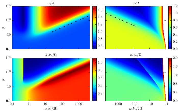
Figure 3: Growth rate and wavenumber of the fastest growing MRI mode for $\bm{k}\bm{\parallel}\bm{B}\bm{\parallel}\bm{\Omega}$ based on a numerical solution of the kinetic ion, cold, massless electron shearing sheet dispersion relation 73. The dashed black lines correspond to $\beta\Omega=\omega_{c}{}b_{z}$, the approximate ratio of the gyro-viscous force to the tension force.

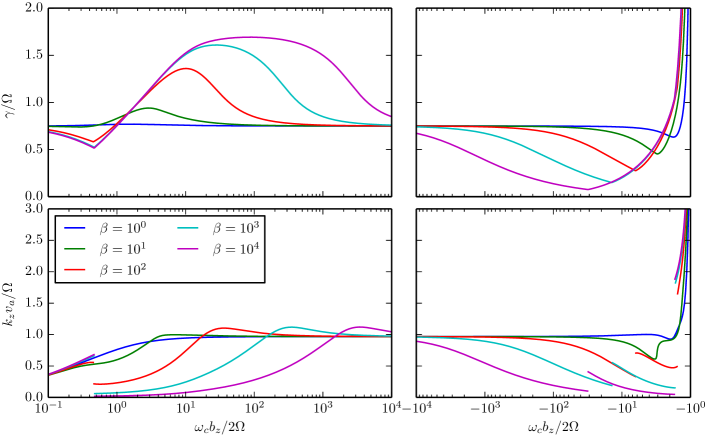
Figure 4: Growth rate and wavenumber of the fastest growing MRI mode as functions of $\omega_{c}{}b_{z}$ at fixed $\beta$. The cusps (upper panels) and discontinuities (lower panels) correspond to one local minimum of $\gamma(k_{z})$ taking over another, see fig. 5.

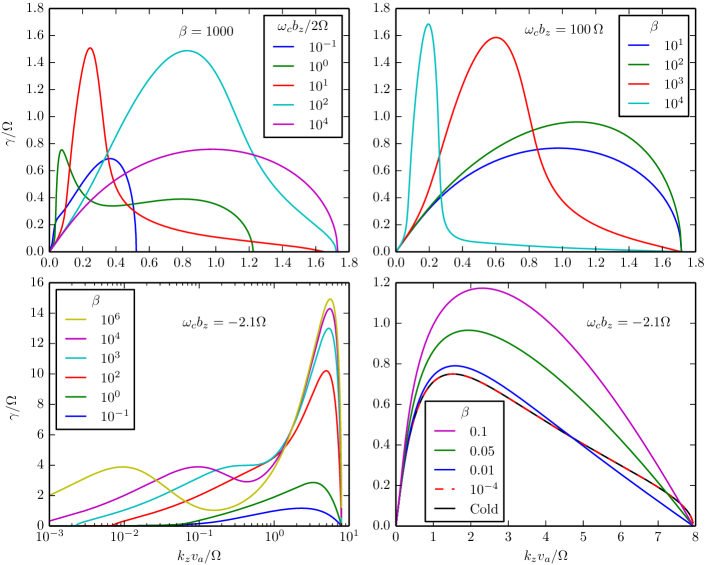
Figure 5: Plots of growth rate vs. wave number for select values of $\omega_{c}{}b_{z}$ and $\beta$. The lower panels illustrate the approach to the cold plasma dispersion relation as $\beta\to 0$ when the tidal anisotropy is large.

Outside of particular limits such as those discussed in Sections 5.3.1 and 5.3.2 the dispersion relation even for the simplest case of parallel modes with $\bm{k}\bm{\parallel}\bm{B}\bm{\parallel}\bm{\Omega}$, given in eq. 73, is transcendental in $\omega$ and $k_{z}$ and its roots can in general only be found numerically. This is the goal of this section.

Our numerical analysis has the caveat that we only look for purely growing modes. In support of this we note that the MRI is known to be purely growing in many fluid limits, including the cold ion/Hall MHD limit discussed in Section 5.3.1. In addition, the guiding center analysis carried out by Quataert et al. (2002) also yielded purely growing modes only.

For purely growing modes, the dispersion relation has a number of properties that make the root finding particularly easy. First, because the conductivity tensor vanishes as $\omega\to 0$, the dispersion relation at marginal stability is simply

$$k_{z}^{2}v_{a}^{2}\left(k_{z}^{2}v_{a}^{2}-\frac{2q\Omega^{2}\omega_{c}}{S_{z}b_{z}}\right)=0.$$ (82)

Second, the dispersion tensor is real for purely growing modes, see Section 5.3. Thus, in order to find the roots of the dispersion relation we may use Newton’s method for real valued functions. In addition, it is easy to get an overview of how many roots there are simply by plotting the dispersion relation as a function of $\gamma=\sqrt{-\omega^{2}}$. Generally we find only a single unstable root.

Equation 82 determines the range of unstable wave numbers. This range is finite provided that $\omega_{c}{}b_{z}>0$ or $\omega_{c}{}b_{z}<-2\Omega$, in which case we only need to search for roots between $k_{z}=0$ and

$$k_{z}=\frac{1}{v_{a}}\sqrt{\frac{2q\Omega^{2}\omega_{c}}{S_{z}b_{z}}}.$$ (83)

We do not consider the region of parameter space where $-2\Omega\leq\omega_{c}{}b_{z}<0$. In support of this we note that for $-2\Omega\leq\omega_{c}{}b_{z}\leq(q-2)\Omega$ the tidal anisotropy $\Delta\geq 1$, in which case the equilibrium orbits are unbound and the shearing sheet approximation rendered suspect, see the discussion in Section 3.2. For $(q-2)\Omega<\omega_{c}{}b_{z}<0$ the cold ion dispersion relation has no unstable roots (Wardle, 1999) and we were not able to find any roots (visually) for a hot plasma either.

We only consider Keplerian rotation ($q=3/2$) in our numerical solutions. The free parameters are then $\omega_{c}{}b_{z}$ and $\beta$. We sweep through this two-dimensional parameter space as follows. For each $\omega_{c}{}b_{z}$ we start with $\beta\ll 1$ and use the exact cold ion growth rate as our initial guess. We then increase $\beta$ progressively and – for each $k_{z}$ in the unstable range – use the previously obtained root as initial guess.

Figure 3 shows pseudo color plots of the maximum growth rate and associated wave number. Note that the color scales are not the same in the left and right panels, because the MRI physics depends on the sign of $b_{z}$. The black line in fig. 3 shows $\beta\Omega=\omega_{c}{}b_{z}$, suggesting that gyro-viscosity is the dominant FLR effect throughout a large portion of parameter space. Figure 4 shows cuts through fig. 3 at fixed $\beta$. The cusps in the maximum growth rate and the associated discontinuities in wave number are a consequence of the dispersion relation having more than one local maximum, as we discuss below.

Figure 4 shows that for $\omega_{c}{}b_{z}\gtrsim\Omega$ the growth rate of the fastest growing mode is always greater than the guiding center result $\gamma=q\Omega/2$. The growth rate increases with $\beta$ and appears to asymptote for a certain $\omega_{c}{}b_{z}\sim\beta\Omega$ to $\gamma=\sqrt{2q}\Omega$. This is the same as the maximum growth rate obtained by Quataert et al. (2002) and Balbus (2004) without FLR effects but with a 45^∘-inclined field; see also Section 5.2 and fig. 2. For $0<\omega_{c}{}b_{z}\lesssim\Omega$ the system is less unstable. As $\omega_{c}{}b_{z}\to 0$ from above, the maximum growth and associated wave number approach the cold ion result ($\gamma\to{}q\Omega/2$ and $k_{z}\to 0$). We note again, however, that this is a somewhat unphysical limit in which the ion cyclotron frequency goes to zero while the electron cyclotron frequency is formally infinite (recall that the latter is assumed throughout this section).

The situation is different if the field is anti-aligned with the rotation axis. For $\omega_{c}{}b_{z}\lesssim-4\Omega$ the system is always less unstable than in the guiding center limit. As $\omega_{c}{}b_{z}\to-2\Omega$ from below, however, the growth rate of the fastest growing mode as well as its wave number diverge. While this might seem odd, we note that the tidal anisotropy also diverges in this limit. This anisotropy evidently constitutes a free energy reservoir that the system is able to tap into. We also note that the diverging growth rate as $\omega_{c}{}b_{z}\to-2\Omega$ from below seems at odds with the cold ion result ($\gamma=q\Omega/2$). This is only an apparent contradiction. The growth rate does in fact approach the cold ion result for any $\omega_{c}{}b_{z}<-2\Omega$ as $\beta\to 0$.

Figure 5 show plots of $\gamma(k_{z})$ for various values of $\omega_{c}{}b_{z}$ and $\beta$. The dispersion relation can have more than one local maximum. The discontinuities visible in the maximum growth rate and associated wavenumber in figs. 3 and 4 correspond to one local maximum in fig. 5 overtaking another. The lower right panel demonstrates that for a fiducial $\omega_{c}{}b_{z}=-2.1\Omega$, the growth rate indeed approaches the cold ion result as $\beta\to 0$.

6 Conclusions

In this paper, we have studied the linear theory of a collisionless plasma in the shearing sheet approximation. This approximation isolates the key local physics of differentially rotating disks and is free from the complications of global boundary conditions. It is the ideal model for studying the local dynamics of accretion disks. Our study is motivated by the application to the magneto-rotational instability (MRI) in such disks if the accreting plasma is collisionless.

We have for the first time derived the general linear conductivity tensor for a collisionless plasma in the shearing sheet approximation. This accounts for the complete linear dynamics of kinetic ions and kinetic electrons with finite Larmor radius/cyclotron frequency. Our calculation has leveraged the extensive literature on analogous calculations for uniform plasmas (Ichimaru, 1973). In particular, we have shown that by a suitable choice of velocity space coordinates, the linear conductivity tensor for a collisionless plasma in the shearing sheet approximation can be expressed using standard results for a uniform plasma (Sections 4.1 and C). In doing so, our primary assumptions are charge-neutrality, axisymmetric perturbations, and no vertical stratification. The charge-neutral approximation is made both for its applicability to realistic accretion disk dynamics and because the shearing sheet approximation in its standard form relies on Galilean invariance, which in turn necessitates charge-neutrality once the displacement current is dropped (see e.g. Grad, 1966).

The resulting dispersion relation for a collisionless plasma in the shearing sheet approximation is given in eq. 39 with the conductivity tensor given in eq. 45. These results apply for any equilibrium distribution function. In general, the tidal force imposes a temperature anisotropy on the equilibrium distribution function, see eq. 15 and Section 3. This anisotropy vanishes only in the guiding center limit in which the ratio of the cyclotron frequency to the angular frequency $\omega_{c}/\Omega\rightarrow\infty$. We denote a “quasi-Maxwellian” distribution function with this minimal level of temperature anisotropy as the “electromagnetic Schwarzschild distribution” because it is a generalization of the Schwarzschild distribution of stellar dynamics to an ionized plasma. The conductivity tensor for this distribution function is given in equations eqs. 49, 50 and 51. These results for the linear theory of the shearing sheet are likely to be applicable to a wide range of linear stability calculations, beyond those we have carried out in this paper.

We have focused on the application of our results to the linear theory of the MRI in collisionless plasmas. In particular, we have shown that the extensive existing literature on kinetic calculations of the MRI can all be understood as approximations to the more general theory derived here. Specifically, the guiding center kinetic MRI results of Quataert et al. (2002) follow from the high cyclotron frequency and cold, massless electron limit of our dispersion relation (Section 5.2). The numerical gyro-viscous results of Ferraro (2007) – which represent finite cyclotron frequency corrections to the guiding center results of Quataert et al. (2002) – follow analytically from our dispersion relation by keeping the leading order cyclotron frequency corrections to the guiding center result (Section 5.3.2). And the Hall MHD results of Wardle (1999) – which are particularly important in the context of protostellar accretion disks – follow from the cold ion and cold, massless electron limit of our dispersion relation (Section 5.3.1).

In addition to providing a more general framework for understanding existing calculations of the MRI in kinetic theory, we have also derived a number of new results. In Sections 5.1 and D we derive the dispersion relation for the MRI in the limit of kinetic ions, but cold, massless electrons. We solve this dispersion relation for the simplest case of $\bm{k}\parallel\bm{\Omega}\parallel\bm{B}$ in Section 5.3. These numerical solutions of the full hot plasma dispersion relation confirm that the primary finite cyclotron frequency correction to the guiding-center MRI dispersion relation for $\beta\gtrsim 1$ collisionless plasmas is not the Hall effect, but rather gyro-viscosity (Ferraro, 2007).

The fluid electron, kinetic ion model of the shearing sheet studied in Sections 5.1 and D is known as the Vlasov-fluid model. It has a number of attractive features for numerical studies of the MRI in collisionless plasmas. In particular, the short length-scale, fast timescale electron dynamics is ordered out allowing one to focus computational resources on the ion dynamics that is likely the most important for the overall evolution and saturation of the MRI.

As a second application of our results, we have derived the dispersion relation of a cold plasma in the shearing sheet approximation (Section 4.4). This problem was previously studied by Krolik and Zweibel (2006), who claimed that a cold, differentially rotating plasma that is initially unmagnetized is linearly unstable to local axisymmetric perturbations. We have shown, however, that such a plasma is in fact linearly stable (Section 4.4.1).

Starting with Section 5.3, our analytical and numerical analysis of the MRI in a hot plasma has focused on “parallel modes” with $\bm{k}\parallel\bm{\Omega}\parallel\bm{B}$. In this case, the kinetic corrections to the MRI (as well any other linear waves/modes that may be present) are due to finite cyclotron frequency effects. However, the full dispersion relation derived in Section 4 also includes finite Larmor radius effects that become important when $k_{\perp}v_{t}\sim\omega_{g}$. While differential rotation is unlikely to be important on such scales if $\omega_{c}\gg\Omega$, the scale separation between $\omega_{c}$ and $\Omega$ that can be achieved in numerical simulations is always limited (unless of course the guiding center motion is averaged over, as in gyrokinetic simulations). Thus, even if the interplay between orbital motion and Larmor motion is insignificant in a given astrophysical system, our dispersion relation can be useful for benchmarking a code used to simulate said system.

Possible future applications of our analysis include studies of the stability of linear shear profiles in collisionless plasmas and the possibility of velocity space instabilities driven by the background temperature anisotropy present in differentially rotating plasmas. In addition, all existing kinetic calculations of the MRI assume cold electrons, motivated by the fact that hot accretion flows onto compact objects are believed to have $T_{i}\gtrsim{}T_{e}$. However, the general conductivity tensor given in Section 4.1 applies equally well to kinetic electrons and can be used to assess the applicability of the cold electron approximation under realistic accretion disk conditions. Finally, our calculations can be used to determine the properties of the MRI under the conditions achievable in laboratory experiments aimed at studying low collisionality high-$\beta$ plasmas (e.g. Collins et al., 2012).

Appendix A The unperturbed Hamiltonian

In this section we derive the unperturbed Hamiltonian given in eq. 9. Let us start with the Hamiltonian governing the dynamics of charged particles in a rotating frame. This is given by

$$\mathcal{H}=\frac{1}{2}{\left(\bm{p}-\bm{\Omega}\times\bm{r}-\frac{e}{m}\bm{A}\right)}^{2}+\psi+\frac{e}{m}\Phi,$$ (84)

where $\bm{A}$ is the magnetic vector potential and $\Phi$ is the electrostatic potential. The coordinate system is oriented such that $\bm{\Omega}=\Omega\bm{e}_{z}$. In the shearing sheet approximation, the tidal potential $\psi$ is given as in eq. 3 by

$$\psi=-q\Omega^{2}x^{2}+\frac{1}{2}\nu^{2}z^{2}.$$ (85)

It is straightforward to verify that $\partial{}f/\partial{}t+\{f,\mathcal{H}\}=0$ is the same as the Vlasov equation 1 when the former is expressed in terms of the particle velocity $\bm{v}=\bm{p}+\bm{\Omega}\times\bm{r}+e\bm{A}/m$.

We now consider the equilibrium discussed in Section 3, consisting of a linear shear flow and a uniform magnetic field. Without loss of generality we may (at first) work in the so-called symmetric gauge, in which the vector potential is given by $\bm{A}=\bm{B}\times\bm{r}/2$. The magnetic field is assumed frozen into the background shear flow. The corresponding electric field derives from the electrostatic potential $\Phi=-q\Omega{}xA_{y}$. With this, the Hamiltonian may be written as

$$2\mathcal{H}={\left(\bm{p}-\frac{\bm{S}\times\bm{r}}{2}\right)}^{2}-q\Omega S_{z}x^{2}+\nu^{2}x^{2}.$$ (86)

The Hamiltonian 9 is obtained after a canonical transformation to new coordinates $(\bm{r}^{\prime},\bm{p}^{\prime})$ derived from the type-2 generating function

$$G(\bm{r},\bm{p}^{\prime})=xp_{x}^{\prime}+yp_{y}^{\prime}-S_{z}xy/2.$$ (87)

Appendix B Global equilibrium

In this section we investigate the stability of charged particles on circular orbits in a global disk equilibrium. We also derive a generalization of the modified Schwarzschild distribution (Shu, 1969) and show that for nearly circular orbits it reduces to the “electromagnetic Schwarzschild distribution” used in the main text.

B.1 Bulk flow and electromagnetic field configuration

We seek an axisymmetric equilibrium with a purely rotational bulk flow common to all plasma species. In a cylindrical coordinate system $(r,\varphi,z)$, this bulk flow may be written as

$$\bm{u}=r\Omega\nabla\varphi,$$ (88)

where $\Omega(r,z)$ is the orbital frequency. Following Kaufman (1972); Cary and Littlejohn (1983) we write the magnetic field as

$$\bm{B}=\nabla w(\psi)\times\nabla\vartheta-\nabla\psi\times\nabla\varphi,$$ (89)

where $\psi(r,z)$ is the poloidal flux function. The poloidal angle $\vartheta(r,z)$ may be chosen to increase clockwise from $-\pi$ to $\pi$ along poloidal field lines, which are isocontours of $\psi$. Note that the first term on the right hand side of eq. 89 represents the toroidal field. The second term is the usual parametrization of an axisymmetric poloidal field. The magnetic field given in eq. 89 derives from the axisymmetric vector potential

$$\bm{A}=w(\psi)\nabla\vartheta-\psi\nabla\varphi.$$ (90)

The electric field is determined from the condition that the magnetic field be frozen into the equilibrium flow, to wit

$$\bm{E}=-\bm{u}\times\bm{B}.$$ (91)

This must be irrotational, thus

$$\nabla\times\bm{E}=\left(\frac{\partial\vartheta}{\partial r}\frac{\partial\psi}{\partial z}-\frac{\partial\psi}{\partial r}\frac{\partial\vartheta}{\partial z}\right)\frac{\partial\Omega}{\partial\vartheta}r\nabla\varphi=0.$$ (92)

The factor in parentheses is the Jacobian of the transformation from flux coordinates $(\psi,\varphi,\vartheta)$ to cylindrical coordinates $(r,\varphi,z)$. Assuming this is non-singular, it follows that the orbital frequency $\Omega(\psi)$ is constant on poloidal field lines (Ferraro, 1937), see also Papaloizou and Szuszkiewicz (1992). With this result, it easy to show that the electric field derives from the electrostatic potential

$$\Phi(\psi)=-\int\!\Omega(\psi)\,d\psi.$$ (93)

B.2 Stability of circular orbits

The equations of motion for charged particles orbiting in the equilibrium fields are generated by the Hamiltonian

$$\mathcal{H}=\frac{1}{2}\left[{\left(p_{r}-\frac{e}{m}A_{r}\right)}^{2}+\frac{1}{r^{2}}{\left(p_{\varphi}+\frac{e}{m}\psi\right)}^{2}+{\left(p_{z}-\frac{e}{m}A_{z}\right)}^{2}\right]+\Psi+\frac{e}{m}\Phi,$$ (94)

where $\Psi(r,z)$ is the gravitational potential. The equilibrium Hamiltonian is independent of $\varphi$ due to the assumed axial symmetry. The canonical angular momentum

$$p_{\varphi}=r^{2}\dot{\varphi}-\frac{e}{m}\psi$$ (95)

is thus an integral of motion and for a given $p_{\varphi}$, the dynamics may be described in the reduced phase space $(r,z,p_{r},p_{z})$.

We assume that the equilibrium also has equatorial symmetry. By this we mean that there is a plane of symmetry at $z=0$ (the mid-plane) and that the equilibrium fields are either even or odd functions of $z$. Specifically, we take the gravitational and electrostatic potentials as well as the poloidal flux $\psi$ to be even, and the poloidal angle $\vartheta$ to be odd. This completely specifies the equatorial symmetry of the equilibrium.

Using Hamilton’s equation, the first variation of eq. 94 is $\delta\mathcal{H}=\dot{r}\delta{}p_{r}+\dot{z}\delta{}p_{z}-\dot{p}_{r}\delta{}r-\dot{p}_{z}\delta{}z$. All equilibrium points in phase space (for which $\delta\mathcal{H}=0$) are thus circular orbits ($\dot{r}=\dot{z}=0$). For such orbits, the rates of change of the canonical momenta are

$$\dot{p}_{r} =\frac{e}{m}r(\dot{\varphi}-\Omega)B_{z}-\frac{\partial\Psi}{\partial r}+r\dot{\varphi}^{2}$$ (96)

$$\dot{p}_{z} =\frac{e}{m}r(\Omega-\dot{\varphi})B_{r}-\frac{\partial\Psi}{\partial z},$$ (97)

where we have made use of our assumption that the electric field is frozen into the bulk flow $\bm{u}=r^{2}\Omega\nabla\varphi$. Given the equatorial symmetry of $\Psi$, particles on circular orbits are (relative) equilibria if they travel in the mid-plane ($z=0$) and their angular velocity matches that of the bulk flow, i.e. if

$$\dot{\varphi}=\Omega(r,0),$$ (98)

provided the latter arises due to gravito-centrifugal balance, i.e. provided that

$$r\Omega^{2}(r,0)=\frac{\partial\Psi(r,0)}{\partial r}.$$ (99)

From now on it will be understood that all quantities are evaluated at $z=0$.

In order to determine the stability of circular orbits we can invoke the so-called Lagrange-Dirichlet theorem (see e.g. Krechetnikov and Marsden, 2007, and references therein). This states that an equilibrium point (in this case the circular orbit) is stable to finite perturbations (nonlinear stability) if the second variation of $\mathcal{H}$ (a quadratic form) or, equivalently, its Hessian is positive definite. In the phase space coordinate system $(r,z,p_{r},p_{z})$, the Hessian has the matrix representation

$$\mathbf{D}\doteq\begin{bmatrix}\displaystyle S_{z}\left(S_{z}+r\frac{\partial\Omega}{\partial r}\right)+{\left(\frac{e}{m}\frac{\partial A_{z}}{\partial r}\right)}^{2}&0&0&\displaystyle-\frac{e}{m}\frac{\partial A_{z}}{\partial r}\\ 0&\displaystyle\frac{\partial^{2}\Psi}{\partial z^{2}}+{\left(\frac{e}{m}\frac{\partial A_{r}}{\partial z}\right)}^{2}&\displaystyle-\frac{e}{m}\frac{\partial A_{r}}{\partial z}&0\\ 0&\displaystyle-\frac{e}{m}\frac{\partial A_{r}}{\partial z}&1&0\\ \displaystyle-\frac{e}{m}\frac{\partial A_{z}}{\partial r}&0&0&1\end{bmatrix},$$ (100)

where

$$\bm{S}=\frac{e}{m}\bm{B}+2\bm{\Omega}$$ (101)

is defined in the same way as in the main text, see eq. 8. The Hessian matrix given in eq. 100 is positive definite if and only if

$$S_{z}\left(S_{z}+r\frac{\partial\Omega}{\partial r}\right)>0\quad\textrm{and}\quad\frac{\partial^{2}\Psi}{\partial z^{2}}>0.$$ (102)

Otherwise the Hessian is indefinite. If the above inequalities are satisfied, then circular orbits minimize the energy. Note that if we define

$$\Delta=-\frac{r}{S_{z}}\frac{\partial\Omega}{\partial r},$$ (103)

in complete analogy to eq. 15, then the first inequality in eq. 102 is equivalent to $\Delta<1$. Note also that for circular orbits, the radial derivative of the canonical angular momentum is given by

$$\frac{\partial p_{\varphi}}{\partial r}=r\left(S_{z}+r\frac{\partial\Omega}{\partial r}\right)=rS_{z}(1-\Delta).$$ (104)

For neutral particles, the condition for stability $\Delta<1$ reduces to the familiar Rayleigh criterion

$$\kappa^{2}=2\Omega\left(2\Omega+r\frac{\partial\Omega}{\partial r}\right)>0.$$ (105)

From eq. 104 we recover the familiar result (e.g. Chandrasekhar, 1961) that the angular momentum is a decreasing function of radius in this case. For charged particles, the (canonical) angular momentum in a stable configuration does not necessarily decrease with radius because $S_{z}$ is not sign definite.

B.2.1 Linear stability

Above we have shown that circular orbits are nonlinearly stable provided that $\Delta<1$ and $\partial^{2}\Psi/\partial{}z^{2}>0$. This does not necessarily imply that circular orbits are unstable if $\Delta>1$. To see this, we consider the linearized Hamiltonian system

$$\delta\dot{\bm{w}}=\mathbf{J}\cdot\mathbf{D}\cdot\delta\bm{w},$$ (106)

where $\bm{w}=(r,z,p_{r},p_{z})$,

$$\mathbf{J}=\begin{bmatrix}0&0&1&0\\ 0&0&0&1\\ -1&0&0&0\\ 0&-1&0&0\end{bmatrix},$$ (107)

and $\mathbf{D}$ is the Hessian given in eq. 100. Assuming that $\delta\bm{w}$ depends on time as $\exp(-i\omega{}t)$, the linearized system has non-trivial solutions provided that

$$\det(i\omega\mathbf{1}+\mathbf{J}\cdot\mathbf{D})=\omega^{4}-\omega^{2}\left[S_{z}\left(S_{z}+r\frac{\partial\Omega}{\partial r}\right)+S_{\varphi}^{2}+\frac{\partial^{2}\Psi}{\partial z^{2}}\right]+S_{z}\left(S_{z}+r\frac{\partial\Omega}{\partial r}\right)\frac{\partial^{2}\Psi}{\partial z^{2}}=0,$$ (108)

where $\mathbf{1}$ denotes the identity matrix.

Let us first consider the case of a vanishing toroidal magnetic field. For $S_{\varphi}=eB_{\varphi}/m=0$, the solubility condition 108 dramatically simplifies because the radial and vertical degrees of freedom decouple. The stability of the respective motions is determined by

$$\omega^{2}=S_{z}\left(S_{z}+r\frac{\partial\Omega}{\partial r}\right)\quad\textrm{and}\quad\omega^{2}=\frac{\partial^{2}\Psi}{\partial z^{2}}.$$ (109)

Comparison with eq. 102 shows that circular orbits are linearly stable if they are nonlinearly stable (i.e. if the minimize the energy), and linearly unstable otherwise.

The situation is more complicated if there is a toroidal magnetic field. In this case there is a region of parameter space where circular orbits are linearly stable even though they do not minimize the energy. To see this, let us assume (as in the bulk of the main text) that there is no stratification ($\Psi=\mathrm{const}$). In this case, the solubility condition eq. 108 reduces to

$$\omega^{2}(\omega^{2}-\omega_{g}^{2})=0,$$ (110)

where the square of the gyration frequency $\omega_{g}$ is given by

$$\omega_{g}^{2}=S_{z}\left(S_{z}+r\frac{\partial\Omega}{\partial r}\right)+S_{\varphi}^{2}.$$ (111)

This is the global analogue of the local gyration frequency defined in eq. 22 in the main text. Equation 110 with eq. 111 implies that circular orbits are linearly stable provided that

$$\Delta<1+S_{\varphi}^{2}/S_{z}^{2},$$ (112)

which does not coincide with the nonlinear stability boundary $\Delta<1$. In this context we remark that according to a theorem due to Bloch et al. (1994), a relative equilibrium that is linearly but not nonlinearly stable becomes linearly unstable when a small amount of dissipation is added to the system. We are thus led to conclude that circular orbits in realistic systems are always unstable if $\Delta>1$, regardless of whether or not there is a toroidal magnetic field.

B.3 The modified electromagnetic Schwarzschild distribution

The electromagnetic Schwarzschild distribution 23 may be viewed as a generalization of the Schwarzschild distribution (e.g. Julian and Toomre, 1966). The latter is the local limit (nearly circular orbits) of the modified Schwarzschild distribution as derived by Shu (1969). Here we generalize the modified Schwarzschild distribution and show that it reduces to eq. 23 in the local limit.

The integrals of motion are the particle energy

$$\mathcal{E}=\frac{\dot{r}^{2}+r^{2}\dot{\varphi}^{2}+\dot{z}^{2}}{2}+\Psi+\frac{e}{m}\Phi$$ (113)

and the canonical angular momentum $p_{\varphi}$ defined in eq. 95. By Jeans’ theorem, any distribution function of the form $f(\mathcal{E},p_{\varphi})$ is a solution of the steady state Vlasov equation. Let us define the guiding center radius $r_{c}$ through

$$p_{\varphi}=r_{c}^{2}\Omega(r_{c},0)-\frac{e}{m}\psi(r_{c},0).$$ (114)

Thus, $r_{c}$ is the radius of circular orbit with angular momentum $p_{\varphi}$. Its energy is

$$\mathcal{E}_{c}=\frac{r_{c}^{2}\Omega^{2}(r_{c},0)}{2}+\Psi(r_{c},0)+\frac{e}{m}\Phi(r_{c},0).$$ (115)

Note that $\mathcal{E}_{c}$ depends only on the angular momentum and is thus an integral of motion. We define the modified electromagnetic Schwarzschild distribution as

$$f\propto\exp(-\mathcal{K}/T),$$ (116)

where

$$\mathcal{K}=\mathcal{E}-\mathcal{E}_{c}$$ (117)

is the gyration energy. The proportionality constant in eq. 116 and the temperature $T$ may in general depend on the canonical angular momentum.

We now show that for nearly circular orbits, eq. 116 reduces to the electromagnetic Schwarzschild distribution given in eq. 23. Let us first introduce the peculiar velocity

$$\tilde{\bm{v}}=\dot{\bm{r}}-r\Omega(r,z)\bm{e}_{\varphi}.$$ (118)

Substituting

$$r\dot{\varphi}=\frac{1}{r}\left[p_{\varphi}+\frac{e}{m}\psi(r,z)\right]=\frac{1}{r}\left[r_{c}^{2}\Omega(r_{c},0)+\frac{e}{m}\psi(r,z)-\frac{e}{m}\psi(r_{c},0)\right]$$ (119)

and expanding for small $\tilde{v}_{\varphi}/r\Omega$, the azimuthal component of the peculiar velocity is approximately given by

$$\tilde{v}_{\varphi}=\left[S_{z}(r,0)+r\frac{\partial\Omega(r,0)}{\partial r}\right](r-r_{c}),$$ (120)

where $\bm{S}$ is defined in eq. 101. Corrections to eq. 120 are quadratic in $r-r_{c}$ and $z$. Expanding the gyration energy defined in eq. 117 to quadratic order in $\tilde{v}_{\varphi}/r\Omega$ yields

$$2\mathcal{K}=\tilde{v}_{r}^{2}+S_{z}(r,0)\left[S_{z}(r,0)+r\frac{\partial\Omega(r,0)}{\partial r}\right]{(r-r_{c})}^{2}+\tilde{v}_{z}+\nu^{2}z^{2},$$ (121)

Here, the square of the vertical frequency $\nu$ is defined as

$$\nu^{2}=\frac{\partial^{2}\Psi}{\partial z^{2}}$$ (122)

evaluated at $z=0$. Combining eq. 120 into eq. 121 finally yields

$$\mathcal{K}=\frac{1}{2}\left[\tilde{v}_{r}^{2}+\frac{\tilde{v}_{\varphi}^{2}}{1-\Delta}+\tilde{v}_{z}^{2}\right]+\frac{\nu^{2}z^{2}}{2},$$ (123)

which is just the electromagnetic Schwarzschild distribution defined in eq. 14.

Appendix C The conductivity tensor

Here we fill in some of the details of going from the formal solution to the linearized Vlasov equation, eq. 31, to the “conductive” relationship between current and electric field, eq. 34. Note that we are assuming axisymmetric perturbations, so $k_{y}=0$.

Using Faraday’s law in the form of eq. 32, the formal solution is given by

$$\delta f_{s}=-\frac{1}{i\omega}\frac{e_{s}}{m_{s}}\int_{-\infty}^{t}\!dt^{\prime}\,\frac{\partial f_{s}}{\partial\tilde{\bm{v}}^{\prime}}\cdot[i(\omega-\bm{k}\cdot\tilde{\bm{v}}^{\prime})\mathbf{1}+i\bm{k}\tilde{\bm{v}}^{\prime}+q\Omega\bm{e}_{x}\bm{e}_{y}]\cdot\delta\tilde{\bm{E}},$$ (124)

where $\bm{r}^{\prime}(t^{\prime})$ and $\tilde{\bm{v}}^{\prime}(t^{\prime})$ satisfy $d\bm{r}^{\prime}/dt^{\prime}=\tilde{\bm{v}}^{\prime}-q\Omega{}x^{\prime}\bm{e}_{y}$ and

$$\frac{d\tilde{\bm{v}}^{\prime}}{dt^{\prime}}=\frac{e_{s}}{m_{s}}\tilde{\bm{v}}^{\prime}\times\bm{B}-2\bm{\Omega}\times\tilde{\bm{v}}^{\prime}+q\Omega\tilde{v}_{x}^{\prime}\bm{e}_{y}$$ (125)

subject to the “final conditions” $\bm{r}^{\prime}(t)=\bm{r}$ and $\tilde{\bm{v}}^{\prime}(t)=\tilde{\bm{v}}$. Taking the first moment of eq. 124, multiplying by $e_{s}n_{s}$, and summing over species yields the perturbed current density

$$\delta\bm{J}=\tilde{\bm{\sigma}}\cdot\left(\mathbf{1}-\frac{q\Omega}{i\omega}\bm{e}_{x}\bm{e}_{y}\right)\cdot\delta\tilde{\bm{E}}.$$ (126)

Here, we have introduced the tensor

$$\tilde{\bm{\sigma}}=-\frac{1}{i\omega}\sum_{s}\frac{e_{s}^{2}n_{s}}{m_{s}}\int d^{3}v\int_{0}^{\infty}d\tau\,\tilde{\bm{v}}\frac{\partial f_{s}}{\partial\tilde{\bm{v}}^{\prime}}\cdot[i(\omega-\bm{k}\cdot\tilde{\bm{v}}^{\prime})\mathbf{1}+i\bm{k}\tilde{\bm{v}}^{\prime}+q\Omega\bm{e}_{x}\bm{e}_{y}]\exp\{-i\phi(\tau)\},$$ (127)

where the new time variable $\tau=t-t^{\prime}$ and the short hand

$$\phi(\tau)=\bm{k}\cdot(\bm{r}-\bm{r}^{\prime})-\omega\tau.$$ (128)

From now on we will suppress the species index when there is no risk of confusion. In order to express eq. 127 in terms of the “gyrotropic velocity” $\bm{\mathring{v}}=\mathbf{Q}^{-1}\cdot\bm{v}$, let us first note that

$$\frac{\partial f}{\partial\tilde{\bm{v}}}=\frac{\partial f}{\partial\bm{\mathring{v}}}\cdot\mathbf{Q}+\Delta\frac{\partial f}{\partial\tilde{v}_{y}}\bm{e}_{y},$$ (129)

where the anisotropy tensor $\mathbf{Q}$ is defined in eq. 36. With this, the orbit integral in eq. 127 may be rewritten as

$$\int_{0}^{\infty}d\tau\,\frac{\partial f}{\partial\tilde{\bm{v}}^{\prime}}\cdot[i(\omega-\bm{k}\cdot\tilde{\bm{v}}^{\prime})\mathbf{1}+i\bm{k}\tilde{\bm{v}}^{\prime}+q\Omega\bm{e}_{x}\bm{e}_{y}]\,\exp\{-i\phi(\tau)\}\\ =-\Delta\frac{\partial f}{\partial\tilde{v}_{y}}\bm{e}_{y}+\int_{0}^{\infty}d\tau\,\frac{\partial f}{\partial\bm{\mathring{v}}^{\prime}}\cdot[i(\omega-\bm{k}\cdot\bm{\mathring{v}}^{\prime})\mathbf{1}+i\bm{k}\bm{\mathring{v}}^{\prime}]\cdot\mathbf{Q}\exp\{-i\phi(\tau)\}.$$ (130)

In obtaining this result we have used that

$$q\Omega\frac{\partial f}{\partial\tilde{v}_{x}^{\prime}}-\Delta\frac{\partial}{\partial\tau}\frac{\partial f}{\partial\tilde{v}_{y}^{\prime}}=\left(q\Omega\tilde{v}_{x}^{\prime}-\frac{\Delta}{1-\Delta}\frac{\partial\tilde{v}_{y}^{\prime}}{\partial\tau}\right)\frac{1}{\mathring{v}_{\perp}}\frac{\partial f}{\partial\mathring{v}_{\perp}}=0.$$ (131)

The second equality in follows from eq. 125. To get the first equality, notice that

$$\frac{\partial f}{\partial\tilde{v}_{x}}=\frac{\tilde{v}_{x}}{\mathring{v}_{\perp}}\frac{\partial f}{\partial\mathring{v}_{\perp}}\quad\textrm{and}\quad\frac{\partial f}{\partial\tilde{v}_{y}}=\frac{1}{1-\Delta}\frac{\tilde{v}_{y}}{\mathring{v}_{\perp}}\frac{\partial f}{\partial\mathring{v}_{\perp}}+\frac{\mathring{v}_{\parallel}\sin\varphi}{\sqrt{1-\Delta}}\left(\frac{1}{\mathring{v}_{\perp}}\frac{\partial f}{\partial\mathring{v}_{\perp}}-\frac{1}{\mathring{v}_{\parallel}}\frac{\partial f}{\partial\mathring{v}_{\parallel}}\right),$$ (132)

where $\varphi$ is defined through $\bm{\omega}_{g}=\bm{e}_{z}\cos\varphi-\bm{e}_{y}\sin\varphi$. The second term in the expression for $\partial{}f/\partial\tilde{v}_{y}$ does not depend on time and therefore makes no contribution in eq. 131. Using eq. 130 in eq. 127 and integrating the contribution from the first term on the right hand side of eq. 130 by parts yields

$$\tilde{\bm{\sigma}}=\bm{\sigma}-\frac{1}{i\omega}\sum_{s}\frac{e_{s}^{2}n_{s}}{m_{s}}\Delta_{s}\bm{e}_{y}\bm{e}_{y}$$ (133)

with the conductivity tensor $\bm{\sigma}$ as defined in eq. 37. Inserting eq. 133 into eq. 126 then finally yields eq. 34.

Appendix D Vlasov-fluid dispersion relation

The Vlasov-fluid equations (Freidberg, 1972) describe the low-frequency electromagnetic interaction of collisionless ions with a massless and isotropic electron fluid. A detailed description is given in the recent work by Cerfon and Freidberg (2011). Here we show explicitly that the Vlasov fluid dispersion relation in the shearing sheet is equivalent to the cold, massless electron limit of the general hot plasma shearing sheet dispersion relation derived in Section 5.1 (up to a term related to electron pressure that is included in the Vlasov fluid model as a crude representation of finite electron temperature effects). The Vlasov fluid calculation presented here is useful primarily in that it provides an independent formalism for calculating the shearing sheet dispersion relation in the limit in which ion dynamics are the most important. In addition, the Vlasov fluid derivation is somewhat more similar to the MHD calculation in that it utilizes the Lagrangian displacement and the fact that field lines are frozen into the electron fluid.

D.1 The Vlasov-fluid equations

The electrons dynamics are described by the momentum equation

$$en_{e}(\bm{E}+\bm{u}_{e}\times\bm{B})+\nabla p_{e}=0,$$ (134)

which we will henceforth refer to as the generalized Ohm’s law. Here, we assume that the electron pressure $p_{e}$ is a function of the electron number density $n_{e}$ alone, i.e. we assume a barotropic equation of state. Equation 134 arises out of the electron momentum equation in the limit of vanishing electron mass and assuming an isotropic pressure. The electrons must be collisional for this assumption to be reasonable. Indeed, Rosin et al. (2011) derive eq. 134 rigorously through an expansion in the electron-to-ion mass ratio under the assumption of weakly collisional ions but strongly collisional electrons.

The crude electron model represents the most severe limitation of Vlasov-fluid theory. At the same time it may, however, also be viewed as the theory’s greatest merit. This is because the fast electron scales are not part of the problem anymore: The plasma frequency and Debye length are not finite due to charge-neutrality and neither is the electron Larmor motion due to the vanishing electron mass. The absence of these fast time scales simplifies the analysis and significantly reduces the computational burden in numerical simulations (Byers et al., 1978; Winske et al., 2003; Kunz et al., 2014).

The electromagnetic field is described by the pre-Maxwell equations. Ampère’s law $\mu_{0}\bm{J}=\nabla\times\bm{B}$ thus lacks the displacement current. The system of equations is closed with the definition of the current density

$$\bm{J}=-en_{e}\bm{u}_{e}+\sum_{s}e_{s}\int d^{3}v\,\bm{v}f_{s}$$ (135)

and the charge-neutrality condition

$$en_{e}=\sum_{s}e_{s}\int d^{3}v\,f_{s},$$ (136)

where the summation is over ion species only.

The electron velocity $\bm{u}_{e}$ plays a more fundamental role in Vlasov-fluid theory than may be apparent at first sight. Differentiating eq. 136 with respect to time yields after a little bit of algebra the continuity equation

$$\frac{\partial n_{e}}{\partial t}+\nabla\cdot(n_{e}\bm{u}_{e})=0.$$ (137)

With the barotropic assumption, eliminating the electric field between Ohm’s law and Faraday’s law yields the induction equation

$$\frac{\partial\bm{B}}{\partial t}=\nabla\times(\bm{u}_{e}\times\bm{B}).$$ (138)

The magnetic field is thus frozen into the electron fluid. The form of eqs. 137 and 138 suggests that in linear theory we introduce the Lagrangian displacement through

$$\delta\bm{u}_{e}+\bm{\xi}\cdot\nabla\bm{u}_{e}=\left(\frac{\partial}{\partial t}+\bm{u}_{e}\cdot\nabla\right)\bm{\xi}$$ (139)

cf. Lynden-Bell and Ostriker (1967); Friedman and Schutz (1978). The linearized eqs. 137 and 138 are then easily integrated to yield

$$\delta n_{e}+\nabla\cdot(n_{e}\bm{\xi})=0$$ (140)

and

$$\delta\bm{B}=\nabla\times(\bm{\xi}\times\bm{B}).$$ (141)

We stress that eqs. 139, 140 and 141 hold for general equilibria.

D.2 The dispersion relation in the shearing sheet

In this section we linearize the Vlasov-fluid equations around the equilibrium discussed in Section 3. The equilibrium bulk velocity common to all species is thus given by the linear shear flow 5. As in Section 4.1 we will work in terms of the invariant velocity $\tilde{\bm{v}}$ and electric field $\tilde{\bm{E}}$ as defined in eq. 27. We thus use the Vlasov equation and Faraday’s law in the form of eqs. 28 and 29, respectively. Also introducing the invariant electron velocity

$$\tilde{\bm{u}}_{e}=\bm{u}_{e}+q\Omega x\bm{e}_{y},$$ (142)

the generalized Ohm’s law reads

$$en_{e}(\tilde{\bm{E}}+\tilde{\bm{u}}_{e}\times\bm{B})+\nabla p_{e}=0,$$ (143)

and the electric current density is given by

$$\bm{J}=-en_{e}\tilde{\bm{u}}_{e}+\sum_{s}e_{s}\int d^{3}v\,\tilde{\bm{v}}f_{s}.$$ (144)

The dispersion relation is obtained by linearizing eq. 144 and expressing it entirely in terms of the Lagrangian displacement $\bm{\xi}$. As in Section 4.1 we consider an axisymmetric plane wave. Equation 139 then reduces to

$$\delta\tilde{\bm{u}}_{e}=-i\omega\bm{\xi}+q\Omega\xi_{x}\bm{e}_{y}.$$ (145)

The ion current is given by the right hand side of eq. 34, to wit

$$\sum_{s}e_{s}\int d^{3}v\,\tilde{\bm{v}}\,\delta f_{s}=\left(\bm{\sigma}-\frac{1}{i\omega}\sum_{s}\frac{e_{s}^{2}n_{s}}{m_{s}}\Delta_{s}\bm{e}_{y}\bm{e}_{y}\right)\cdot\left(\mathbf{1}-\frac{q\Omega}{i\omega}\bm{e}_{x}\bm{e}_{y}\right)\cdot\delta\tilde{\bm{E}},$$ (146)

where the ion conductivity tensor $\bm{\sigma}$ is defined in eq. 37 with the understanding that the summation in this case is over ion species only. The electric field is obtained from the generalized Ohm’s law in the form of eq. 143. Using eqs. 145 and 141 to eliminate the electron density and velocity yields

$$\delta\tilde{\bm{E}}=(i\omega\mathbf{1}+q\Omega\bm{e}_{x}\bm{e}_{y})\cdot(\bm{\xi}\times\bm{B})+e^{-1}dp_{e}/dn_{e}\nabla\nabla\cdot\bm{\xi}.$$ (147)

Finally, we combine Ampère’s law and eq. 141 to obtain

$$\mu_{0}\delta\bm{J}=\nabla\times[\nabla\times(\bm{\xi}\times\bm{B})].$$ (148)

Putting everything together yields after some algebra

$$\mu_{0}^{-1}\nabla\times\nabla\times(\bm{\xi}\times\bm{B})=en_{e}i\omega\bm{\xi}+\bm{\sigma}\cdot(i\omega\bm{\xi}\times\bm{B}+e^{-1}dp_{e}/dn_{e}\nabla\nabla\cdot\bm{\xi})-2q\Omega^{2}\xi_{x}\bm{e}_{y}\sum_{s}\frac{e_{s}n_{s}}{\omega_{cs}b_{z}+2\Omega}.$$ (149)

Assuming a plane wave decomposition, this equation may be written as $\mathbf{D}\cdot\bm{\xi}=0$ with the dispersion tensor given by

$$\mathbf{D}=\left[(k^{2}\mathbf{1}-\bm{k}\bm{k}-i\omega\mu_{0}\bm{\sigma})v_{a}^{2}-i\omega\bar{\omega}_{c}\bm{b}\times\mathbf{1}-2q\Omega^{2}\sum_{s}\frac{n_{s}m_{s}}{\rho}\frac{\omega_{cs}/b_{z}}{\omega_{cs}b_{z}+2\Omega}\bm{e}_{y}\bm{e}_{y}\right]\times\bm{b}+\bar{\omega}_{c}\left(i\omega\bm{b}\bm{b}-\frac{\bm{\sigma}\cdot\bm{k}\bm{k}}{e^{2}n_{e}}\frac{dp_{e}}{dn_{e}}\right),$$ (150)

where

$$\bar{\omega}_{c}=\frac{en_{e}B}{\rho}=\sum_{s}\frac{n_{s}m_{s}}{\rho}\,\omega_{cs}$$ (151)

is the mass-weighted mean cyclotron frequency. The perpendicular components of eq. 150 agree with eq. 65.

References

- Hill (1878) G. W. Hill, American Journal of Mathematics 1, 129 (1878).
- Goldreich and Lynden-Bell (1965) P. Goldreich and D. Lynden-Bell, Monthly Notices of the Royal Astronomical Society 130, 125 (1965).
- Hawley et al. (1996) J. F. Hawley, C. F. Gammie, and S. A. Balbus, The Astrophysical Journal 464, 690 (1996).
- Rees et al. (1982) M. J. Rees, M. C. Begelman, R. D. Blandford, and E. S. Phinney, Nature 295, 17 (1982).
- Yuan and Narayan (2012) F. Yuan and R. Narayan, Annual Review of Astronomy and Astrophysics 52 (2012).
- Julian and Toomre (1966) W. H. Julian and A. Toomre, The Astrophysical Journal 146, 810 (1966).
- Ichimaru (1973) S. Ichimaru, Basic principles of plasma physics: a statistical approach (Benjamin/Cummings Publishing Company, 1973).
- Krall and Trivelpiece (1973) N. A. Krall and A. W. Trivelpiece, Principles of plasma physics (McGraw-Hill, New York, 1973).
- Stix (1992) T. H. Stix, Waves in Plasmas (American Institute of Physics, New York, 1992).
- Quataert et al. (2002) E. Quataert, W. Dorland, and G. W. Hammett, The Astrophysical Journal 577, 524 (2002).
- Wardle (1999) M. Wardle, Monthly Notices of the Royal Astronomical Society 307, 849 (1999).
- Ferraro (2007) N. M. Ferraro, The Astrophysical Journal 662, 512 (2007).
- Krolik and Zweibel (2006) J. H. Krolik and E. G. Zweibel, The Astrophysical Journal 644, 651 (2006).
- Wisdom and Tremaine (1988) J. Wisdom and S. Tremaine, The Astronomical Journal 95, 925 (1988).
- Ferraro (1937) V. C. A. Ferraro, Monthly Notices of the Royal Astronomical Society 97, 458 (1937).
- Shu (1969) F. H. Shu, The Astrophysical Journal 158, 505 (1969).
- Kaufman (1971) A. N. Kaufman, Physics of Fluids 14, 387 (1971).
- Kaufman (1972) A. N. Kaufman, Physics of Fluids 15, 1063 (1972).
- Thomson (1887) W. Thomson, Philosophical Magazine Series 5 24, 188 (1887).
- Lees and Edwards (1972) A. W. Lees and S. F. Edwards, Journal of Physics C: Solid State Physics 5, 1921 (1972).
- Hawley et al. (1995) J. F. Hawley, C. F. Gammie, and S. A. Balbus, The Astrophysical Journal 440, 742 (1995).
- Fried and Conte (1961) B. D. Fried and S. D. Conte, The Plasma Dispersion Function (Academic Press, New York, 1961).
- Balbus and Terquem (2001) S. A. Balbus and C. Terquem, The Astrophysical Journal 552, 235 (2001).
- Grad (1961) H. Grad, Microscopic and Macroscopic Models in Plasma Physics, Tech. Rep. (1961).
- Freidberg (1972) J. P. Freidberg, Physics of Fluids 15, 1102 (1972).
- Kulsrud (1983) R. M. Kulsrud, in Handbook of Plasma Physics, Vol. 1, edited by M. N. Rosenbluth and R. Sagdeev (North Holland, New York, 1983) Chap. 1.4, pp. 115–145.
- Hazeltine and Waelbroeck (2004) R. D. Hazeltine and F. L. Waelbroeck, The Framework of Plasma Physics (Westview, Boulder, CO, 2004).
- Balbus (2004) S. A. Balbus, The Astrophysical Journal 616, 857 (2004).
- Schekochihin et al. (2005) A. A. Schekochihin, S. C. Cowley, R. M. Kulsrud, G. W. Hammett, and P. Sharma, The Astrophysical Journal 629, 139 (2005).
- Sharma et al. (2006) P. Sharma, G. W. Hammett, E. Quataert, and J. M. Stone, The Astrophysical Journal 637, 952 (2006).
- Grad (1966) H. Grad, The Guiding Center Plasma, Tech. Rep. (1966).
- Collins et al. (2012) C. Collins, N. Katz, J. Wallace, J. Jara-Almonte, I. Reese, E. Zweibel, and C. B. Forest, Physical Review Letters 108, 115001 (2012).
- Cary and Littlejohn (1983) J. R. Cary and R. G. Littlejohn, Annals of Physics 151, 1 (1983).
- Papaloizou and Szuszkiewicz (1992) J. C. B. Papaloizou and E. Szuszkiewicz, Geophysical & Astrophysical Fluid Dynamics 66, 223 (1992).
- Krechetnikov and Marsden (2007) R. Krechetnikov and J. E. Marsden, Reviews of Modern Physics 79, 519 (2007).
- Chandrasekhar (1961) S. Chandrasekhar, International Series of Monographs on Physics, Oxford: Clarendon, 1961 (Dover Publications, Oxford, 1961).
- Holm et al. (1985) D. D. Holm, J. E. Marsden, T. Ratiu, and A. Weinstein, Physics Reports 123, 1 (1985).
- Bloch et al. (1994) A. Bloch, P. S. Krishnaprasad, J. E. Marsden, and T. Ratiu, Annales de l’Institut Henri Poincaré (C) Analyse Non Linéaire 11, 37 (1994).
- Cerfon and Freidberg (2011) A. J. Cerfon and J. P. Freidberg, Physics of Plasmas 18, 012505 (2011).
- Rosin et al. (2011) M. S. Rosin, A. A. Schekochihin, F. Rincon, and S. C. Cowley, Monthly Notices of the Royal Astronomical Society 413, 7 (2011).
- Byers et al. (1978) J. A. Byers, B. I. Cohen, W. C. Condit, and J. D. Hanson, Journal of Computational Physics 27, 363 (1978).
- Winske et al. (2003) D. Winske, L. Yin, N. Omidi, H. Karimabadi, and K. Quest, in Lecture Notes in Physics: Space Plasma Simulation, edited by J. Büchner, M. Scholer, and C. Dum (Springer Berlin/Heidelberg, 2003) pp. 136–165.
- Kunz et al. (2014) M. W. Kunz, J. M. Stone, and X.-N. Bai, Journal of Computational Physics 259, 154 (2014).
- Lynden-Bell and Ostriker (1967) D. Lynden-Bell and J. P. Ostriker, Monthly Notices of the Royal Astronomical Society 136, 293 (1967).
- Friedman and Schutz (1978) J. L. Friedman and B. F. Schutz, The Astrophysical Journal 221, 937 (1978).