McGehee regularization of general $SO(3)$-invariant potentials and applications to stationary and spherically symmetric spacetimes

Abstract

The McGehee regularization is a method to study the singularity at the origin of the dynamical system describing a point particle in a plane moving under the action of a power-law potential. It was used by Belbruno and Pretorius [Belbruno and Pretorius, 2011] to perform a dynamical system regularization of the singularity at the center of the motion of massless test particles in the Schwarzschild spacetime. In this paper, we generalize the McGehee transformation so that we can regularize the singularity at the origin of the dynamical system describing the motion of causal geodesics (timelike or null) in any stationary and spherically symmetric spacetime of Kerr-Schild form. We first show that the geodesics for both massive and massless particles can be described globally in the Kerr-Schild spacetime as the motion of a Newtonian point particle in a suitable radial potential and study the conditions under which the central singularity can be regularized using an extension of the McGehee method. As an example, we apply these results to causal geodesics in the Schwarzschild and Reissner-Nordström spacetimes. Interestingly, the geodesic trajectories in the whole maximal extension of both spacetimes can be described by a single two-dimensional phase space with non-trivial topology. This topology arises from the presence of excluded regions in the phase space determined by the condition that the tangent vector of the geodesic be causal and future directed.

1 Introduction

Kerr-Schild metrics [Kerr and Schild, 1965] are a well-known Ansatz to solve the Einstein field equations and leads to many physically important exact solutions of the four-dimensional case, such as the Schwarzschild black hole, the Reissner-Nordström, the Kerr black hole, the charged Kerr–Newman black hole, the Vaidya radiating star, Kinnersley photon rocket, pp-waves and also some of their higher dimensional analogues [Málek, 2012]. Kerr-Schild metrics have played a crucial role in the discovery of rotating black holes in higher dimensions [Myers and Perry, 1986, Gibbons et al., 2005] as well as in the recent work on so-called higher order gravities [Anabalón et al., 2009, Anabalón et al., 2011]. Also, most static and spherically symmetric spacetimes can be displayed in Kerr-Schild form and their analysis conforms a field that continues giving interesting results nowadays [Parry, 2012, Hackmann et al., 2008]. Two of the best known static and spherically symmetric metrics which have been studied extensively and remain an area of current research are the Schwarzschild metric and the Reissner-Nordström metric. Although the behavior of the geodesics in both metrics is well-known, the geodesic equations have a large number of dynamic properties that are still providing new results, such as the characterization of the circular motion in the Reissner-Nordström spacetime for neutral and charged particles [Pugliese et al., 2011a, Pugliese et al., 2011b] or the dynamics of the chaotic motion in the Schwarzschild black hole surrounded by an external halo [de Moura and Letelier, 2000]. The dynamical system approach to the analysis of the geodesic flow in these spacetimes and their rotating Kerr generalizations is a novel approach which, besides providing many new and interesting results, also describes known results from a different perspective. Examples are the homoclinic orbits that asymptotically approach the unstable branch of circular orbits [Levin and Perez-Giz, 2008, Levin and Perez-Giz, 2009, Perez-Giz and Levin, 2009, Misra and Levin, 2010] or the fact that perturbation of the geodesic flow possesses a chaotic invariant set [Moeckel, 1992, Levin, 2000, Suzuki and Maeda, 1999]. One of the advantages of this method is that a great amount of information can be obtained without integrating the geodesic equations. Also, by the use of “blow-up” techniques in the dynamical system we can describe the behavior of the geodesic equations near the singularity, of which little is known. One of the most recent works along this line [Belbruno and Pretorius, 2011] has analyzed the null case of the geodesic flow by the use of the McGehee regularization [McGehee, 1981], which is a method designed to deal with the singularities at the center in the motion of Newtonian particles subject to a central power-law potential. In the context of geodesics in Schwarzschild, the limitation of the MacGehee method is the restriction to power-law potentials, which prevents its application to timelike geodesics. This is one of the reasons why null geodesics only where treated in [Belbruno and Pretorius, 2011]. Also, the standard McGehee method involves a somewhat complicated phase space which obscures the analysis. Other approaches to this problem [Stoica and Mioc, 1997] have studied timelike geodesic in Schwarzschild by the use of a variation of the McGehee method. However, the approach is such that one deals with a one-parameter family of energy-dependent dynamical systems in which only one curve in each phase space is relevant. This obviously obscures and complicates unnecessarily the results (in fact, this drawback was not explicitly noticed in [Stoica and Mioc, 1997]).

In this paper we generalize the McGehee regularization so that we can deal with central potentials of a very general form. With this method we can treat not only general causal geodesics in Schwarzschild but also geodesics in the Reissner-Nordström spacetime. In fact, for a substantial fraction of the paper we work in full generality in stationary and spherically symmetric spacetimes of Kerr-Schild form, of which the previous are just particular cases. There are several possible approaches to derive the geodesics equations in such spacetimes. Explicit computation of the Christoffel symbols is tedious and not particularly enlightening. It is particularly cumbersome to incorporate the conserved quantities associated to Killing vectors into the equations. More straightforward and convenient is the use of Hamiltonian methods which, in particular, allows for the incorporation of conserved quantities into the system in a straightforward way. Once we have the geodesic equations for such spacetimes, we can apply the generalized McGehee regularization and subsequently analyze the phase space defined by the geodesic equations, with particular emphasis at the vicinity of the singularity, where new and interesting dynamics appears. A remarkable fact is that the dynamics in the entire maximal extension of the spacetime can be described in a single two-dimensional phase space, which has particular importance in the Reissner-Nordstrom case. The key for this lies in the presence of excluded regions in the phase space arising from the condition that the trajectories correspond to future directed causal geodesics.

The paper is organized as follows: In section 2 we follow a simple way to obtain the geodesic equations for a general stationary Kerr-Schild metric and obtain a simplified Hamiltonian with the Killing conserved quantity already incorporated. In section 3 we particularize to the case of stationary and spherically symmetric Kerr-Schild spacetimes. In particular, we find that the geodesics can be described by a classical Hamiltonian of the form $H=T+V$ with $V$ a spherically symmetric potential. It is not at all clear a priori that this should be possible in the whole Kerr-Schild domain. The Hamilton equations already incorporate all the constants of motion associated to the symmetries. We analyze under which conditions a Hamiltonian trajectory corresponds to a causal, future directed geodesic of the spacetime. These conditions will be translated into excluded regions in the corresponding phase spaces. In Section 4 we generalize the McGehee transformation to radial potentials of very general form and provide a method to choose the appropriate parameter to perform the regularization. This discussion also helps clarifying the original regularization procedure proposed by McGehee. The physical meaning of the generalized McGehee variables is also discussed. In Section 5 we particularize the previous general results to the Schwarzschild spacetime paying particular attention to the collision manifold and to the excluded region for future-oriented geodesics. We recover the known results on null geodesics near the singularity obtained in [Belbruno and Pretorius, 2011] and extend them to timelike geodesics (in fact, all causal geodesics are treated simultaneously). As already mentioned, the understanding of the excluded regions is crucial to have a phase space of physical trajectories with a non-trivial topology capable of dealing with all Kerr-Schild patches of the Kruskal spacetime. Finally, in Section 6 we perform a similar analysis for the maximal extension of the Reissner-Nordström spacetime.

2 Geodesic equations for a general stationary Kerr-Schild metric

Throughout this paper, we will consider spacetimes $\{{\mathcal{M}}=\mathbb{R}\times(\mathbb{R}^{3}\setminus{\mathcal{C}}),g\}$ where ${\mathcal{C}}\subset\mathbb{R}^{3}$ is a closed subset such that ${\mathcal{M}}$ is connected and $g$ is a Lorentzian metric of Kerr-Schild form [Kerr and Schild, 1965]. More specifically, let $\{x^{\alpha}\}=\{T,x^{i}\}$ ($\alpha,\beta,\cdots=0,1,2,4$ and $i,j,\cdots=1,2,3$) be Cartesian coordinates on $\mathbb{R}\times\mathbb{R}^{3}$ and endow ${\mathcal{M}}$ with the Minkowski metric $\eta=-dT^{2}+\delta_{ij}dx^{i}dx^{j}$. Let $K$ be a smooth one-form on ${\mathcal{M}}$ which is null with respect to the metric $\eta$ and $h:{\mathcal{M}}\longrightarrow\mathbb{R}$ a smooth function. The metric $g$ being of Kerr-Schild form means that it takes the form

$$g_{\alpha\beta} =\eta_{\alpha\beta}+hK_{\alpha}K_{\beta}.$$ (1)

It is well-known (and immediate to check) that the inverse metric $g^{-1}$ is

$$(g^{-1})^{\alpha\beta}=\eta^{\alpha\beta}-hK^{\alpha}K^{\beta},$$

where all Greek indices are raised and lowered with the Minkowski metric $\eta$. This expression shows, in particular, that the one-form $K$ is also null in the metric $g$. We will assume from now on that neither $K$ nor $h$ vanish on a non-empty open set on ${\mathcal{M}}$.

Our aim in this section is to study the geodesic equations for a Kerr-Schild metric assuming the spacetime to be stationary with Killing vector $\xi=\partial_{T}$. It is clear from (1) that $\xi$ is a Killing vector of $g$ if and only

$$(\pounds_{\xi}h)\mbox{\boldmath$K$}\otimes\mbox{\boldmath$K$}+h(\pounds_{\xi}\mbox{\boldmath$K$})\otimes\mbox{\boldmath$K$}++h\mbox{\boldmath$K$}\otimes(\pounds_{\xi}\mbox{\boldmath$K$})=0.$$ (2)

where $\pounds$ denotes Lie derivative. At any point $p\in{\mathcal{M}}$ where $\mbox{\boldmath$K$}|_{p}\neq 0$, let $V_{p}\in T^{\star}_{p}{\mathcal{M}}$ be a vector subspace such that $T^{\star}_{p}M=\langle K|_{p}\rangle\oplus V_{p}$ and use this direct sum to decompose $\pounds_{\xi}{\mbox{\boldmath$K$}}|_{p}=C|_{p}\mbox{\boldmath$K$}+\mbox{\boldmath$U$}|_{p}$. Inserting this into (2) yields

$$\left(\pounds_{\xi}h+2Ch\right)\mbox{\boldmath$K$}\otimes{\mbox{\boldmath$K$}}+h\left(\mbox{\boldmath$U$}\otimes{\mbox{\boldmath$K$}}+\mbox{\boldmath$K$}\otimes\mbox{\boldmath$U$}\right)|_{p}=0$$

which is equivalent to $h{\mbox{\boldmath$U$}}|_{p}=0$ and $(\pounds_{\xi}h+2Ch)|_{p}=0$. Using the fact that neither $h$ nor $K$ vanish on a non-trivial open set, it follows that $\xi=\partial_{T}$ is a Killing vector of $g$ if and only if there exists a smooth function $C:{\mathcal{M}}\longrightarrow\mathbb{R}$ such that $\pounds_{\xi}\mbox{\boldmath$K$}=C\mbox{\boldmath$K$}$ and $\pounds_{\xi}h=-2Ch$. Let $f_{0}:\mathbb{R}^{3}\setminus{\mathcal{C}}\longrightarrow\mathbb{R}$ be any smooth positive function and let $f:\mathbb{R}\times(\mathbb{R}^{3}\setminus{\mathcal{C}})\longrightarrow\mathbb{R}$ be the unique solution of $\partial_{T}f+Cf=0$ with initial data $f|_{T=0}=f_{0}$. It is immediate to check that $f>0$ everywhere. Defining $h^{\prime}:=\frac{h}{f^{2}}$ and $\mbox{\boldmath$K$}^{\prime}:=f\mbox{\boldmath$K$}$, they satisfy

$$\pounds_{\xi}h^{\prime}=0,$$

$$\pounds_{\xi}{\mbox{\boldmath$K$}}^{\prime}=0,$$

while the metric $g$ takes the form

$$g_{\alpha\beta} =\eta_{\alpha\beta}+h^{\prime}K^{\prime}_{\alpha}K^{\prime}_{\beta}.$$ (3)

Dropping the primes, it follows that $\xi$ is a Killing vector for $g$ if and only $h$ and $K$ can be selected to be Lie constant along $\xi$. We assume this from now on.

In the Minkowskian coordinates $\{x^{\alpha}\}$ let us write $K^{\alpha}=(\widehat{K},\vec{K})$ where $\widehat{K}$ satisfies $\widehat{K}^{2}=\vec{K}^{\,2}:=K^{i}K_{i}$ and Latin indices are raised and lowered with the Euclidean metric $\delta_{ij}$. The Killing vector $\xi$ is timelike on the set $\{p\in{\mathcal{M}};\,\,h\vec{K}^{\,2}|_{p}<1\}$, null on the set $\{p\in{\mathcal{M}};\,\,h\vec{K}^{\,2}|_{p}=1\}$ and spacelike on the set $\{p\in{\mathcal{M}};\,\,h\vec{K}^{\,2}|_{p}>1\}$. Note also that we are not assuming $K$ to be future directed or past directed everywhere, so that a priori $\widehat{K}$ may change sign.

In any spacetime $({\mathcal{M}},g)$, affinely parametrized geodesics are the solutions of the Hamilton equations of the Hamiltonian

$$H=\frac{1}{2}(g^{-1})^{\alpha\beta}p_{\alpha}p_{\beta}$$ (4)

defined on the cotangent bundle of ${\mathcal{M}}$. The Hamilton equations fix $\mbox{\boldmath$p$}=g(u,\cdot)$ where $u$ is the tangent vector to the geodesic. Using the explicit expression (1) for the metric, this Hamiltonian takes the form

$$H=\frac{1}{2}\left(\eta^{\alpha\beta}p_{\alpha}p_{\beta}-h(K^{\alpha}p_{\alpha})^{2}\right).$$ (5)

Given that $\xi$ is a Killing vector, the quantity $E:=-\mbox{\boldmath$p$}(\xi)$ is conserved along geodesics. Note also that, with this definition,

$$K^{\alpha}p_{\alpha}=-E\widehat{K}+\vec{K}\cdot\vec{p},$$ (6)

where we have written $\mbox{\boldmath$p$}=\{\widehat{p},\vec{p}\,\}$ and dot means scalar product with $\delta_{ij}$.

The Hamiltonian itself is a conserved quantity with the value of $H=-\frac{1}{2}\mu$ where $\mu={0,\pm 1}$ depending on whether the geodesic is timelike ($\mu=1$), spacelike ($\mu=-1$) or null ($\mu=0$). Inserting (6) and the conserved quantity $E$ into (5) the following Hamiltonian arises naturally

$$H^{\prime}:=H+\frac{1}{2}E^{2}=\frac{1}{2}\left(\vec{p}^{\,2}-h\left(\vec{K}\cdot\vec{p}-E\widehat{K}\right)^{2}\right),$$ (7)

which is now defined on the cotangent bundle of $\mathbb{R}^{3}\setminus{\mathcal{C}}$.

The interest of this Hamiltonian lies in the fact (easy to check) that if a curve $(T(s),\vec{x}(s)\}$ is a geodesic in $({\mathcal{M}},g)$ with tangent vector $u$ satisfying $g(u,u)=-\mu$ and conserved quantity $\mbox{\boldmath$p$}(u)=-E$, then $\{\vec{x}(s)\}$ is the projection to the base space $\mathbb{R}^{3}\setminus{\mathcal{C}}$ of a solution of the Hamilton equations of (7) satisfying

$$H^{\prime}=\epsilon:=\frac{1}{2}\left(E^{2}-\mu\right)$$ (8)

along the curve and $T(s)$ satisfies the ODE

$$\left(1-h\vec{K}^{\,2}\right)\frac{dT}{ds}+h\widehat{K}\vec{K}\cdot\frac{d\vec{x}}{ds}=E,$$ (9)

which is simply the explicit form for $g(u,\xi)=-E$ in the Cartesian coordinates $\{T,\vec{x}\}$. The converse to this statement will be addressed in the following section in the spherically symmetric case.

3 Geodesic equations for a stationary and spherically symmetric Kerr-Schild metric

In this section we want to particularize the problem to the spherically symmetric setting. So, we assume the group of rotations $SO(3)$ acting on ${\mathcal{M}}$ as

$$SO(3)\times{\mathcal{M}} \longrightarrow{\mathcal{M}},$$

$$(R,(T,\vec{x})) \longrightarrow(T,R(\vec{x}))$$

to be an isometry of $g$. Note that, for this definition to make sense, the set ${\cal C}$ must be invariant under the SO(3) action, which we assume from now on. The isometry condition requires $\pounds_{\vec{\zeta}}\,(h\mbox{\boldmath$K$}\otimes\mbox{\boldmath$K$})=0$, for any generator $\zeta$ of the group $SO(3)$. Pulling back this relation to the orbits of the isometry group and using the fact that the only symmetric 2-covariant tensor on the sphere which is invariant under $SO(3)$ is a constant times the standard metric on the sphere, it follows that $h\mbox{\boldmath$K$}\otimes\mbox{\boldmath$K$}$ pulls back to zero on the $SO(3)$ orbits. Since $h$ does not vanish on open sets, we conclude that $K$ itself pulls back to zero on these surfaces. Given the stationarity condition, this is equivalent to the existence of a smooth function $f:\mathbb{R}^{3}\setminus{\cal C}\longrightarrow\mathbb{R}$ such that $\vec{K}=f\frac{\vec{x}}{|\vec{x}|}$ where $|\vec{x}|:=\sqrt{\vec{x}\cdot\vec{x}}$. Hence,

$$K^{\alpha}=\left(\hat{K},\vec{K}\right)=\left(\hat{K},f\frac{\vec{x}}{|\vec{x}|}\right),\quad\quad\mbox{with}\quad\hat{K}^{2}=f^{2}.$$ (10)

The following lemma gives the most general form of $g$ under a mild additional restriction.

Lemma 1.

Assume that $h$ is non-zero on a dense set, that the null vector $K^{\alpha}$ does not have any flat zero (i.e. a point where $K^{\alpha}$ and all its derivatives vanish) and that $({\mathcal{M}},g)$ is stationary and spherically symmetric. Then $h$ and $K^{\alpha}$ can be chosen so that $h(\vec{x})$ is spherically symmetric and

$$K^{\alpha}=\left(\sigma,\frac{\vec{x}}{|\vec{x}|}\right),$$

where $\sigma=\pm 1$ is a constant on ${\mathcal{M}}$.

Proof. The condition that $f$ has no flat zeros implies that $f$ (and hence $K$) cannot vanish on a non-empty open set. So, as discussed in Section 2, we can assume $\pounds_{\xi}h=0$ and $\pounds_{\xi}\mbox{\boldmath$K$}=0$ where $\xi=\partial_{T}$, and that (10) holds. Let ${\cal S}_{I}$ be the collection of arc-connected components of $\{f\neq 0\}\subset\mathbb{R}^{3}\setminus{\cal C}$. On each one of these open sets we have $\hat{K}=\sigma_{I}f$, where $\sigma_{I}=\pm 1$ is constant on ${\cal S}_{I}$. Let ${\cal S}_{+}$ be the union of components ${\cal S}_{I}$ with $\sigma_{I}=+1$ and ${\cal S}_{-}$ be the union of components ${\cal S}_{I}$ with $\sigma_{I}=-1$ and assume that both are non-empty. Since ${\cal S}_{+}\cup{\cal S}_{-}$ is dense in $\mathbb{R}^{3}\setminus{\cal C}$ and the latter is connected it follows that there exists a point $p\in\mathbb{R}^{3}\setminus{\cal C}$ that can can be approached by a sequence $\{p^{+}_{i}\in{\cal S}_{+}\}$ and by a sequence $\{p^{-}_{i}\in{\cal S}_{-}\}$. Since $\hat{K}$ is smooth everywhere, in particular at $p$, it follows that necessarily $f$ and all its derivatives vanish at $p$, against assumption. Thus, either ${\cal S}_{-}=\emptyset$ (and we can write $\hat{K}=f$ everywhere) or ${\cal S}_{+}=\emptyset$ (and we can write $\hat{K}=-f$ everywhere). Consequently, the Kerr-Schild metric takes the form $g=\eta+hf^{2}\mbox{\boldmath$K$}^{\prime}\otimes\mbox{\boldmath$K$}^{\prime}$ with $K^{\prime}{}^{\alpha}=(\sigma,\frac{\vec{x}}{|\vec{x}|})$. Defining $h^{\prime}=hf^{2}$, and given the spherically symmetric invariance of $K^{\prime}{}^{\alpha}$, it follows immediately that $g$ is spherically symmetric if and only if $h^{\prime}$ is spherically symmetric. Dropping the primes in $K^{\prime\alpha}$ and $h^{\prime}$ the lemma follows. $\blacksquare$

Remark 2. As a consequence of this lemma, the Hamiltonian $H^{\prime}$ in eq. 7 takes the form

$$H^{\prime}=\frac{1}{2}\vec{p}^{\,2}-\frac{h}{2}\left(\frac{\vec{x}\cdot\vec{p}}{|\vec{x}|}-\sigma E\right)^{2}.$$ (11)

An important question is to what extent the field equations of this Hamiltonian reproduce the information concerning the geodesics of $g$. Note first that the Hamilton equation $\dot{\vec{x}}=\frac{\partial H^{\prime}}{\partial\vec{p}}$ reads explicitly

$$\dot{\vec{x}}=\vec{p}-\left.h(\vec{x})\left(\frac{\vec{x}\cdot\vec{p}}{|x|}-\sigma E\right)\frac{\vec{x}}{|\vec{x}|}\right.$$ (12)

which can be written in matrix form as (we denote by $\vec{x}^{\,T}$ the transpose of the vector column $\vec{x}$ and by Id the identity matrix)

$$\dot{\vec{x}}=\left(\mbox{Id}-h\frac{\vec{x}\vec{x}^{\,T}}{|\vec{x}|^{2}}\right)\vec{p}+\sigma Eh\frac{\vec{x}}{|\vec{x}|}.$$ (13)

Now, the relationship between the four-velocity $u^{\alpha}$ of a geodesic and the corresponding four-momentum $p_{\alpha}=g_{\alpha\beta}u^{\beta}$ is obviously invertible. For a geodesic $\{T(s),\vec{x}(s)\}$, the four-velocity is $u=\dot{T}(s)\partial_{T}+\dot{\vec{x}}(s)\partial_{\vec{x}}$. Lowering indices and using $K_{\alpha}=-\sigma dT+\frac{\vec{x}}{|\vec{x}|}d\vec{x}$ it follows

$$\mbox{\boldmath$p$}=\left((h-1)\dot{T}-h\sigma\frac{\vec{x}\cdot\dot{\vec{x}}}{|\vec{x}|}\right)dT+\left(\dot{\vec{x}}+h\left(\frac{\vec{x}\cdot\dot{\vec{x}}}{|\vec{x}|}-\sigma\dot{T}\right)\frac{\vec{x}}{|\vec{x}|}\right)d\vec{x}.$$

Since $E=-\mbox{\boldmath$p$}(\partial_{T})$, we also have $\mbox{\boldmath$p$}=-EdT+\vec{p}\cdot d\vec{x}$ or, equivalently,

$$E=(1-h)\dot{T}+h\sigma\frac{\vec{x}\cdot\dot{\vec{x}}}{|\vec{x}|},$$ (14)

$$\vec{p}=\dot{\vec{x}}+h\left(\frac{\vec{x}\cdot\dot{\vec{x}}}{|\vec{x}|}-\sigma\dot{T}\right)\frac{\vec{x}}{|\vec{x}|}.$$ (15)

The first equation is exactly equation (9) for the case under consideration and must be added to the Hamiltonian system (11) in order to describe the geodesics. Concerning the second equation, its relationship to equation (12) is as follows. First of all, it is immediate to check that any trajectory satisfying (14)-(15) also satisfies the pair of equations (14)-(12). To analyze the converse, observe that the matrix in parenthesis in (12) is invertible for all $h\neq 1$. So, given $\vec{x}(s)$, this equation can be solved uniquely to obtain $\vec{p}(s)$ and hence, assuming that (14) holds, this solution must be necessarily (15). This shows the equivalence between (14)-(15) and (14)-(12) at points where $h\neq 1$. However, at points where $h=1$ (corresponding to the set where the Killing vector $\partial_{T}$ is null) the matrix in parenthesis is the projector orthogonal to $\vec{x}$ and hence not invertible. Thus, the component of $\vec{p}$ parallel to $\vec{x}$ is not determined by (13). It follows that, at points where $h=1$, the set of Hamilton equations of $H^{\prime}$ and the ODE (14) must be supplemented by the component of $\vec{p}$ in (15) parallel to $\vec{x}$ which is, for any value of $h$,

$$\vec{x}\cdot\vec{p}=(1+h)(\vec{x}\cdot\dot{\vec{x}})-\sigma h|\vec{x}|\dot{T}.$$ (16)

Note finally that, at points where $h=1$ the dependence of $\dot{T}$ drops completely from (14). Given a solution $\{\vec{x}(s),\vec{p}(s)\}$ of the Hamiltonian equations of $H^{\prime}$, it is precisely (16) that allows one to solve for $\dot{T}(s)$ at points satisfying $h=1$, and hence must be added to the system.

The next lemma shows that the trajectories of the Hamiltonian (11) can be also obtained by solving a much simpler Hamiltonian.

Lemma 3.

Let $\Omega\subset\mathbb{R}^{3}$ be a domain and $\{\vec{x}\}$ Cartesian coordinates on $\Omega$. Consider the phase space ${\cal F}:=\Omega\times\mathbb{R}^{3}$ with global canonical coordinates $\{\vec{x},\vec{p}\,\}$ and let $\pi:\Omega\times\mathbb{R}^{3}\longrightarrow\Omega$ be the projection. Define on ${\cal F}$ the two Hamiltonians

$$H^{\prime} =\frac{1}{2}\vec{p}\,{}^{2}-\frac{h(\vec{x})}{2}\left(\frac{\vec{x}\cdot\vec{p}}{|\vec{x}|}-\sigma E\right)^{2}, E\in\mathbb{R}$$

$$\hat{H} =\frac{1}{2}\hat{p}\,{}^{2}-\frac{h(\vec{x})}{2}\left(\frac{L^{2}}{|\vec{x}|^{2}}+\mu\right), L,\mu\in\mathbb{R}$$ (17)

where $h:\Omega\rightarrow\mathbb{R}$ is rotationally symmetric and $\sigma=\pm 1$. Denote by $\gamma(\vec{x}_{0},\vec{p}_{0})(s)$ (resp. $\hat{\gamma}(\hat{x}_{0},\hat{p}_{0})(s)$) the $H$-trajectory (resp. $H^{\prime}$-trajectory) passing at $s=0$ through the point $(\vec{x}_{0},\vec{p}_{0})$ (resp. $(\hat{x}_{0},\hat{p}_{0})$). Assume that in some neighborhood of $\vec{x}_{0}$, $h(\vec{x})$ is not of the form $h(\vec{x})=\alpha|\vec{x}|^{2}\left(\beta+\gamma|\vec{x}|)^{2}\right)^{-1}$ with $\alpha,\beta,\gamma\in\mathbb{R}$. Then, the two projection curves $\pi(\gamma(\vec{x}_{0},\vec{p}_{0})(s))$ and $\pi(\hat{\gamma}(\hat{x}_{0},\hat{p}_{0})(s))$ are the same if and only if

$$\hat{x}_{0}=\vec{x}_{0},\quad\quad\hat{p}_{0}=\vec{p}_{0}-h(\vec{x}_{0})\left(\frac{\vec{x}_{0}\cdot\vec{p}_{0}}{|\vec{x}_{0}|}-\sigma E\right)\frac{\vec{x}_{0}}{|\vec{x}_{0}|},\quad\quad|\vec{x}_{0}\times\vec{p}_{0}|=|L|,\quad\quad H^{\prime}(\vec{x}_{0},\vec{p}_{0})=\frac{1}{2}\left(E^{2}-\mu\right).$$

Proof. First of all, we note that a curve $\vec{x}(s)$ in $\mathbb{R}^{3}$ satisfying

$$\vec{x}(s)\times\dot{\vec{x}}(s) =\vec{J}$$ (18)

$$\frac{\dot{\vec{x}}(s)^{2}}{2}+V(|\vec{x}(s)|) =\epsilon,$$ (19)

where $\vec{J}$ and $\epsilon$ are constants, is uniquely determined by the initial data $\vec{x}(0)$ and $\dot{\vec{x}}(0)$. This is a known result of central forces in $\mathbb{R}^{3}$.

Let $\{\vec{x}(s),\vec{p}(s)\}=\gamma(\vec{x}_{0},\vec{p}_{0})(s)$ and $\{\hat{x}(s),\hat{p}(s)\}=\hat{\gamma}(\hat{x}_{0},\hat{p}_{0})(s)$. Both Hamiltonians $H^{\prime}$ and $\hat{H}$ are spherically symmetric and time independent, so there exist constants $\vec{J}$, $\hat{J}$, $H^{\prime}_{0}$ and $\hat{H}_{0}$ such that

$$\vec{x}(s)\times\vec{p}(s)=\vec{J},\quad\quad H^{\prime}(\vec{x}(s),\vec{p}(s))=H^{\prime}_{0},$$

$$\hat{x}(s)\times\hat{p}(s)=\hat{J},\quad\quad\hat{H}(\hat{x}(s),\hat{p}(s))=\hat{H}_{0}.$$

The respective Hamilton equations imply

$$\dot{\hat{x}}(s) =\hat{p}(s),$$ (20)

$$\dot{\vec{x}}(s) =\vec{p}(s)-\left.h(\vec{x}\,)\left(\frac{\vec{x}\cdot\vec{p}}{|x|}-\sigma E\right)\frac{\vec{x}}{|\vec{x}|}\right|_{\vec{x}=\vec{x}(s),\vec{p}=\vec{p}(s)}$$ (21)

and hence

$$\hat{x}(s)\times\dot{\hat{x}}(s)=\hat{J},\quad\quad\vec{x}(s)\times\dot{\vec{x}}(s)=\vec{J}.$$

We next write down explicitly $H^{\prime}(\vec{x}(s),\vec{p}(s))-H^{\prime}_{0}=0$. For any vector $\vec{a}$, we can compute its square norm as

$$\vec{a}^{2}=\frac{(\vec{x}\times\vec{a}\,)^{2}+(\vec{x}\cdot\vec{a}\,)^{2}}{|\vec{x}|^{2}}.$$ (22)

From (21) we have

$$\vec{x}(s)\cdot\dot{\vec{x}}(s)=\left(\left.\frac{}{}(\vec{x}\cdot\vec{p}\,)(1-h)+\sigma h|\vec{x}|E\right)\right|_{\vec{x}=\vec{x}(s),\vec{p}=\vec{p}(s)}.$$ (23)

Decomposing $\vec{p}(s)^{2}$ and $\dot{\vec{x}}(s)^{2}$ according to (22) and inserting (23), a straightforward calculation transforms $(1-h)\left(\,H^{\prime}_{0}-H^{\prime}(\vec{x}(s),\vec{p}(s))\,\right)=0$ into

$$H^{\prime}_{0}=\frac{1}{2}\dot{\vec{x}}(s)^{2}-\frac{h(\vec{x}(s))}{2}\left(\frac{\vec{J}^{\,2}}{|\vec{x}(s)|^{2}}+E^{2}-2H^{\prime}_{0}\right):=\frac{\dot{\vec{x}}(s)^{2}}{2}+V(|\vec{x}(s)|).$$ (24)

where the second equality defines $V(|\vec{x}|)$. For the trajectory $\hat{x}(s)$, the form of the Hamiltonian $\hat{H}$ immediately implies

$$\hat{H}_{0}=\frac{1}{2}\dot{\hat{x}}(s)^{2}-\frac{h(\hat{x}(s))}{2}\left(\frac{\vec{L}^{2}}{|\hat{x}(s)|^{2}}+\mu\right):=\frac{\dot{\hat{x}}(s)^{2}}{2}+\hat{V}(|\hat{x}(s)|),$$ (25)

where the second equality defines $\hat{V}(|\hat{x}|)$. Comparing (24) and (25) we conclude that the two trajectories $\vec{x}(s)$ and $\hat{x}(s)$ agree if and only if they have initial position, initial velocity and the respective potential functions $V(|\vec{x}|)$ and $\hat{V}(|\vec{x}|)$ agree up to an additive constant $c$. The condition $V(|\vec{x}|)-\hat{V}(|\vec{x}|)-c=0$ reads explicitly

$$h(\vec{x}\,)\left(\vec{J}^{\,2}-L^{2}+\left(E^{2}-2H_{0}^{\prime}-\mu\right)|\vec{x}|^{2}\right)=-2c|\vec{x}|^{2}.$$

Since by hypothesis $h(\vec{x}\,)$ is not of the form $h(\vec{x}\,)=\alpha|\vec{x}|^{2}\left(\beta+\gamma|\vec{x}|^{2}\right)^{-1}$ in any neighborhood of $\vec{x}_{0}$, this equation has as only solution $c=0$, $\vec{J}^{\,2}=L^{2}$ and $H^{\prime}_{0}=\frac{1}{2}(E^{2}-\mu)$. We conclude that the trajectories $\vec{x}(s)$ and $\hat{x}(s)$ agree if and only if $\vec{x}_{0}=\hat{x}_{0}$, $\dot{\vec{x}}|_{s=0}=\dot{\hat{x}}|_{s=0}$, $|\vec{J}|=|L|$ and $H^{\prime}_{0}=\frac{1}{2}(E^{2}-\mu)$. Given the relation (21) between velocity and momentum, the lemma follows. $\blacksquare$

Remark 4. It is interesting that the Hamiltonian $\hat{H}$ is independent of $\sigma$, so that we will be able to describe the geodesics in $({\mathcal{M}},g)$ both for the case when $K$ is future directed (plus sign) or past directed (negative sign). Moreover, the Hamiltonian $\hat{H}$ is a standard Hamiltonian in Newtonian mechanics for a point particle in a central potential. This a substantial simplification over the original problem of solving the geodesic equations in a stationary and spherically symmetric spacetime of Kerr-Schild form, because we can exploit all the information known for trajectories of point particles in Newtonian mechanics under the influence of a radial potential of the form

$$V(|\vec{x}|)=-\frac{h(\vec{x})}{2}\left(\frac{L^{2}}{|\vec{x}|^{2}}+\mu\right).$$ (26)

The main consequence of Lemma 3 is, thus, that the spatial part of all geodesics in a stationary and spherically symmetric spacetimes of Kerr-Schild form turns out to be equivalent to the (much simpler) problem of solving the trajectory of a Newtonian point particle in the potential (26). Once the spatial part of the geodesics is solved, the temporal part is dealt with by solving equation (14) (at points where $h\neq 1$) and equation (16) (at points where $h=1$). Since we are interested in causal and future directed geodesics we need to find the restrictions on the initial data which guarantee this. The following Proposition summarizes the results above and addresses the issue of future directed initial data for both choices of $\sigma$.

Proposition 5.

Let ${\mathcal{M}}=\mathbb{R}\times(\mathbb{R}^{3}\setminus{\cal C})$ be connected with ${\cal C}\subset\mathbb{R}^{3}$ closed. The most general stationary and spherically symmetric metric of Kerr-Schild form $g=\eta+h\mbox{\boldmath$K$}\otimes\mbox{\boldmath$K$}$ such that $h$ and $K$ are smooth and with no flat zeros can be written in the form

$$g=-dT^{2}+d\vec{x}\cdot d\vec{x}+h(r)(dr-\sigma dT)\otimes(dr-\sigma dT)$$ (27)

where $\sigma=\pm 1$ and $r=\sqrt{\vec{x}\cdot\vec{x}}$. Assume that $h(\vec{x}\,)$ is not of the form $h(\vec{x}\,)=\alpha|\vec{x}|^{2}\left(\beta+\gamma|\vec{x}|)^{2}\right)^{-1}$ with $\alpha,\beta,\gamma\in\mathbb{R}$, in any domain. Then, the $g$-geodesic trajectories $(T(s),\vec{x}(s))$ with normalized tangent vector correspond exactly to the solutions of

$$\ddot{\vec{x}} =-\frac{\partial V(r)}{\partial\vec{x}}=\frac{\partial}{\partial\vec{x}}\left[\frac{h(|\vec{x}|)}{2}\left(\frac{L^{2}}{|\vec{x}|^{2}}+\mu\right)\right]$$ (28)

$$\vec{L} =\vec{x}\times\dot{\vec{x}}$$ (29)

where $\vec{L}$ is an arbitrary constant vector, $\mu$ takes the values $\mu=+1$ for timelike geodesics, $\mu=0$ for null geodesics and $\mu=-1$ for spacelike geodesics and

$$\frac{\dot{r}^{2}}{2}+\frac{(1-h(r))L^{2}}{2r^{2}}-\frac{h(r)\mu}{2}=\frac{1}{2}\left(E^{2}-\mu\right):=\epsilon$$ (30)

where $E$ is a constant. Moreover, the tangent vector $u(s):=(\dot{T}(s),\dot{\vec{x}}(s))$ satisfies

$$E=(1-h)\dot{T}+h\sigma\frac{\vec{x}\cdot\dot{\vec{x}}}{|\vec{x}|}.$$ (31)

In addition, if the time orientation of $({\mathcal{M}},g)$ is chosen so that the null vector $\partial_{T}+\sigma\frac{\vec{x}}{|\vec{x}|}\partial_{\vec{x}}$ is future directed, then a geodesic with $\mu=0,1$ starting at a point $(T_{0},\vec{x}_{0}\neq 0)$ is future causal if and only if $\dot{\vec{x}}_{0}$ satisfies (with $r_{0}:=|\vec{x}_{0}|$, $\dot{r}_{0}:=\frac{\vec{x}_{0}\cdot\dot{\vec{x}}_{0}}{|\vec{x}_{0}|}$ and $h_{0}:=h(|\vec{x}_{0}|)$)

$$\mbox{if }h_{0}>1,\quad\begin{cases}\begin{aligned} &\sigma\dot{r}_{0}\in[a_{0},\infty)\\ &E=\pm\sqrt{\dot{r}_{0}^{2}-a_{0}^{2}}\end{aligned}\end{cases}\hskip 56.9055pt\mbox{if }h_{0}<1,\quad\begin{cases}\begin{aligned} &\sigma E\in[a_{0},\infty)\\ &\dot{r}_{0}=\pm\sqrt{E^{2}-a_{0}^{2}}\\ \end{aligned}\end{cases}$$

$$\mbox{if }h_{0}=1,\quad\begin{cases}\begin{aligned} &\sigma\dot{r}_{0}\in[0,\infty)\quad\quad\mbox{with}\quad\dot{r}_{0}=0\Longrightarrow\mu=L=0\\ &E=\sigma\dot{r}_{0}\end{aligned}\end{cases}$$

where $a_{0}(r_{0},L,\mu):=\sqrt{\left|1-h(r_{0})\right|\left(\frac{L^{2}}{r_{0}^{2}}+\mu\right)}\geq 0$.

Proof. The first part of the Proposition is a consequence of Lemma 3 in combination with Remark 1. Note, in particular, that (16) (at points where $h(\vec{x})=1$) must be used to reconstruct the spacetime trajectory $(T(s),\vec{x}(s))$ from the solutions of equations (28)-(29).

For the statements on the initial data, let $(T_{0},\vec{x}_{0}\neq 0)$ be the initial point of the geodesic and $u_{0}=(\dot{T}_{0},\dot{\vec{x}}_{0})$ the initial velocity, normalized to satisfy $g(u_{0},u_{0})=-\mu$ ($\mu=0,1$) and assumed to be future directed. The initial data $(\dot{T}_{0},\dot{\vec{x}}_{0})$ is equivalent to $(\dot{T}_{0},\vec{L},\dot{r}_{0})$. Recall that the Kerr-Schild vector is $K^{\alpha}=(\sigma,\frac{\vec{x}}{r})$. The choice of time orientation means that $\sigma K^{\alpha}$ is future directed. Thus, $u_{0}$ being future directed is equivalent to $g(u_{0},\sigma K|_{s=0})<0$ or $u_{0}=b\sigma K|_{s=0}$, with $b\geq 0$. To compute $g(u_{0},\sigma K|_{s=0})$ observe that $g(\sigma K,\cdot)=-dT+\frac{\sigma}{r}\vec{x}\cdot d\vec{x}$ which implies

$$g(u_{0},\sigma K|_{s=0})=\sigma\dot{r}_{0}-\dot{T}_{0}.$$ (32)

On the other hand, the condition $u=b\sigma K|_{s=0}$ ($b\geq 0$) is ($\dot{T}_{0}=b,\dot{\vec{x}}_{0}=\frac{b\sigma}{|\vec{x}_{0}|}\vec{x}_{0}$) or equivalently $(\dot{T}_{0}=\sigma\dot{r}_{0}\geq 0,\vec{L}=0)$. Equations (30) and (31) evaluated at $s=0$ read

$$E^{2}=\dot{r}^{2}_{0}+\mbox{sign}(1-h_{0})a_{0}^{2},$$ (33)

$$E=\left(1-h_{0}\right)\dot{T}_{0}+h_{0}\sigma\dot{r_{0}},$$ (34)

where $\mbox{sign}(1-h_{0})$ takes the values $1,0,-1$ depending on whether $h_{0}<1$, $h_{0}=1$ or $h_{0}>1$ respectively and $a_{0}$ is as defined in the statement of the Theorem. At points $h_{0}\neq 1$, equations (33)-(34) imply $g(u_{0},u_{0})=-\mu$. However, when $h_{0}=1$, (33) is a trivial consequence of (34) and $g(u_{0},u_{0})=-\mu$ must be imposed additionally. We compute (with $h_{0}=1$)

$$-\mu =g(u_{0},u_{0})=\eta(u_{0},u_{0})+h_{0}\left(\mbox{\boldmath$K$}|_{s=0}(u_{0})\right)^{2}=-\dot{T}_{0}^{2}+\dot{\vec{x}}_{0}^{2}+g(\sigma K|_{s=0},u_{0})^{2}=$$

$$=2\sigma\dot{r}_{0}\left(\sigma\dot{r}_{0}-\dot{T}_{0}\right)+\frac{L^{2}}{r_{0}^{2}},$$ (35)

where (32) has been used in the last equality.

We can now find the most general $u_{0}$ satisfying all these restrictions. The analysis depends on whether $h_{0}>1$ $h_{0}<1$ or $h_{0}=1$. We start with $h_{0}\neq 1$. Because of (34), the initial data $\dot{T}_{0}$ can be substituted by the value of $E$. Moreover,

$$(1-h_{0})^{2}g(u_{0},\sigma K|_{s=0})=(1-h_{0})\left(-(1-h_{0})\dot{T}_{0}+(1-h_{0})\sigma\dot{r}_{0}\right)=\left(h_{0}-1\right)\left(E-\sigma\dot{r}_{0}\right),$$

where (34) has been again inserted in the last equality. Thus, the statement $g(u_{0},\sigma K_{0}|_{s=0})<0$ or $u_{0}=b\sigma K|_{s=0}$ with $b\geq 0$ is equivalent to

$$(h_{0}-1)(E-\sigma\dot{r}_{0})<0\quad\mbox{ or }\quad E=\sigma\dot{r}_{0}\geq 0,$$

the second inequality being a consequence of $\dot{T}_{0}=\sigma\dot{r}_{0}\geq 0$ and (34). Assume now $h_{0}>1$. The conditions to be imposed are $\{E<\sigma\dot{r}_{0}$ or $E=\sigma\dot{r}_{0}\geq 0\}$, together with $E^{2}=\dot{r}_{0}^{2}-a_{0}^{2}$ (from equation (33)). The locus of this quadratic equation is a hyperbola with two branches (degenerating to two straight lines when $a_{0}=0$) and with asymptotes $E=\pm\dot{r}_{0}$. The condition $\{E<\sigma\dot{r}_{0}$ or $E=\sigma\dot{r}_{0}\geq 0\}$ selects precisely the branch satisfying $\sigma\dot{r}_{0}\geq a_{0}$, as claimed in the Proposition. The case $h_{0}<1$ is analogous: the conditions are now $\{E>\sigma\dot{r}_{0}$ or $E=\sigma\dot{r}_{0}\geq 0\}$ together with $E^{2}=\dot{r}_{0}^{2}+a_{0}^{2}$. The solution to these inequalities is the branch of the hyperbola satisfying $\sigma E\geq a_{0}$.

For the case $h_{0}=1$, rewrite equation (35) as

$$2\sigma\dot{r}_{0}\left(\sigma\dot{r}_{0}-\dot{T}_{0}\right)=-\left(\mu+\frac{L^{2}}{r_{0}^{2}}\right)\leq 0.$$ (36)

Thus, the condition $\{\sigma\dot{r}_{0}-\dot{T}_{0}<0$ or $\dot{T}_{0}=\sigma\dot{r}_{0}\geq 0\}$ is equivalent to $\sigma\dot{r}_{0}\geq 0$ and zero only if $\mu=L=0$. This is because, when $\sigma\dot{r}_{0}>0$, equation (36) can be solved uniquely for $\dot{T}_{0}$ with the solution satisfying $\sigma\dot{r}_{0}-\dot{T}_{0}\leq 0$, that is, either $\sigma\dot{r}_{0}-\dot{T}_{0}<0$ or $\dot{T_{0}}=\sigma\dot{r}_{0}>0$. When $\sigma\dot{r}_{0}=0$ then $\mu=L=0$ and $\dot{T}_{0}\geq 0$ is arbitrary, so again we satisfy $\{\sigma\dot{r}_{0}-\dot{T}_{0}<0$ or $\dot{T}_{0}=\sigma\dot{r}_{0}\geq 0\}$. Finally, the statement $E=\sigma\dot{r}_{0}$ when $h_{0}=1$ follows directly from (34). $\blacksquare$

Remark 6. Note that when $L=\mu=0$ we have $a_{0}\equiv 0$ and this Proposition admits the initial data $\dot{r}_{0}=0,E=0$ irrespectively of the value of $h_{0}$. When $h_{0}\neq 1$, this boundary case corresponds to the situation when the initial tangent four-vector vanishes, and hence the geodesic is a trivial curve. This is consistent with the fact that the zero vector is null and future directed. Admitting trivial curves as null future directed geodesics has the advantage that allows one to treat at once the cases $\mu=0$ and $\mu=1$.

Corollary 7.

The variation ranges for $\epsilon$ are

$$\begin{cases}\epsilon\in[-\frac{\mu}{2},\infty)&\mbox{if }h_{0}\geq 1\\ \epsilon\in[\frac{a_{0}^{2}-\mu}{2},\infty)&\mbox{if }h_{0}<1\end{cases}$$ (37)

independently of the sign of $\sigma$ and of the function $h(\vec{x})$ in the Kerr-Schild metric.

Proof. Immediate from the ranges of variation of $E$ in Proposition 5 and the relation $\epsilon=\frac{1}{2}(E^{2}-\mu)$. $\blacksquare$

4 Blow-up of the singularity for radial potentials

In his original paper [McGehee, 1981], McGehee proposes a method of blowing-up the singularity by introducing a coordinate system that regularizes the origin for power-law radial potentials $V(|\vec{x}|)=|\vec{x}|^{-\sigma}$ in $\mathbb{R}^{3}$, $\sigma>0$. The field equations are

$$\ddot{\vec{x}}=-\mbox{grad}\left(|\vec{x}|^{-\sigma}\right)=\sigma|\vec{x}|^{-\sigma-2}\vec{x}$$ (38)

where dot is derivative with respect to $\tau$ and $\mbox{grad}=\frac{\partial}{\partial x_{i}}$ is the gradient operator. Since the trajectories lie in a plane, this system can be restricted to $\mathbb{R}^{2}$ without loss of generality. Introducing, as usual, an auxiliary vector variable $\vec{y}$ this system can be rewritten as a first order system on $\mathbb{R}^{4}$ as

$$\dot{\vec{x}} =\vec{y},$$

$$\dot{\vec{y}} =\sigma|\vec{x}|^{-\sigma-2}\vec{x}.$$

At this point McGehee proposes identifying $\mathbb{R}^{2}$ with the complex plane $\mathbb{C}$. Writing $\{x,y\}$ for $\{\vec{x},\vec{y}\}$ after this identification, the change of coordinates

$$x =r^{\chi}e^{i\theta}$$

$$y =r^{-\frac{\sigma}{2}\chi}(u+iv)e^{i\theta},$$ (39)

where $\chi=\frac{2}{2+\sigma}$ has the two properties of (i) regularizing the system at $r=0$ and (ii) decoupling the system in the pair of variables $\{u,v\}$. Thus the original system transforms into an autonomous dynamical system on the plane $\{u,v\}$ (with no singularities) together with a pair of first order ODEs in $\{r,\theta\}$ (also free of singularities) which can be integrated afterwards. The new variables take values $u,v\in\mathbb{R}$, $r\in[0,\infty)$ and $\theta\in[0,2\pi)$.

It is natural to ask whether such a regularization and decoupling procedure also occurs for more general potentials $V(|\vec{x}|)$. We prove in appendix A that only the power-law and the logarithmic potentials $V(|\vec{x}|)\propto\ln|\vec{x}|$ decouple in the variables $\{u,v\}$, even after introducing arbitrary functions of $r$ in the transformation (39). Despite this impossibility, the system can still be simplified substantially by a suitable choice of generalized McGehee transformation.

Theorem 8.

Let ${\mathcal{N}}$ be an open annulus in $\mathbb{C}$ and $V:{\mathcal{N}}\rightarrow\mathbb{R}$ be a radially symmetric function $V(x)=V(|x|)$. Assume that $V(|x|)$ is $C^{1}$ as a function of $|x|$ and define $\nabla=\partial_{x^{1}}+i\partial_{x^{2}}$ where $x=x^{1}+ix^{2}$, $x^{1},x^{2}\in\mathbb{R}$. Then the dynamical system

$$\dot{x} =y,$$

$$\dot{y} =-\nabla V(|x|):=\Lambda(|x|)x,$$ (40)

on ${\mathcal{N}}\times\mathbb{C}$ is equivalent to the system

$$r^{\prime} =ru$$

$$\theta^{\prime} =v$$

$$v^{\prime} =-(\beta+1)u\,v$$ (41)

$$u^{\prime} =r^{2-2\beta}\Lambda(r)-\beta u^{2}+v^{2},$$

where $\beta$ is an arbitrary constant. The coordinates $\{r,\theta,u,v\}$ take values in $r\in(a,b)\subset\mathbb{R^{+}}$, $\theta\in\mathbb{S}^{1}$ and $u,v\in\mathbb{R}$. The coordinate change is defined by

$$x =re^{i\theta}$$

$$y =r^{\beta}(u+iv)e^{i\theta}$$ (42)

$$d\tau =r^{1-\beta}ds,$$

where $\tau$ is the flow parameter in (40) and $s$ is the flow parameter in (41).

Remark 9. In the case when the potential $V(|x|)$ is a power-law $V(|x|)=|x|^{-\sigma}$ the transformation (42) does not agree with the original McGehee transformation (39) even after making the choice $\beta=-\frac{\sigma}{2}$. The reason lies in the specific choice $\chi=2/(2+\sigma)$ made by McGehee. In fact, any choice of non-zero constant $\chi$ in the transformation (39) preserves the same properties for the transformed system. We prefer to make the choice $\chi=1$ because then $r$ measures directly the distance of the particle to the origin. In order to recover the specific form used by McGehee, it is necessary to apply an additional coordinate change $r\rightarrow r^{\chi}$ to the system (41). However, this has no benefits for the dynamical system and has the drawback of obscuring the clear geometric interpretation of $r$.

Proof. The coordinate change (42) is a particular case of the coordinate change (70) introduced in appendix A with $\xi_{1}(r)=r$, $\xi_{2}(r)=r^{\beta}$ and $\xi_{3}(r)=r^{1-\beta}$. In particular, equations (73) and (74) hold with $\alpha=1$ and $c=1$. Thus, the dynamical system in the new coordinates takes the form (75) which is exactly (41) after setting $\alpha=1$, $c=1$. ${\mathcal{N}}$ being an open annulus, it must be of the form ${\mathcal{N}}=\{x\in\mathbb{C};x=re^{i\theta}\mbox{ with }r\in(a,b),\theta\in\mathbb{S}^{1}\}$ for some $0<a<b$. This proves the claim on the domain of the new coordinates. $\blacksquare$

Concerning the properties of the new dynamical system we have

Theorem 10.

With the same conditions as in Theorem 8, the transformed dynamical system admits the following two constants of motion

$$L =vr^{\beta+1}$$ (43)

$$\epsilon =\frac{1}{2}r^{2\beta}\left(u^{2}+v^{2}\right)+V(r).$$ (44)

Moreover, if $0\in\overline{{\mathcal{N}}}$ and we assume that there is $\gamma>0$ such that $|x|^{\gamma}V(|x|)$ admits a $C^{1}$ extension (as a function of $|x|$) to $|x|=0$, then for any $\beta\leq-\frac{\gamma}{2}$ the system (41) admits a $C^{0}$ extension to $[0,b)\times\mathbb{S}^{1}\times\mathbb{R}\times\mathbb{R}$.

Proof. The dynamical system (40) describes the motion of a point particle under the influence of a radial potential $V$. Thus, the angular momentum $L=\vec{x}\times\dot{\vec{x}}$ and the energy $\epsilon=\frac{1}{2}\dot{\vec{x}}^{\,2}+V(\vec{x})$ are conserved. In terms of the complex variables $\{x,y\}$ they take the form [McGehee, 1981]:

$$L =\Im(\bar{x}y)$$

$$\epsilon =\frac{1}{2}|y|^{2}+V(|x|),$$

where $\Im$ is the imaginary part and $\bar{x}$ is the complex conjugate of $x$. Applying the coordinate change (42) one finds

$$L =vr^{1+\beta}$$

$$\epsilon =\frac{1}{2}r^{2\beta}\left(u^{2}+v^{2}\right)+V(r),$$

as claimed. Assume now that $\exists\gamma>0$ such that $f(|x|):=|x|^{\gamma}V(|x|)$ can be $C^{1}$ extended to $|x|=0$. The function $\Lambda(|x|)$ (see expression (40)) is defined to be

$$\Lambda(|x|)=-\frac{1}{|x|}\frac{dV(|x|)}{d|x|}=\gamma\frac{f(|x|)}{|x|^{2+\gamma}}-\frac{1}{|x|^{1+\gamma}}\frac{df(|x|)}{d|x|}.$$ (45)

Inserting this into (41) we see that a sufficient condition for the dynamical system to admit a $C^{0}$ extension to $r=0$ is that $2\beta+\gamma\leq 0$. $\blacksquare$

The existence of the first integral $L$ can be used to remove $v$ from the equations and reduce the dimensionality of the system, as well as to decouple a two-dimensional subsystem.

Lemma 11.

The subset of trajectories of Theorem 8 with constant of motion $L$ are equivalent to the dynamical system

$$r^{\prime} =ru$$ (46)

$$u^{\prime} =r^{-2(\beta+1)}\left(L^{2}+r^{4}\Lambda(r)\right)-\beta u^{2}$$ (47)

$$\theta^{\prime} =Lr^{-(\beta+1)}$$ (48)

defined on $(a,b)\times S^{1}\times\mathbb{R}$. This system is decoupled in the $\{r,u\}$ variables and admits the first integral

$$\epsilon=\frac{L^{2}}{2r^{2}}+\frac{1}{2}u^{2}r^{2\beta}+V(r).$$ (49)

Proof. Solve for $v$ in the constant of motion (43) and substitute in the dynamical system (41) and in the expression for $\epsilon$ (44). $\blacksquare$

4.1 Interpretation of the coordinates

The physical meaning of the coordinates $\{r,\theta,u,v\}$ follows easily from their definition (42):

1. The coordinates $r,\theta$ are the standard polar coordinates on the plane.

2. The coordinates $u,v$ are proportional to the radial and the angular components of the velocity. This follows from the first equation in (40) because

   $$r^{\beta}(u+iv)e^{i\theta}=\dot{x}=\dot{r}e^{i\theta}+ire^{i\theta}\dot{\theta}\quad\Longleftrightarrow\quad\left.\begin{array}[]{ll}u=r^{-\beta}\dot{r}\\ v=r^{1-\beta}\dot{\theta}\end{array}\right\}.$$ (52)

   Thus, $u$ carries all the radial information of the velocity whereas $v$ encodes the angular part of the velocity,

The decoupling of the system in the $\{r,u\}$ variables is adequate since it corresponds to the usual decoupling of the radial motion of a point particle under the influence of a radial potential. Once this motion is solved, the angular motion $\theta(s)$ follows by simple integration of $\theta^{\prime}(s)=Lr(s)^{-(\beta+1)}$.

4.2 The regularized reduced dynamical system

We have already discussed in Theorem 10 the range of values for $\beta$ which regularize the dynamical system (41) at $r=0$. The reduced dynamical system (46)-(47) incorporates extra powers of $r$ which are potentially divergent at $r=0$. The following lemma determines the range of $\beta$ which regularizes the reduced system.

Corollary 12.

Under the same assumptions as in Theorem 10, the reduced system (46)-(47) for $L\neq 0$ admits a $C^{0}$ extension to $[0,b)\times\mathbb{S}^{1}\times\mathbb{R}$ for $\beta\leq\mbox{min}\{-1,-\frac{\gamma}{2}\}$.

Proof. We already know that $\beta\leq-\frac{\gamma}{2}$ regularizes the term in $\Lambda$ of equation (47) at $r=0$. For $L\neq 0$, equation (48) admits a $C^{0}$ extension at $r=0$ if and only if $1+\beta\leq 0$. This condition also regularizes the first term in equation (47). Thus, $\beta\leq\min\{-1,-\frac{\gamma}{2}\}$ is a sufficient condition for the existence of a continuous extension to $r=0$. $\blacksquare$

Remark 13. The optimal choice of $\beta$ for a detailed study of the dynamical system (46)-(47) at $r=0$ is $\beta=\mbox{min}\{-1,-\frac{\gamma}{2}\}$ with $\gamma$ selected in such a way that $|x|^{\gamma}V(|x|)$ admits a $C^{1}$ extension to $|x|=0$ and $\lim_{|x|\rightarrow 0}|x|^{\gamma}V(|x|)\neq 0$. Indeed, a larger value of $\beta$ is not capable of regularizing the system at $r=0$. On the other hand, a smaller value of $\beta$ overkills the singularity. This has the effect that the invariant submanifold $\{r=0\}$ (which is called the collision manifold) has $u=0$ as the unique fixed point, and this is always non-hyperbolic. Thus, all details of the phase space structure of the dynamical system at $\{r=0\}$ are lost by this choice of $\beta$. We will see below an example of this behavior when considering the Schwarzschild limit of the dynamical system describing causal geodesics in the Reissner-Nordström spacetime.

5 The Schwarzschild dynamical system

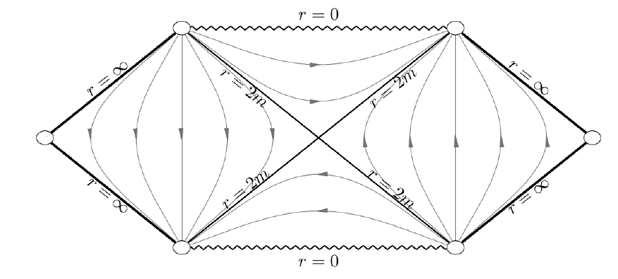
Figure 1: The Schwarzschild Penrose-Carter diagram

As is well-known, the Kruskal spacetime of mass $M>0$ outside its bifurcation surface can be covered by four patches, two of them isometric to the advanced Eddington-Finkelstein spacetime and the remaining two to the retarded Eddignton-Finkelstein. These spacetimes [Eddington, 1924, Finkelstein, 1958] consist of the manifold $\mathbb{R}\times\mathbb{R}^{+}\times\mathbb{S}^{2}$ with respective metrics

$$ds^{2} =-\left(1-\frac{M}{r}\right)dV^{2}-2\sigma dVdr+r^{2}d\Omega^{2}$$ (53)

where $\sigma=-1$ for the advanced case and $\sigma=1$ for the retarded one. The coordinates take values in $V\in\mathbb{R},r\in\mathbb{R}^{+}$ and $d\Omega^{2}$ is the round unit metric on the sphere. Furthermore the time orientation is chosen so that $V$ increases along any timelike curve. The coordinate change $V=T-\sigma r$ transforms the metric (53) into

$$ds^{2}=-dT^{2}+dr^{2}+r^{2}d\Omega^{2}+\frac{2M}{r}\left(dT-\sigma dr\right)^{2}$$

with range of variation $T\in\mathbb{R}$, $r\in\mathbb{R}^{+}$. Transforming the flat metric $dr^{2}+r^{2}d\Omega^{2}$ to Cartesian coordinates brings the metric to Kerr-Schild form

$$g=-dT^{2}+d\vec{x}\cdot d\vec{x}+\frac{2M}{r}(dr-\sigma dT)\otimes(dr-\sigma dT)$$ (54)

where $r=\sqrt{\vec{x}\cdot\vec{x}}$ and the manifold is $\mathbb{R}\times(\mathbb{R}^{3}\setminus\{0\})$. The choice of time orientation in (53) implies that the null vector field $\partial_{T}+\sigma\frac{\vec{x}}{|\vec{x}|}\partial_{\vec{x}}$ is future directed.

This form of the metric was obtained in [Kerr and Schild, 1965]. The case $\sigma=-1$ covers the upper and right quadrants of the Penrose diagram of the Kruskal spacetime depicted in Fig. 1 and hence approaches the black hole singularity at $r=0$. The case $\sigma=+1$ covers the lower and right quadrants of the diagram and approaches the white hole singularity at $r=0$. Similarly, the spacetime (54) with $\sigma=-1$ also covers the left and upper quadrants of the Kruskal diagram and the spacetime (54) with $\sigma=1$ covers the left-lower quadrants. The only set of points the Kruskal spacetime not covered by these patches is the bifurcation surface at $r=2M$.

As noticed in Remark 3, the spatial part of the geodesic equations do not depend of the choice of sign in $\sigma$ and therefore the dynamical system will also be independent of this choice. This has the following interesting consequence. Consider for instance a future directed causal geodesic stating in the region $r<2M$ in the lower part of the diagram (for simplicity we call this the white hole region and by black hole region we refer to the domain $r<2M$ in the upper part of the diagram). This geodesic can be described in the Kerr-Schild metric (54) with $\sigma=1$. After a finite value of its affine parameter, the geodesic will approach $r=2M$. This can happen with either $v\rightarrow+\infty$ or $v\rightarrow v_{0}$ finite. In either case, since the dynamical system only involves the spatial coordinates, this portion of geodesic will have a limit point $p$ in the phase space satisfying $r(p)=2M$. Irrespectively of which spacetime point $q$ is approached (even it the point lies on the bifurcation surface), the geodesic can be continued further as a portion of a geodesic in the spacetime (54) with $\sigma=-1$ having past endpoint at $q$. The fact that the dynamical system for the spatial coordinates is independent of $\sigma$ implies that the trajectory will be described in a single phase space, i.e. the change of spacetime chart will pass fully unnoticed in the phase space of the dynamical system. Thus, we will be able to describe the full geodesic as a single trajectory in the phase space, without having to determine in which spacetime coordinate chart we are working at each portion. As we will see below, this is only possible due to the presence of a excluded region in the phase space. In turn, this excluded region arises as a consequence of the restrictions in the initial data imposed by the condition that the trajectory describes a future directed causal geodesic.

5.1 Regularized dynamical system

Lemma 14.

The McGehee regularization for the dynamical system that describes the spatial part of the set of geodesic trajectories with angular momentum $L$ in the Kruskal spacetime is

$$r^{\prime} =ru,$$ (55)

$$u^{\prime} =r\left(L^{2}-\mu Mr\right)-3L^{2}M+\frac{3}{2}u^{2},$$ (56)

$$\theta^{\prime} =L\sqrt{r}.$$ (57)

where $\mu=1,0,-1$ for timelike, null and spacelike geodesics, respectively. The system admits the energy first integral

$$\epsilon=\frac{u^{2}}{2r^{3}}+\frac{L^{2}}{2r^{2}}-M\left(\frac{L^{2}}{r^{3}}+\frac{\mu}{r}\right).$$ (58)

Proof. We can apply Proposition 5 with $h=\frac{2M}{r}$, which corresponds to the spacetime (54). Equations (28), (29) and (30) become

$$\ddot{\vec{x}} =-\left(\frac{3ML^{2}}{r^{5}}+\frac{\mu M}{r^{3}}\right)\vec{x},$$ (59)

$$\vec{L} =\vec{x}\times\dot{\vec{x}},$$

$$\epsilon: =\frac{\dot{r}^{2}}{2}+\frac{L^{2}}{2r^{2}}-M\left(\frac{L^{2}}{r^{3}}+\frac{\mu}{r}\right).$$

where dot means derivative with respect to proper time, affine parameter or arc length depending on the value of $\mu$ and the energy is $E=\dot{T}\left(\frac{2M}{r}-1\right)+\frac{2M}{r}\dot{r}$, from (31).

Given a geodesic, we can rotate the Cartesian coordinates so that the geodesic lies in the plane $\{x^{1},x^{2}\}$ and define $x$ as the complex coordinate $x=x^{1}+ix^{2}$,. The equations of motion (59) become

$$\dot{x} =y,$$

$$\dot{y} =-\left(\frac{3ML^{2}}{|x|^{5}}+\frac{\mu M}{|x|^{3}}\right)x=-\nabla\left(-\frac{ML^{2}}{|x|^{3}}-\frac{\mu M}{|x|}\right):=\Lambda(|x|)x.$$

This flow is singular at $r=0$ and we can apply the McGehee regularization described above. From Corollary 12 and the fact that $|x|^{3}V(|x|)$ admits a $C^{1}$ extension to $x=0$ with non-zero value at this point, we find that the optimal value for regularization is $\beta=\mbox{min}\{-1,-\frac{\gamma}{2}\}=-\frac{3}{2}$. Applying Lemma 11 the following regularized system is obtained

$$r^{\prime} =ru$$

$$u^{\prime} =r\left(L^{2}-\mu Mr\right)-3L^{2}M+\frac{3}{2}u^{2}$$

$$\theta^{\prime} =L\sqrt{r}$$

$$\epsilon =\frac{u^{2}}{2r^{3}}+\frac{L^{2}}{2r^{2}}-M\left(\frac{L^{2}}{r^{3}}+\frac{\mu}{r}\right).$$

$\blacksquare$

5.1.1 Excluded regions

The dynamical system (55)-(57) describes all future directed causal geodesics in the Kruskal spacetime. However, not all trajectories in this dynamical system correspond to future directed causal geodesics in this spacetime. The reason is that the set of initial data $\{r_{0},\dot{r}_{0}\}$ for future directed causal geodesics is constrained by Proposition 5. Given the relation between $u$ and $\dot{r}$, this implies that not all points $\{r,u,\theta\}$ in the phase space describe future causal geodesics in the spacetime. We will call the allowed region the set of points in the phase space corresponding to future directed causal geodesics and the excluded region its complement. Let us determine these sets.

As discussed in Proposition 5, at points where $h<1$, i.e. $r>2M$, there is no restriction on the possible values of $\dot{r}_{0}$, and consequently no restrictions on $u$ arise. On the other hand, when $h>1$, i.e. $r<2M$, then

$$\sigma\dot{r}_{0}\in[a_{0},\infty)$$

where

$$a_{0}=\sqrt{\left(\frac{2M}{r}-1\right)\left(\frac{L^{2}}{r^{2}}+\mu\right)}.$$

For $h=1$ ($r=2M$), $\dot{r}_{0}$ is restricted to satisfy

$$\sigma\dot{r}_{0}\in[0,\infty)$$

with $\dot{r}_{0}=0$ only if $L=0$ and the geodesic is null ($\mu=0$). Given that $u=r^{-\beta}\dot{r}=r^{\frac{3}{2}}\dot{r}$ the allowed region for geodesics in the advanced Eddington-Finkelstein spacetime (i.e. $\sigma=-1$) is

$$u\in\left(-\infty,-r^{\frac{3}{2}}\sqrt{\left(\frac{2M}{r}-1\right)\left(\frac{L^{2}}{r^{2}}+\mu\right)}\,\right], r\leq 2M$$

$$\mbox{with }(u=0,r=2M)\mbox{ allowed only if }L=0,\mu=0,$$

$$u\in(-\infty,\infty) r>2M$$

So, the excluded region is

$$u\in\left(-r^{\frac{3}{2}}\sqrt{\left(\frac{2M}{r}-1\right)\left(\frac{L^{2}}{r^{2}}+\mu\right)},\infty\right),\quad\quad r\leq 2M$$

$$\mbox{with }(u=0,r=2M)\mbox{ excluded if }L\neq 0\mbox{ or }\mu\neq 0$$

Similarly, for geodesics in the retarded Eddington-Finkelstein spacetime ($\sigma=1$) the excluded region is

$$u\in\left(-\infty,r^{\frac{3}{2}}\sqrt{\left(\frac{2M}{r}-1\right)\left(\frac{L^{2}}{r^{2}}+\mu\right)}\right),\quad\quad r\leq 2M$$

$$\mbox{with }(u=0,r=2M)\mbox{ excluded if }L\neq 0\mbox{ or }\mu\neq 0.$$

As discussed above, the bifurcation surface at $r=2M$ is not included in either the advanced or retarded Eddington-Finkelstein spacetime. This is the reason why the the point $(u=0,r=2M)$ when either $L\neq 0$ or $\mu\neq 0$ is excluded. Since future causal geodesics with $L\neq 0$ in the Kruskal spacetime do cross the bifurcation surface, we must incorporate this set of points of the phase space into the allowed region in order to describe all causal geodesics of the Kruskal spacetime. We conclude that the set of phase space points not describing future directed causal geodesics in the Kruskal spacetime is the intersection of both excluded regions after adding $(u=0,r=2M)$ to the allowed regions, namely

$$u \in\left(-r^{\frac{3}{2}}\sqrt{\left(\frac{2M}{r}-1\right)\left(\frac{L^{2}}{r^{2}}+\mu\right)},r^{\frac{3}{2}}\sqrt{\left(\frac{2M}{r}-1\right)\left(\frac{L^{2}}{r^{2}}+\mu\right)}\right),\quad\quad r\leq 2M.$$

The existence of these three types of excluded regions is crucial for describing all future directed causal geodesics in the Kruskal spacetime in a single phase space diagram. Indeed, any trajectory passing through an allowed point in the region $r<2M$ with $u>0$ belongs to the $r<2M$ region of a retarded Eddington-Finkelstein chart of the Kruskal spacetime, i.e. to the white hole region of the spacetime. A trajectory passing through an allowed point in the region $r<2M$ with $u>0$, belongs to an advanced Eddignton-Finkelstein chart of the Kruskal spacetime, i.e. to the black hole region. A point in the phase space with $r>2M$ belongs to both charts.

The boundary of the allowed region is given by the set of points satisfying

$$u^{2}=r^{3}\left(\frac{2M}{r}-1\right)\left(\frac{L^{2}}{r^{2}}+\mu\right),\quad\quad r\leq 2M$$

which can be rewritten as the set of points with $\epsilon=-\frac{\mu}{2}$. In fact, the excluded region can be equivalently defined as the set of points for which $\epsilon<-\frac{\mu}{2}$, $r\leq 2M$, cf. Corollary 7.

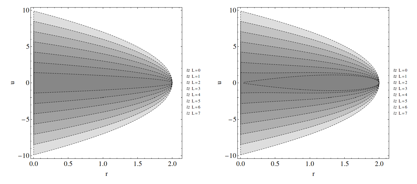
Figure 2: The left image correspond to the excluded regions in the phase space $\{r,u\}$ for null geodesics ($\mu=0$). Different values of the angular momentum $L$ are displayed (the darker the zone, the lower the value of $L$). The right image corresponds to the analogous case for timelike geodesics ($\mu=1$). In both cases $M=1$.

The graphical representation of the excluded regions for null and spacelike geodesics is displayed in Fig. 2. Notice that, in the null case, there is no excluded region in the limit $L=0$. However, in this case the set of points $u=0$ correspond to trivial null geodesics consisting of single points with vanishing tangent vector. For non- null geodesics, the excluded region is always non-empty irrespectively of the value of the angular momentum $L$.

5.2 The collision manifold

              

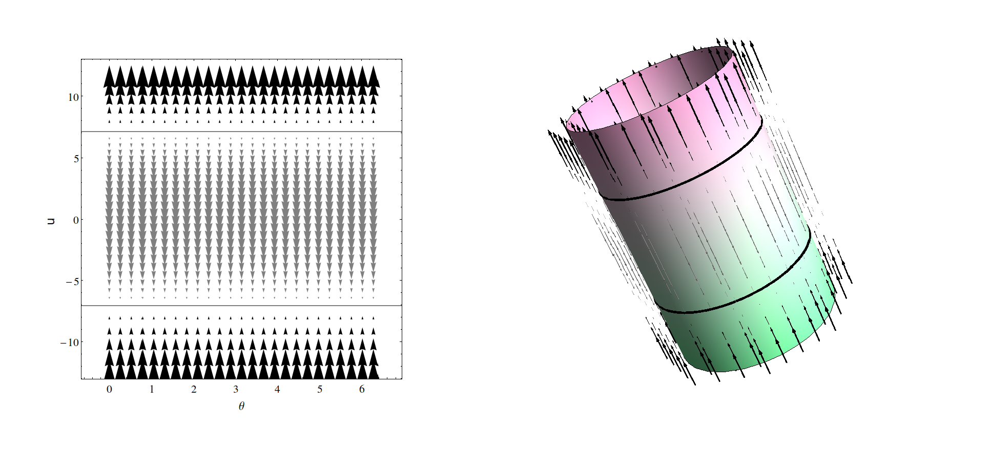
Figure 3: The flow in the collision manifold (left) with the critical lines in $u=\pm\sqrt{2M}L$ (we have chosen $L=5,M=1$) and the collision manifold embedded cylinder (right) with the flow and the critical lines over it.

The submanifold $r=0$ is clearly invariant under the flow. Since $r=0$ corresponds to the spacetime singularity, this submanifold is called collision manifold. It can be described globally by the coordinates $\{(\theta,u)\}$ so its topology is $\mathbb{R}\times\mathbb{S}^{1}$. The dynamical system (56)-(57) restricted to the collision manifold reads

$$u^{\prime} =\frac{3}{2}u^{2}-3L^{2}M,$$

$$\theta^{\prime} =0.$$

This system has two lines of critical points: one line of stable points at $(\theta,u)=(\theta_{0},-\sqrt{2ML^{2}})$ and one line of unstable nodes at $(\theta,u)=(\theta_{0},\sqrt{2ML^{2}})$, where $\theta_{0}\in\mathbb{S}^{1}$ is an arbitrary value. The phase space portrait in the collision manifold is shown in Fig. 3. For each value of $\theta_{0}$, there is a trajectory extending from $u=-\infty$ and approaching $u=-\sqrt{2ML^{2}}$ as its future limit point, a trajectory from $u=-\sqrt{2ML^{2}}$ to $u=\sqrt{2ML^{2}}$ and a trajectory having $u=\sqrt{2ML^{2}}$ as its past limit point and extending to $u=+\infty$, all of them with $\theta=\theta_{0}$. One may wonder how these trajectories relate to causal geodesics in the Kruskal spacetime. To see this, note that any such geodesics must have a finite value of $\epsilon$. On the other hand $\epsilon$ diverges at $r=0$ (see (58)). In fact, it does so in the following way

$$\lim_{r\rightarrow 0}\epsilon=\left\{\begin{array}[]{l}+\infty\quad\quad\mbox{if}\quad|u|>\sqrt{2ML^{2}},\\ -\infty\quad\quad\mbox{if}\quad|u|<\sqrt{2ML^{2}}.\\ \end{array}\right.$$

The limit when $|u|$ approaches the critical points on the collision manifold depends on the details of how this limit is taken. Since, the trajectories joining the stable critical points to the unstable ones within the collision manifold are interior to the excluded region of the phase phase, it follows that such trajectories are completely unrelated to causal geodesics in the spacetime. This is consistent with the fact that $\epsilon\rightarrow-\infty$ on these trajectories, while future directed causal geodesics in the region $r<2M$ must have $\epsilon\geq-\frac{\mu}{2}$. On the other hand, the trajectories on the collision manifold leaving $u=+\sqrt{2ML^{2}}$ and those approaching $u=-\sqrt{2ML^{2}}$ correspond to the limit of trajectories of causal geodesics leaving the white hole singularity at $r=0$ and approaching the black hole singularity at $r=0$ when their energy $\epsilon$ diverges to $+\infty$. Thus, this set of trajectories on the collision manifold carries interesting information on the causal geodesics in the spacetime.

To analyze the behavior of the particles near the collision manifold, we can linearize the system at its first order as

$$r(s) =\delta r(s),$$

$$u(s) =u_{0}(s)+\delta u(s),$$

where $u_{0}(s)$ its a solution that corresponds to an orbit in the collision manifold and therefore satisfies

$$u_{0}^{\prime}=-3L^{2}M+\frac{3u_{0}^{2}}{2}.$$

The general solution for this differential equation satisfying $|u_{0}|>\sqrt{2ML^{2}}$ is

$$u_{0}(s)=-\sqrt{2ML^{2}}\coth\left(3\sqrt{\frac{ML^{2}}{2}}s\right).$$

The branch $s\in(-\infty,0)$ corresponds to the solution leaving the unstable fixed point at $u=+\sqrt{2ML^{2}}$ and approaching $u\longrightarrow+\infty$, while the branch $s\in(0,+\infty)$ corresponds to the solution extending from $u=-\infty$ and approaching the fixed point $u=-\sqrt{2ML^{2}}$. The first-order linearized system in the variables $\delta r$ and $\delta u$ is

$$\delta r^{\prime} =(\delta r)u_{0},$$

$$\delta u^{\prime} =L^{2}(\delta r)+3(\delta u)u_{0}.$$

We can easily solve for $\delta r(s)$:

$$\delta r(s)=\frac{\delta r_{0}}{\left|\sinh\left(3\sqrt{\frac{ML^{2}}{2}}s\right)\right|^{\frac{2}{3}}},$$

where $\delta r_{0}>0$ is an arbitrary integration constant. Thus, the fixed points are approached exponentially fast in the variable $s$. To analyze the behavior in the $\tau$ variable we recall the relation (42), namely

$$\tau^{\prime}(s)=(\delta r(s))^{\frac{5}{2}}.$$

This integration can be performed explicitly, but it is not particularly enlightening. Instead, we will determine a series expansion of $\delta r(\tau)$ near $\tau=0$ where $\tau$ is chosen so that the particle reaches the singularity $r=0$ at $\tau=0$ (note that $\tau<0$ for particles approaching the black hole singularity while $\tau>0$ for particles leaving the white hole singularity). Define $x(s)$ as

$$x(s)=\frac{1}{\left|\sinh\left(3\sqrt{\frac{ML^{2}}{2}}\,s\right)\right|^{\frac{2}{3}}}$$

so that $(\delta r)(s)=(\delta r_{0})x(s)$ and hence $\frac{dx}{ds}=u_{0}x$. In terms of $x$,

$$u_{0}=\mp\sqrt{2ML^{2}}\sqrt{1+x^{3}},$$

where the sign depends on the branch we are considering (upper sign for the approach to the black hole and lower sign for the white hole). Then

$$\frac{d\tau}{dx}=\frac{d\tau}{ds}\frac{ds}{dx}=\frac{(\delta r_{0}\,x)^{\frac{5}{2}}}{xu_{0}}=\mp\frac{(\delta r_{0})^{\frac{5}{2}}}{\sqrt{2ML^{2}}}\frac{x^{\frac{3}{2}}}{\sqrt{1+x^{3}}}.$$

Expanding the right-hand side as a series en $x$, integrating and inverting we find

$$x(\tau)=\left(\frac{5}{2}\right)^{\frac{2}{5}}\left(\mp a\tau\right)^{\frac{2}{5}}+\frac{5}{22}\left(\frac{5}{2}\right)^{\frac{3}{2}}\left(\mp a\tau\right)^{\frac{8}{5}}+O(\tau^{\frac{18}{5}})+\dots$$

where $a=\frac{\sqrt{2ML^{2}}}{(\delta r_{0})^{\frac{5}{2}}}$. A plot of the function $\delta r(\tau)$ in each of the two branches is given in Fig. 4. These plots describe the approach to the singularity of very energetic particles in the Kruskal spacetime for different values of the angular momentum. Note that the result is the same for massive and massless particles, as one could expect given the very high energy involved.

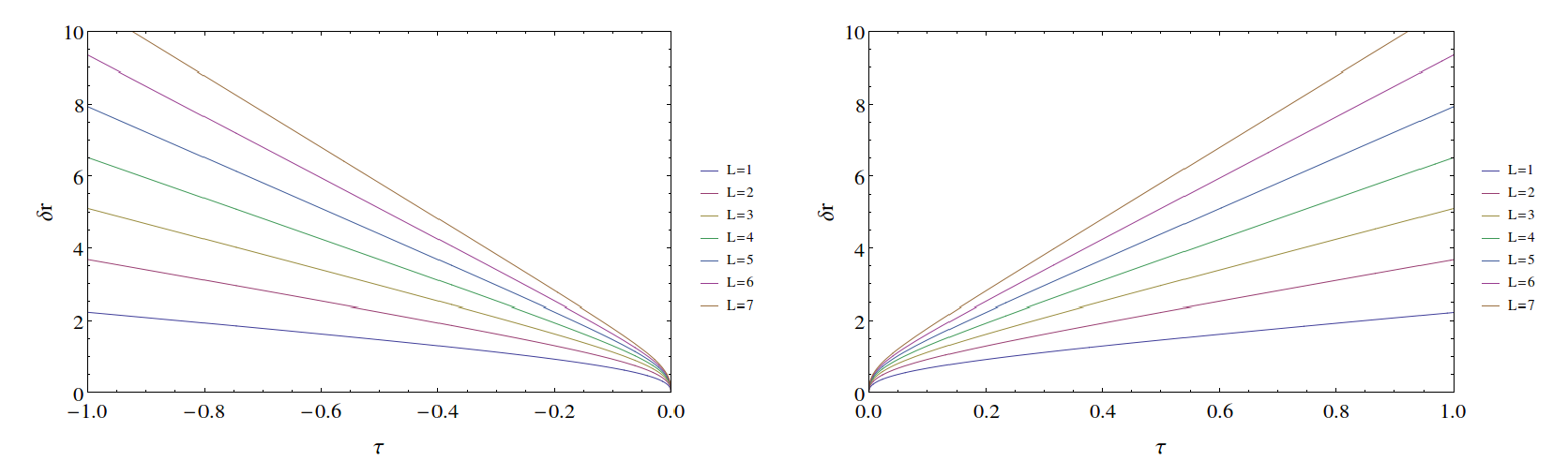
Figure 4: Plot of the function $\delta r(\tau)$. The image on the left corresponds to the branch in witch $u_{0}\leq-\sqrt{2ML^{2}}$ (black hole solution) in the collision manifold and the image on the right corresponds to the branch in witch $u_{0}\geq\sqrt{2ML^{2}}$ (white hole solution). In both plots $\delta r_{0}=1$ and $M=1$.

5.3 The general flow

5.3.1 Massless particles

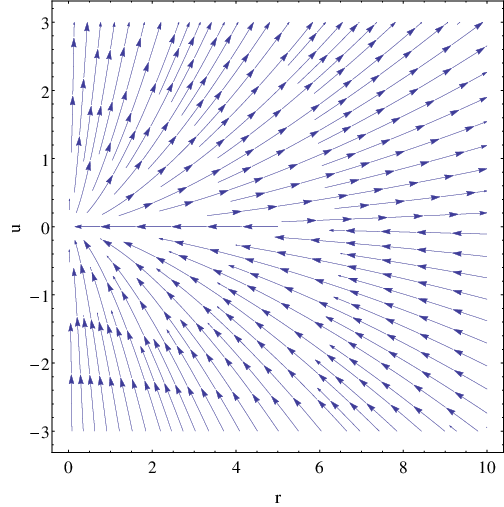
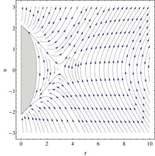
Figure 5: Phase space for massless particles with $L=0$ (left picture) and $L=1.5M$ (right picture). The dark zone correspond to the forbidden region given by $\epsilon<\frac{\mu}{2}$.

The reduced dynamical system with $\mu=0$ takes the form

$$r^{\prime} =r\,u,$$ (61)

$$u^{\prime} =rL^{2}-3L^{2}M+\frac{3u^{2}}{2}.$$ (62)

Its phase space is displayed for different values of $L$ in Fig. 5. The fixed points are (assuming $L\neq 0$)

$$(r=0,u=\pm\sqrt{2M}L)\quad\quad(r=3M,u=0).$$

The linearization of the system around these points has the following eigenvalues

$$\begin{cases}\lambda_{1}=\sqrt{3ML^{2}},\quad\lambda_{2}=-\sqrt{3ML^{2}}&\mbox{for }\quad(r=3M,u=0),\\ \lambda_{1}=\pm 3\sqrt{2ML^{2}}\quad\lambda_{2}=\pm\sqrt{2ML^{2}}&\mbox{for}\quad(r=0,u=\pm\sqrt{2M}L).\end{cases}$$

Thus, all critical points are hyperbolic. The point $(r=0,u=+\sqrt{2ML^{2}})$ is an unstable node (repulsor), $(r=0,u=-\sqrt{2ML^{2}})$ is a stable node (attractor) and $(r=3M,u=0)$ is saddle point. This saddle point obviously corresponds to the unstable circular orbit for massless particles.

5.3.2 Massive particles

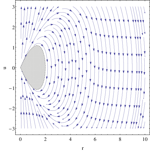
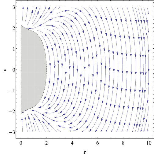
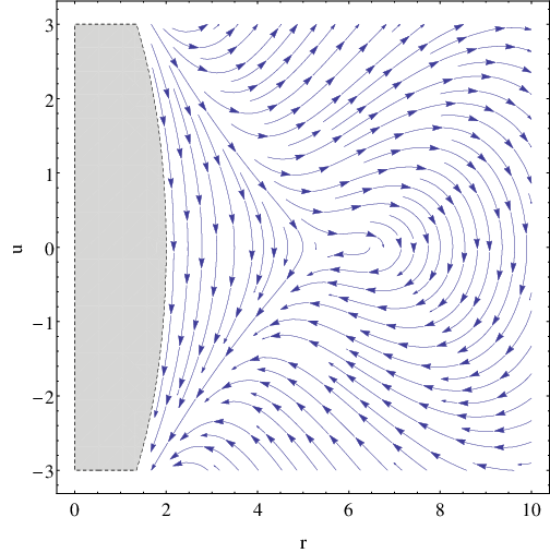
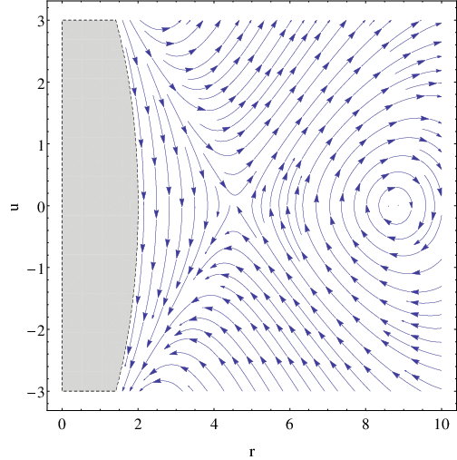
Figure 6: Phase spaces for massive particles with $L=0$, $L=1.5M$, $L=2\sqrt{3}M$ and $L=3.65M$. The dark zone correspond to the forbidden region given by $\epsilon<\frac{\mu}{2}$. The larger the value of $L/M$ the larger the excluded region in the phase space.

When $\mu=1$ the reduced dynamical system is

$$r^{\prime} =r\,u,$$

$$u^{\prime} =r\left(L^{2}-Mr\right)-3L^{2}M+\frac{3u^{2}}{2},$$

with phase spaces displayed for different values of $L$ in Fig. 6. The fixed points are

$$(r=0,u=\pm\sqrt{2ML^{2}}),\quad\quad(r=r_{\pm}(M,|L|):=\frac{L^{2}\pm|L|\sqrt{L^{2}-12M^{2}}}{2M},u=0),$$

the second pair under the additional condition $L^{2}\geq 12M^{2}$. For $L^{2}>12M^{2}$ all fixed points are hyperbolic, with $(r=r_{+}(M,|L|),u=0)$ being a center (purely imaginary eigenvalues) and $(r=r_{-}(M,|L|),u=0)$ being a saddle. When $L^{2}=12M^{2}$, there is a bifurcation in the phase space, which can be visualized in the transition between the third and fourth plots in Fig. 6. Given that $r_{+}(M,|L|)$ is an increasing function of $|L|$ with values ranging from $(6M,\infty)$ we recover the well-known fact that the innermost stable circular orbit (ISCO) in Schwarzschild is $r=6M$. The fixed point $r_{-}(M,|L|)$ is a decreasing function of $|L|$ with values ranging from $6M$ (when $|L|\rightarrow 2\sqrt{3}M$) to $3M$ when $|L|\rightarrow+\infty$). We thus recover easily all well-known results for geodesics in Schwarzschild outside the horizon. The approach here, however, is perfectly regular both across the horizon at $r=2M$ and even at the singularity $r=0$. Moreover, it allows us to treat all points in the Kruskal spacetime with a single dynamical system.

6 The Reissner–Nordström dynamical system

The Reissner–Nordström spacetime [Reissner, 1916, Nordström, 1918] corresponds to the most general solution for Einstein equations with electromagnetic field when spherical symmetry is assumed. The maximal extension of this spacetime is covered by a infinite amount of copies of four basic patches. As in the Kruskal spacetime two of the patches are isometric to the Reissner–Nordström advanced Eddington-Finkelstein spacetime and the remaining two to the Reissner–Nordström retarded Eddignton-Finkelstein. Each one of these spacetimes consist of the manifold $\mathbb{R}\times\mathbb{R}^{+}\times\mathbb{S}^{2}$ with respective metrics

$$ds^{2}=-\left(1-\frac{2M}{r}+\frac{Q^{2}}{r^{2}}\right)dV^{2}-2\sigma dVdr+r^{2}d\Omega^{2},$$

where $\sigma=-1$ for the advanced case and $\sigma=1$ for the retarded one. The coordinates takes values in $V\in\mathbb{R},r\in\mathbb{R}^{+}$ and $d\Omega^{2}$ is the round unit metric on the sphere. Performing the same coordinate change as in the Kruskal case, the metric is transformed into its Kerr-Schild form [Kerr and Schild, 1965]:

$$g=-dT^{2}+d\vec{x}\cdot d\vec{x}+\frac{2Mr-Q^{2}}{r^{2}}(dr-\sigma dT)\otimes(dr-\sigma dT)$$ (63)

where $r=\sqrt{\vec{x}\cdot\vec{x}}$ and the manifold is $\mathbb{R}\times(\mathbb{R}^{3}\setminus\{0\})$. As before we choose the orientation so that the nowhere-zero, null vector $\partial_{T}+\sigma\frac{\vec{x}}{|\vec{x}|}\partial_{\vec{x}}$ is future directed.

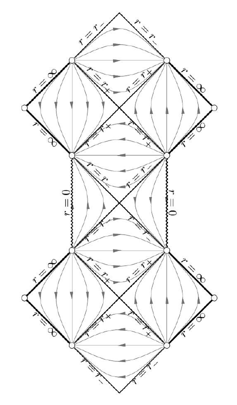
Figure 7: The Reissner–Nordström Penrose-Carter diagram.

As is well-known, the global structure of the maximal extension of the Reissner-Nordström spacetime depends strongly on whether $|Q|>M$, $|Q|=M$ or $|Q|<M$. For the discussion below we concentrate on the latter case because it corresponds to a non-extremal black hole. We emphasize, however, that all the dynamical systems in this Section are valid for any value of $Q$ and $M$, so they can be used to study geodesics in the extremal black hole or naked singularity cases as well.

When $|Q|<M$, the basic structure of the maximal extension of the Reissner–Nordström spacetime has now two bifurcation surfaces located, respectively, at the intersection of the two smooth null hypersurfaces with $r=r_{+}$ and the two smooth null hypersurfaces with $r=r_{-}$, where $r_{\pm}=M\pm\sqrt{M^{2}-Q^{2}}$. We call each one of these four hypersurfaces a horizon. The patch with $\sigma=-1$ covers the structure unit that goes in ascending way from $r=\infty\to r=r_{+}\to r=r_{-}\to r=0$ (starting from either the right or the left) while the patch with $\sigma=1$ covers the structure unit that goes in an ascending way from $r=0\to r=r_{-}\to r=r_{+}\to r=\infty$ (starting from the right or the left). Notice that there is no causal geodesic starting from a left-most quadrant which, after crossing the null hypersurface $r=r_{+}$ then goes across the portion of the null hypersurface at $r=r_{-}$ lying at the left of the diagram (and similarly for geodesics starting at a right-most quadrant). The reason is that the Killing 1-form $\mbox{\boldmath$\xi$}:=g(\xi,\cdot)$ where $\xi=\partial_{T}$ (defined on a single Eddington-Finkelstein patch) is integrable with orthogonal hypersurfaces foliating the region $r_{-}<r<r_{+}$ with timelike leaves. Let us label these leaves by $t$. As a consequence we have $\mbox{\boldmath$\xi$}=Gdt$ on $r_{-}<r<r_{+}$ where $G$ is a smooth function. Consider the conserved energy for the geodesic, i.e. $\langle\partial_{T},u\rangle=-E$ where $u$ is the tangent vector. In the region between $r_{-}$ and $r_{+}$, in order for the geodesic to enter from the left portion of the null hypersurface $r=r_{+}$ and leave across the left portion of the hypersurface $r=r_{-}$, the geodesic must become somewhere tangent to a hypersurface $t=\mbox{const}$. At this point we have $-E=\mbox{\boldmath$\xi$}(u)=Gdt(u)=0$. But $E=0$ is impossible for a geodesic starting on the left-most region where $\xi$ is timelike. A similar argument applies to geodesics starting at the right-most quadrant.

As discussed in Section 5, the fact that the dynamical system for the spatial coordinates is independent of $\sigma$ implies that the trajectory will be described in a single phase space. To understand the geodesic flow along the maximal extension of the Reissner–Nordström we need to analyze the excluded regions. We first write down the regularized dynamical system.

6.1 Regularized dynamical system

Lemma 15.

The McGehee regularization for the dynamical system that describes the spatial part of the set of geodesic trajectories with angular momentum $L$ in the Kruskal spacetime is

$$r^{\prime} =ru,$$ (64)

$$\theta^{\prime} =L\,r,$$ (65)

$$u^{\prime} =r\left(r\left(L^{2}-\mu Mr+\mu Q^{2}\right)-3L^{2}M\right)+2\left(L^{2}Q^{2}+u^{2}\right).$$ (66)

where $\mu=1,0,-1$ for timelike, null and spacelike geodesics, respectively. The system admits the energy first integral

$$L^{2}\left(r(r-2M)+Q^{2}\right)+\mu r^{2}\left(Q^{2}-2Mr\right)+u^{2}=2r^{4}\epsilon.$$ (67)

Proof. We can apply Proposition 5 with $h=\frac{2Mr-Q^{2}}{r^{2}}$, from (63). Equations (28), (29) and (30) become

$$\ddot{\vec{x}} =\left(\left(\frac{2Q^{2}L^{2}}{r^{6}}+\frac{\mu Q^{2}}{r^{4}}\right)-\left(\frac{3ML^{2}}{r^{5}}+\frac{\mu M}{r^{3}}\right)\right)\vec{x},$$

$$\vec{L} =\vec{x}\times\dot{\vec{x}},$$

$$\epsilon: =\frac{\dot{r}^{2}}{2}+\frac{L^{2}}{2r^{2}}-M\left(\frac{L^{2}}{r^{3}}+\frac{\mu}{r}\right)+Q^{2}\left(\frac{L^{2}}{2r^{4}}+\frac{\mu}{2r^{2}}\right).$$

Adapting coordinates so that the geodesic lies in the $\{x^{1},x^{2}\}$ plane and defining the complex variable $x=x^{1}+ix^{2}$, the equations are

$$\dot{x} =y,$$

$$\dot{y} =\left(\left(\frac{2Q^{2}L^{2}}{|x|^{6}}+\frac{\mu Q^{2}}{|x|^{4}}\right)-\left(\frac{3ML^{2}}{|x|^{5}}+\frac{\mu M}{|x|^{3}}\right)\right)x$$

$$=-\nabla\left(-M\left(\frac{L^{2}}{|x|^{3}}+\frac{\mu}{|x|}\right)+Q^{2}\left(\frac{L^{2}}{2|x|^{4}}+\frac{\mu}{2|x|^{2}}\right)\right):=\Lambda(|x|)x.$$

We now apply the McGehee regularization. Since $|x|^{4}V(|x|)$ admits a $C^{1}$ extension to $x=0$, Corollary 12 fixes the optimal value for regularization as $\beta=\mbox{min}\{-1,-\frac{\gamma}{2}\}=-2$ and Lemma 11 gives the regularized system (64)-(66) as well as the constant of motion $\epsilon$. $\blacksquare$

6.1.1 Excluded regions

As in the Schwarzschild case, not all trajectories of the dynamical system (64)-(66) correspond to future directed causal geodesics in the Reissner-Nordström spacetime. Proceeding as in Schwarzschild and exploiting Proposition 5, it is straightforward to find that the excluded region of the phase space diagram is

$$u \in\left(-r^{2}\sqrt{\left(\frac{2M}{r}-\frac{Q^{2}}{r^{2}}-1\right)\left(\frac{L^{2}}{r^{2}}+\mu\right)},r^{2}\sqrt{\left(\frac{2M}{r}-\frac{Q^{2}}{r^{2}}-1\right)\left(\frac{L^{2}}{r^{2}}+\mu\right)}\right),\quad\quad r_{-}\leq r\leq r_{+}.$$

In addition, for geodesics in the $\sigma=-1$ Eddington-Finkelstein patch $u$ must be lie below the forbidden region (i.e. $u\leq 0$ in the strip $r_{-}\leq r\leq r_{+}$), while geodesics in the $\sigma=+1$ Eddington-Finkelstein patch must lie above the forbidden region (i.e. $u\geq 0$ in the strip $r_{-}\leq r\leq r_{+}$ ). Note that, as in Schwarzschild, the boundary of the allowed region is defined by

$$u^{2}=r^{4}\left(\frac{2M}{r}-\frac{Q^{2}}{r^{2}}-1\right)\left(\frac{L^{2}}{r^{2}}+\mu\right),\quad\quad r_{-}\leq r\leq r_{+},$$

which correspond to the set of points with $\epsilon=-\frac{\mu}{2}$ and the excluded region is precisely the set $\epsilon<-\frac{\mu}{2}$, $r_{-}\leq r\leq r_{+}$, cf. Corollary 7.

The excluded regions for timelike geodesics are displayed in Fig. 8 with representative values of $Q$ and $L$. The excluded regions for timelike/null geodesics show the same behavior on $L$ as in the Schwarzschild case, i.e. in the null case there is no excluded region in the limit $L=0$ but then the line $u=0$ consists of a family of trivial geodesics and in the timelike case the excluded region is always non-empty for all values of $L$.

We can now discuss how the behavior of geodesics across the horizons can be described in the phase space diagram. The crucial information is the restriction for $u$ (which, recall, is proportional to $\dot{r}$) in the domain $r_{-}<r<r_{+}$. Let us see how this implies that any geodesic traveling from $r=r_{0}>r_{+}\to r_{+}\to r_{-}\to r_{1}$ and back to $r_{-}\to r_{+}$ must have changed the Kerr-Schild patch along the way (by changing the value of $\sigma$). Assume for definiteness that the particle starts in a left-most quadrant. After the crossing of $r_{+}$ the particle must necessarily cross $r=r_{-}$. This well-known fact can be directly deduced also from the dynamical system because the allowed region in the domain $r_{-}<r<r_{+}$ when $\sigma=-1$ has $u<0$ everywhere. The crossing of $r=r_{-}$ happens in the right part of the Kerr-Schild patch, as discussed before. Thus the trajectory is still contained in the original Kerr-Schild patch and, at the same time, it has also entered a new patch with $\sigma=-1$. Since the collision manifold cannot be attained (see below) the geodesic must necessarily reach a point where $u=0$ and cross to positive values of $u$. From then on, the curve crosses $r=r_{-}$ towards larger values of $r$. At this crossing, the trajectory necessarily leaves the original Kerr-Schild patch. It does so with $u>0$ which is compatible with the fact that we now have $\sigma=-1$ and hence the allowed region lies above the forbidden bubble. The geodesic necessarily crosses $r=r_{+}$ and enters a different asymptotic region from which it started. This behavior is of course well-known. What is important here is that a single phase space allows for a complete description of the complicated spacetime trajectory by simply noticing that each time that the forbidden region is encircled, we have moved one step in the ladder in Kerr-Schild patches in the maximal extension of Reissner-Nordström. This is possible only because (i) the phase space has an excluded region and (ii) the crossing at $r=r_{-}$ is not ambiguous, forcing the particle to stay in the same Kerr-Schild patch it started.

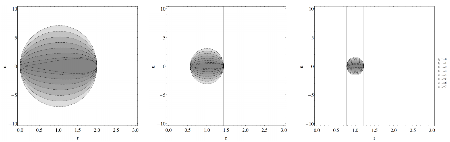
Figure 8: The three pictures displayed correspond to the excluded regions in the phase space $\{r,u\}$ for timelike geodesics ($\mu=1$) with $Q=0$, $Q=0.9$ and $Q=0.975$ respectively. Different values of the angular momentum $L$ are displayed in each one (the darker the zone, the lower the value of $L$). Units are chosen so that $M=1$. The vertical lines correspond to $r_{\pm}$.

6.2 The collision manifold

The Reissner-Nordström collision manifold has again topology $\mathbb{R}\times\mathbb{S}^{1}$ and global coordinates $\{(\theta,u)\}$. The dynamical system (65)-(66) restricted to the collision manifold reads

$$u^{\prime} =2\left(L^{2}Q^{2}+u^{2}\right),$$

$$\theta^{\prime} =0,$$ (68)

which has no fixed points. This is a manifestation of the fact that, in Reissner-Nordström, the singularity has a repulsive behavior, unlike the Schwarzschild case. This is already indicated by the fact that, for $|LQ|\neq 0$, $\lim_{r\rightarrow 0}\epsilon=+\infty$ irrespective of the value of $u$. So, no physical particles with finite energy can access the collision manifold and, the larger the value of $\epsilon$ they have, the closer to the collision manifold $r=0$ they can get.

To analyze the repulsive nature of the collision manifold in more detail let us linearize the dynamical system to its first order around the collision manifold. Thus, we write

$$r(s) =\delta r(s),$$

$$u(s) =u_{0}(s)+\delta u(s),$$

where $u_{0}(s)$ is a trajectory on the collision manifold, so that it satisfies

$$u_{0}^{\prime}=2L^{2}Q^{2}+2u^{2}.$$

The general solution for this differential equation satisfying $u_{0}(0)=-\infty$ is

$$u_{0}(s)=-|LQ|\cot(2|LQ|s).$$

Where $s\in(0,\frac{\pi}{2|LQ|})$. The first-order linearized system in the variables $\delta r$ and $\delta u$ is

$$\delta r^{\prime} =(\delta r)u_{0},$$

$$\delta u^{\prime} =-3L^{2}M\delta r+4(\delta u)u_{0}.$$

We can easily solve for $\delta r(s)$:

$$\delta r(s)=\frac{\delta r_{0}}{\sqrt{\sin(2|LQ|s)}},$$

where $\delta r(\frac{\pi}{4|LQ|})=\delta r_{0}$. If follows that, no matter how close to the collision manifold we get (at $s=\frac{\pi}{4|LQ|}$ where $\delta r(s)$ is minimum), the trajectory never touches the collision manifold and in fact, it separates from it very quickly. To understand how fast this happens we need to change to the $\tau$ variable. Given the relation (42), namely

$$\tau^{\prime}(s)=(\delta r(s))^{3}.$$

As in the Schwarzschild case we will determine a series expansion of $\delta r(\tau)$ near $\tau=0$, where $\tau$ is chosen to fulfill $\tau=0$ when $s=\frac{\pi}{4|LQ|}$. Define $x(s)$ as

$$x(s)=\frac{1}{\sqrt{\sin(2|LQ|s)}}$$

so that $(\delta r)(s)=(\delta r_{0})x(s)$ and hence $\frac{dx}{ds}=u_{0}x$. In terms of $x$

$$u_{0}=-|LQ|\sqrt{x^{4}-1},$$

then

$$\frac{d\tau}{dx}=\frac{d\tau}{ds}\frac{ds}{dx}=\frac{(\delta r_{0}\,x)^{3}}{u_{0}x}=-\frac{(\delta r_{0})^{3}}{|LQ|}\frac{x^{2}}{\sqrt{x^{4}-1}}.$$

Expanding the right-hand side as a series en $x$, integrating and inverting we find

$$x(\tau)=1+(a\tau)^{2}-\frac{5}{6}(a\tau)^{4}+\frac{23}{18}(a\tau)^{6}+O(\tau)^{8}$$

where $a=\frac{|LQ|}{(\delta r_{0})^{3}}$.

It is interesting to note that inserting $Q=0$ in (68) we do not recover the Schwarzschild case. This is because the value of the parameter $\beta$ adapted to Reissner-Nordström is different to that of Schwarzschild. Thus, in the Schwarzschild subcase of Reissner-Nordström we have overkilled the singularity and the fixed points that previously existed at $r=0$, $u=u_{\pm}$ have both collapsed to $u=0$. This collapse can be detected directly on the Reissner-Nordström phase space because the fixed point $\{u=0,\theta=\theta_{0}\}$ is no longer hyperbolic when $Q=0$. Another way of seeing this is by comparing the shape of the excluded regions of phase space $\{r,u\}$ for $Q=0$ with the shape of the excluded regions in the Schwarzschild phase space. While in the latter case the excluded regions covered a non-empty interval of $\{r=0\}$, the Reissner-Nordström regularization is such that the bubble displayed in Fig. 8 , which stays separated from the collision manifold when $Q\neq 0$, just touches the line $\{r=0\}$ in the limit $Q=0$. Thus the whole line of excluded points in the Schwarzschild regularization has collapsed to a point in the Reissner-Nordström regularization of the Schwarzschild spacetime.

6.3 The general flow

6.3.1 Massless particles

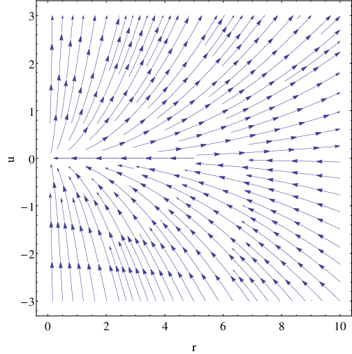
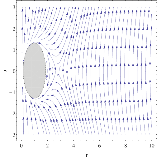
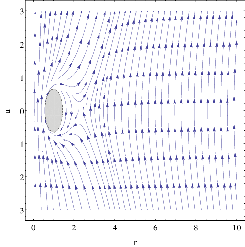
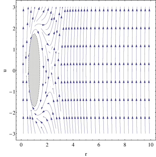
Figure 9: Phase space for massless particles for the values ($L=0$, $Q=0$) , ($L=1.5M$, $Q=0.5M$), ($L=1.5M$, $Q=0.9M$) and ($L=4M$, $Q=0.9M$) from left to right. The dark zone corresponds to the forbidden region.

The reduced dynamical system when $\mu=0$ is

$$r^{\prime} =ru$$

$$u^{\prime} =r\left(L^{2}r-3L^{2}M\right)+2\left(L^{2}Q^{2}+u^{2}\right).$$

The phase portrait can be viewed for different values of $L$ and $Q$ in Fig. 9. The fixed points of this system (assuming $LQ\neq 0$) are

$$(r=R_{\pm}(M,Q):=\frac{1}{2}\left(3M\pm\sqrt{9M^{2}-8Q^{2}}\right),u=0)$$

provided $0<|Q|\leq\sqrt{\frac{9}{8}}M$. In the strict inequality case, the two fixed points are hyperbolic, with the point $(u,r)=(0,R_{+}(M,Q))$ being a saddle point (with real eigenvalues of opposite sign) and the point $(u,r)=(0,R_{-}(M,Q))$ being a center (purely imaginary eigenvalues). It is straightforward to check that the point $(u=0,r=R_{+}(M,Q))$ always lies in the allowed region. The point $(u=0,r=R_{-}(M,Q))$ lies in the excluded region as soon as this region is non-empty, i.e. for $|Q|<M$.

As discussed in Section 6.1.1, curves encircling the excluded region when $Q\neq 0$ have periodic properties in the phase space but they are really moving upwards in the Penrose-Carter diagram changing form the white hole patch to the black hole patch as many times as needed. Note that with $Q=0$ we recover the Schwarzschild fixed points but, as previously noticed in corollary 12, the phase portrait is nevertheless different because of the different choice of $\beta$. This is also the case when $\mu=1$.

6.3.2 Massive particles

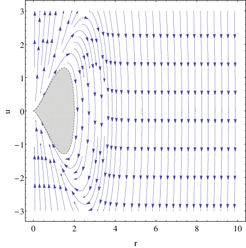
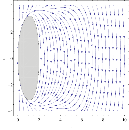
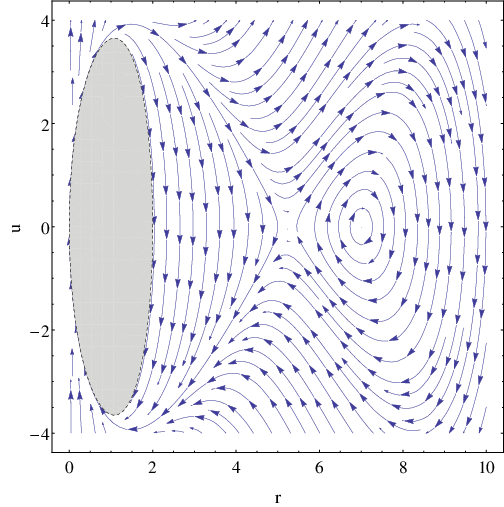
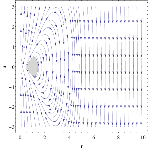
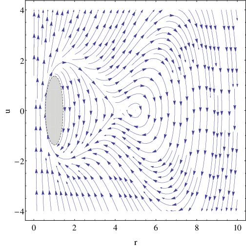
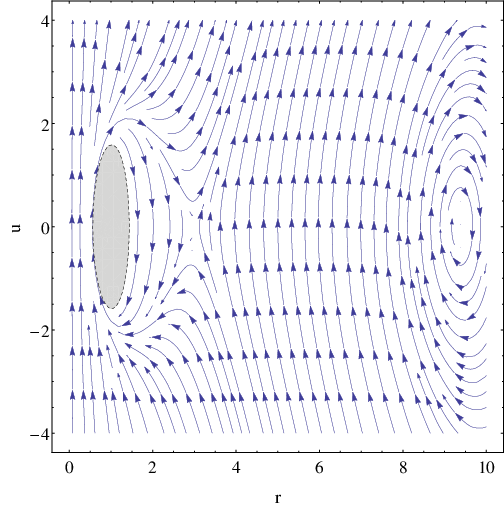
Figure 10: Phase space for mass particles with $L=0$, $L=3M$, $L=3.5M$ (from left to right) and with $Q=0$ (upper row) y $Q=0.9M$ (lower row). The dark zone correspond to the forbidden region given by $\epsilon<\frac{\mu}{2}$.

When $\mu=1$ the dynamical system takes the form

$$r^{\prime} =ru,$$

$$u^{\prime} =r\left(r\left(L^{2}-Mr+Q^{2}\right)-3L^{2}M\right)+2\left(L^{2}Q^{2}+u^{2}\right),$$

with phase spaces displayed for different values of $L$ and $Q$ in Fig. 10. The portraits show very clearly the repulsive nature of the singularity discussed above. The fixed points lie on the line $u=0$ and are given by the roots of

$$r^{3}M-r^{2}\left(L^{2}+Q^{2}\right)+3rL^{2}M-2L^{2}Q^{2}=0.$$

The root structure of this polynomial is not uniform in the parameters $\{M,Q,L\}$. Let us concentrate for definiteness in the most interesting case $L\neq 0$ and $0<|Q|<M$. It turns out that this equation always has one real solution which lies inside the excluded region and corresponds to a hyperbolic critical point that happens to be a center (purely imaginary eigenvalues). Moreover, there exists $L_{0}(M,Q)>0$ such that, for $0<|L|\leq L_{0}$ this is the only root. For $|L|=L_{0}$, there is second root which is double (and hence a non-hyperbolic fixed point for the dynamical system). For $|L|>L_{0}$ there are two additional hyperbolic points, both lying outside the excluded region to its right. The one closer to the excluded region is a saddle and the one with largest value of $r$ is a center. The function $L_{0}(M,Q)$ is defined as the only positive and real solution of

$$L^{6}\left(8Q^{2}-9M^{2}\right)+6L^{4}\left(18M^{4}-21M^{2}Q^{2}+4Q^{4}\right)+3L^{2}\left(8Q^{6}-3M^{2}Q^{4}\right)+8Q^{8}=0.$$

Existence of a unique positive solution of this equation is guaranteed for $0<|Q|<M$. The function $L_{0}(Q,M)$ is displayed in Fig. 11, note that $L_{0}(Q=0)=2\sqrt{3}M$. These points are analogous to the well-known critical points in the Schwarzschild spacetime and of course they coincide in the limit $Q=0$.

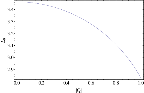
Figure 11: The image shows the variation of the function $L_{0}$ with respect to the value of $Q$. The plot is given in units where $M=1$.

7 Conclusions

The main result of this work is a dynamical systems method of analyzing causal geodesics in stationary and spherically symmetric Kerr-Schild spacetimes. A remarkable result is that the geodesics can be globally described as the motion of a Newtonian particle in the presence of a radial potential. For spacetimes with singularities at the center we have developed a generalization of the MacGehee transformation that allows for a regularization of the origin and hence for a description of the approach to the singularity in terms of regular variables. In particular, the dynamics at the collision manifold can be analyzed, which gives us useful information for the physical trajectories. We have applied this method to the Schwarzschild and Reissner-Nordström spacetimes. Besides the regularized analysis of the singularity in these spacetimes, we have emphasized the importance of the presence of excluded regions, which in effect makes the phase space diagram acquire a non-trivial topology. This topology and the property that the phase space portrait is independent of whether we deal with an advanced or a retarded Kerr-Schild patch allows one to study in the geodesic motion is spacetimes with complicated global behavior (e.g. the Reissner-Nordström spacetime) in terms of a single two-dimensional phase space portrait.

Appendix A Absence of Mcgehee transformation decoupling the system in $(u,v)$

In this appendix we prove a no-go Theorem for McGehee-type transformations capable of decoupling the dynamic equations of a point particle on a plane under the influence of a general radial potential $V(|x|)$. Specifically, we intend to analyze the dynamical system

$$\dot{x} =y$$

$$\dot{y} =-\nabla V(|x|)=\Lambda(|x|)x.$$ (69)

where $\{x,y\}$ are coordinates on an open subset of ${\cal N}$ of $\mathbb{C}^{2}$ and $\nabla=\partial_{x^{1}}+i\partial_{x^{2}}$. In view of the transformation proposed by McGehee for the power-law potential (39), we define the generalized MacGehee transformation

$$x =e^{i\theta}\xi_{1}(r),$$

$$y =e^{i\theta}\xi_{2}(r)(u+iv),$$ (70)

$$d\tau =\xi_{3}(r(s))ds,$$

where $\xi_{1},\xi_{2},\xi_{3}:\mathbb{R}^{+}\to\mathbb{R}$ are smooth and non-zero functions to be determined. Note that $\xi_{1}(r)$ must be invertible for this transformation to be well-defined. The new coordinates $\{u,v,r,\theta\}$ take values on $\mathbb{R}$ (for $u,v$), in $\mathbb{R}^{+}$ (for $r$) and on $S^{1}$ (for $\theta$). We note that making $\xi_{1}$ complex does not define a more general transformation since it can be reduced to the above one by redefining the variable $\theta$. Given that we are replacing the power-law potential $V(|x|)=|x|^{-\sigma}$ by a general radial potential, it is reasonable to keep the general structure of the original McGehee transformation and introduce general functions of $r$ in the transformation. In this sense, we can consider (70) as the most general Mcgehee transformation in this context. We prove the following result

Lemma 16.

Except for potentials which are either power-law ($V(r)=Cr^{-\sigma}$) or logarithmic ($V(r)=C\mbox{ln}\,r$) there exists no generalized McGehee transformation capable of decoupling the system (69) in the coordinates $(u,v)$.

Proof. In the new parameter $s$, the dynamical system is

$$x^{\prime} =\xi_{3}(r)y$$

$$y^{\prime} =\xi_{3}(r)\Lambda(|x|)x,$$

where prime is derivative with respect to $s$. Inserting the transformation (70) yields

$$i\theta^{\prime}\xi_{1}+\frac{d\xi_{1}}{dr}r^{\prime}=\xi_{2}\xi_{3}(u+iv),$$

$$\left(i\theta^{\prime}\xi_{2}+\frac{d\xi_{2}}{dr}r^{\prime}\right)\left(u+iv\right)+\xi_{2}(u^{\prime}+iv^{\prime})=\Lambda(\xi_{2})\xi_{1}\xi_{3}.$$

Taking real and imaginary parts in the first equation determines $r^{\prime}$ and $\theta^{\prime}$ as

$$r^{\prime}=\frac{u\xi_{2}\xi_{3}}{d\xi_{1}/dr},$$

$$\theta^{\prime}=\frac{v\xi_{2}\xi_{3}}{d\xi_{1}/dr}.$$ (71)

Substituting into the second equation and separating real and imaginary parts gives

$$v^{\prime} =-uv\,\xi_{3}(r)\left(\frac{d\xi_{2}/dr}{d\xi_{1}/dr}+\frac{\xi_{2}}{\xi_{1}}\right),$$

$$u^{\prime} =\xi_{3}(r)\left(-\frac{u^{2}d\xi_{2}/dr}{d\xi_{1}/dr}+\frac{v^{2}\xi_{2}(r)}{\xi_{1}(r)}\right)+\xi_{3}(r)\frac{\xi_{1}(r)\Lambda(\xi_{1}(r))}{\xi_{2}(r)}.$$ (72)

To uncouple the system in $(u,v)$ it is necessary that no function of $r$ appears in the equations for $(u^{\prime},v^{\prime})$. From the equation for $u^{\prime}$, we need to impose

$$\xi_{3}(r)\left(\frac{d\xi_{2}/dr}{d\xi_{1}/dr}\right) =\beta\alpha$$

$$\frac{\xi_{3}(r)\xi_{2}(r)}{\xi_{1}(r)} =\alpha,$$ (73)

where $\alpha,\beta$ are constants with $\alpha\neq 0$. The second one fixes $\xi_{3}$ as

$$\xi_{3}(r)=\frac{\alpha\xi_{1}(r)}{\xi_{2}(r)},$$

which inserted into the first one gives

$$\frac{\xi_{1}(r)d\xi_{2}/dr}{\xi_{2}(r)d\xi_{1}/dr}=\beta$$

This equation can be integrated to obtain:

$$\xi_{2}(r)=c\,\xi_{1}(r)^{\beta}.$$ (74)

where $c\neq 0$ is a constant. Inserting these expressions into (71)-(72) the dynamical system becomes

$$r^{\prime} =\alpha u\frac{\xi_{1}}{d\xi_{1}/dr}$$

$$\theta^{\prime} =\alpha v$$

$$v^{\prime} =-\alpha(1+\beta)uv$$ (75)

$$u^{\prime} =\frac{\alpha}{c^{2}}\xi_{1}(r)^{2(1-\beta)}\Lambda(\xi_{1}(r))+\alpha\left(v^{2}-\beta u^{2}\right).$$

From the expression for $u^{\prime}$, the system is uncoupled if and only if

$$\xi_{1}(r)^{2(1-\beta)}\Lambda(\xi_{1}(r))=\alpha_{3}$$

for some constant $\alpha_{3}$, i.e. $\Lambda(r)$ is a power-law. Since the potential $V$ is related to $\Lambda$ by

$$\frac{dV}{dr}=-\Lambda(r)r$$

it follows that the only case for which the generalized McGehee transformation decouples the system is when the potential itself is a power-law or logarithmic (recall that an additive constant is completely irrelevant in the potential $V$). $\blacksquare$

References

- [Anabalón et al., 2009] Anabalón, A., Deruelle, N., Morisawa, Y., Oliva, J., Sasaki, M., Tempo, D., and Troncoso, R. (2009). Kerr–Schild ansatz in Einstein–Gauss–Bonnet gravity: an exact vacuum solution in five dimensions. Classical and Quantum Gravity, 26(6):065002.
- [Anabalón et al., 2011] Anabalón, A., Deruelle, N., Tempo, D., and Troncoso, R. (2011). Remarks on the Myers-Perry and Einstein–Gauss–Bonnet rotating solutions. International Journal of Modern Physics D, 20(05):639–647.
- [Belbruno and Pretorius, 2011] Belbruno, E. and Pretorius, F. (2011). A dynamical system’s approach to Schwarzschild null geodesics. Classical and Quantum Gravity, 28(19):195007.
- [de Moura and Letelier, 2000] de Moura, A. P. and Letelier, P. S. (2000). Chaos and fractals in geodesic motions around a nonrotating black hole with halos. Physical Review E, 61(6):6506.
- [Eddington, 1924] Eddington, A. S. (1924). A comparison of Whitehead’s and Einstein’s formulae. Nature, 113:192.
- [Finkelstein, 1958] Finkelstein, D. (1958). Past-future asymmetry of the gravitational field of a point particle. Physical Review, 110(4):965.
- [Gibbons et al., 2005] Gibbons, G. W., Lü, H., Page, D. N., and Pope, C. (2005). The general Kerr–de Sitter metrics in all dimensions. Journal of Geometry and Physics, 53(1):49–73.
- [Hackmann et al., 2008] Hackmann, E., Kagramanova, V., Kunz, J., and Lämmerzahl, C. (2008). Analytic solutions of the geodesic equation in higher dimensional static spherically symmetric spacetimes. Physical Review D, 78(12):124018.
- [Kerr and Schild, 1965] Kerr, R. P. and Schild, A. (1965). A new class of vacuum solutions of the Einstein field equations. Atti del Congregno Sulla Relativita Generale: Galileo Centenario.
- [Levin, 2000] Levin, J. (2000). Gravity waves, chaos, and spinning compact binaries. Physical review letters, 84(16):3515.
- [Levin and Perez-Giz, 2008] Levin, J. and Perez-Giz, G. (2008). A periodic table for black hole orbits. Physical Review D, 77(10):103005.
- [Levin and Perez-Giz, 2009] Levin, J. and Perez-Giz, G. (2009). Homoclinic orbits around spinning black holes. I. Exact solution for the Kerr separatrix. Physical Review D, 79(12):124013.
- [Málek, 2012] Málek, T. (2012). Exact solutions of general relativity and quadratic gravity in arbitrary dimension. arXiv preprint arXiv:1204.0291.
- [McGehee, 1981] McGehee, R. (1981). Double collisions for a classical particle system with nongravitational interactions. Commentarii Mathematici Helvetici, 56(1):524–557.
- [Misra and Levin, 2010] Misra, V. and Levin, J. (2010). Rational orbits around charged black holes. Physical Review D, 82(8):083001.
- [Moeckel, 1992] Moeckel, R. (1992). A nonintegrable model in general relativity. Communications in Mathematical Physics, 150(2):415–430.
- [Myers and Perry, 1986] Myers, R. C. and Perry, M. (1986). Black holes in higher dimensional space-times. Annals of Physics, 172(2):304–347.
- [Nordström, 1918] Nordström, G. (1918). On the energy of the Gravitation field in Einstein’s Theory. Koninklijke Nederlandse Akademie van Weteschappen Proceedings Series B Physical Sciences, 20:1238–1245.
- [Parry, 2012] Parry, A. R. (2012). A survey of spherically symmetric spacetimes. arXiv preprint arXiv:1210.5269.
- [Perez-Giz and Levin, 2009] Perez-Giz, G. and Levin, J. (2009). Homoclinic orbits around spinning black holes. II. The phase space portrait. Physical Review D, 79(12):124014.
- [Pugliese et al., 2011a] Pugliese, D., Quevedo, H., and Ruffini, R. (2011a). Circular motion of neutral test particles in Reissner-Nordström spacetime. Physical Review D, 83(2):024021.
- [Pugliese et al., 2011b] Pugliese, D., Quevedo, H., and Ruffini, R. (2011b). Motion of charged test particles in Reissner-Nordström spacetime. Physical Review D, 83(10):104052.
- [Reissner, 1916] Reissner, H. (1916). Über die eigengravitation des elektrischen Feldes nach der Einsteinschen Theorie. Annalen der Physik, 355(9):106–120.
- [Stoica and Mioc, 1997] Stoica, C. and Mioc, V. (1997). The Schwarzschild problem in astrophysics. Astrophysics and Space Science, 249(1):161–173.
- [Suzuki and Maeda, 1999] Suzuki, S. and Maeda, K.-i. (1999). Signature of chaos in gravitational waves from a spinning particle. Physical Review D, 61(2):024005.