Localization transition, Lifschitz tails and rare-region effects in network models

Abstract

Effects of heterogeneity in the suspected-infected-susceptible model on networks are investigated using quenched mean-field theory. The emergence of localization is described by the distributions of the inverse participation ratio and compared with the rare-region effects appearing in simulations and in the Lifschitz tails. The latter, in the linear approximation, is related to the spectral density of the Laplacian matrix and to the time dependent order parameter. I show that these approximations indicate correctly Griffiths Phases both on regular one-dimensional lattices and on small world networks exhibiting purely topological disorder. I discuss the localization transition that occurs on scale-free networks at $\gamma=3$ degree exponent.

I Introduction

Epidemic spreading in complex networks such as biological populations and computer networks is of great interest, both for practical applications and from a fundamental point of view ABR02 ; DFR02 ; NR10 . Simple models, like the Contact Process (CP) Harris (1974a); Liggett (1985) has been introduced and studied intensively by various techniques. They can also be considered as simple models of information spreading in social pv04 or in brain networks MMNat . In these models sites can be infected (active) or susceptible (inactive). Infected sites propagate the epidemic to all of their neighbors, with rate $\lambda$, or recover (spontaneously deactivate) with rate $\nu=1$. The susceptible-infected-susceptible (SIS) SIS model differs slightly from the CP, in which the branching rate is normalized by $k$, the number of outgoing edges of a vertex permitting an analytic treatment via symmetric matrices. By decreasing the infection (communication) rate of the neighbors a continuous phase transition may occur at some $\lambda_{c}$ critical point from a steady state with finite activity density $\rho$ to an inactive one, with $\rho=0$. The latter is also called absorbing, since no spontaneous activation of sites is allowed. In case of the SIS $\lambda_{c}=0$ in networks with a degree distribution decaying slower than an exponential BCS13 . The transition type is continuous and belongs to the directed percolation universality class Marro and Dickman (1999); rmp ; Ódor (2008); HH .

In real systems various heterogeneities occur, that may cause deviations from the results of the homogeneous models. From the homogeneous system point of view if the disorder varies rapidly both in space and time, its contribution can be described by an increased temperature or noise of the system Ódor (2008). In the quasi-static limit, when the variation of the heterogeneity is much slower the dynamics of the pure model we can consider it as a quenched disorder. It causes a memory effect, whose relevancy has been studied in quantum and nonequilibrium systems (see Vojta (2006)).

In networks, with finite topological dimension, defined as $N\propto r^{D}$, where $N$ is the number of nodes within the (chemical) distance $r$, it was shown Muñoz et al. (2010), that disorder can be relevant. Heterogeneities can induce arbitrarily large, rare-regions (RR), changing their state exponentially slowly as the function of their sizes, induce so called Griffiths Phases (GP) Griffiths (1969); Vojta (2006). In these phases the dynamics is slow and non-universal and at the phase transition point it is even slower, logarithmic dynamical scaling may occur. These heterogeneities can be explicit features of the interactions or maybe the result of the topology of the graph.

Recent observations show generically slow time evolution in various system. For example in the working memory of the brain Johnson or in recovery processes following virus pandemics pv04 ; PV01 ; KK11 power-law type of time dependencies have been found, resembling of dynamical critical phenomena Chialvo . In social networks the occurrence of generic slow dynamics was suggested to be the result of the non-Markovian, bursty behavior of agents in small world networks KK11 . Very recently it has been shown burstcikk , that bursty dynamics can arise naturally, in network models as the consequence of power-law decaying auto-correlations due to the collective behavior of Markovian variables.

Disorder effects are stronger in quantum systems, where the thermal noise does not fade effects of the quenched noise. However, in several cases the critical behavior is dictated by an infinitely strong disorder fixed point, resulting in robust universality classes, that can be observed even in classical models. In particular, the same universal behavior occurs in disordered quantum Ising chains and the CP IMrev . The dynamics of the CP far in the absorbing state, can be mapped to the quantum-mechanical one, described by the disordered Hamiltonian of the Anderson type (see KK93 ).

Heterogeneous Mean Field (HMF) theory provides a good approximation in network models, when the fluctuations are irrelevant Boguñá et al. (2009); FCP12 ; Fer14 . To describe quenched disorder in networks the so-called Quenched Mean-Field (QMF) approximation is introduced CWW08 ; Mieg09 ; CP10 ; GDOM12 and heterogeneities of the steady state are quantified by calculating the Inverse Participation Ratio (IPR) of the principal eigenvector of the adjacency matrix. Effects of the quenched disorder on the dynamical behavior of SIS have recently been compared using QMF approximations in different network models. Numerical evidences have been provided for the relation of localization to RR effects, that slows the dynamics wbacikk ; basiscikk .

The success of this relation is the consequence of the fact that GP effects arise even in the active phase, where localization of the steady state can be traced by the IPR value. Although for best understanding the effects of dynamical fluctuations should also be taken into account, such approaches, like renormalization group methods (RG) Monthus ; KI11 ; JK13 have some limitations. For example, strong disorder RG works around an infinite disorder fixed point, which is not always present, still Griffiths singularities can co-exist with the clean critical behavior HoyosVojta . Furthermore, this method cannot handle models with pure topological inhomogeneity.

In this work I show that the QMF theory describes localization in the one-dimensional SIS model, with quenched disorder, in agreement with the expectation that RR effects and GP should occur below the critical point. I extend previous localization studies by considering distributions of the IPR and eigenvalues, casting more light on the localization transition of SIS in various complex networks. In particular, I investigate SIS on scale-free (SF) networks, possessing $P(k)\propto k^{-\gamma}$ degree distributions and provide numerical evidence for a localization transition at $\gamma=3$.

Very recently Moretti and Muñoz MMNat have investigated hierarchical, brain networks by simulations and QMF approximations. They gave a brief overview about the relation of slow dynamics and Lifschitz tails in synchronization and spreading models Matj . Lifschitz tails have provided valuable information in regular, equilibrium systems about the Griffiths singularities (see for example Nus91 ). In network models they have been studied in mathematics literature mainly KKM . In graph theory there is a growing interest in spectral properties of linear operators, mostly of the adjacency matrix or the graph Laplacian (see for example Chung ; Miegbook ). In physics literature Samukhin et al. SDM08 provided analytical forms for the Laplacian spectrum of complex random networks and for the dynamical two-point functions of random walks running on them. They pointed out that the minimum degree of vertexes, is important for the dynamics, which is related to the lower edge of the Laplacian. On the other hand numerical evidences have been shown that the spectral gaps at the lower edge describe well the slow-down of dynamics due to disorder in models like the CP TLNG05 or by synchronization transition BC ; DNM06 . This is based on the validity of linearization near the phase transition point. In this case the probability distribution at the lower tail of the Laplacian can be considered the density of states, the Lifschitz tail of the disordered network model. If it holds it enables us to describe the dynamics near the critical point. In this study I calculate the lower tail distributions of the Laplacian of the networks considered and test how well does it describe the GP behavior of the SIS.

II Summary of earlier studies: localization versus RR effects

Starting from the master equation for state vectors of site occupancies, $|P_{(n_{1},n_{2},...,n_{N})}(t)\rangle$ where $n_{i}=0$ or $1$, one can derive the QMF theory for the SIS model Mieg09 ; GDOM12 . Although QMF neglects the dynamical correlations, it can take into account heterogeneities of the network by considering the vector of infection probabilities $\rho_{i}(t)$ of node $i$ at time $t$

$$\frac{d\rho_{i}(t)}{dt}=-\rho_{i}(t)+\lambda(1-\rho_{i}(t))\sum_{j=1}^{N}A_{ij}w_{ij}\rho_{j}(t)~{}.$$ (1)

Here $A_{ij}$ is an element of the adjacency matrix and $w_{ij}$ describes the possibility of weights attributed to the edges. For large times the SIS model evolves into a steady state, with an order parameter $\rho\equiv\langle{\rho_{i}}\rangle$. This equation with $i\leftrightarrow j$ symmetric weights can be treated by a spectral decomposition on an orthonormal eigenvector basis. Furthermore the non-negativity of the $B_{ij}\equiv A_{ij}w_{ij}$ matrix involves a unique, real, non-negative largest eigenvalue $y_{M}$.

For $t\rightarrow\infty$ the system evolves into a steady state and the infection probabilities can be expressed via $B_{ij}$ as

$$\rho_{i}=\frac{\lambda\sum_{j}B_{ij}\rho_{j}}{1+\lambda\sum_{j}B_{ij}\rho_{j}}\ .$$ (2)

The order parameter (prevalence) $\rho\equiv\langle{\rho_{i}}\rangle$ becomes finite above an epidemic threshold $\lambda_{c}$. In the QMF approximation one finds $\lambda_{c}$ and $\rho(\lambda)$ around it from the principal eigenvector. Using a Taylor expansion of $\rho$ one can solve Eq. (2) and find that the threshold is related to the largest eigenvalue of $B_{ij}$ as: $1/\lambda_{c}=y_{M}$. The order parameter near, above $\lambda_{c}$ can be approximated via

$$\rho(\lambda)\approx a_{1}\Delta+a_{2}\Delta^{2}+...\ ,$$ (3)

where $\Delta=\lambda y_{M}{-}1{\ll}1$ and the coefficients

$$a_{j}=\sum_{i=1}^{N}e_{i}(y_{j})/[N\sum_{i=1}^{N}e_{i}^{3}(y_{j})]\,$$ (4)

are functions of eigenvectors ${\bf e}(y_{j})$ of the largest eigenvalues ($j=M,M-1,M-2,...$) of $B_{ij}$. This expression is exact, if there is a gap between $y_{M}$ and $y_{M-1}$ Mieg12 .

It was proposed in GDOM12 and tested on weighted Barabasi-Albert models wbacikk that the localization of activity in the active steady state can be characterized by the $IPR$ value, related to the eigenvector of the largest eigenvalue $\mbox{\boldmath$e$}(y_{M})$ as

$$I(N)\equiv\sum_{i=1}^{N}e_{i}^{4}(y_{M})$$ (5)

This quantity disappears as $\sim 1/N$ in case of homogeneous eigenvector components or remains finite if the activity is concentrated on a finite number of nodes.

III Lifschitz tails in network models

Besides IPR calculation, that works in the active steady state, some other way to check RR effects would be desirable. The study the spectrum tail of the Laplacian will be introduced here in the hope of providing information about GPs below the critical point of the SIS. The Laplacian matrix of a graph is defined as

$$L_{ij}=\delta_{ij}\sum_{l}A_{jl}-A_{ij}\ ,$$ (6)

which takes values $-1$ for pairs of connected vertexes and the degree $k_{i}$ in the diagonal. The Laplacian is positive-semi-definite, i.e.: $\Lambda_{i}\geq 0$ and $\Lambda_{1}=0$. The smallest non-zero eigenvalue $\Lambda_{2}$ is called the spectral gap.

Near the critical point, in the inactive phase we can linearize the dynamical equation of SIS (1) as

$$\frac{d\rho_{i}(t)}{dt}=-\rho_{i}(t)+\lambda\sum_{j}B_{ij}\rho_{j}(t)\ .$$ (7)

We can rewrite it, using the weighted (symmetric) Laplacian matrix MO08 ; M11

$$L_{ij}=\delta_{ij}\sum_{l}B_{jl}-B_{ij}\ ,$$ (8)

which has the sums of weights in the diagonal, expressed by the Kronecker delta ($\delta_{ij}$), as follows

$$\frac{d\rho_{i}(t)}{dt}=\left[\lambda\delta_{ij}\sum_{l}B_{jl}-1\right]\rho_{i}(t)-\lambda\sum_{j}L_{ij}\rho_{j}(t)\ .$$ (9)

A linear stability analysis can be performed above the critical point, similarly to the synchronization process BC . For the normal modes of the perturbations above the absorbing state we can write

$$\frac{d\rho_{i}(t)}{dt}=-\lambda\sum_{j}L_{ij}\rho_{j}(t)\ .$$ (10)

By this approximation we replaced the diagonal elements in Eq. (7), from $-1$ to $-\lambda L_{ii}$, which increases the spontaneous recovery rate $\nu$ of sites, pushing the system deeper into the inactive phase. In spreading models it is known that the value of $\nu$ can modify non-universal quantities, shift $\lambda_{c}$, but in the inactive phase, where this approach is applied, it is not expected to induce relevant RR effects, it can make them weaker and harder to detect. However, I have confirmed this approximation in case of CP on networks with purely topological disorder.

Using the spectrum of $L_{ij}$ one can make the eigenvalue expansion

$$\rho_{i}(t)=\sum_{jl}e^{-\lambda\Lambda_{l}t}f_{i}(\Lambda_{l})f_{j}(\Lambda_{l})\rho_{j}(0)\ ,$$ (11)

where $f_{i}(\Lambda_{l})$ is $i$-th the component of the $l$-th eigenvector of the Laplacian. The total density is determined by the lowest eigenvalues of the spectrum

$$\rho(t)\sim\sum_{l=2}^{N}e^{-\lambda\Lambda_{l}t}$$ (12)

for any network. In finite systems there is always a finite $\Lambda_{2}>0$ gap, causing exponential cutoff in the decay of the order parameter. In this study I consider $P(\Lambda)$ above $\Lambda_{2}$, i.e. shift the numerically obtained distributions to zero and express $\rho(t)$ as the Laplace transform of $P(\Lambda$) in the continuum limit

$$\rho(t)\propto\int_{\Lambda_{2}}^{\Lambda_{M}}d\Lambda\ P(\Lambda)e^{-\lambda\Lambda t}\ ,$$ (13)

where $\Lambda_{M}$ corresponds to the experimentally determined end of tail value of the finite network. Note, that the control parameter $\lambda$ appears as a constant, which can induce non-universal power-laws in the inactive GP.

One can also take into account the original diagonal elements of (7), if one considers the CP instead of SIS, where the interactions are normalized by the degree as $\lambda_{i}/k_{i}$. In case of purely topological heterogeneities the linearized, governing equation takes the form:

$$\frac{d\rho_{i}(t)}{dt}=-\rho_{i}(t)+\sum_{j=1}^{N}\frac{\lambda}{k_{j}}A_{ij}\rho_{j}(t)\ .$$ (14)

thus the sum of non-diagonal elements: $\frac{\lambda}{k_{j}}A_{ij}$ is constant: $\lambda$. The eigenvalue spectrum of the matrix $L^{\prime}_{ij}=\delta_{ij}-\frac{\lambda}{k_{j}}A_{ij}$ is the linear combination of the normalized Laplacian: $L^{\prime}_{ij}=\frac{\lambda}{k_{j}}L_{ij}-\delta_{ij}(\lambda-1)$ for such models. Therefore, by performing a spectral analysis of $L^{\prime}_{ij}$ we can investigate the lower gap behavior. The penalty is that we have non-symmetric matrices, which can be diagonalized by slower algorithms. I have determined this spectrum for uncorrelated random and generalized small networks (for definition see later sections) and found tails very similar as that of SIS, except from the linear transformation.

For comparison I calculated the Laplacian eigenvalue spectrum of the Erdős Rényi (ER) ER graph with $N=10^{4}$ nodes and $\langle k\rangle=4$ average degree. Averaging over $2.5\times 10^{5}$ random graph realizations and histogramming, with the bin size $\delta\Lambda=0.001$ one can determine numerically the probability distribution $P(\Lambda_{i})$ in the region $0<\Lambda<0.6$. The gap size due to the finite system was $\Lambda_{2}=0.036$, that I subtracted: $\Delta\Lambda_{i}=\Lambda_{i}-\Lambda_{2}$. A good fitting can be obtained with the cumulative distribution derived form SDM08 with the numerical factors shown in Fig. 1.

$$P(\Delta\Lambda)\simeq\Delta\Lambda^{1/10}e^{-a/\sqrt{\Delta\Lambda}}\ .$$ (15)

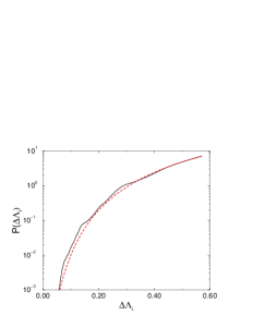
Figure 1: (Color online) Lifschitz tail of the ER graph with $\langle k\rangle=4$ and $N=10^{4}$. The dashed line shows a numerical fit with the form (15) as: $2400\Delta\Lambda_{i}^{1/10}\exp(-4.5/(\Delta\Lambda_{i}^{1/2}).$

The Laplace transform of (15) predicts the long time asymptotic behavior of the density decay

$$\rho(t)\sim e^{-(ct\lambda)^{1/3}}$$ (16)

which is a $\lambda$ dependent stretched exponential time dependence. Numerical simulations of the disordered CP on ER graphs have obtained indeed $\lambda$ dependent stretched exponential density decay behavior below the critical point GPCNlong . However, the validity of Eq. (15) is limited to $t^{1/3}/\ln N<<1$ SDM08 , hence in numerically accessible systems this should be observable for very short times only. In density decay simulations of SIS on pure ER systems with $N=5\times 10^{6}$ the effect of topological disorder can be seen for very early times, otherwise exponential decay is observed.

Contrary, for a power-law distributed $P(\Lambda)$ the Laplace transformation results in a power-law decaying density

$$\rho(t)\propto\int_{\Lambda_{2}}^{\Lambda_{M}}d\Lambda\ \Lambda^{x}e^{-\lambda\Lambda t}\propto t^{-\lambda(x+1)}\ ,$$ (17)

which suggests a GP behavior for the model. Therefore, in the following sections I determine numerically $P(\Lambda)$ for certain models and determine how well can the tail behavior be fitted by a power-law form. By knowing dynamical simulation results about the existence of GPs in these systems I test the predicting power of this approach. Later, I apply the method to more difficult cases and try to support statements about existence of GPs in them.

IV QMF of the one-dimensional SIS model with quenched infection rates

The CP on regular lattices with quenched infection rates has been studied by many authors (for a recent overview see Vojta (2006)). First Noest showed, using the Harris criterion Harris (1974a), that spatially quenched disorder (frozen in space) changes the critical behavior of the directed percolation for $D<4$. Field theoretical RG Janssen97b found quenched disorder to be a marginal perturbation below $D<4$ and the stable fixed point shifted to an unphysical region. This means that spatially quenched disorder changes the critical behavior of the directed percolation. This conclusion is supported by simulation results MoreiraDickman96 ; MF08 ; TFM09 . In the sub-critical region they found GP, in which the time dependence is governed by non-universal power-laws, while in the active phase the relaxation of activity survival is algebraic. A real-space RG study by HIV02 showed that in case of strong enough disorder the critical behavior is controlled by the infinite randomness fixed point and below $\lambda_{c}$ GP behavior emerges. Very recently GP is reported in the five dimensional CP below the clean, mean-field critical point HoyosVojta .

Here I consider the one-dimensional SIS model with quenched disorder (QSIS), which exhibits $i\leftrightarrow j$ symmetry in the governing Eq. (1). First I investigated the case of uniformly distributed disorder, by putting symmetric weights, drawn from the distribution $w_{i,i+1}\in(0,1)$, on the edges connecting neighbors.

The spectral analysis was done using the sparse matrix functions of the software package OCTAVE OCT . The largest eigenvalues and eigenvectors were determined and averaged over thousands of disorder realizations for $N=10^{3},...,5\times 10^{5}$. The probability distribution of (5): $P(I(N))$ is calculated by histogramming with the bin size: $\delta I=0.001$. As one can see on Figure 2 the mean values of IPR remain finite and localization persists for any size. The $P(I(N))$ distributions do not smear, but shift to slower values by increasing the size. In the $N\to\infty$ limit one can extrapolate the mean values ${\bar{P}(I(N))}$ with a power-law, resulting in the asymptotic value $I=0.168(2)$.

The case of bimodal disorder distribution, where a fraction $q$ take a reduced value $r\lambda$, while the remaining fraction of the nodes take a value $(1-r)\lambda$:

$$p(\lambda_{i})=(1-q)\delta[\lambda_{i}-(1-r)\lambda]+q\delta(\lambda_{i}-r\lambda)\$$ (18)

has also been studied. For $q=0.5$ only slow convergence of $I(N)$ could be observed, so I used a strong disorder distribution: $p=0.1$ and $r=0.9$. In this case the IPR values are larger than for uniform distribution but extrapolate roughly to the same $I=0.125(15)$ value in the thermodynamic limit.

The finite size scaling of the largest eigenvalue determines the critical point within the QMF approximation $\lambda_{c}=1/y_{M}$. This extrapolates with a similar correction to scaling as for $I(N)$ to the value $\lambda_{c}=0.548+(0.35/N)^{0.27}$. Naturally, this value is much smaller than the true critical point of the model due to the nature of approximations made.

Figure 2: (Color online) Finite size scaling of the IPR results of the one-dimensional QSIS model. Mean values of IPR for uniformly (bullets) and binary (squares) distributed disorder. Dashed line shows an extrapolation to $N\to\infty$ as: $0.13(1)+(0.17/N)^{0.1}$. Dotted line: $0.12(1)+(0.54/N)^{0.15}$. Inset: distributions of $I(N)$ in case of uniform distributed disorder for various sizes.

Thus the IPR, defined in the supercritical phase, predicts a localization in agreement with the known RR effects of CP in one-dimension. Note, that for left-right asymmetric disorder, when sites interact with their right or left neighbors, the localization disappears in the $N\to\infty$ limit in agreement with the recent results Robiuj .

For the QSIS model the lower tail of the Laplacian has been determined numerically for $N=2\times 10^{4}$ . As Fig. 3 shows one can fit the tails with power-laws well. For uniform distribution

$$P(\Lambda)\sim\Lambda^{4.75}\ ,$$ (19)

suggesting a GP behavior with decay law

$$\rho(t)\propto t^{-5.75\lambda}$$ (20)

similarly for the known result of the CP.

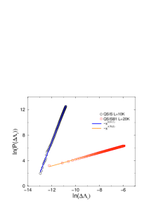
Figure 3: (Color online) Lifschitz tails in 1D QSIS models. Squares: tail distribution of the $N=2\times 10^{4}$ QSIS with bimodal random infection rates. Circles: tail distribution of the $L=10^{4}$ QSIS with uniform random distribution of infection rates. This curve is shifted by $\ln(10)$ both in $x$ and $y$ direction for better visibility. Solid line shows a power-law fit $\sim\ln(\Delta\Lambda_{i})^{4.75(5)}$, dotted line : power-law fit $\sim\ln(\Delta\Lambda_{i})^{0.51(1)}$.

In conclusion I demonstrated here that even for this low dimensional model, where dynamical fluctuations are relevant at the critical point the effect of quenched disorder away from $\lambda_{c}$ can be well described via the QMF approximation.

V Localization transition on a generalized small world network model

In this section I show results of the QMF analysis done on networks, which exhibit purely topological disorder. I analyzed a generalized small-world (GSW) network model an ; kleinberg ; BB ; Juhasz ; Juhasz3 , which exhibits finite $D$, defined as follows. We add to a one-dimensional lattice (a ring) a set of long-range edges of arbitrary, unbounded, length. The probability that a pair of sites separated by the Euclidean distance $l$ is connected by an edge decays with $l$ as

$$P(l)\simeq\beta l^{-s}$$ (21)

for large $l$ and amplitude $\beta$. These networks interpolate between the quasi-one-dimensional network ($s=\infty$) and the mean-field limit ($s=0$). Recently, simulations of the CP provided numerical evidence for the emergence of GP in $s\geq 2$ networks GPCNlong . When a quenched disorder added to the birth process rates a recent RG study arrived to similar conclusions JK13 .

Here I show the finite size scaling results of $\langle I(N)\rangle$ defined on these GSW networks for sizes $N=10^{3},...2\times 10^{5}$. As Fig. 4 shows a clear localization occurs in the $s=2$ case with $\beta=0.1$ for $N\to\infty$. For $s=2$ and large $\beta$, where the CP simulations and the RG analysis were not completely conclusive, a slow crossover to localization can be concluded using an extrapolation to the data points: $I(N)=0.20(2)-0.18(1/N)^{0.02}$ (see inset of Fig. 4). Here, the unusually small crossover exponent expresses the very slow change from small to large IPR in the infinite size limit.

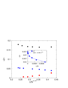
Figure 4: (Color online) Mean values of IPR of the SIS model on GSW networks. For $s=2$, $\beta=0.1$ (diamonds) extrapolation to $N\to\infty$ shows the localization of the principal eigenvector. For $s=1$, $\beta=0.1$ (bullets) one observes a homogeneous steady state in the thermodynamic limit. For $s=2$, $\beta=3$ (squares) a slow crossover to localization seems to emerge. On the main plot abscissa is rescaled to allow better visibility of the finite size scaling. Inset: The crossover region magnified, rescaled and fitted with a power-law.

This result suggests that the GP of the SIS model may exist for any $\beta$ in case of marginal ($s=2$) GSW networks. In numerical simulations one should observe GP regions of shrinking size, becoming invisible for large $\beta$-s. Finally, for $s=1$ one observes a homogeneous steady state above the critical point.

The $L_{ij}$ matrices have also been diagonalized for $N\leq 4\times 10^{4}$ in case of $s=1$ and $s=2$ networks with $\beta=0.1$. Dropping the trivial $\Lambda_{1}=0$ eigenvalues I calculated the probability distribution of the smallest $500$ eigenvalues of the spectrum gap: $P(\Delta\Lambda_{i})=P(\Lambda_{i}-\Lambda_{2})$. For the $N=4\times 10^{4}$ networks the Lifschitz tail results are summarized on Fig. 5. For $s=2$ a power-law tail emerges clearly, which can be fitted well using the least squares error method as $\sim\Delta\Lambda_{i}^{0.55(1)}$, in agreement with the expected GP behavior. Contrary, at $s=1$ a deviation from power-law behavior can be observed on the log.-log. plot, the $P(\Delta\Lambda_{i})$ curve grows faster than a simple power-law. Plotting $s=1$ curves on lin.-log. scale an exponential initial tail can be detected for $(\Delta\Lambda_{i})<0.1$, slowing down later in a network size dependent way.

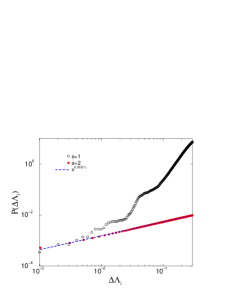
Figure 5: (Color online) Lifschitz tails on GSW graphs with $N=4\times 10^{4}$. Bullets: $s=1$, squares: $s=2$. Dashed line: power-law fitting: $\sim\Delta\Lambda_{i}^{0.55(1)}$.

VI Localization transition on scale-free networks

Up to know I showed agreement and success of the QMF-IPR method by predicting the RR effects in agreement with the expectations. Now I point out some limitations. Problems arise for example in case of SIS model on Barabasi-Albert (BA) networks Barabási and Albert (1999). These networks are generated by a linear preferential attachment rule, starting from a small fully connected seed ($N_{0}$). At each time step $s$, a new vertex (labeled by $s$) with $m$ edges is added to the network and connected to an existing vertex $s^{\prime}$ of degree $k_{s^{\prime}}$ with the probability $\Pi_{s\rightarrow s^{\prime}}=k_{s^{\prime}}/\sum_{s^{\prime\prime}=1}^{s^{\prime\prime}<s}k_{s^{\prime\prime}}$. By iterating the attachments for $N$ times one arrives to a graph with $N+N_{0}$ nodes with an asymptotic SF degree distribution $P(k)\simeq k^{-3}$.

A previous work basiscikk showed that for SIS models the IPR remained small in these networks, however uncertainties grew by increasing $N$. Now I compute IPR for a large number of disorder realizations for each each $N$ and show that $P(I)$ distributions become wide as $N\to\infty$, with the appearance on an additional peak, besides the one at zero. As shown on Fig. 6 the second peak becomes dominant for $N\geq 5\times 10^{5}$, suggesting a crossover to localization in the infinite size limit. In this analysis $m=3$ BA networks with $N_{0}=5$ were used.

Earlier dynamical simulations of the CP did not show deviations from the mean-field transition in case of $\gamma=3$ degree distribution, except for BA trees, especially when certain weighting schemes were applied BAGPcikk . Note, that for SIS model $\lambda_{c}=0$ is expected in the $N\to\infty$ limit, thus RR effects, if occur, could only slow down the relaxation towards the active state.

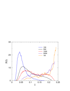
Figure 6: (Color online) Probability distribution of IPR of the $m=3$ BA SIS model for sizes $N=10^{4}$, $5\times 10^{4}$ $10^{5}$, $5\times 10^{5}$ and $N=10^{6}$ (from left to right).

To investigate this further I considered the SIS on uncorrelated configuration model (UCM) CBS05 , since one can control the degree distribution easily and these have been studied by various techniques. The UCMs were generated by the standard way. In a set of $N$ vertexes one assigns to each vertex $k_{i}$ number of “stubs”, drawn from the probability distribution $P(k)$, with the $k_{0}\leq k_{i}<k_{c}$ and the $\mod(\sum_{i}k_{i},2)=0$ constraints. The network is completed by connecting pairs of these stubs chosen randomly to form edges, respecting $k_{i}$ and avoiding self or multiple connections. A minimum degree $k_{0}=2$ and a structural cutoff $k_{c}=N^{1/2}$ was used to generate uncorrelated connected networks with probability one. The result of this construction is a random network, whose degrees are distributed according to $P(k)$ without degree correlations.

I generated the adjacency matrices for a large number of UCM graph realizations for degree distributions with $\gamma=4$, $3.5$, $3$, $2.8$, $2.5$ and performed the QMF analysis for sizes: $N=10^{3}$, $2\times 10^{3}$, $10^{4}$, $5\times 10^{4}$, $10^{5}$, $2\times 10^{5}$. The estimated threshold values $\lambda_{c}=1/y_{M}$ tend to zero in the $N\to\infty$ limit, in agreement with theoretical arguments for SIS: $\lambda_{c}\sim 1/N^{1/4}$ for $2.5<\gamma\leq 3$ and $\lambda_{c}\sim 1/N^{1/[2(\gamma-1)]}$ for $\gamma>3$ Fer14 ; CP10 . Power-law fits provided $\langle\lambda_{c}\rangle\sim 1/N^{0.25(1)}$ for $\gamma=2.5,3$ and $\langle\lambda_{c}\rangle\sim 1/N^{0.17(1)}$ for $\gamma=4$ (see Fig. 7).

The probability distributions of IPR values are also calculated and as the right inset of Fig. 7 shows they converge to a sharp peak at $I=0$ for $\gamma=2.5$, $2.8$, while they smear, similarly as in case of BA, suggesting a localization transition at $\gamma=3$ (see left inset of Fig. 7). For $\gamma=4$, $3.5$ the peaks of $P(I(N))$ are localized around $I\simeq 0.25$.

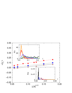
Figure 7: (Color online) Finite size scaling of QMF results of SIS on UCM networks. Mean value of $\lambda_{c}$ for $N=10^{3},...,2\times 10^{5}$ and for $\gamma=4$ (diamonds), $3$ (squares), $2.5$ (bullets). Lines correspond to power-law fits. Right inset: $P(I)$-s for $\gamma=2.5$ with network sizes increasing from right to left curves. Left inset: $P(I)$-s for $\gamma=3$ with network sizes increasing from the left to right curves.

The mean value results of the IPR distributions are summarized on Fig. 8. For $\gamma=2.5$ networks $\lim_{N\to\infty}\langle I(N)\rangle=0$, thus no sign of localization appears. On the other hand, for $\gamma=4$ the mean IPR remains finite and a localized network with $I(N)\to 0.26(1)$ can clearly be observed. Data are plotted on the $1/N^{0.3}$ scale, which shows the leading order finite size scaling in the best way. At $\gamma=3$ we can see a crossover towards eigenvector localization. The distribution of $\langle I(N)\rangle$ is very wide here as in case of the BA graph.

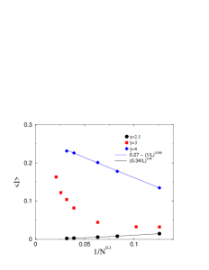
Figure 8: (Color online) Mean values of IPR on UCM graphs with $N=10^{3},...,2\times 10^{5}$. Rhombuses: $\gamma=4$ extrapolation $N\to\infty$ results in $I=0.26(1)$ (localization). Bullets: $\gamma=2.5$. For $\gamma=3$ (squares) a crossover (a localization transition) emerges.

The coefficients of the expansion $a_{1}$, $a_{2}$ and $a_{3}$ in Eq. (3) disappear as $\sim(1/N)$ in case of $\gamma\geq 3$. On the other hand for $\gamma<3$, $a_{1}$ decays slower than $\sim(1/N)$, while $a_{2}$ and $a_{3}$ are roughly zero, corresponding to a clear mean-field transition with $\beta=1$. Such change has been observed in wbacikk ; basiscikk in accordance with the emergence of RR effects.

I have also studied the Lifschitz tail above and below the localization transition in a similar way as before on UCM graphs with $N=10^{5}$ nodes. The spectrum gap grows by decreasing $\gamma$ as: $\Lambda_{2}=2.0166$ for $\gamma=4$, $\Lambda_{2}=2.0359$ for $\gamma=3$ and $\Lambda_{2}=2.0961$ for $\gamma=2.5$. This is in agreement with our expectations, because larger gap means more entangled networks, in which epidemic spreads quickly. The lowest $500$ eigenvalues are calculated and histogrammed using bin sizes $\delta\Lambda=0.0001$, following the drop of the $\Lambda_{1}=0$ eigenvalue. The $P(\Lambda_{i})$ distributions are shifted by $-\Lambda_{2}$ helping us to recognize possible power-laws on log.-log. plots. As Fig. 9 shows, in the localized phase ($\gamma=4$) a power-law distribution seems to emerge indeed, characterized by $P(\Delta\Lambda_{i})=2.258(12)(\Delta\Lambda_{i})^{1.52(1)}$. On the other hand in the delocalized phase, for $\gamma=2.5$, one can observe a faster than power-law behavior, which can be fitted well with the stretched a exponential form: $5000\exp(-3/(\Delta\Lambda)^{0.5})$, in agreement with the asymptotic of Eq. (15), valid for uncorrelated random networks. For comparison, a power-law fit assumption would lead to a large standard error of the regression coefficient: $\epsilon=0.142$.

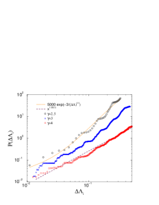
Figure 9: (Color online) Lifschitz tails of SIS on UCM graphs Bullets: $\gamma=4$, triangles: $\gamma=3$, squares: $\gamma=2.5$. Dashed line: power-law fitting with $\sim(\Delta\Lambda_{i})^{1.52(1)}$. Dotted line: least squares fitting with the stretched exponential form $5000\exp(-3/(\Delta\Lambda)^{0.5})$.

Finally, at the $\gamma=3$ localization transition point, the tail behavior at small $\Delta\Lambda$ deviates slightly away from a power-law, suggesting the lack of GP phase, in agreement with the numerical simulations of BAGPcikk done for the CP in BA networks. Assumption of a power-law fit form provides: $\epsilon=0.018$.

Unfortunately the differences observed between the power-law and stretched exponential tail behaviors are rather small. This is probably due to the limitation of computing high precision $P(\Lambda)$ for large sizes. This puts a question mark on the applicability of the Lifschitz tail method in general.

VII Conclusions

Probability distributions of the inverse participation ratio have been calculated in various network models exhibiting explicit or topological heterogeneities. Careful finite size scaling analysis pointed out the emergence of localization in generalized small world and scale-free models. This method describes well the GP singularities both in one-dimensional SIS with interaction disorder and in GSW-s with topological heterogeneity. Localization, appearing in the active phase signals GP singularities there. Former dynamical simulations in case of generalized small world networks Muñoz et al. (2010); GPCNlong ; MMNat support this. In infinite dimensional systems like ER graphs or BA networks GP-s with slow dynamics have been shown to appear only in weighted models Muñoz et al. (2010); GPCNlong ; BAGPcikk ; wbacikk ; Buo . In SF models with pure topological disorder the simulations have been concentrated on the location of the critical point by calculating stationary quantities FCP12 ; BCS13 ; Fer14 ; Ferrnew and visible GP effects have not been reported yet. Only loop-less BA trees showed non-trivial phase transition by very extensive density decay simulations BAGPcikk . This just corresponds to the localization point, thus one can expect more rare-region effects for $\gamma>3$ SF networks. Preliminary numerical simulations indicate a time window, with a power-law like approach to the steady state.

On the other hand the lower spectral tail of the Laplacian describes behavior in the inactive phase. In the linear approximation this is related to the dynamics of the order parameter. The predictive power of the Lifschitz tail method has been investigated and found qualitative agreement with the expectations. Finite systems exhibit spectral gaps, above which power-law tails were found, when GP behavior is expected. Fat tail distributions of the adjacency matrix of SF were already shown in DGMS03 . This study suggests the existence of SIS network models with fat-tailed Laplacians. However, calculation of the Lifschitz tail numerically is a demanding task, not much easier than simulation of the time dependent order parameter. Furthermore, since QMF predicts $\lambda_{c}=0$ for SF and GSW networks one cannot deeply be in the inactive phase of SIS, where the method is expected to work in the thermodynamic limit.

Application of these methods to SF networks results in a localization transition at $\gamma=3$ both for correlated and uncorrelated graphs. This is in agreement with the very recent simulation results, discussed in Ferrnew and with the threshold, where the degree fluctuations $\langle k^{2}\rangle$ diverge in the HMF approximation PV01 due to the strong heterogeneities. The localization in the active phase suggests dynamical RR effects for $\gamma>3$, like in the models presented in LSN12 . However, for SIS, where $\lambda_{c}=0$ is expected to be in the thermodynamic limit, this implies a smeared phase transition, with an algebraic decaying density in a time window towards the active steady state value. This scenario is feasible, because subspaces of an infinite dimensional graph can be RR-s with arbitrary topological dimensions exhibiting phase transition at different $\lambda$-s, as suggested in BAGPcikk . According to CPN12 for large $\gamma$-s hubs sustain the epidemic processes instead of the the innermost, dense core, thus one may expect that hubs play the role of RR-s here. In finite networks the smeared phase transition may also look like multiple phase transitions.

The success of the QMF method for describing GP behavior is demonstrated here for SIS in basic network models. However, the linearization Monthus ; KI11 ; JK13 and the complete neglection of dynamical fluctuations Fer14 warn for limitations on this relatively fast method, especially when the strong fluctuations override the localization effects. The appearance of strong RR effects above the upper critical dimension HoyosVojta supports, that QMF method is capable to predict exotic GP-s with off-critical, power-law singularities.

References

- (1) R. Albert and A.-L. Barabási, Rev. Mod. Phys. 74, (2002) 47.
- (2) S. N. Dorogovtsev and J. F. F. Mendes, Evolution of networks: From biological nets to the Internet and WWW, (Oxford Univ. Press Oxford, 2003).
- (3) M. E. J. Newman, Networks: An introduction, (Oxford Univ. Press Oxford, 2010).
- Harris (1974a) T. E. Harris, Ann. Prob. 2, 969 (1974a).
- Liggett (1985) T. M. Liggett, Interacting Particle Systems (Springer-Verlag, New York, 1985).
- (6) R. Pastor-Satorras and A. Vespignani, Evolution and Structure of the Internet: A Statistical Physics Approach (Cambridge University, Cambridge, 2004).
- (7) P. Moretti, M. A. Muñoz, Nature Communications 4, (2013) 2521.
- (8) N. T. J. Bailey, The Mathematical Theory of Infectious Diseases (Griffin, London, 1975), 2nd ed.; J. D. Murray, Mathematical Biology (Springer-Verlag, Berlin, 1993).
- (9) M. Boguña, C. Castellano and R. Pastor-Satorras, Phys. Rev. Lett. 111 (2013) 068701.
- Marro and Dickman (1999) J. Marro and R. Dickman, Nonequilibrium Phase Transitions in Lattice Models (Cambridge University Press, Cambridge, 1999).
- (11) G. Ódor, Rev. Mod. Phys. 76 (2004) 663
- Ódor (2008) G. Ódor, Universality in Nonequilibrium Lattice Systems (World Scientific, Singapore, 2008).
- (13) M. Henkel, H. Hinrichsen and S. Lübeck, Non-Equilibrium Phase Transitions vol. 1., Springer 2008
- Vojta (2006) T. Vojta, Journal of Physics A: Mathematical and General 39, R143 (2006).
- Muñoz et al. (2010) M. A. Muñoz, R. Juhász, C. Castellano, and G. Ódor, Phys. Rev. Lett. 105, 128701 (2010).
- Griffiths (1969) R. B. Griffiths, Phys. Rev. Lett. 23, 17 (1969).
- (17) S. Johnson, J. J. Torres, and J. Marro, PLoS ONE 8(1): e50276 (2013)
- (18) R. Pastor-Satorras and A. Vesignani, Phys. Rev. Lett. 86 (2001) 3200.
- (19) M. Karsai et al. Phys. Rev. E 83 (2011) 025102(R)
- (20) A. Haimovici, E. Tagliazucchi, P. Balenzuela and D. R. Chialvo, Phys. Rev. Lett. 110, 178101 (2013).
- (21) G. Ódor, Phys. Rev. E 89, 042102 (2014)
- (22) F. Iglói, C. Monthus, Phys. Rep. 412, 277-431, (2005)
- (23) B. Kramer and A. MacKinnon, Rep. Prog. Phys. 56, 1469 (1993).
- Boguñá et al. (2009) M. Boguñá, C. Castellano, and R. Pastor-Satorras, Phys. Rev. E 79, 036110 (2009).
- (25) S. C. Ferreira, C. Castellano, R. Pastor-Satorras, Phys. Rev. E 86, 041125 (2012)
- (26) Angélica S. Mata, Ronan S. Ferreira, Silvio C. Ferreira, New J. Phys. 16 (2014) 053006
- (27) D. Chakrabarti, Y. Wang, C. Wang, J. Leskovec, and C. Faloutsos, ACM Trans. Inf. Syst. Secur. 10, 1 (2008).
- (28) P. Van Mieghem, J. Omic, and R. Kooij, IEEE ACM T. Network. 17, 1 (2009).
- (29) C. Castellano and R. Pastor-Satorras, Phys. Rev. Lett. 105 (2010) 218701.
- (30) A. V. Goltsev, S. N. Dorogovtsev, J. G. Oliveira, and J. F. F. Mendes, Phys. Rev. Lett. 109, 128702 (2012)
- (31) G.Ódor, Phys. Rev. E 87, (2013) 042132.
- (32) G.Ódor, Phys. Rev. E 88, (2013) 032109.
- (33) C. Monthus, T. Garel, J. Phys. A: Math. Theor. 44 (2011) 085001.
- (34) I. A. Kovács and F. Iglói, J. Phys.: Condens. Matter 23, 404204 (2011).
- (35) R. Juhász and I. A. Kovács, J. Stat. Mech. (2013) P06003.
- (36) P. Villegas, P. Moretti, M. A. Muñoz, Sci. Rep. 4, (2014), 5990
- (37) A. Nüsser, J. Phys. A, 24 (1991) 2355.
- (38) O. Khorunzhiy, W. Kirsch, and P. Ml̈ler, Ann. Appl. Probab. 16 (2006), 295-309.
- (39) F. R. K. Chung (1997). Spectral Graph Theory, Amer. Math. Soc., Providence, RI.
- (40) P. V. Mieghem, Graph Spectra for Complex Networks, (Cambridge University Press, Cambridge 2011).
- (41) A. N. Samukhin, S. N. Dorogovtsev and J. F. F. Mendes, PRB 77, 036115 (2008).
- (42) S. N. Taraskin et al, Phys. Rev. E. 7, 016111 (2005).
- (43) M. Barahona and L. M. Pecora, Phys. Rev. Lett 89 (2002) 054101
- (44) L. Donetti, F. Neri and M. Muñoz, J. of Stat. Mech (2006) P08007.
- (45) P. Van Mieghem, Eur. Phys. Lett. 97, 48004 (2012).
- (46) P. Van Mieghem and J. Omic, Delft University of Technology, report2008081, arxiv.org:1306.2588.
- (47) P. Van Mieghem, Computing 93, (2011) 147-169.
- (48) A. J. Noest, Phys. Rev. Lett. 57, 90 (1986); A. J. Noest, Phys. Rev. B 38, 2715 (1988).
- (49) H. K. Janssen, Phys. Rev. E 55, 6253 (1997).
- (50) A. G. Moreira and R. Dickman, Phys. Rev. E 54, R3090 (1996).
- (51) M. M. de Oliveira and S. C. Ferreira, JSTAT P11001 (2008)
- (52) T. Vojta, A. Farquhar, and J. Mast, Phys. Rev. E 79, 011111 (2009).
- (53) J. Hooyberghs, F. Iglói and C. Vanderzande, Phys. Rev. Lett., 90, 100601 (2003)
- (54) http://www.gnu.org/software/octave
- (55) M. Aizenman and C.M. Newman, Commun. Math. Phys. 107, 611 (1986).
- (56) J.M. Kleinberg, Nature 406, 845 (2000).
- (57) I. Benjamini and N. Berger, Rand. Struct. Alg. 19, 102 (2001).
- Barabási and Albert (1999) A.-L. Barabási and R. Albert, Science 286, 509 (1999).
- (59) R. Juhász, Phys. Rev. E 78, 066106 (2008).
- (60) R. Juhász, G. Ódor, Phys. Rev. E 80, 041123 (2009)
- (61) R. Juhász, G. Ódor, C. Castellano and M. Muñoz, Phys. Rev. E 85, 066125 (2012)
- (62) G.Ódor and R. Pastor-Satorras, Phys. Rev. E 86, (2012) 026117.
- (63) T. Vojta, J. A. Hoyos, Phys. Rev. Lett. 112, 075702 (2014); T. Vojta, J. Igo, J. A. Hoyos, arXiv:1405.4337
- (64) R. Juhász, J. Stat. Mech. (2013) P10023
- (65) P. Erdős and A. Rényi, A. (1959) Publ. Math. 6, 290–291.
- (66) M. Catanzaro, M. Boguña and R. Pastor-Satorras, Phys. Rev. E 71 (2005) 027103.
- (67) S. N. Dorogovtsev, A. V. Goltsev, J. F. F. Mendes, Phys. Rev. E 68, 046109.
- (68) A. S. Mata, S. C. Ferreira, arXiv:1403.6670
- (69) H. K. Lee, P.-S. Shim and J. D. Noh, Phys. Rev. E 87, 062812 (2013)
- (70) C. Castellano and R. Pastor-Satorras, Sci. Rep. 2 (2012) 371.
- (71) C. Buono, F. Vazquez, P. A. Macri, L. A. Braunstein, Phys. Rev. E 88, 022813 (2013)