From quantum-mechanical to classical dynamics in the central-spin model

Abstract

We discuss the semiclassical and classical character of the dynamics of a single spin $1/2$ coupled to a bath of non-interacting spins $1/2$. On the semiclassical level, we extend our previous approach presented in D. Stanek, C. Raas, and G. S. Uhrig, Phys. Rev. B 88, 155305 (2013) by the explicit consideration of the conservation of the total spin. On the classical level, we compare the results of the classical equations of motions in absence and presence of an external field to the full quantum result obtained by density-matrix renormalization (DMRG). We show that for large bath sizes and not too low magnetic field the classical dynamics, averaged over Gaussian distributed initial spin vectors, agrees quantitatively with the quantum-mechanical one. This observation paves the way for an efficient approach for certain parameter regimes.

I Introduction & Motivation

Single electron or hole spins confined in a quantum dot are promising candidates for the realization of quantum bits (qubits).Loss and DiVincenzo (1998); Hanson et al. (2007); Urbaszek et al. (2013) The requirements for a system to be a good candidate for a quantum computer are summarized in the well-known criteria of DiVincenzo.DiVincenzo (2000) One essential ingredient is the existence of long decoherence times to dispose of long storage times for the quantum information or to make a large number of gate operations possible. Hence, a detailed understanding of the real-time evolution of the qubit induced by the interaction with its environment is crucial.

In bulk solids, the dominating contribution to the decoherence of an electronic spin, taken as qubit, is usually based on spin-orbit coupling. However, it has been shown that the relaxation Khaetskii and Nazarov (2000, 2001) and the dephasingGolovach et al. (2004) due to spin-orbit coupling of an electron spin confined in a quantum dot is strongly suppressed. Instead, the hyperfine coupling between the electron spin and the surrounding nuclear spins in the dot is the major player.Merkulov et al. (2002); Schliemann et al. (2003) This situation is well captured by the central-spin or Gaudin model (CSM)Gaudin (1976, 1983)

$$H =-h_{0}S^{z}_{0}+\vec{S}_{0}\cdot\sum\limits_{i=1}^{N}J_{i}\vec{S}_{i},$$ (1)

where a central spin $\vec{S}_{0}$ in an external field $h_{0}$ interacts with $N$ non-interacting bath spins $\vec{S}_{i}$. The coupling constants $J_{i}$ are distributed randomly because their values are proportional to the probability $|\psi(\vec{r}_{i})|^{2}$ [$\psi(\vec{r})$ being the wave vector of the confined electron] that the electron is present at the site of the nucleus $i$ located randomly in the dot.Merkulov et al. (2002); Schliemann et al. (2003) It is convenient to represent the bath by the operator

$$\vec{A} :=\sum\limits_{i=1}^{N}J_{i}\vec{S}_{i},$$ (2a)

which acts on all bath spins weighted with their corresponding coupling constant. It can be interpreted as an effective three-dimensional magnetic field created by the bath spins called the Overhauser field. The Hamiltonian (1) simplifies to

$$H =-h_{0}^{\phantom{z}}S^{z}_{0}+\vec{S}_{0}\cdot\vec{A}.$$ (2b)

We take the external field $h_{0}$ to be restricted to the central spin $\vec{S}_{0}$ because the Zeeman splitting of the nuclear spins is much smaller due to the small magnetic moments of the nuclei. The magnetic moment of the electron is about three orders of magnitude larger. The dipolar interaction between nuclear bath spins is not considered because it affects the physics of the model only on a much larger time scale than the hyperfine interaction.Merkulov et al. (2002) The intrinsic energy scale of a typical self-assembled quantum dot is of the order of $10^{-5}\,\mathrm{eV}$.Merkulov et al. (2002); Schliemann et al. (2003); Lee et al. (2005); Petrov et al. (2008) Experiments are usually performed at temperatures in the range $T=6$–$50\,\mathrm{K}$ corresponding to thermal energies $k_{\mathrm{B}}T\approx 10^{-4}$–$10^{-3}\,\mathrm{eV}$.Hernandez et al. (2008); Greilich et al. (2009) Thus, the energy scale of the thermal fluctuations is at least one order of magnitude larger than the intrinsic energy scale of the spins in the quantum dot. This implies that the temperatures occurring in experiment can be taken to be infinite so that the nuclear spins are initially completely unpolarized.

The real-time evolution of the central spin can be computed by numerical techniques such as exact diagonalizationSchliemann et al. (2003); Cywiński et al. (2010) or the Chebyshev expansion.Dobrovitski and De Raedt (2003); Hackmann and Anders (2014) Analytical solutions can be derived by means of the Bethe ansatz for strongly polarized initial states.Bortz and Stolze (2007a, b) Recently, a combination of the algebraic Bethe ansatz and Monte Carlo sampling was able to access unpolarized initial mixtures with up to 48 bath spins.Faribault and Schuricht (2013a, b) Much larger systems can be treated by DMRG, but generically the reliability of the results is limited in time due to the growing truncation error occurring in the DMRG sweeps.Stanek et al. (2013) We will see an exception to this rule for strong magnetic fields where this restriction turns out to be much less severe. Approaches based on a non-Markovian master equation give access to larger bath sizes, but they are limited to sufficiently strong external fields.Coish and Loss (2004); Breuer et al. (2004); Fischer and Breuer (2007); Ferraro et al. (2008); Barnes et al. (2012) With cluster expansion techniques, the closely related problem of the dephasing of the central spin due to spectral diffusion can be treated.Witzel et al. (2005); Witzel and Das Sarma (2006); Maze et al. (2008); Yang and Liu (2008, 2009); Witzel et al. (2012)

Moreover, the dynamics of the central spin was frequently studied on the level of semiclassical or classical models. These methods comprise a variety of approaches, for instance, the replacement of the bath by an effective time-dependent field.Erlingsson and Nazarov (2002, 2004); Merkulov et al. (2002); Stanek et al. (2013) As a first approximation, the bath may be regarded as frozen, i.e, the Overhauser field is constant. Subsequently, random fluctuations of the bath due to the interaction with the central spin can be included.Merkulov et al. (2002) Assuming that the Overhauser field can be described as stochastic field, the fluctuations of the central spin can be found from solution of the Bloch equation of the Langevin type.Glazov and Ivchenko (2012); Hackmann et al. (2014)

Furthermore, it was argued that the classical trajectories of the CSM resulting from the saddle point approximation of the spin-coherent path integral representation describe the central-spin dynamics well because the quantum fluctuations become less important for large numbers of bath spins.Chen et al. (2007) Similarly, a large number of bath spins was accessed by combining the so-called $P$ representation of the density matrix with time-dependent mean-field theory.Al-Hassanieh et al. (2006); Zhang et al. (2006)

The goal of the present paper is to study to what extent the quantum-mechanical dynamics of the central spin can be described by simpler models. We will focus on the semiclassical and the classical model. By comparison of fully quantum-mechanical results with the results from these two models we establish for which regimes the simpler calculations can be regarded as essentially equivalent to the quantum-mechanical ones. Thereby, certain future investigations can be done much more efficiently because the evaluation of the simpler models is sufficient. To our knowledge, a detailed comparison between the classical and quantum behavior in the CSM has not been conducted so far.

For our proof-of-principle study, we restrict ourselves to spins $S=1/2$ and discuss a generic uniform distribution $J_{i}\in[0,J_{\mathrm{c}}]$ where the cutoff $J_{\mathrm{c}}$ is determined by the total energy scale $J_{\mathrm{q}}$ of the CSM. Since we deal with an unpolarized bath, the energy scale is given by the root of the second moment of the couplings Merkulov et al. (2002)

$$J_{\mathrm{q}}^{2} :=\sum\limits_{i=1}^{N}J_{i}^{2}.$$ (3)

Consequently, the natural unit of time for the fast dynamics is given by $1/J_{\mathrm{q}}$ which we use in the sequel (we set $\hbar$ to unity). We pick equidistant couplings from the interval $[0,J_{\mathrm{c}}]$

$$J_{i} =\sqrt{\frac{6N}{2N^{2}+3N+1}}\frac{N+1-i}{N}J_{\mathrm{q}},$$ (4)

where $i\in\{1,\ldots,N\}$ to represent a uniform distribution of the $J_{i}$ in $[0,J_{\mathrm{c}}]$.

The paper is organized as follows: In Sect. II, we discuss the semiclassical approach. The described ansatz incorporates the conservation of the total spin leading to a good description up to intermediate time scales. The classical equations of motion are discussed in Sect. III with and without an external magnetic field. A detailed comparison with the DMRG results for the quantum model is presented to verify the validity of the classical picture. Finally, our findings are concluded in Sect. IV.

II Semiclassical model

The classical character of the bath is to be expected for a large number of bath spins. This has been made rigorous by an analytic argument for the operator norm and the commutator of the Overhauser field.Stanek et al. (2013) Further support stems from the comparison to DMRG results for zero external field. Hence one may replace the operator $\vec{A}$ of the Overhauser field by a classical field $\vec{\eta}(t)$ to obtain the semiclassical Hamiltonian

$$H_{\mathrm{sc}} =\vec{\eta}\left(t\right)\cdot\vec{S}_{0}.$$ (5)

The central spin $\vec{S}_{0}$ is still treated on the quantum level. In addition, the dynamics of the classical field $\vec{\eta}$ is assumed to be stochastic and of Gaussian statistics according to the central limit theorem. We stress that this assumption neglects any backaction effects of the central spin on the fluctuations of the Overhauser field. The fluctuations are fully defined by the autocorrelation functions

$$g_{\alpha\beta}\left(t_{1}-t_{2}\right) =\overline{\eta_{\alpha}\left(t_{1}\right)\eta_{\beta}\left(t_{2}\right)}$$ (6a)

with $$\alpha,\beta\in\{x,y,z\}$$ and their mean values

$$\overline{\eta_{\alpha}\left(t\right)} =0.$$ (6b)

Without loss of generality, the mean values are taken to vanish because a finite value can be interpreted as a contribution of an external magnetic field. In passing from the quantum to the semiclassical model, the autocorrelation functions $g_{\alpha\beta}(t)$ are identified with the autocorrelations $\braket{A^{\alpha}(t)A^{\beta}(0)}$ of the Overhauser field, see Ref. Stanek et al., 2013 for details.

In previous works, the comparison between the semiclassical model and the quantum model has revealed a very good agreement on short time scales up to $t\approx 10\,J_{\mathrm{q}}^{-1}$ or for finite frequencies.Stanek et al. (2013); Hackmann et al. (2014) However, for longer times, the autocorrelation function of the central spin always displays a pronounced decay in the semiclassical calculation which does not coincide with what is found in quantum-mechanical calculations, for an example see the red dashed curves labeled “Langevin 1” in Fig. 2. The neglect of conservation laws of the full quantum model due to the semiclassical treatment is one reason for this behavior as we will illustrate below.

For details of the calculation “Langevin 1”, we refer the reader to Ref. Stanek et al., 2013 and to Sect. II.3 below. One key element is that the autocorrelations of the Overhauser field are taken from the numerical DMRG calculation.

II.1 Conservation of the total spin

An obvious conserved quantity in the central spin model is the total spin

$$\vec{I} =\sum\limits^{N}_{i=0}\vec{S}_{i}.$$ (7)

By construction, the numerical DMRG captures the conservation of the total spin and all other conservation laws in the CSM to the degree of its numerical accuracy. However, this does not hold for the semiclassical model defined in Eq. (5) which obviously does not display a conservation law for the fluctuating Overhauser field $\vec{\eta}$.

To improve the reliability of the semiclassical results as predictions for the quantum-mechanical calculation, we show here how the conservation of the total spin $\vec{I}$ can be incorporated in the semiclassical model and discuss its effect. To this end, we study the slightly modified Hamiltonian

$$H^{\prime} =\vec{S}_{0}\cdot\sum\limits_{i=0}^{N}J_{i}\vec{S}_{i}$$ (8)

for the quantum CSM. The central spin $\vec{S}_{0}$ has been included in the sum which was restricted originally to the bath spins. For $S=1/2$, the additional contribution induces only a constant shift $3J_{0}/4$ in the Hamiltonian. Thus, it has no influence on the dynamics of the model. The arbitrary coupling constant of the central spin is assigned the mean value of all couplings

$$J_{0} :=\frac{1}{N}\sum\limits^{N}_{i=1}J_{i}.$$ (9)

Consequently, the fluctuating field

$$\vec{A} =\sum\limits_{i=0}^{N}J_{i}\vec{S}_{i}$$ (10a)

comprises the central spin $$\vec{S}_{0} \vec{A}$$ in addition to the bath spins. To take the conservation of the total spin into account, we rewrite in the form

$$\vec{A} =\vec{A}_{0}+\Delta\vec{A}.$$ (10b)

The part

$$\vec{A}_{0} =J_{0}\vec{I}$$ (11a)

is conserved and thus constant in time while the contribution

$$\Delta\vec{A} =\sum\limits_{i=1}^{N}\left(J_{i}-J_{0}\right)\vec{S}_{i}$$ (11b)

comprises the fluctuating part.

The temporal constancy $\vec{A}_{0}(t)=\vec{A}_{0}(0)$ implies that the correlation of the conserved part is given by the constant expression

$$\braket{A^{\alpha}_{0}\left(t\right)A^{\beta}_{0}\left(0\right)} =J_{0}^{2}\frac{N+1}{4}\delta_{\alpha\beta}.$$ (12a)

Here we focus on the zero-field limit where all nondiagonal correlations vanish and the diagonal correlations are isotropic: $$g(t):=g_{\alpha\alpha}(t)$$. However, we continue to use the general notation so that the present discussion can easily be extended to other symmetries.

It is important to realize that the conserved and the fluctuating parts are independent at all times in the sense that their correlations vanish

$$\braket{A^{\alpha}_{0}\left(t\right)\Delta A^{\beta}_{0}\left(0\right)} =\braket{A^{\alpha}_{0}\left(0\right)\Delta A^{\beta}_{0}\left(0\right)}$$ (12b)

$$=\frac{J_{0}}{4}\delta_{\alpha\beta}\sum\limits_{i=0}^{N}\left(J_{i}-J_{0}\right)$$ (12c)

$$=0.$$ (12d)

Thus, the autocorrelation function of the Overhauser field $\vec{A}$ acquires the form

$$g_{\alpha\beta}\left(t\right) =J_{0}^{2}\frac{N+1}{4}\delta_{\alpha\beta}+\Delta g_{\alpha\beta}\left(t\right)$$ (13a)

with

$$\Delta g_{\alpha\beta}\left(t\right) :=\braket{\Delta A^{\alpha}\left(t\right)\Delta A^{\beta}\left(0\right)}.$$ (13b)

Next, we address the central spin $\vec{S}_{0}$ which is treated similarly to the field $\vec{A}$ by splitting it into a constant and a fluctuating part

$$\vec{S}_{0} =\frac{1}{N+1}\vec{I}+\Delta\vec{S}_{0},$$ (14a)

where the fluctuating part reads

$$\Delta\vec{S}_{0} =\frac{N}{N+1}\vec{S}_{0}-\frac{1}{N+1}\sum\limits_{i=1}^{N}\vec{S}_{i}$$ (14b)

and the fraction $\vec{I}/(N+1)$ of the total spin $\vec{I}$ (7) is the conserved, constant contribution. Like for $\vec{A}$, there is no correlation between the constant and the fluctuating parts for any time

$$\braket{I^{\alpha}\left(t\right)\Delta S_{0}^{\beta}\left(0\right)} =\braket{I^{\alpha}\left(0\right)\Delta S_{0}^{\beta}\left(0\right)}$$ (15a)

$$=\frac{1}{4}\frac{N}{N+1}-N\frac{1}{4}\frac{1}{N+1}$$ (15b)

$$=0.$$ (15c)

Consequently, the autocorrelation function of the central spin $\vec{S}_{0}$ is given by

$$\braket{S^{\alpha}_{0}\left(t\right)S^{\beta}_{0}\left(0\right)} =\delta_{\alpha\beta}\frac{1}{4}\frac{1}{N+1}+\Delta c_{\alpha\beta}\left(t\right)$$ (16a)

with

$$\Delta c_{\alpha\beta}\left(t\right) :=\braket{\Delta S^{\alpha}_{0}\left(t\right)\Delta S^{\beta}_{0}\left(0\right)}.$$ (16b)

Note that the conserved fraction [first term on the right hand side of Eq. (16a)] vanishes for infinitely large systems $N\to\infty$.

In the above way, the conserved part is separated from the fluctuating part for both the central spin and the Overhauser field $\vec{A}$. We incorporate this concept into the semiclassical model by considering the Hamiltonian

$$H_{\mathrm{sc}}^{\prime} =\vec{\eta}\left(t\right)\cdot\Delta\vec{S}_{0}$$ (17)

which refers to the fluctuating part of the central spin only. Since the conserved part is constant, it does not enter in $H_{\mathrm{sc}}^{\prime}$. As before, the fluctuating field $\vec{\eta}(t)$ is a random Gaussian variable. Its correlation function is defined by $g_{\alpha\beta}(t)$ in Eq. (13a) involving the separate treatment of the fluctuating and the conserved parts of $\vec{A}$ in Eq. (10b). Thus, the conservation of the fraction of the Overhauser field, which is proportional to the total spin, is built in.

Inserting the expression for $\Delta\vec{S}_{0}$ from Eq. (17), the semiclassical Hamiltonian becomes

$$H_{\mathrm{sc}}^{\prime} =\sum\limits_{i=0}^{N}h_{i}$$ (18a)

where

$$h_{0} :=\frac{N}{N+1}\vec{\eta}\left(t\right)\cdot\vec{S}_{0}$$ (18b)

$$h_{i} :=-\frac{1}{N+1}\vec{\eta}\left(t\right)\cdot\vec{S}_{i},\ \ \ i\in\left\{1,2,\ldots,N\right\}.$$ (18c)

On this level of description, the time evolution of the bath spins $\vec{S}_{i},i>0$ is completely independent from one another. The fluctuating part $\Delta c_{\alpha\beta}\left(t\right)$ of the autocorrelation function of the central spin can be calculated by

$$\Delta c_{\alpha\beta}\left(t\right) =\left(\frac{N}{N+1}\right)^{2}\Delta c_{\alpha\beta}^{(0)}\left(t\right)+\frac{N}{\left(N+1\right)^{2}}\Delta c_{\alpha\beta}^{(i)}\left(t\right)$$ (19a)

with the two independent contributions

$$\Delta c_{\alpha\beta}^{(0)}\left(t\right) :=\braket{S^{\alpha}_{0}\left(t\right)S^{\beta}_{0}\left(0\right)}$$ (19b)

$$\Delta c_{\alpha\beta}^{(i)}\left(t\right) :=\braket{S^{\alpha}_{i}\left(t\right)S^{\beta}_{i}\left(0\right)}$$ (19c)

where the former [Eq. (19b)] acquires its dynamics from the Hamiltonian $h_{0}$ in Eq. (18b) and the latter [Eq. (19c)] acquires its dynamics from the Hamiltonian $h_{i}$ in Eq. (18c).

In total, two independent runs of the code are required for simulating this enhanced semiclassical model which respects the conservation of the total spin. The run for the Hamiltonian $h_{0}$ involves the strong coupling $\propto N/(N+1)$ between central spin and bath. Thus, the contribution $\Delta c_{\alpha\beta}^{(0)}\left(t\right)$ dominates the fast dynamics of the autocorrelation function $\braket{S^{\alpha}_{0}\left(t\right)S^{\beta}_{0}\left(0\right)}$. In contrast, the coupling $-1/(N+1)$ between a single bath spin $\vec{S}_{i}$ and $\vec{\eta}(t)$ is small, in particular for large baths. Consequently, the Hamiltonian $h_{i}$ induces only a very slow dynamics. In addition, the weight factors in Eq. (19a) imply that the fast dynamics $\propto N/(N+1)$ is dominating anyway due to an extra factor $N$. Note, that for infinitely large systems with $N\to\infty$ the fast dynamics is the only one remaining. The calculations on this level of the semiclassical model are labeled “Langevin 2” in Fig. 2. More details of the calculations are given below in Sect. II.3.

II.2 The central spin as classical vector

In the above introduced modification “Langevin 2” of the random noise simulation, the central spin is treated on the quantum level, while the bath is a classical variable. However, the precession of a quantum spin in an external field is identical to the one of a classical vector in $\mathds{R}^{3}$ due to the linearity of the equations of motion. It implies that the quantum-mechanical expectation values follow exactly the classical equations of motion according to Ehrenfest’s theorem. Thus, we go one step further and replace the quantum-mechanical central spin by a classical vector in the simulations of the semiclassical model. Otherwise, we keep the separation in a conserved constant part and a fluctuating decaying part.

We recall the semiclassical Hamiltonian (17) and insert the expression for the fluctuating part $\Delta\vec{S}_{0}$ of the central spin defined in Eq. (14a)

$$H_{\mathrm{sc}} =\vec{\eta}\left(t\right)\left(\vec{S}_{0}-\frac{1}{N+1}\vec{I}\right).$$ (20)

According to Eq. (10b), the Gaussian fluctuation $\vec{\eta}(t)$ can be written as

$$\vec{\eta}\left(t\right) =J_{0}\vec{I}+\Delta\vec{\eta}\left(t\right).$$ (21)

Since the Hamiltonian (20) is a classical Hamiltonian, one easily deduces the two corresponding equations of motion:

$$\frac{\mathrm{d}}{\mathrm{d}t}\vec{S}_{0} =\vec{\eta}\left(t\right)\times\vec{S}_{0}$$ (22a)

$$\frac{\mathrm{d}}{\mathrm{d}t}\vec{I}_{\phantom{0}} =-\frac{1}{N+1}\vec{\eta}\left(t\right)\times\vec{I},$$ (22b)

where all spins are classical vectors in $\mathds{R}^{3}$. We also adopt the former expression for the autocorrelation function:

$$\overline{S^{\alpha}_{0}\left(t\right)S^{\beta}_{0}\left(0\right)} =\frac{1}{4}\frac{1}{N+1}\delta_{\alpha\beta}+\Delta c_{\alpha\beta}\left(t\right)$$ (23a)

with

$$\Delta c_{\alpha\beta}\left(t\right) :=\overline{\left(S^{\alpha}_{0}-\frac{1}{N+1}I^{\alpha}\right)\Big{(}t\Big{)}\left(S^{\beta}_{0}-\frac{1}{N+1}I^{\beta}\right)\Big{(}0\Big{)}}.$$ (23b)

To distinguish the latter expressions from the quantum description, the expectation values are denoted by an overbar and not by Dirac brackets $\left<.\right>$.

The equations of motion (22) can easily be integrated using standard methods and subroutines, for instance Runge-Kutta integration. As in the previous section for the improved semiclassical calculation, two independent runs of the integration are required: one for the precession due to (22a) for a strong coupling and another for the precession due to (22b) for a weak coupling to the random field $\vec{\eta}(t)$, Eq. (21). Except for this change, the integration can be carried out with the same code.

In the simulation, we sample the Gaussian fluctuations $\Delta\vec{\eta}(t)$ complying with the autocorrelation function $\Delta g_{\alpha\beta}(t)$ defined in Eq. (13b). However, which initial values are to be taken for $I^{\alpha}$ and $\Delta S_{0}^{\alpha}(0)$? We only have information on the averages: the mean values, corresponding to expectation values, vanish. However, the equal-time correlations are finite and known from the quantum-mechanical counterparts. Thus, we choose random initial values drawn from Gaussian distributions, which reproduce for $t=0$ the quantum-mechanical correlations. Concretely, we know the variance for a single component of the total spin to be

$$\braket{\left(I^{\alpha}\left(0\right)\right)^{2}} =\frac{N+1}{4}.$$ (24a)

For a single component of the fluctuating part $$\Delta S_{0}^{\alpha}(t) t=0$$, the initial variance at is given by the expression

$$\braket{\left(\Delta S^{\alpha}_{0}\left(t\right)\right)^{2}} =\frac{1}{4}\frac{N}{N+1}.$$ (24b)

The initial values enter in the equations of motion (22) as well as in the autocorrelation function $$\overline{S^{z}_{0}(t)S^{z}(0)}$$ of the central spin.

Sampling the Gaussian fluctuations $\Delta\vec{\eta}(t)$ and the initial values sufficiently well we determine the correlations by averaging over a large number $M$ of runs at each instant $t$. The resulting data are shown in Fig. 2 labeled by “Langevin 3”.

II.3 Semiclassical results for zero field

Here, we present results for the three approaches labeled “Langevin 1”, “Langevin 2”, and “Langevin 3” and compare them to the full quantum-mechanical DMRG results. The impact of the conservation of the total spin on the semiclassical calculation is a particular focus.

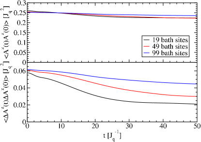
Figure 1: (Color online) (Top) Autocorrelation $\braket{A^{z}(t)A^{z}(0)}$ as defined in Eq. (10b). (Bottom) Separated fluctuating part $\braket{\Delta A^{z}(t)\Delta A^{z}(0)}$. Both are obtained by DMRG; the total discarded weight does not exceed $10\,\%$ at $t\approx 50/J_{\mathrm{q}}$, for further discussion see main text.

Before we consider the dynamics of the central spin we have to address the autocorrelation of the Overhauser field $\vec{A}$ defined in Eq. (10b). This is mandatory because we need the correlations of the noise as input for any semiclassical calculation. In the calculations presented below, we will use the exact autocorrelation of the Overhauser field for this purpose. Of course, one may object that no semiclassical calculation is needed if we perform a DMRG calculation anyway. While this is true, we will see that one understands the essentials of the central-spin dynamics better from the semiclassical calculations.

In the upper panel of Fig. 1, the DMRG results for the total autocorrelation of the Overhauser field including the constant part are depicted. In the lower panel, the fluctuating part $\Delta\vec{A}$ is plotted. The data are obtained from the DMRG implementation for the CSM involving a purified initial state describing the disordered bath and the time evolution based on the Trotter-Suzuki decomposition.Friedrich (2006); Stanek et al. (2013) Beyond the time range shown the total discarded weight starts exceeding 10%. The total (accumulated) discarded weight comprises the sum of the discarded weight in the reduced density matrix of all involved DMRG basis truncations up to the given time including the DMRG buildup and the DMRG sweeps. The percentage of total discarded weight implies that the deviations of generic expectation values can be in the same order of about 10%. But the increase is roughly exponential as observed earlier, cf. Ref. Stanek et al., 2013. This means that the relative error at $t\approx 45/J_{\mathrm{q}}$ is $1\%$ and at $t\approx 40/J_{\mathrm{q}}$ it is $0.1\%$ and so on. Thus the results are very reliable except close to the maximum times shown.

The lower panel demonstrates that the fluctuating part is indeed small compared to the constant one. Moreover, it is decreasing so that for large times one can expect that it vanishes completely and only the sizable constant part remains. Compared to the results in Ref. Stanek et al., 2013 the definition of the Overhauser field is changed because it includes the central spin itself now. This inclusion induces slightly longer lasting correlations between the fluctuations that should stabilize the autocorrelation of the central spin as well. As before in Ref. Stanek et al., 2013, the autocorrelation converges towards $\braket{A^{z}(t)A^{z}(0)}=J_{\mathrm{q}}^{2}/4$ for $N\rightarrow\infty$.

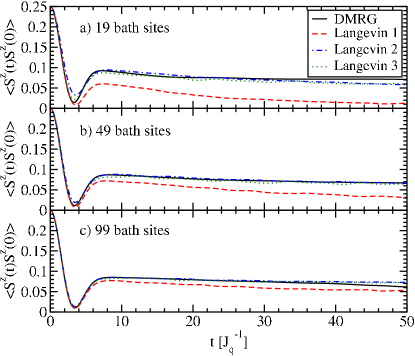
Figure 2: (Color online) Autocorrelation of the central spin up to intermediate time scales. In each panel, the results of the semiclassical calculations are compared to the corresponding DMRG result. All curves involving random noise have been obtained for $M=50\,000$ fluctuations, i.e., $M$ different time series $\vec{\eta}(t)$ and initial vectors are generated and the resulting central-spin evolutions are averaged.

For the simulation of the random noise, a large number $M$ of time series $\vec{\eta}(t)$ and initial vectors are sampled. Technically, correlated noise obeying a known autocorrelation $g(t)$ or $\Delta g(t)$ is generated from Gaussian distributed random variables by means of the eigen decomposition of the covariance matrix. The latter is obtained from the autocorrelations $\braket{A^{z}(t)A^{z}(0)}$ or $\braket{\Delta A^{z}(t)\Delta A^{z}(0)}$ discretized in time and taken from a DMRG calculation. The classical or quantum-mechanical time integrations are carried out easily for each time series $\vec{\eta}(t)$ because we are only dealing with a two-level system or a classical three-component vector. Finally, the average over the resulting $M$ time evolutions is computed. The concomitant statistical relative errors are estimated by $1/\sqrt{M}$.

The results for the autocorrelation $\braket{S^{z}_{0}(t)S^{z}_{0}(0)}$ of the central spin are presented in Fig. 2. For each bath size, we compare the DMRG result with the results obtained from the three semiclassical approaches introduced in the previous sections. If the conservation of the total spin is explicitly included, the central spin is treated on the operator level (Langevin 2) and as a classical vector (Langevin 3). As expected, however, this does not make any noticeable, statistically relevant difference for larger baths.

In contrast, the difference between Langevin 1 (without conservation of spin) and Langevin 2 or 3 (with conservation of spin) is significant. The data clearly show the importance of treating conserved quantities properly. The explicit conservation of the total spin leads to a substantial improvement of the results, which decay slower than in Langevin 1 in agreement with DMRG. The agreement with DMRG improves quickly with increasing system size. Up to the times displayed, the agreement of Langevin 2 or 3 with the DMRG data is excellent for the larger bath. We attribute the fact that for 99 bath sites the DMRG data fall below the semiclassical result beyond about $t\approx 40J_{\mathrm{q}}^{-1}$ to the growing inaccuracy of the DMRG data for growing $t$.

In view of the above finding, the question arises whether the semiclassical result stays close to the true quantum-mechanical result for all times. The answer is “no”. If the semiclassical computation is extended to long times $t\gg 50J_{\mathrm{q}}^{-1}$ assuming even that the Overhauser field autocorrelation does not decrease further beyond $t=50J_{\mathrm{q}}^{-1}$ one finds a decrease of the autocorrelation of the central spin down to a small value which is protected by the conservation of the total spin. However, this fraction is small; it scales like $1/N$ for $N\to\infty$, i.e., it is zero for infinite systems.

This is in contrast to the rigorously established behavior that a finite spin-spin correlation persists for all times if the average coupling is finite.Uhrig et al. (2014) This observation stems from Mazur’s inequality. It turns out that the conservation of the total spin is only one ingredient, but the conservation of the total energy is another important prerequisite. Only the energy conservation leads to a lower bound to the spin-spin correlation of the central spin which does not vanish for $N\to\infty$ if the average coupling remains finite. Thus we conclude that the semiclassical approach, even if it is enhanced by the spin conservation, tends to fail for long times, at least for zero external field.

II.4 Semiclassical results for finite external field

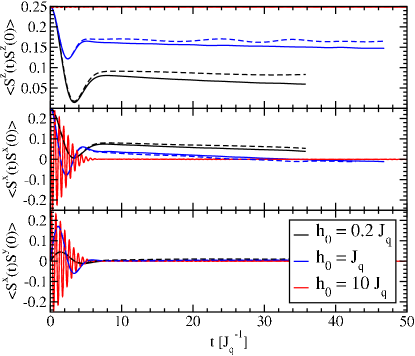
Figure 3: (Color online) Nonvanishing autocorrelations $\overline{S_{0}^{\alpha}(t)S^{\beta}_{0}(0)}$ of the central spin for $N=99$ bath spins and various strengths of the external magnetic field. The solid lines represent the solution of the semiclassical model “Langevin 1” while the dashed lines are the quantum results calculated with DMRG. The results are shown up to the time where the total discarded weight of the DMRG calculations exceeds $10\,\%$, cf. discussion in Sect. II.3. The semiclasscial simulation involved $M=100\,000$ random time series.

The semiclassical model (5) can also be used for finite external fields. For brevity, we restrict ourselves to the simple semiclassical model (5) (Langevin 1) without conservation of the total spin. The cases of a weak field $h_{0}=0.2\,J_{\mathrm{q}}$, an intermediate field $h_{0}=J_{\mathrm{q}}$, and a strong field $h_{0}=10\,J_{\mathrm{q}}$ applied to the central spin are investigated. In these cases, the mean value of the Gaussian fluctuations in $z$ direction acquires the role of the finite external field

$$\overline{\eta_{z}\left(t\right)} =h_{0},$$ (25)

while all other mean values remain zero. The nonvanishing correlation functions $\braket{A^{z}(t)A^{z}(0)}$, $\braket{A^{x}(t)A^{x}(0)}$, and $\braket{A^{x}(t)A^{y}(0)}$ of the Overhauser field are calculated with DMRG. The results are determined up to the time where the total discarded weight exceeds $10\,\%$. More details on the implied accuracy can be found in Sec. II.3. They serve as input for the cylindric correlation functions $g_{zz}(t)$, $g_{xx}(t)$, and $g_{xy}(t)$, respectively. The nonzero autocorrelations of the central spin are plotted in Fig. 3 for a bath of $N=99$ spins.

A very nice agreement between the semiclassical (solid lines in Fig. 3) and the quantum data (dashed lines) is found in the strong-field regime where the dynamics is dominated by the Larmor precession of the central spin. For low and intermediate fields, a certain mismatch between both descriptions is always present. In general, the quantum and the semiclassical approach agree remarkably well. Note that the discrepancies are more pronounced in the spin direction parallel to the external field than in the perpendicular direction.

We attribute the observed mismatch to the missing conservation of the total $z$ component of the spin. We refrain here from discussing the possible improvement by its inclusion because such calculations would still need the input of the bath correlations. Instead, we will show below that a completely classical simulation is more efficient and more reliable.

II.5 Limitations of the semiclassical approach

We achieved a significant improvement in the semiclassical description of the CSM by incorporating the conservation of the total spin explicitly. For finite external fields, the incorporation of the $z$ component of the total spin is not strictly required because a good agreement in spin directions perpendicular to the external field is already achieved without this conservation. However, two essential disadvantages of the semiclassical approach remain.

First, it relies on an additional method providing the correlations of the random noise of the Overhauser field. Hence, accessible time scales are limited by this additional method and almost no resources are saved.

Second, the semiclassical approach does not respect the energy conservation of the CSM

$$0 \stackrel{{\scriptstyle!}}{{=}}\frac{\mathrm{d}}{\mathrm{d}t}H_{\mathrm{sc}}=\frac{\mathrm{d}\vec{\eta}\left(t\right)}{\mathrm{d}t}\cdot\vec{S}_{0}\neq 0.$$ (26)

The energy is conserved in the quantum model where the state of the bath depends on the state of the central spin such that $H$ is constant. The relevant important backactions effects are not included in the semiclassical picture so that the energy conservation is lost. This may be repaired by some clever incorporation of the energy conservation in a similar way to what we did for the spin conservation. However, the task appears to be complicated and in view of the first, remaining caveat less attractive.

These considerations lead us to the next section, where a completely classical simulation is compared to the quantum-mechanical results.

III Classical Equations of Motion

In the previous section, we illustrated the importance of the proper treatment of conserved quantities. This conclusion is supported further by the rigorous bounds for the correlations of the central spin found very recently.Uhrig et al. (2014) Thus, searching for a computationally simple approach to the CSM it is natural to think of classical calculations Merkulov et al. (2002); Erlingsson and Nazarov (2004); Al-Hassanieh et al. (2006); Chen et al. (2007); Coish et al. (2007) because the classical model has the same conserved quantities as the quantum-mechanical one.

In addition, the norm of the commutators of the Overhauser field vanish relative to the norm of the Overhauser field itself for an infinite bath $N\to\infty$.Stanek et al. (2013) Note that in quantum dots $N$ is of the order of $10^{5}$. Thus it is well justified to treat the Overhauser field classically. We showed in the previous section that the dynamics of the central spin can also be determined by considering it as classical vector due to the linearity of the corresponding equations of motion. Only for the backaction of the central spin on the individual bath spins it is not evident if a classical treatment resembles the quantum-mechanical one.

A qualitative argument in favor of the agreement of the classical and the quantum-mechanical approach is the separation of time scales: the central spin precesses faster by a factor of about $\sqrt{N}$ than a single bath spin. So the single bath spin is exposed to a long-time average of the central-spin dynamics. Such an average is believed to behave classically.

It is the purpose of the present section to study quantitatively to what extent the quantum-mechanical dynamics and the classical one agree. The relevant classical $3(N+1)$ equations of motion (EOMs) read

$$\frac{\mathrm{d}}{\mathrm{d}t}\vec{S}_{0} =\vec{A}\times\vec{S}_{0}-\vec{h}_{0}\times\vec{S}_{0}$$ (27a)

$$\frac{\mathrm{d}}{\mathrm{d}t}\vec{S}_{i} =J_{i}\vec{S}_{0}\times\vec{S}_{i},$$ (27b)

where $i\in\left\{1,2,\ldots,N\right\}$ and $\vec{h}_{0}$ is the external field applied to the central spin. The classical Overhauser field is defined by

$$\vec{A} :=\sum\limits_{i=1}^{N}J_{i}\vec{S}_{i}.$$ (28)

The Overhauser field is a vector in $\mathds{R}^{3}$ and not an operator anymore as in the quantum model. The equations (27) are derived in Ref. Al-Hassanieh et al., 2006 as a time-dependent mean-field approximation to the quantum model.

It is easily verified that the total energy

$$E =\vec{A}\cdot\vec{S}_{0}$$ (29a)

$$\Rightarrow\frac{\mathrm{d}E}{\mathrm{d}t} =\left(\frac{\mathrm{d}\vec{A}}{\mathrm{d}t}\right)\cdot\vec{S}_{0}+\vec{A}\cdot\left(\frac{\mathrm{d}\vec{S}_{0}}{\mathrm{d}t}\right)=0$$ (29b)

is conserved because of the properties of the outer product.

The set (27) of coupled EOMs is solved best using standard numerical routines such as Runge-Kutta integration. Here, we stick to the adaptive Runge-Kutta-Fehlberg method which is part of the GNU Scientific Library (GSL).Galassi et al. (2009) As in Sect. II.2, the initial values for all spins $\vec{S}_{i}(t)$ at $t=0$ are chosen from a Gaussian distribution with vanishing mean value. The variance is given from the quantum-mechanical expectation values for disordered $S=1/2$:

$$\overline{S^{\alpha}_{i}(0)S^{\alpha}_{i}(0)} =\frac{1}{4}.$$ (30)

By the numerical integration, one obtains the time evolution of all spins $\vec{S}_{i}$. The desired autocorrelations of the central spin are calculated by averaging over a large number $M$ of random initial configurations. This corresponds to the investigation of a completely unpolarized system at infinite temperature. It would be straightforward to implement analogous calculations for (partially) polarized baths.

In our numerical implementation, we checked the conservation of the energy and of the total spin explicitly to verify the correctness of the code. The energy in the studied time interval $t\in[0,1000\,J_{\mathrm{q}}^{-1}]$ is conserved within $10^{-6}$, which also corresponds to the step size of the Runge-Kutta integration. On the same time scale, the total momentum is conserved within $10^{-12}$. Decreasing the step size of the Runge-Kutta method did not lead to a significant improvement so that we used $10^{-6}$ as standard value throughout.

III.1 Classical results for zero field

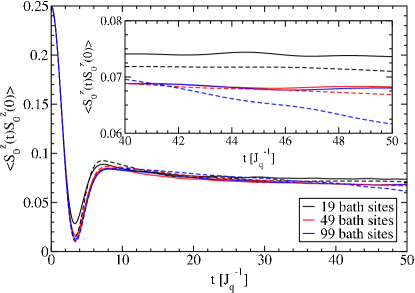
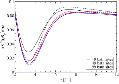
Figure 4: (Color online) (Top) Autocorrelation function of the central spin for zero field up to intermediate time scales. In addition to the classical solution (solid lines), the DMRG results of the corresponding quantum model are plotted (dashed lines). The inset displays a magnification for $t\geq 40\,J_{\mathrm{q}}^{-1}$. On these time scales, the DMRG result for $N=99$ appears to be slightly inaccurate, which we attribute to the total discarded weight. The results for the classical EOMs are averaged over $M=1\,000\,000$ random initial configurations of the spin vectors. The lower panel displays a magnification of the short-time behavior illustrating that the classical data and the quantum-mechanical DMRG data agree better and better for larger and larger spin baths.

At first, we study the case without external field. The results for the autocorrelation of the central spin are plotted in Fig. 4. Overall, the classical solutions (solid lines) and the DMRG results (dashed lines) agree nicely up to intermediate times $t=50\,J_{\mathrm{q}}^{-1}$. The minimum close to $t\approx 4\,J_{\mathrm{q}}^{-1}$ is not correctly captured by the classical solution if the bath size is small, cf. lower panel. However, fast convergence with $N$ is observed so that only a marginal difference between the classical and the quantum results remains for a moderate number of $N=99$ bath spins. Of course, an absolute agreement cannot be expected since both quantum and classical description are distinct. Hence the observed agreement between the two approaches is already remarkable.

After the plateau of the autocorrelation has emerged beyond $t\approx 7J_{\mathrm{q}}^{-1}$, a good agreement between classical and quantum results persists, in particular for larger spin baths. It supports the idea that the large number of interaction partners and the clear separation of energy scales makes the quantum dynamics very close to the classical one.

The drop in the DMRG result for $N=99$ bath spins beyond $t\geq 40\,J_{\mathrm{q}}^{-1}$ is to be attributed to numerical inaccuracies because the total discarded weight is close to 10% on the respective time scale. More details on accuracy can be found in Sect. II.3.

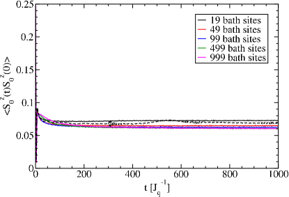
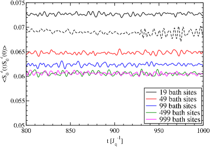
Figure 5: (Color online) (Top) Long-time behavior of the autocorrelation of the central spin obtained from the classical EOMs for up to $N=999$ bath spins. The lower panel displays a magnification for larger times $t\geq 800\,J_{\mathrm{q}}^{-1}$ where the curves fluctuate around a constant finite value. The black dashed curve is obtained from the Chebyshev expansion for $N=19$ bath spins.Hackmann (2013); Hackmann and Anders (2014) The results for the classical EOMs are averaged over $M=1\,000\,000$ random initial configurations of the spin vectors.

Next, we address the behavior at long times. The key problem is that we do not have reliable quantum data available for long times. A first impression is provided in Fig. 5 for a bath of $N=19$ spins for which times up to $t=1000J_{\mathrm{q}}^{-1}$ are accessible by the Chebyshev expansion.Hackmann and Anders (2014) Only bath sizes $\approx 20$ can be tackled by the Chebyshev expansion. For large values of $t$, all curves acquire a plateau value which depends on the actual bath size. The persisting plateau value is generally identified as the nondecaying fraction of the autocorrelation.Faribault and Schuricht (2013a, b) From the lower panel of Fig. 5, we see that the value of the nondecaying fraction converges well with diverging system size $N$. We recall that in real quantum dots the number of bath spins exceeds $10^{5}$ easily. By mathematically rigorous bounds the existence of nondecaying fractions has been established only recently for the quantum CSM, provided the mean coupling $\overline{J}:=\lim_{N\to\infty}N^{-1}\sum_{i=1}^{N}J_{i}$ does not vanish.Uhrig et al. (2014) Estimates of the nondecaying fractions for the classical CSM can be found in the literature.Merkulov et al. (2002); Chen et al. (2007)

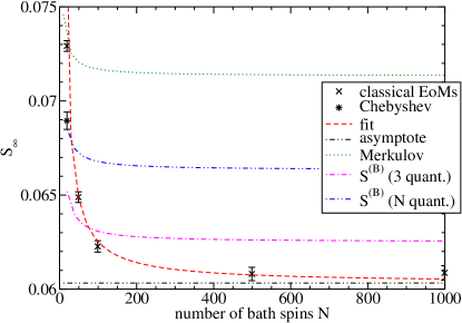
Figure 6: (Color online) Nondecaying fraction $S_{\infty}$ of the autocorrelation of the central spin (symbols) vs the number of bath spins $N$. The long-time results of the classical EOMs fluctuate around a constant value (see lower panel of Fig. 5)), the mean values for $t=500$–$1000\,J_{\mathrm{q}}^{-1}$ are plotted. The error bars depict the standard deviation. The red curve represents the fit function $f(N)=3a(N/b+1)/(N/b-1)$ with $a=0.0201$ and $b=1.79$. To show the asymptotics, we plot the $N=\infty$ limit $f(N)\xrightarrow{N\rightarrow\infty}3a$ as determined by the fit (blue curve). The dotted (green) curve depicts the estimate from Ref. Merkulov et al., 2002 for our set of coupling constants. In addition, the quantum-mechanical estimates for $S_{\infty}$ in the quantum model are depicted.Uhrig et al. (2014)

We want to elucidate the behavior of the nondecaying fraction resulting from our classical simulation and compare it with the quantum-mechanical estimates as they are provided by the formulas in Ref. Uhrig et al., 2014. This is done in Fig. 6 where we plot the numerically determined values $S_{\infty}$ for the nondecaying fraction, that is

$$S_{\infty} :=\overline{S^{z}_{0}(t\rightarrow\infty)S^{z}_{0}(0)}.$$ (31)

This quantity has been estimated by Merkulov et al. in Ref. Merkulov et al., 2002 by a formula that depends only on the following combination of the mean coupling $\overline{J}$ and the mean square coupling $\overline{J^{2}}$

$$\frac{\overline{J}^{2}}{\overline{J^{2}}-\overline{J}^{2}}=3\frac{N+1}{N-1}$$ (32)

where the right-hand side applies to the couplings (4) we are studying here. The formula of Merkulov et al. results are shown as the dotted (green) line in Fig. 6. It is clearly deviating from the numerical result by about 20%. By allowing the constants in (32) to vary, we introduce the fit function

$$f(N)=\frac{3a(N/b+1)}{N/b-1}$$ (33)

which describes the numerical data well, see the dashed (red) curve in Fig. 6, but it is of empirical value only.

Since we are ultimately interested in the comparison to the quantum case we include the quantum-mechanical estimates $S^{\textrm{(B)}}$ from Ref. Uhrig et al., 2014 which consider three or $N$ conserved quantities. Note the excellent agreement of the estimate from $N$ conserved quantities with the Chebyshev result for $N=19$ bath spins (star symbol). Thus, we assume that the estimate remains as close as this to the true nondecaying fraction. Then, we have to deduce that the classical simulation underestimates the quantum-mechanical result by about 10%. This is interesting because it is a priori unclear whether the classical correlation decays more or less than the quantum correlation. One would have thought that quantum fluctuations reduce a persisting correlation below the classical value. However, it seems that the classical phase space imposes less restrictions on the central-spin dynamics than the quantum-mechanical Hilbert space. Certainly, the quantitative comparison of the classical and the quantum-mechanical nondecaying fraction deserves further investigation.

Summarizing, the quantum-mechanical dynamics of the electron spin in zero magnetic field is almost quantitatively described by the classical simulation up to intermediate time scales. As a general trend, the agreement between quantum and classical dynamics improves upon increasing bath size.

On very long-time scale, the issue is not completely clear. Classical and quantum-mechanical results display a significant nondecaying fraction. There is evidence that the nondecaying fractions are larger in the quantum-mechanical CSM than in the classical CSM. So the entanglement between central spin and bath appears to protect the coherence, at least partially.

In essence, our observations agree with results by Coish et al..Coish et al. (2007) They compared the quantum solution with the corresponding classical solution for a single initial state and found that the dynamics is essentially classical up to a certain time. Beyond that time, quantum fluctuations have to be taken into account. However, they did not study the average over all initial conditions as we do. Furthermore, all couplings in their study were homogeneous $J_{i}=J$ and the expectation values of the observables were calculated on the mean-field level. A numerical solution of the full set of EOMs was not considered.

The classical equations of motion (22) can also be viewed as the equations for a time-dependent mean-field approximation.Al-Hassanieh et al. (2006) As such this approximation turns out to be fairly crude.Dobrovitski and De Raedt (2003); Al-Hassanieh et al. (2006) Thus, we conclude that the average over the manifold of classical trajectories must be the key improvement in our classical approach. The assumption to use Gaussian distributed random initial spin orientations which are compatible with the initial quantum-mechanical expectation values appears to be the appropriate choice.

Al-Hassanieh et al. also start from random initial spin orientations, which are compatible with the initial density matrix.Al-Hassanieh et al. (2006) In this respect, both approaches are similar. Then, however, they derive a set of differential equations for the approximate temporal evolution of the density matrix. Finally, this set is integrated to describe the dynamics of the central spin. The authors emphasize, that their approach does not amount up to the integration of semiclassical equations of motion. In contrast, we employ the classical equations of motion (22), but with suitably weighted averages over various initial conditions. The numerical effort required in both approaches appears to be very similar because finally, a set of ordinary differential equations has to be integrated over time. Their number is of the order of the number of spins considered.

III.2 Classical results for finite external field

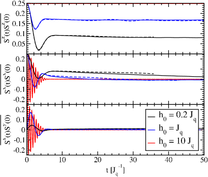
Figure 7: (Color online) Nonvanishing autocorrelations $\overline{S_{0}^{\alpha}(t)S^{\beta}_{0}(0)}$ of the central spin for $N=99$ bath spins and various strengths of the external magnetic field. The solid lines represent the classical simulation while the dashed lines are the quantum results calculated by DMRG. The latter are shown up to the time where the total discarded weight exceeds $10\,\%$. (The implied accuracy is discussed in detail in Sect. II.3.) Where they are not visible they lie underneath the classical curves. All classical curves are obtained by averaging over $M=1\,000\,000$ random initial configurations of the spin vectors.

In this section, we consider the classical simulations in presence of a finite external field. For simplicity, it is applied along the $z$ direction $\vec{h}_{0}=(0\ 0\ h_{0})^{\top}$. According to the EOMs in Eq. (27), the external field is solely applied to the central spin due to the three orders of magnitude between the electronic and the nuclear gyromagnetic ratio. As before, the case of a weak field $h_{0}=0.2\,J_{\mathrm{q}}$, an intermediate field $h_{0}=J_{\mathrm{q}}$, and a strong field $h_{0}=10\,J_{\mathrm{q}}$ is investigated. The following results comprise the behavior up to intermediate times. In Fig. 7, the nonvanishing autocorrelations of the central spin are plotted for the three regimes of the external field for a fixed bath size of $N=99$ spins. The solutions of the classical EOMs (solid lines) are compared to the behavior found in the quantum model (dashed lines of the same color/shading).

The essential dynamics of the central spin is captured by the classical EOMs. For weak and intermediate values of $h_{0}$, a noticeable influence of quantum fluctuations persists which leads to quantitative deviations between the classical and the DMRG results on intermediate time scales. Still, for large baths one observes qualitatively the same behavior. In the spin direction parallel to the external field, hardly any influence of the quantum fluctuations is discernible. Perpendicular to $h_{0}$, the classical autocorrelations decay slightly faster than their quantum counterparts.

We think that these findings imply that the very general argument based on spin path integrals that the classical behavior describes the quantum-mechanical one for large baths Chen et al. (2007) must be regarded with some caution. On the basis of our findings it is obvious that the agreement of both behaviors depends on the parameter regime, in particular on the size of the applied magnetic field. Thus we presume that the convergence of classical and quantum-mechanical regime is not uniform: up to a given time one can find a system size $N$ above which the classical and the quantum curves agree well. However, for small magnetic fields and for fixed system size $N$, there is a time beyond which both approaches behave differently.

Remarkably, for strong external field $h_{0}\gg J_{\mathrm{q}}$, the quantum and classical solutions cannot be distinguished. Generally, the classical EOMs indeed capture the crossover from the weak to the strong field regime visible in the DMRG data in Fig. 7. In the strong field regime, the dynamics in the central-spin model is classical as demonstrated in Fig. 8. Note as well that in this regime, the dependence on the number $N$ of bath spins is extremely weak, i.e., the convergence with system size is rapidly achieved. The dynamics is dominated by the Larmor precession induced by the strong external field.

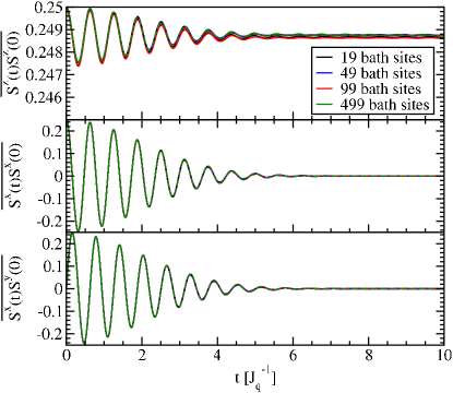
Figure 8: (Color online) Nonvanishing autocorrelation functions $\overline{S_{0}^{\alpha}(t)S^{\beta}_{0}(0)}$ of the central spin for a strong external field $h_{0}=10\,J_{\mathrm{q}}$. No longer times are depicted because no visible dynamics takes place beyond $t\approx 10J_{\mathrm{q}}^{-1}$. The solid lines represent the solution of the classical EOMs while the dashed lines are the quantum results calculated with DMRG. All classical curves are obtained by averaging over $M=1\,000\,000$ random initial configurations of the spin vectors.

We point out that DMRG also exhibits an extremely good performance in the strong field regime: the external field suppresses the relaxation of the central spin, i.e., its entanglement with the bath degrees of freedom. Hence, the number of important states to be kept by the DMRG increases significantly more slowly with $t$ than for low or zero magnetic field. This implies an important reduction of the total discarded weight at fixed number of kept states. In consequence, the code runs faster and/or much larger times can be reached. This can be made quantitative by the small total discarded weight which does not exceed $\mathcal{O}(10^{-4}$–$10^{-3})$ even on long time scales $t\approx 100J_{\mathrm{q}}^{-1}$. On the methodological level, this is a key observation for the use of DMRG in the description of qubits.

At this stage, we are in the position to address one of the essential question of spin decoherence. We consider the standard relaxation times. The so-called spin-lattice relaxation time $T_{1}$ quantifies the longitudinal relaxation parallel to the external field. From Fig. 8, it is obvious that no substantial longitudinal relaxation takes place, see the scale of the uppermost panel depicting the $S^{z}S^{z}$ correlation. Thus $T_{1}=\infty$ holds for the CSM in a sufficiently strong magnetic field.

The so-called spin-spin relaxation time $T_{2}$ quantifies the transversal dephasing. We determine it from a fit of the function

$$\braket{S^{x}_{0}(t)S^{x}_{0}(0)} =\frac{1}{4}\cos\left(\omega t\right)\operatorname{e}^{-\frac{t^{2}}{2T_{2}^{2}}}$$ (34)

to the DMRG data or to the classical data. We refrain from a detailed analysis for intermediate or weak fields so that both the quantum and the classical approach serve the purpose equally well. In the following, we use the DMRG results for $N=499$ bath spins as input. The extracted dephasing times $T_{2}$ are plotted in Fig. 9 up to very large values of $h_{0}$. The value $h_{0}=2\,J_{\mathrm{q}}$ is the lowest magnetic field for which a fit of the DMRG data to Eq. (34) works reasonably well.

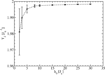
Figure 9: Spin-spin relaxation (or dephasing) time $T_{2}$ as a function of the external magnetic field $h_{0}$. The values for $T_{2}$ are obtained by fitting the function defined in Eq. (34) to the DMRG autocorrelation $\braket{S^{x}_{0}(t)S^{x}_{0}(0)}$ for $N=499$ bath spins. The error bars represent the errors of the fit. Note the small scale of the $T_{2}$-axis.

As indicated by the small error bars, the function defined in Eq. (34) approximates the autocorrelation function $\braket{S^{x}_{0}(t)S^{x}_{0}(0)}$ for $h_{0}>5\,J_{\mathrm{q}}$ extremely well. The error of the fit increases for smaller values of $h_{0}$ where Eq. (34) starts to deviate from the temporal behavior of the autocorrelation $\braket{S^{x}_{0}(t)S^{x}_{0}(0)}$. However, with respect to the very small scale of the $T_{2}$-axis in Fig. 9, we conclude that $T_{2}$ hardly depends on $h_{0}$. This finding establishes that the dephasing time $T_{2}$ is solely determined by the intrinsic time scale $J_{\mathrm{q}}^{-1}$ of the hyperfine interaction. The external field $h_{0}$ does not have any influence on the dephasing time $T_{2}$ once it is sufficiently large, $h_{0}\gtrapprox 2J_{\mathrm{q}}^{-1}$. This finding agrees perfectly with the line width and shape of the autocorrelation spectrum of the central spin, which was found to be essentially independent on a sufficiently large magnetic field for large magnetic field Hackmann and Anders (2014)

Many further studies of related Hamiltonians are called for at this stage. For instance, the investigation of the dependence of $T_{2}$ on various distributions of couplings suggests itself. Similarly, various extensions by additional couplings such as quadrupolar interactions for larger spins Sinitsyn et al. (2012) or dipole-dipole couplings Merkulov et al. (2002) between the bath spins will help to understand the spin dynamics in quantum dots quantitatively.

IV Conclusion

The goal of the present paper was twofold. First, we aimed at establishing efficient methods to compute the dynamics of the central spin in the central-spin model (CSM). Second, on the conceptual level, we provided strong evidence that the correct treatment of conserved quantities is important. This applies, in particular, to the total spin and the total energy.

We studied a semiclassical, Langevin type approach to the central-spin dynamics and a classical simulation for it. To verify the agreement of these descriptions with the full quantum-mechanical ones, we compared their results to the quantum results obtained from the previously introduced DMRG approach.Friedrich (2006); Stanek et al. (2013)

For the simple semiclassical model (Langevin 1), it turned out that the results deviate rather quickly from the quantum CSM. The explicit incorporation of conserved quantities such as the total spin improved the agreement of the semiclassical model (Langevin 2 or 3) with the quantum result substantially for zero magnetic field. Still, this approach does not conserve the total energy because no backaction effects from the central spin on the bath are incorporated. Additionally, on the technical level, it is a major caveat that the bath fluctuations have to be known from an additional, external source.

Neither restriction holds for the fully classical simulation based on the solution of the classical equations of motion for both, the central spin and the bath spins. The classical model shares the same conserved quantities with the quantum CSM.Gaudin (1983); Chen et al. (2007) Clearly, no further input from other sources is required. We found that the agreement of the classical ansatz with the quantum results depends on the strength of the external field applied to the central spin. We could not establish classical behavior for large $N$ independent of the considered time $t$ and of further parameters such as the magnetic field as suggested by a spin path integral argument.Chen et al. (2007) Without external field or for small fields, quantum fluctuations induce a quantitative deviation between the classical and the quantum model. For large fields, i.e., about twice the size of the root-mean-square of the Overhauser field, the classical simulations agree very well with the quantum results. We emphasize that in this regime the DMRG also works extremely well and can access long times.

By either the DMRG or the classical calculation we determined the relaxation rates $1/T_{1}$ and $1/T_{2}$ in the regime of strong fields. The spin-lattice relaxation rate is essentially zero while the spin-spin relaxation rate is given by $\approx J_{\mathrm{q}}$ independent of the magnetic field as long as it is strong enough.

Future application of the semiclassical, the classical approach or the full quantum-mechanical DMRG to the central-spin model comprise the simulation of coherent control pulses and trains of such pulses which extend the dephasing time of the central spin. Furthermore, the model can be extended by passing to larger spins, adding anisotropic couplings such as quadrupolar terms, or by including dipole-dipole interactions between the bath spins. In this way, the understanding of the dynamics of electron spins in quantum dots can be put on a more and more quantitative basis.