Magnetohydrodynamic Viscous Flow Over a Shrinking Sheet With Second Order Slip Flow Model

Abstract

In this paper, we investigate the magnetohydrodynamic viscous flow with second order slip flow model over a permeable shrinking surface. We have obtained the closed form of exact solution of Navier-Stokes equations by using similarity variable technique. The effects of slip, suction and magnetic parameter have been investigated in detail. The results show that there are two solution branches, namely lower and upper solution branch. The behavior of velocity and shear stress profiles for different values of slip, suction and magnetic parameters has been discussed through graphs.

Keywords: Navier-Stokes equations; MHD Viscous flow; Similarity Solution.

1 Introduction

The fluid flow due to a moving boundary has a great important in the expulsion processes [1]-[3]. The boundary layer on a stretching surface with a constant speed has been studied first time by Sakiadis [4, 5]. Later on Wang [6] pointed out that solution presented by Sakiadis was not an exact solution of Navier-Stokes solutions. The exact solution of two dimensional Navier-Stokes equations over a stretching sheet sheet was presented by Crane [7]. Gupta and Gupta [8], have examined the effect of mass transfer on Crane flow. For three dimensional background, the stretching sheet problem was investigated by Wang [9]. In this paper, the exact similarity solutions of Navier-Stokes equations were obtained. This study was extended to the rotating flow over double stretchable disks [10]. All these solutions are exact solutions of the Navier-Stokes equations.

The magnetohydrodynamic (MHD) flow over a stretching sheet was studied extensively [11]-[14] in the recent years, for both impermeable surface and permeable surface. The micro-scale fluid dynamics in the Micro-Electro-Mechanical Systems has received a considerable interest in among the researchers. The flow of such fluids belongs to the slip flow regime, which is entirely different from the traditional flow [15]. For the flow in the slip regime, the fluid flow obeys the Navier Stokes equations in the presence of slip velocity or temperature boundary conditions. In addition, partial velocity slips over a moving surface occur for particular fluids such as emulsions, suspensions and polymer solutions [16].

The slip flows under different flow configurations have been investigated by various authors [17]-[22]. With a slip at the wall boundary, the flow behavior with slip conditions are different from no-slip conditions. Among these studied, Andersson [17] and [18] investigated the slip flow over an impermeable stretching surface. In a recent paper, Wang [22] examined the mass transfer effects on the slip flow over a stretching surface. However, there was no study on the slip MHD flow over a permeable stretching surface in the literature. Fang et al.[23] studied study the first order slip MHD flow over a permeable stretching surface. Exact solutions of the governing Navier-Stokes equations were presented. Also, Fung et al.[24] studied the viscous flow over a shrinking sheet with second order slip flow model. However, there was no study on MHD viscous flow over a shrinking sheet with second order slip flow model. Therefore, the objective of the current paper is to study the second order slip MHD flow over a permeable shrinking surface. Exact solutions of the governing Navier-Stokes equations are presented and discussed in detail.

2 Mathematical Formulation and Solution of Problem

We consider two dimensional laminar flow of magnetized viscous fluid over a continuously shrinking sheet. The shrinking velocity of the sheet is $U_{w}=-U_{0}x$, where $U_{0}$ is a constant and $v_{w}=v_{w}(x)$ is wall mass transfer velocity. The x-axis is along the shrinking surface in the direction opposite the sheet motion and y-axis is perpendicular to it. By these assumptions the corresponding Navier-Stoke’s equations for the present problem can be summarized by the following set of equations [13]-[15], [19, 20]:

$$\frac{\partial u}{\partial x}+\frac{\partial u}{\partial y}=0;$$ (2)

$$u\frac{\partial u}{\partial x}+v\frac{\partial u}{\partial y}=-\frac{1}{\rho}\frac{\partial p}{\partial x}+\nu(\frac{\partial^{2}u}{\partial x^{2}}+\frac{\partial^{2}u}{\partial y^{2}})-\frac{\sigma B^{2}u}{\rho},$$

$$u\frac{\partial v}{\partial x}+v\frac{\partial v}{\partial y}=-\frac{1}{\rho}\frac{\partial p}{\partial x}+\nu(\frac{\partial^{2}v}{\partial x^{2}}+\frac{\partial^{2}v}{\partial y^{2}}).$$ (3)

The boundary conditions [24] are

$$u(x,0)=U_{0}(x)+U_{slip},v(x,0)=v_{w},u(x,1)=0.$$ (4)

where $u$ and $v$ are the components of velocity in the $x$ and $y$ directions respectively, $\nu$ is the kinematic viscosity, $p$ is the fluid pressure, $\rho$ is fluid density and $U_{slip}$ is second order velocity slip which is valid for any arbitrary Knudsen numbers, $K_{n}$ [25] and is given by

$$U_{slip} = \frac{2}{3}\left(\frac{3-\alpha l^{3}}{\alpha}+\frac{3}{2}(\frac{1-\dot{l}^{2}}{K_{n}})\right)\lambda\frac{\partial u}{\partial y}-\frac{1}{4}\left(l^{4}+\frac{2}{{K_{n}}^{2}}(1-l^{2})\right){\lambda}^{2}\frac{\partial^{2}u}{\partial y^{2}}$$ (5)

$$= A\frac{\partial u}{\partial y}+B\frac{\partial^{2}u}{\partial y^{2}}$$

where $l=min\left[\frac{1}{K_{n}}-1\right]$, $0\leq\alpha\leq 1$ is the momentum accommodation coefficient and $\lambda>0$ is the molecular mean free path. According to the definition of $l$, it is observed that $0\leq l\leq 1$, for any value of $K_{n}$. The stream function and similarity variable would be of the following form

$$\psi(x,y)=f(\eta)x\sqrt{vU_{0}},~{}~{}~{}\eta(x,y)=y\sqrt{\frac{U_{0}}{v}}.$$ (6)

With these definitions the components of velocities are

$$u=f^{\prime}(\eta)xU_{0},~{}~{}v=-f(\eta)\sqrt{vU_{0}}.$$ (7)

The wall mass transfer velocity becomes

$$v_{w}=f(0)\sqrt{vU_{0}}.$$ (8)

Using Eqs.(7) and (8) in (3)

$$\frac{p}{\rho}=\nu\frac{\partial v}{\partial y}-\frac{v^{2}}{2}+constant$$ (9)

Also, by using Eqs.(7)-(9) in Eq.(2), we obtain

$$f^{\prime\prime\prime}+ff^{\prime\prime}-{f^{\prime}}^{2}-M^{2}f^{\prime}=0,$$ (10)

where $M^{2}=\frac{\sigma B^{2}}{\rho\mu_{0}}$. The boundary conditions are

$$f^{\prime}(0)=-1+\gamma f^{\prime\prime}(0)+\delta f^{\prime\prime\prime}(0),$$ (11)

$$f(0)=s$$ (12)

$$f^{\prime}(1)=0$$ (13)

where $s$ is the mass transfer parameter, $\gamma$ is the first order velocity slip parameter with $\gamma=A\sqrt{\frac{U_{0}}{\nu}}$ and $\delta=\frac{BU_{0}}{\nu}<0$ is the second order velocity slip parameter. The pressure term can be obtained from Eq.(9). In this section, we are interested to find the closed form of exact solution of Eq.(10) subjected to boundary conditions (11)-(13).

We assume the solution of the form

$$f(\eta)=a+be^{-\beta\eta}$$ (14)

Using above equation in the boundary condition (12), we get

$$s=a+b.$$ (15)

Equation (11) leads to

$$b=\frac{1}{\beta+\gamma{\beta}^{2}-\delta{\beta}^{3}}.$$ (16)

From Eqs.(15) and (16), we get

$$a=s-\frac{1}{\beta+\gamma{\beta}^{2}-\delta{\beta}^{3}}.$$ (17)

Using the values of $a$ and $b$ in the assumed solution (14), we get

$$f(\eta)=s-\frac{1}{\beta+\gamma{\beta}^{2}-\delta{\beta}^{3}}+\frac{1}{\beta+\gamma{\beta}^{2}-\delta{\beta}^{3}}e^{-\beta\eta}.$$ (18)

The use of this relationship in Eq.(10), leads to the following fourth order algebraic equation for $\beta$

$$\beta^{4}+A_{3}{\beta}^{3}+A_{2}\beta^{2}+A_{1}\beta+A_{0}=0;$$ (19)

where

$$A_{3}=\frac{-\gamma-\delta s}{\delta},~{}~{}A_{2}=\frac{\gamma s-\delta M^{2}-1}{\delta},~{}~{}A_{1}=\frac{s+\gamma M^{2}}{\delta},~{}~{}A_{0}=\frac{M^{2}-1}{\delta}.$$ (20)

Now our focus is to find the solution of above equation, such solution can be determined by wall mass transfer $s$, first order slip parameter $\gamma$ and second order slip parameter $\delta$ . The only positive roots of Eq.(19) are solutions. By defining $z=\beta+\frac{A_{3}}{4}$, Eq.(19) can be converted to following standard form

$$z^{4}+P{z}^{2}+qz+r=0,$$ (21)

where

$$P=A_{2}+\frac{3}{8}{A_{3}}^{2},~{}~{}q=A_{1}-\frac{1}{2}A_{2}A_{3}+\frac{1}{8}{A_{3}}^{3},$$

$$r=A_{0}-\frac{1}{4}A_{1}{A_{3}}+\frac{1}{16}A_{2}{A_{3}}^{2}-\frac{3}{256}{A_{3}}^{4}.$$ (22)

Mathematically, there are four roots of Eq.(21), real roots of this equation can be written explicitly in the following form

$$\beta_{1}=\frac{\sqrt{c}}{2}-\frac{1}{2}\sqrt{D-\frac{2q}{\sqrt{c}}}-A_{3}$$

$$\beta_{2}=\frac{\sqrt{c}}{2}+\frac{1}{2}\sqrt{D-\frac{2q}{\sqrt{c}}}-A_{3},$$ (23)

where

$$c= \frac{-2P}{3}+\frac{2^{\frac{1}{3}}(P^{2}+12r)}{\left(3(2P^{2}+27q^{2}-72Pr+\sqrt{-4(P^{2}+12r)^{3}+(2P^{2}+27q^{2}-72Pr)^{2})}^{\frac{1}{3}}\right)}$$

$$+ \frac{\left(3\left(2P^{2}+27q^{2}-72Pr+\sqrt{-4(P^{2}+12r)^{3}+(2P^{2}+27q^{2}-72Pr)^{2}}\right)^{\frac{1}{3}}\right)}{3\times 2^{\frac{1}{3}}}$$

$$D= \frac{-4P}{3}-\frac{2^{\frac{1}{3}}(P^{2}+12r)}{\left(3(2P^{2}+27q^{2}-72Pr+\sqrt{-4(P^{2}+12r)^{3}+(2P^{2}+27q^{2}-72Pr)^{2})}^{\frac{1}{3}}\right)}$$

$$+ \frac{\left(3\left(2P^{2}+27q^{2}-72Pr+\sqrt{-4(P^{2}+12r)^{3}+(2P^{2}+27q^{2}-72Pr)^{2}}\right)^{\frac{1}{3}}\right)}{3\times 2^{\frac{1}{3}}}$$

Here $\beta_{1}$ and $\beta_{2}$ corresponds to lower and upper branch solution, respectively.

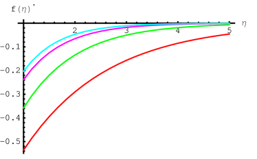
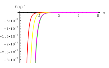
Figure 1: The left and right figures describe the behavior of $f^{\prime}(\eta)$ corresponding to lower and upper branch solution, respectively for varying $\gamma$ and $s=1,~{}\delta=-0.01,~{}M=0.1.$ In the left figure light green, pink, green and red curves corresponds to $\gamma=0.08,~{}0.04,~{}0.01,~{}0.1,$ respectively while in right figure red, brown, pink and green curves correspond to $\gamma=0.08,~{}0.04,~{}0.01,~{}0.1,$ respectively.

To show the effects of slip and magnetic parameters on the fluid flow, we present the velocity and shear stress profiles for different combinations of $M,~{}\delta,~{}\gamma$ and $s$. The velocity profile is presented in figures 1-4. The left graph in figure 1 shows that for lower branch solution the velocity of the shrinking sheet increases with the increase of $\gamma$ by keeping all the other parameters fixed. The right graph in figure 1 shows that for upper branch solution the velocity of the shrinking sheet increases from $-\infty$ value to zero, with the increase of $\gamma$. The similar behavior of velocity profile is depicted in the both graphs of figure 2 for lower and upper branch solutions, respectively, with varying $s$.

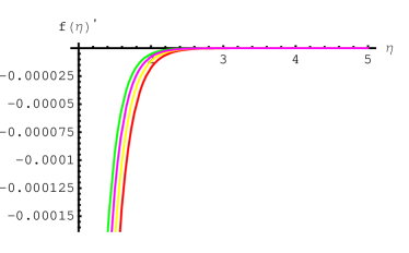
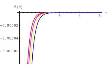
Figure 2: The left and right figures describe the behavior of $f^{\prime}(\eta)$ corresponding to lower and upper branch solution, respectively for varying $s$ and $\gamma=0.1,~{}\delta=-0.01,~{}M=0.1.$ In the left figure red, brown, pink and green curves corresponds to $s=0.1,~{}0.2,~{}0.3,~{}0.4,$ respectively while in right figure blue, brown, pink and red curves correspond to $s=0.1,~{}0.2,~{}0.3,~{}0.4,$respectively.

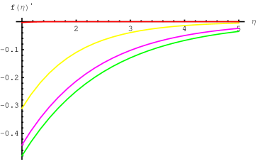
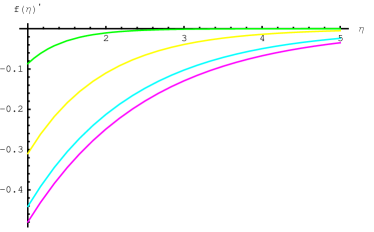
Figure 3: The left and right figures describe the behavior of $f^{\prime}(\eta)$ corresponding to lower and upper branch solutions, respectively for varying $M$ and $\gamma=0.1,~{}\delta=-0.01,~{}s=1.$ In the left figure red, brown, pink and green curves corresponds to $M=0.1,~{}2,~{}3,~{}4,$ respectively while in right figure green, brown, light green and pink curves correspond to $M=0.1,~{}2,~{}3,~{}4,$ respectively.

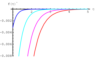
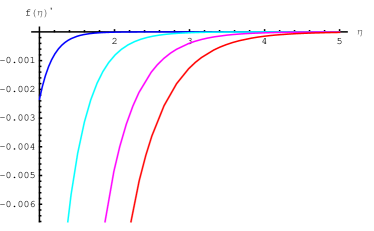
Figure 4: The left and right figures describe the behavior of $f^{\prime}(\eta)$ corresponding to lower and upper branch solution, respectively for varying $\delta$ and $\gamma=0.1,~{}s=1,~{}M=0.1.$ In both figures the blue, light green, pink and red curves corresponds to $\delta=-0.01,~{}-0.02,~{}-0.03~{}-0.04,$ respectively.

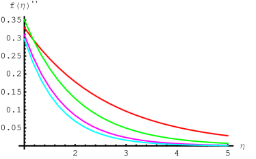
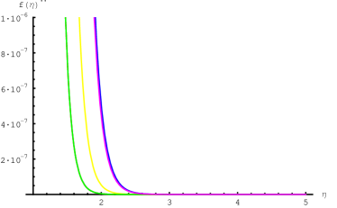
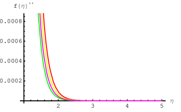
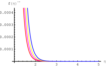
Figure 5: The left and right figures describe the behavior of $f^{\prime\prime}(\eta)$ corresponding to lower and upper branch solutions, respectively for varying $\gamma$ and $s=1,~{}\delta=-0.01,~{}M=0.1$. In the left figure light green, pink, green and red curves correspond to $\gamma=0.04,~{}0.02,~{}0.01,~{}0.1,$ respectively while in right g- ure blue, pink, brown and green curves correspond to $\gamma=0.04,~{}0.02,~{}0.01,~{}0.1,$ respectively.

Figure 6: The left and right figures describe the behavior of $f^{\prime\prime}(\eta)$ corresponding to lower and upper branch solutions, respectively for varying $s$ and $\gamma=0.1,~{}\delta=-0.01,~{}M=0.1$. In the left figure red, brown, pink and green curves corresponds to $s=0.1,~{}0.2,~{}0.3,~{}0.4,$ respectively while in right figure blue, brown, pink and red curves correspond to $s=0.1,~{}0.2,~{}0.3,~{}0.4,$ respectively.

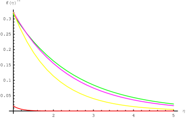
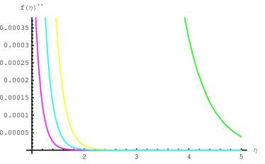
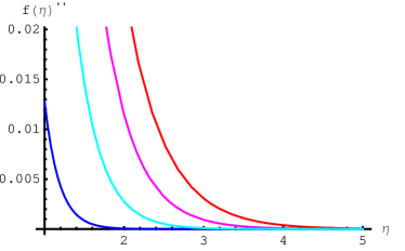
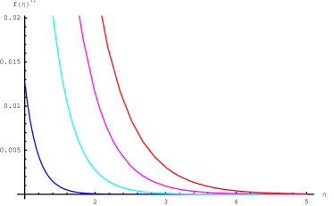
Figure 7: The left and right gures describe the behavior of $f^{\prime\prime}(\eta)$ corresponding to lower and upper branch solution, respectively for varying $M$ and $s=1$,$\delta=-0.01,~{}\gamma=0.1$. In the left figure red, brown, pink and green curves correspond to $M=0.1,~{}1,~{}2,~{}3,$ respectively while in right figure green, brown, light green and pink curves correspond to $M=0.1,~{}1,~{}2,~{}3,$ respectively.

Figure 8: The left and right figures describe the behavior of $f^{\prime\prime}(\eta)$ corresponding to lower and upper branch solutions, respectively for varying $delta$ and $s=1,~{}M=0.1,~{}\gamma=0.1$. In both figures the blue, light green, pink and red curves corresponds to $\delta=-0.01,-0.02,0.-03,-0.04,$ respectively.

The left graph in the figure 3 shows that for lower branch solution the velocity of the shrinking sheet increase of $\delta$. For maximum value of $\delta=-0.01$, velocity reduces from negative finite values to zero. All the remaining curves imply that a sheet moving with infinite velocity is highly damped due to magnetohydrodynamical effects. The same behavior of the velocity profile appear in case of upper branch solution with varying $\delta$ is shown in right graph of figure 3. In figure 4 the lower and upper branch solution for the velocity of the shrinking sheet have been plotted with varying $M$, respectively. In left graph of figure 4 for small magnetic effect velocity is always zero while all the others curves implies that shrinking sheet moving with finite velocity either comes to rest or moves with constant velocity as it becomes parallel to $\eta$-axis.

The shear stress of the wall is shown in figures 5-8. The left graph in figure 5 shows that in case of lower branch solution wall stress decreases with the increase of slip parameter $\gamma$. The wall stress decreases as sheet moves with maximum speed. Similar behavior of shear stress with increasing $\gamma$ is presented in right graph of figure 5 for upper branch solution. All the stress profiles have same nature for the variation of different parameters. From the both graphs in figure 7, it can be deduced that shearing stress on the wall is linearly related to the strength of magnetic field.

3 Conclusion

In this paper, we have investigated the exact solution of governing Navier-Stokes equations for the magnetohydrodynamic viscous flow over a shrinking sheet with second order slip. We have examined the effect of slip parameters, magnetic parameters suction parameter on the fluid flow. We have presented the velocity profile $f^{\prime}(\eta)$ and wall stress profile $f^{\prime\prime}(\eta)$, for the different combination $M,~{}\delta,~{}\gamma$ and $s$. It has been found that the effect of $\delta<0$ (due to shrinking sheet) on velocity and shear stress profiles in upper and lower branch solutions case is same. An interesting feature appear, when M is small stress is small and velocity is zero. In case of varying $\delta$, velocity is highly damped due to magnetic effects.

References

• [1] Altan, T., Oh, S. and Gegel, H. Metal forming fundamentals and applications. Metals Park: American Society of Metals; 1979.
• [2] Fisher, E.G. Extrusion of plastics. New York: Wiley; 1976.
• [3] Tadmor, Z. and Klein, I. Engineering principles of plasticating extrusion. Polymer science and engineering series. New York: Van Nostrand Reinhold; 1970.
• [4] Sakiadis, B.C. Boundary-layer behavior on continuous solid surface: I. Boundary-layer equations for two-dimensional and axisymmetric flow. J. AIChe 7(1961)26.
• [5] Sakiadis B.C. Boundary-layer behavior on continuous solid surface: II. Boundary-layer equations for two-dimensional and axisymmetric flow. J. AIChe 7(1961)221.
• [6] Wang, C.Y. Exact solutions of the steady state Navier Stokes equations. Ann. Rev. Fluid Mech. 23(1991)159.
• [7] Crane, L.J. Flow past a stretching plate. Z Angew Math. Phys. 21(1970)645.
• [8] Gupta, P.S. and Gupta, A.S. Heat and mass transfer on a stretching sheet with suction or blowing. Can. J. Chem. Eng. 55(1977)744.
• [9] Wang, C.Y. The three-dimensional flow due to a stretching flat surface. Phys. Fluids 27(1984)1915.
• [10] Fang, T. and Zhang, J. Flow between two stretchable disks an exact solution of the Navier Stokes equations. Int. Commun. Heat Mass Transfer 35(2008)892.
• [11] Chakrabarti A, Gupta AS. Hydromagnetic flow and heat transfer over a stretching sheet. Quart. Appl. Math. 37(1979)73.
• [12] Andersson, H.I. An exact solution of the Navier Stokes equations for magnetohydrodynamic flow. Acta. Mech. 113(1995)241.
• [13] Pop, I. and Na, T.Y. A note on MHD flow over a stretching permeable surface. Mech. Res Commun. 25(1998)263.
• [14] Liao, S.J. On the analytic solution of magnetohydrodynamic flows of non-Newtonian fluids over a stretching sheet. J. Fluid Mech. 488(2003)189.
• [15] Gal-el-Hak, M. The fluid mechanics of microdevices The Freeman Scholar Lecture. J. Fluids Eng. Trans. ASME 121(1999)5.
• [16] Yoshimura, A., Prudhomme, R.K. Wall slip corrections for Couette and parallel disc viscometers. J. Rheol. 32(1988)53.
• [17] Andersson, H.I. Slip flow past a stretching surface. Acta Mech. 158(2002)121.
• [18] Wang, C.Y. Flow due to a stretching boundary with partial slip an exact solution of the Navier Stokes equations. Chem. Eng. Sci. 57(2002)3745.
• [19] Fang, T., Lee, C.F. Exact solutions of incompressible Couette flow with porous walls for slightly rarefied gases. Heat Mass Transfer 42(2006)255.
• [20] Wang, C.Y. Stagnation slip flow and heat transfer on a moving plate. Chem. Eng. Sci. 61(2006)7668.
• [21] Wang, C.Y. Stagnation flow on a cylinder with partial slip an exact solution of the Navier Stokes equations. IMA J. Appl. Math. 72(2007)271.
• [22] Wang, C.Y. Analysis of viscous flow due to a stretching sheet with surface slip and suction. Nonlinear Anal. Real World Appl. 10(2009)375.
• [23] Fang, T., Zhong, J. and Shanshan, Y. Slip MHD viscous flow over a stretching sheet An exact solution. Commun. Nonlinear Sci. Numer. Simulat. 14(2009)3731.
• [24] Fang, T., Shanshan, Y., Zhong, J. and Aziz, A. Viscous flow over a shrinking sheet with second order flow slip model. Commun. Nonlinear Sci. Numer. Simulat. 15(2010)1831.
• [25] Wu, L. A slip model for rarefied gas flows at arbitrary Knudsen number. App. Phys. Lett. 93(2008)253.