Low-mass galaxy formation and the ionizing photon budget during reionization

Abstract

We use high-resolution simulations of cosmological volumes to model galaxy formation at high-redshift, with the goal of studying the photon budget for reionization. We demonstrate that galaxy formation models that include a strong, thermally coupled supernovae scheme reproduce current observations of star formation rates and specific star formation rates, both during and after the reionization era. These models produce enough UV photons to sustain reionization at $z{\la}8$ ($z{\la}6$) through a significant population of faint, unobserved, galaxies for an assumed escape fraction of 20% (5%). This predicted population is consistent with extrapolation of the faint end of observed UV luminosity functions. We find that heating from a global UV/X-ray background after reionization causes a dip in the total global star formation rate density in galaxies below the current observational threshold. Finally, while the currently observed specific star formation rates are incapable of differentiating between supernovae feedback models, sufficiently deep observations will be able to use this diagnostic in the future to investigate galaxy formation at high-redshift.

1 Introduction

Understanding the Epoch of reionization, in which a primarily neutral Universe underwent a phase transition to an almost completely ionized intergalactic medium (IGM) is a key driver in numerous theoretical and observational projects. This transition is a challenge to study observationally due to the faintness of the sources responsible for reionization, and because they are obscured by the neutral medium at optical wavelengths. It is also a challenge to theoretically model this epoch through supercomputer simulations due to the enormous dynamic range between the small physical scales of the sources and the large volumes they affect. It is clear that the process of reionization is all but complete by redshift $z{\sim}6$ due to the presence of the Gunn & Peterson (1965) trough in quasar spectra at higher redshifts (e.g. Fan et al., 2006). Observations of cosmic microwave background (CMB) photons (Hinshaw et al., 2013) are consistent with an instantaneous reionization model that occurs at $z{=}10.3\pm 1.1$, implying that a more realistic ‘extended’ reionization was well underway by this time.

Table 1: A list of the simulated galaxy formation physics schemes utilized in this study. From left to right, the columns list the simulation name used in this study, the name as defined by Schaye et al. (2010) where appropriate (else ‘–’ used to indicate a new scheme), and a brief the description of the physics modelled. Each of these simulations has been run twice to test the effects of reionization on early galaxy formation. When we add the label LateRe (EarlyRe) to the simulations names below we have modelled an instantaneous reionization at $z_{\rm r}{=}6.5$ $(9)$ with a Haardt & Madau (2001) UV/X-ray background thereafter (see Section 4.1 for more details).

Simulation	OWLS name	Brief description
PrimC_NoSNe	NOSN_NOZCOOL	No energy feedback from SNe and cooling assumes primordial abundances
PrimC_WSNe_Kinetic	NOZCOOL	Cooling as PrimC_NoSNe but with fixed mass loading of ‘kinetic’ winds from SNe
ZC_WSNe_Kinetic	REF	SNe feedback as PrimC_WSNe_Kinetic but now cooling rates include metal-line emission
ZC_SSNe_Kinetic	–	Strong SNe feedback as ZC_WSNe_Kinetic but using 100% of available SNe energy
ZC_SSNe_Thermal	WTHERMAL	Strong SNe feedback as ZC_SSNe_Kinetic but feedback ‘thermally’ coupled

Recent ultra deep observations using the Hubble Space Telescope (HST) have begun constraining the galaxy UV luminosity function during the heart of this reionization era at $z{\sim}7-8$ (e.g. Bouwens et al., 2011a; Schenker et al., 2013; McLure et al., 2013). Robertson et al. (2013) extrapolated the observed luminosity functions four magnitudes deeper than the Hubble Space Telescope Ultra Deep Field (HUDF) limits (Ellis et al., 2013; Koekemoer et al., 2013) and found that these faint objects could sustain reionization given reasonable assumptions for the number of ionizing photons from the galaxies and clumping factor of the IGM. In this work, we demonstrate that this extrapolation is supported by our simulated galaxy populations, which exhibit a rising luminosity function below the observational magnitude limits that is sufficient to reionize the universe by $z{\la}8$.

As well as constraining luminosity functions, observations are also beginning to probe the nature of galaxies at high-redshifts. In particular, galaxies at higher redshifts have a higher specific star formation rate (sSFR; e.g. Stark et al., 2013). This had been predicted theoretically (e.g. Bouché et al., 2010; Davé et al., 2011a) but was in disagreement with observations at the time which found a rapid rise in the sSFR from today to $z{\sim}2$ and then little or no evolution at higher redshift (e.g. Daddi et al., 2007; Noeske et al., 2007; Stark et al., 2009; González et al., 2010). We discuss this result in the light of different models of supernovae (SNe) feedback in this work. We find that current surveys have little discriminating power, but that deeper observations can strongly discriminate between the feedback models, and determine the approximate redshift of reionization, through a combination of SFR and sSFR measurements.

The rest of this paper is organised as follows. In Section 2 we introduce the new simulation suite Smaug and the range of galaxy formation physics we have examined. We then discuss the physics driving the SFR function (Section 3) and the sSFR (Section 3.2). We show in Section 4 that our simulations support the paradigm of a ‘Photon-Starved’ Epoch of reionization (Bolton & Haehnelt, 2007), in which the number of ionizing photons is only just sufficient to sustain global reionization. In Section 5, we demonstrate that there exists a faint galaxy population below observational limits that is consistent with extrapolating recent luminosity functions. We conclude in Section 6.

2 Simulation Details

We have created a suite of high-resolution, cosmological volume hydrodynamical simulations, named Smaug, as part of the Dark Ages reionization and Galaxy Formation Simulations project (DRAGONS). The Smaug series of simulations all share the same initial conditions, i.e. are identical simulation volumes, but are resimulated using a number of different physics models (selected as a subset from the OverWhelmingly Large Simulations series OWLS; Schaye et al. 2010) which allows robust testing of the relative impact that each galaxy physics component has on observables such as SFRs for example. These physics models have seen a number of successes in reproducing observed galaxy properties at low, post-reionization, redshifts. For example, the cosmic star formation history (SFH; e.g. Madau et al., 1996) was shown to be reproduced in Schaye et al. (2010), as well as the high-mass end of the Hi  mass function in Duffy et al. (2012).

The Smaug simulations were run with an updated version of the publicly available Gadget-2 $N$-body/hydrodynamics code (Springel, 2005) with new modules for radiative cooling (Wiersma et al., 2009a), star formation (Schaye & Dalla Vecchia, 2008), stellar evolution and mass-loss (Wiersma et al., 2009b) and galactic winds driven by SNe (Dalla Vecchia & Schaye, 2008, 2012). Each simulation employed $N^{3}$ dark matter (DM) particles, and $N^{3}$ gas particles, where $N{=}512$ for the production runs presented here (lower resolution test cases with $N{=}128$ and $256$ were also run for extensive resolution testing, see Duffy et al. in preparation) within cubic volumes of comoving length $L{=}10\,h^{-1}{\rm Mpc}$. The Plummer-equivalent comoving softening length is $200\,h^{-1}{\rm pc}$ and the DM (gas/star) particle mass is $4.7\,(0.9)\times 10^{5}\,h^{-1}{\rm M_{\odot}}$ respectively, for the $N{=}512$ production runs. For all cases, we used grid-based cosmological initial conditions generated with GRAFIC (Bertschinger, 2001) at $z{=}199$ using the Zeldovich approximation and a transfer function from COSMICS (Bertschinger, 1995).

We use the Wilkinson Microwave Anisotropy Probe 7-year results (Komatsu et al., 2011), henceforth known as WMAP7, to set the cosmological parameters $[\Omega_{\rm m},$ $\Omega_{\rm b},$ $\Omega_{\Lambda},$ $h,$ $\sigma_{8},$ $n_{\rm s}]$ to [0.275, 0.0458, 0.725, 0.702, 0.816, 0.968] and $f^{\rm univ}_{\rm b}{=}0.167$.

2.1 Galaxy Formation Physics

The naming convention for the simulations follows that of Duffy et al. (2010), with PrimC indicating that only cooling from primordial elements (i.e. hydrogen and helium) is included. With simulations named ZC we have included metal line emission cooling from hydrogen, helium and nine elements: carbon, nitrogen, oxygen, neon, magnesium, silicon, sulphur, calcium and iron (calculated from the photoionization package CLOUDY, last described in Ferland et al. 1998).

For the high-redshift simulations presented in this work, we have focused on testing the role of SNe feedback on early galaxy formation including the effects of metals realized by these events enhancing the cooling rates of gas. We run a number of these models, from the same initial condition, but systematically increasing the complexity of the models to test the relative impact of the galaxy physics in observables such as SFR. Our first simulation is the most simplistic model possible, that of primordial gas cooling (PrimC) that can then form stellar populations without a resultant phase of SNe feedback (NoSNe). This first case is referred to as PrimC_NoSNe and results in runaway star formation as expected.

We then consider the cases where the SNe is able to couple a fraction of the available energy to nearby gas. The label WSNe refers to weak feedback SNe (i.e. 40% of the available SNe energy is coupled) and SSNe refers to strong (i.e. 100% available SNe energy coupled). There are two main techniques to couple this energy. The first uses SNe energy to heat nearby gas particles and to allow an outflow to build from the resultant overpressurized gas (Dalla Vecchia & Schaye, 2012). We term this Thermal feedback. The alternative is to skip straight to the ‘snowplough’ phase of the SNe feedback and directly ‘kick’ gas particles (Dalla Vecchia & Schaye, 2008) which we call Kinetic feedback.

Due to radiative losses, the Kinetic feedback will have only a fraction of the available SNe energy $f_{\rm SNe}$ coupled into driving a wind (i.e. ‘kicking’ the gas particles in this case), while the Thermal scheme implicitly models these losses (Dalla Vecchia & Schaye, 2012) and hence is modelled using a higher fraction of the SNe energy ($f_{\rm SNe}{=}0.4,\,1.0$ respectively). To test if differences between the Kinetic and Thermal models was a result of numerical modelling, or simply the different fraction of SNe energy used, we also ran a maximal ‘strong’ Kinetic scheme with $f_{\rm SNe}{=}1.0$, in Duffy et al. (in preparation). We found that this ‘strong’ Kinetic scheme was in excellent agreement with the Thermal model, indicating our resolution is sufficiently high that the method of coupling to the gas is not as important as the amount of energy released. Therefore, although for completeness we have included ZC_SSNe_Kinetic in Table 1 it is effectively indistinguishable from ZC_SSNe_Thermal in the plots shown in this work and hence is not included for clarity.

The assumed initial mass function (IMF) for star formation in the Smaug simulation series is from Chabrier (2003). When comparing with observational works which use the Salpeter (1955) IMF we reduce their SFR and stellar masses by a factor $1.65$. This reduction has been shown by Haas et al. (2013) to adequately address the conversion from UV photon counts from massive stars using the two IMFs.

The stellar feedback schemes we consider in this work are in good agreement with observed stellar mass functions and sSFRs at $z{=}0-2$ (Haas et al., 2013) at higher mass scales (their fig 4). These are therefore a compelling subset of simulations to consider at higher redshift. We refer the reader to Duffy et al. (2010) and Schaye et al. (2010) for further details of the simulations. We provide a summary of the naming convention in Table 1. In a future work, we will examine the impact that changing star formation prescriptions have on high-redshift galaxy formation. In this work, we have focused predominantly on the role that feedback plays for these objects.

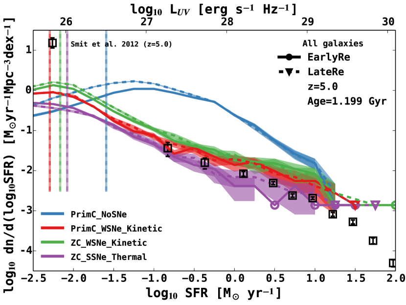
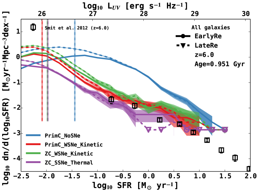
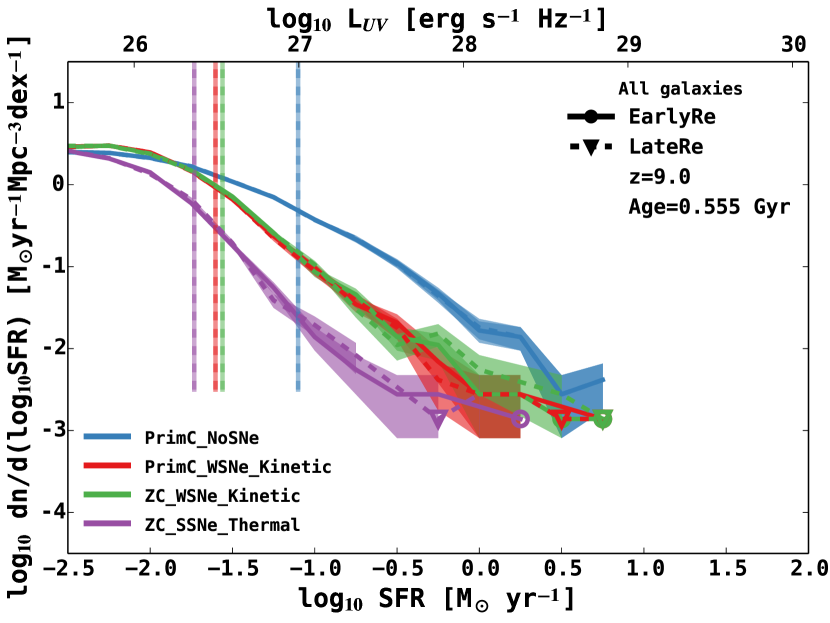
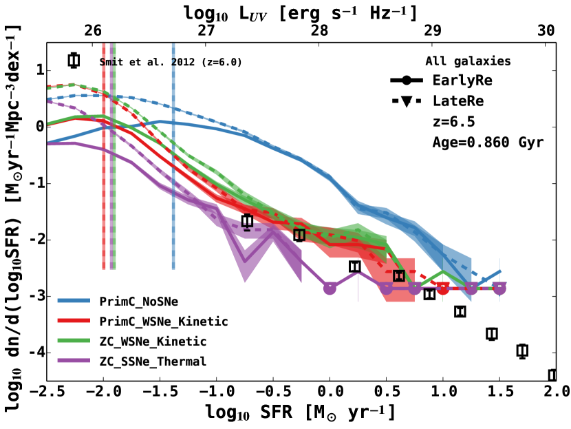
Figure 1: The SFRD at $z{\sim}5.0,\,6.0,\,6.5,\,9.0$ (top left clockwise) for different simulations, errors are Poissonian and indicated by the faint band around each of the curves. Typically for galaxies with high (${>}10\,\rm M_{\odot}\rm{yr}^{-1}$) SFR, there is only one object in the binning range which we represent with a circle (down triangle) for early (late) reionization models. The galaxies at the very highest (${>}30\,\rm M_{\odot}\rm{yr}^{-1}$) SFR are mergers. The solid (dashed) curves are the models with an instantaneous reionization at $z_{\rm r}{=}9$ ($6.5$), while the colours represent the different simulation physics runs; PrimC meaning primordial cooling only, ZC means metal lines can contribute to the cooling rate too. NoSNe is no feedback, WSNe is the weak kinetic feedback, SSNe is the strong thermal feedback. The shaded regions are $1\sigma$ confidence limits estimated by bootstrap. The observations in open squares are from Smit (private communication) who applied the methodology of Smit et al. (2012) with dust-corrections of Bouwens et al. (2013) to the latest rest-frame UV continuum observations of galaxies from Bouwens et al. (2014). We then corrected the SFR to a Chabrier (2003) IMF. The vertical lines are the approximate resolution limits of the simulations, below which the SFR will be increasingly underestimated.

.

2.2 Implementation of reionization

The effect of reionization is to suppress the contribution of faint end galaxies through photoevaporation of the gas as well as prevention of further accretion from the IGM (e.g. Shapiro et al., 2004; Iliev et al., 2005). To test the impact of reionization in our simulations we ran two different sets of models. In one case we assumed an early ($z_{\rm r}{=}9$) reionization (labelled EarlyRe) and the other a late ($z_{\rm r}{=}6.5$) reionization (labelled LateRe). These redshifts are reasonable bracketing cases from CMB and Lyman $\alpha$ forest bounds, e.g. Fig. 12 of Pritchard et al. (2010). Following Pawlik et al. (2009) and Schaye et al. (2010), we model reionization as an instantaneous event across the box, which is appropriate for the small volume of our simulation which would lie within a single Hii  region during reionization (Furlanetto et al., 2004).

At reionization, all gas is exposed to a uniform Haardt & Madau (2001) UV/X-ray background. We do not model radiative transfer in this work and instead calculate photoheating rates in the optically thin limit. At reionization, this will lead to an underestimate of the IGM temperature (e.g. Abel & Haehnelt, 1999) and we follow Pawlik et al. (2009) and Wiersma et al. (2009a) by injecting 2eV per proton of additional thermal energy to ensure the gas is heated to $T{=}10^{4}\rm K$. After reionization ($z{<}z_{\rm r}$) all cooling rates are calculated in the presence of the evolving photoionizing Haardt & Madau (2001) UV/X-ray background, as given in Wiersma et al. (2009a). For redshifts higher than $z{=}9$ the cooling rates are calculated in the presence of both the CMB and photodissociation from the $z{=}9$ background (as Haardt & Madau 2001 did not tabulate for $z{>}9$) with a cutoff in the spectrum above 1 Ryd. This ‘softer’ background will suppress the formation of molecular hydrogen by the first stars/ionizing sources (Pawlik et al., 2009).

3 Origin of UV Photons

In this section we consider the galaxy formation physics that is required to match the distribution of SFRs (the SFR function, Section 3.1), and the efficiency of star formation (i.e. sSFRs, Section 3.2).

3.1 SFR function

We first compare the SFR density (SFRD) function of the models with observational results from Smit (private communication) who applied the methodology of Smit et al. (2012), and the dust-corrections of Bouwens et al. (2013), to the latest rest-frame UV continuum observations of galaxies from Bouwens et al. (2014) using HST data in the HUDF09 and CANDELS fields (Grogin et al., 2011; Koekemoer et al., 2011; Bouwens et al., 2012a). The quoted errors do not include the uncertainties due to imperfect dust-corrections and hence discrepancies between simulation and observations are likely less severe than they appear. In Fig. 1, we show the observations and the simulation results for representative redshifts at $z{\sim}5,\,6,\,6.5,\,9$ (top left clockwise).

Broadly speaking, the simulations that include feedback are in good agreement with observations below $10\,\rm M_{\odot}\rm{yr}^{-1}$ at all redshifts (a similar result at larger mass scales has also been seen in Tescari et al. 2014). The thermal SNe scheme (ZC_SSNe_Thermal; purple curve) is able to match the SFRD function at $z{\sim}5-6$ (top panels of Fig. 1). Although at $z{\sim}6.5$ this model slightly underproduces the number of objects with SFR ${\sim}1\,\rm M_{\odot}\rm{yr}^{-1}$ from Smit (private communication).

At the very highest SFRs (${>}30\,\rm M_{\odot}\rm{yr}^{-1}$), the abundance of objects appears to be strongly overestimated in the simulations irrespective of the galaxy formation physics considered. In practice, within each SFR bin there is only one galaxy, indicated with a point and no errors (Poissonian error would be unity), and the last two data points at $z=5$ for the very highest rates are a result of an ongoing merger. In a small simulation, volume statistics are limited for the highest SFRs and they will suffer from cosmic variance, $\sigma_{\rm V}$. To estimate how significant these simulated outliers are from the observed SFR function we use Somerville et al. (2004) to estimate $\sigma_{\rm V}{=}b\sigma_{\rm DM}$, where $b$ is bias of the population and $\sigma_{\rm DM}$ the variance of the underlying DM halo. The highest SFR of $\sim 50\,\rm M_{\odot}\rm{yr}^{-1}$ at $z=5$ is in a halo of mass $2.86\times 10^{11}\,h^{-1}{\rm M_{\odot}}$, which is calculated (Pontzen et al., 2013) to have a bias $b=6.5$. From Somerville et al. (2004) we have $\sigma_{\rm DM}{\sim}0.3$ for our boxsize, giving $\sigma_{\rm V}{=}b\sigma_{\rm DM}{=}1.8$, which makes the final data points highly susceptible to cosmic variance and thus disagreements with the observations are of negligible statistical significance. Why the merger triggered starbursts are visible in the simulations so often is suggestive that we are lacking an additional suppression of star formation in the largest systems, perhaps through supermassive black hole feedback (e.g. Booth & Schaye, 2009). We will test the impact of supermassive black holes on the galaxy properties in future work but caution that in the limited cosmological volume of our simulations we wouldn’t expect to find quasars of significant black hole mass (from McGreer et al. 2013 a single object of mass ${\sim}10^{9}\,\rm M_{\odot}$ would be found in a $\rm Gpc$ volume).

Finally, we caution that the observations may be underestimating the bright end of the SFRD function due to imperfect dust extinction corrections which become ever more significant for galaxies with large SFR and/or stellar masses (e.g. Meurer et al., 1999; Santini et al., 2014). Indeed, just such a rise in the abundance of bright end galaxies has been seen in Bowler et al. (2014) using additional data from UltraVISTA (Bowler et al., 2012; McCracken et al., 2012). However, as argued by Wyithe et al. (2011), the exponential decline in the bright end of the luminosity function at $z{>}6$ is expected to disappear for galaxies ${<}-22$ mag due to gravitational lensing, which produces an observed power law luminosity function at bright luminosities (Pei, 1995). Due to the difficulties in uncovering the underlying luminosity function, as well as the lack of the most massive galaxies in the limited volume we simulate, we defer this analysis to a future, larger volume hydrodynamic simulation.

The simulations show the effect of radiative suppression of the low-mass (and low-SFR) galaxies by reionization (comparing the two bottom panels of Fig. 1, before and after the early reionization scheme has occurred). However, the effects of reionization become visible in objects with SFRs an order of magnitude below the observational results of Smit (private communication) shown in the bottom right panel of Fig. 1.

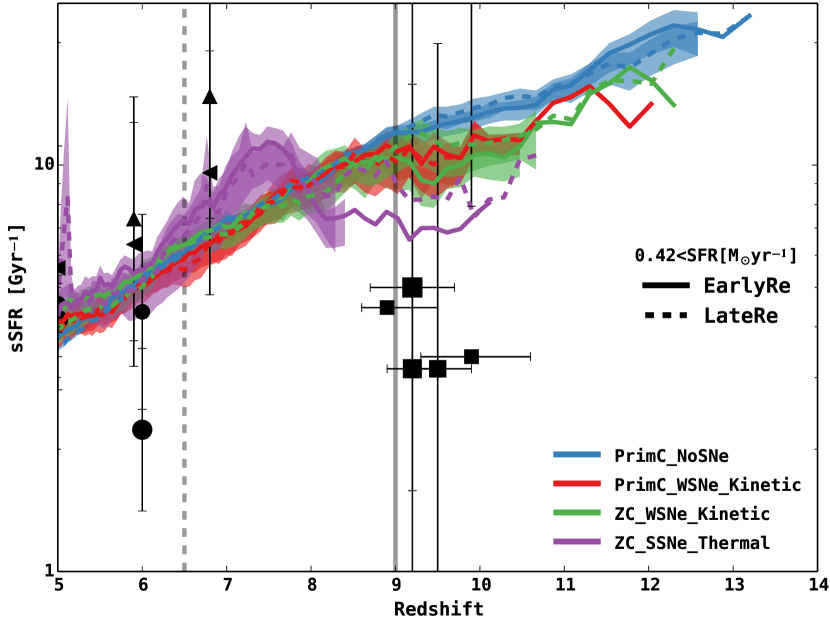
Figure 2: The sSFR rates as a function of redshift are now restricted for galaxies with an observationally derived cut of SFR $0.42\,\rm M_{\odot}yr^{-1}$ (corrected to our Chabrier IMF from the quoted limit of $0.7$ using the Salpeter IMF). The solid (dashed) curves are the models with an instantaneous reionization at ${z_{\rm r}}{=}9$ ($6.5$), while the colours represent the different simulation physics runs; PrimC meaning primordial cooling only, ZC means metal lines can contributed to the cooling rate too. NoSNe is no feedback, WSNe is the weak kinetic feedback, SSNe is the strong thermal feedback. The shaded regions are $1\sigma$ confidence limits estimated by bootstrap. The observations in black filled circles are from González et al. (2014) using a Constant SFH with nebulae emission line contaminations (and the point size represents the two stellar mass bins of $0.3$ dex, centred at $\log_{10}M_{*}\,h^{-1}{\rm M_{\odot}}{\approx}9.0$ and $9.7$); the black squares are the single galaxy observations from Oesch et al. (2014) and Holwerda et al. (2014), the triangles are from Stark et al. (2013) who corrected Bouwens et al. (2012b) stellar masses for contamination by nebulae emission lines; the leftward (upward) pointing triangles are assuming a fixed (evolving) H$\alpha$ equivalent width. The main result is that, surprisingly, the entire simulation series match the observations. As discussed in the text, this is a simple result of the observational limit imposed on the simulations.

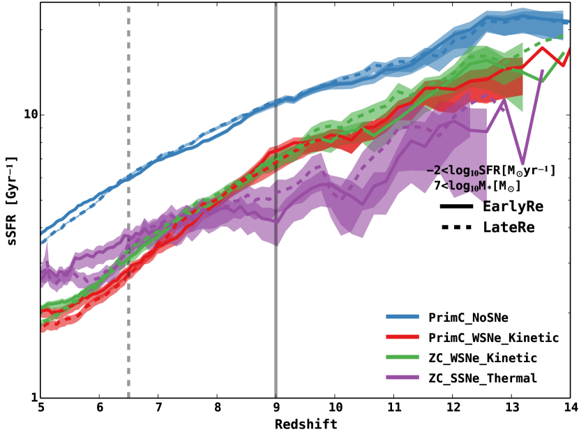
Figure 3: As in Fig. 2, we show the sSFR as a function of redshift, for all objects above the resolution limit of the simulation as determined in Duffy et al. (in preparation) this is an SFR 40 times below the observational cut and a stellar mass at least two orders of magnitude below the limits of González et al. (2014). The shaded regions are $1\sigma$ confidence limits estimated by bootstrap. We now see that the behaviour of the sSFR is a complex function of SNe feedback (sSFR is inversely proportional to increased feedback efficiency) , metal pollution of the IGM (resulting in enhanced cooling rates, and hence sSFR) and radiative feedback from reionization (typically a reduction of a factor of 5 in the sSFR). In particular, the timing of reionization results in a lasting impact on the sSFR, as described in the text. We have removed the observations shown in Fig. 2 as they correspond to a different selection effect than the one considered in this figure. However, to guide the relative change in the simulated sSFR we note that the blue PrimC_NoSNe model is essentially equivalent in this figure and Fig. 2.

3.2 Efficiency of star formation

The sSFR, along with the SFR, is a key variable observed at high-redshift. It is also an important prediction for infall-governed galaxy growth models which predict a rising sSFR with increasing redshift (e.g. Bouché et al., 2010; Davé et al., 2011a). In particular, Haas et al. (2013) found that the sSFR as a function of stellar mass was sensitive to the feedback model (their fig. 4, bottom-left panel) with a complex relation between sSFR and increasing stellar mass.

We emulate this test through first comparing the global sSFR with observations, and then extending the simulated sSFR measure to a minimum stellar mass. We note that in the near future there is unlikely to be sufficient observations available to construct the full differential plot, i.e. sSFR versus $M_{\star}$, although future observations (utilizing gravitational lensing) may be possible. Indeed, until recently most observations showed a rapid rise in the global sSFR from the present day to $z{\sim}2$ and then a plateau to higher redshifts (e.g. Daddi et al., 2007; Noeske et al., 2007; Stark et al., 2009; González et al., 2010). This picture has changed with the demonstration in de Barros et al. (2014) that nebular line emission could contaminate the stellar mass estimates, and the most recent observations of Stark et al. (2013) with this correction now demonstrate a continuing modest rise in sSFR for $z{>}4$. The observed sSFR is shown in Fig. 2 for galaxies with a minimum SFR of $0.42\,\rm M_{\odot}yr^{-1}$. The observational limits as given in Oesch et al. 2012 are $0.7\,\rm M_{\odot}yr^{-1}$, which we reduce by a factor of 1.65 to account for the different stellar initial mass function assumed, as argued by Haas et al. (2013). Note that we do not ‘correct’ the sSFR as both SFR and stellar mass are reduced by the same factor and hence cancel out to first order.

For comparison, in Fig. 2 we show that the Smaug simulations reproduce these observations, irrespective of reionization history or feedback scheme. We find that the sSFR in galaxies with SFR ${>}0.42\,\rm M_{\odot}yr^{-1}$ increases from $5\,[\rm Gyr^{-1}]$ at $z{=}5$ to ${\sim}10\,\rm Gyr^{-1}$ by $z{\sim}9$, in particular for the case of the no-feedback model (NoSNe in blue) ultimately reaching ${\sim}20\,\rm Gyr^{-1}$ by $z{\sim}12$. These values are in good agreement with a recent simulation by Dayal et al. (2013); however as we have tested a range of physics schemes we see that this matching is irrespective of the galaxy formation physics modelled, and should not be considered a ‘success’ of any one model. As discussed in Davé et al. (2011b) for models without feedback (NoSNe in blue), the only physics to impact the evolution of the sSFR is the accretion rate of material on to the growing haloes. For those simulations with stellar feedback, Davé et al. (2011b) argue that the insensitivity is due to the fact that the SN suppression of the SFR and growth in the stellar mass is reduced by a similar factor, meaning that the ratio of the quantities is unchanged. Therefore, we argue that this insensitivity (and the ability to match observations) is a direct result of the observational limit imposed on the simulated data.

Fig. 3 shows the predicted sSFR in galaxies with SFR ${>}0.01$ and $M_{\star}{>}10^{7}\,\rm M_{\odot}yr^{-1}$. These plots indicate that in a much deeper survey we would expect to be able to differentiate between feedback schemes, as they modify the typical star formation efficiency at lower galaxy stellar mass than currently observed. The global results shown in Fig. 3 demonstrate three key behaviours:

• The overall sSFR is reduced as feedback efficiency is increased (from no-feedback, weak and ultimately strong SNe feedback; blue, red and purple curves respectively) in agreement with, for example, Davé et al. (2011a). At early times, $z=10$, there is a simple scaling between sSFR and SNe energy fraction $f_{\rm SNe}$ used in the simulation; $sSFR\approx 13/(1+f_{\rm SNe})\,{\rm Gyr^{-1}}$ where $f_{\rm SNe}$ is $0$ for NoSNe, $0.4$ for WSNe and SSNe is $1$.

• Pollution of the IGM by metals enhances the cooling rate, and results in a small ${\sim}20\%$ increase in the sSFR (in qualitative agreement with Haas et al., 2013). This increase occurs with a small delay (i.e. becoming apparent only below $z=8$) as it takes time for significant amounts of metals to be produced and released (comparing PrimC and ZC models; green and red curves respectively).

• There is a modest hysteresis in the sSFR as to when reionization occurred. The stellar mass in the denominator of sSFR is an integral of the SFR, meaning that the instantaneous SFR is reduced just after reionization, while the stellar mass is approximately the same as a run with a different reionization redshift. This effect is an $\sim 5-10\%$ reduction in the sSFR (comparing purple curves dashed and solid line of ZC_SSNe_Thermal in Fig. 3) which is still visible at the end of the simulation. This memory is in contrast with the global SFR alone which quickly converges after reionization and the models of different reionization redshifts converge by $z{\sim}5$ as shown in 4 and Fig. 5).

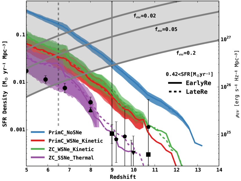
Figure 4: The Madau diagram (SFRD as a function of redshift) is presented with an observational cut of SFR $0.7\,\rm M_{\odot}yr^{-1}$ (converted to the Chabrier IMF this is $0.42$). The simulation which uses all of the available SNe energy (ZC_SSNe_Thermal) to drive an outflow, together with the observationally inferred cut, is in excellent agreement with the observations. The solid (dashed) curves are the models with an instantaneous reionization at $z_{\rm r}{=}9$ ($6.5$), while the colours represent the different simulation physics runs; PrimC meaning primordial cooling only, ZC means metal lines can contribute to the cooling rate too. NoSNe is no feedback, WSNe is the weak kinetic feedback, SSNe is the strong thermal feedback. The shaded regions are $1\sigma$ confidence limits estimated by bootstrap. The observations in black filled circles are based on the HUDF (Bouwens et al., 2007, 2011b; Oesch et al., 2012), the squares are the HUDF and eXtreme Deep Field with GOODS-South (Oesch et al., 2013), the pentagon is from HUDF and eXtreme Deep Field with both GOODS-South and North (Oesch et al., 2014), the upward pointing triangle is from BoRG (Bradley et al., 2012; Schmidt et al., 2014) and the downward pointing triangle is from CLASH (Bouwens et al., 2012a; Zheng et al., 2012; Coe et al., 2013). The bottom grey horizontal curve indicates the UV ionisation density to completely reionize the Universe (hence case ‘A’ recombination rates for hydrogen are used), assuming a clumping factor of 3 (Pawlik et al., 2009; Shull et al., 2012), escape fraction of $0.2$ (Ouchi et al., 2009) and a (logarithmic) ratio of Lyman continuum photons to UV flux of $25.2$ (Robertson et al., 2013). The other grey curves are for lower escape fractions.

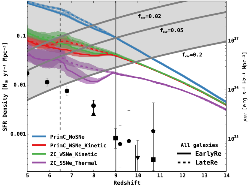
Figure 5: As with Fig 4 we show the Madau diagram but now with the observationally motivated limit on SFR relaxed to include all galaxies in the simulation. The solid (dashed) curves are the models with an instantaneous reionization at $z_{\rm r}{=}9$ ($6.5$), while the colours represent the different galaxy physics considered; PrimC meaning primordial cooling only, ZC means metal lines can contributed to the cooling rate too. NoSNe is no feedback, WSNe is the weak kinetic feedback, SSNe is the strong thermal feedback. The shaded regions are $1\sigma$ confidence limits estimated by bootstrap. The observations in black filled circles are based on the HUDF (Bouwens et al., 2007, 2011b; Oesch et al., 2012), the squares are the HUDF and eXtreme Deep Field with GOODS-South (Oesch et al., 2013), the pentagon is from HUDF and eXtreme Deep Field with both GOODS-South and North (Oesch et al., 2014), the upward pointing triangle is from BoRG (Bradley et al., 2012; Schmidt et al., 2014) and the downward pointing triangle is from CLASH (Bouwens et al., 2012a; Zheng et al., 2012; Coe et al., 2013). The grey horizontal curves indicates the UV ionisation density needed to completely reionize the Universe (hence case ‘A’ recombination rates for hydrogen are used), assuming a clumping factor of 3 (Pawlik et al., 2009; Shull et al., 2012), a plausible range of escape fraction (Wyithe et al., 2010) and a (logarithmic) ratio of Lyman continuum photons to UV flux of $25.2$ (Robertson et al., 2013).

Figure 6: As with Fig. 5 we show the Madau diagram with the observationally motivated limit on SFR relaxed to include all galaxies in the simulation, now focusing on the observability of the reionization ‘dip’, and hence the redshift range has been restricted. The solid (dashed) curves are the models with an instantaneous reionization at $z_{\rm r}{=}9$ ($6.5$), while the colours and represent the different galaxy physics considered; PrimC meaning primordial cooling only, ZC means metal lines can contribute to the cooling rate too. NoSNe is no feedback, WSNe is the weak kinetic feedback, SSNe is the strong thermal feedback. The shaded regions are $1\sigma$ confidence limits estimated by bootstrap. The grey horizontal curves indicates the UV ionisation density needed to completely reionize the Universe (hence, case ‘A’ recombination rates for hydrogen are used), assuming a clumping factor of 3 (Pawlik et al., 2009), a plausible range of escape fraction (Wyithe et al., 2010) and a (logarithmic) ratio of Lyman continuum photons to UV flux of $25.2$ (Robertson et al., 2013). We have applied a Gaussian weighted average across the lines with a $\sigma$ of $\Delta z{\approx}1$ to account for the variance in reionization due to the limited volume simulated. The sharp ‘dip’ seen in Fig. 5 is now a more gradual feature as the data is averaged over a larger redshift range. The error bars are also averaged in this measurement though and the ‘dip’ between schemes with early and late reionization remains easily discernible.

4 Sustaining reionization

In Fig 4, we show the global SFRD as a function of redshift (also known as a Madau diagram) for our models. To compare the simulation SFR with observations which measure UV luminosity, we have made use of the conversion between UV luminosity and SFR given by Robertson et al. (2013)

$$L_{\rm UV}\approx 1.25\times 10^{28}\times\frac{\rm{SFR}}{\,\rm M_{\odot}\rm{yr}^{-1}}{\rm erg\,s^{-1}\,Hz^{-1}}\,$$ (1)

which is valid for a Chabrier (2003) IMF at solar metallicity (using a constant SFR Bruzual & Charlot 2003 model). In addition we incorporate the observational limits of inferred global measurements, using a stated SFR limit of $0.7\,\rm M_{\odot}yr^{-1}$ from Oesch et al. (2012); they assume a Salpeter (1955) IMF which, when converted to a Chabrier (2003) IMF, corresponds to $0.42\,\rm M_{\odot}yr^{-1}$. In Fig. 4 we see that all simulation schemes show a rising SFRD with time, but separate out depending on the level of SNe feedback. In particular, our strongest SNe feedback model (ZC_SSNe; in purple) reproduces the observations at all redshifts.

For comparison, the grey curves indicate the level of SFRD (i.e. UV flux density) needed to sustain reionization at a given redshift, for a set of assumed escape fractions, $f_{\rm esc}$ (the fraction of ionizing photons produced by stars that can escape their galaxy and participate in ionizing the IGM). We calculate this UV density by solving for the evolution of the volume filling fraction of ionized hydrogen $Q_{{H{\sc ii}\,\,}}$. This is a balance between a ‘source’, the density of ionizing UV photons $\dot{n}_{\rm ion}$, and ’sinks’, recombinations in gas of density $\bar{n}_{\rm H}$ at a volume averaged recombination time $t_{\rm rec}$ (Madau et al., 1998)

$$\dot{Q}_{{H{\sc ii}\,\,}}=\frac{\dot{n}_{\rm ion}}{\bar{n}_{\rm H}}-\frac{Q_{{H{\sc ii}\,\,}}}{\bar{t}_{\rm rec}}\,.$$ (2)

At the completion of reionization, this equation simplifies to the steady state result of $\dot{Q}_{{H{\sc ii}\,\,}}{=}0$ and $Q_{{H{\sc ii}\,\,}}{=}1$ such that the ionizing photon density needed to sustain reionization is

$$\dot{n}_{\rm ion}=\frac{\bar{n}_{H}}{\bar{t}_{\rm rec}}\,.$$ (3)

If we assume that the majority of ionizing photons come from massive stars in galaxies, then we can parameterise the original UV flux density needed to supply this density of ionizing photons by assuming an escape fraction ($f_{\rm esc}$) and a ratio of Lyman continuum to UV flux of $\Sigma_{\rm ion}$ (that is IMF dependent) to give $\rho_{\rm UV}{=}\dot{n}_{\rm ion}/(f_{\rm esc}\Sigma_{\rm ion})$. This results in

$$\rho_{\rm UV}=\bar{n}_{\rm H}/(t_{\rm rec}f_{\rm esc}\Sigma_{\rm ion})\,,$$ (4)

where $\bar{n}_{\rm H}{=}X_{\rm p}\Omega_{\rm b}\rho_{\rm crit}$ is the mean hydrogen density, with $X_{\rm p}$ the primordial abundance fraction of hydrogen ${\sim}0.75$. The volume averaged recombination time $t_{\rm rec}$ is given by (e.g. Kuhlen & Faucher-Giguère, 2012)

$$t_{\rm rec}=\frac{1}{C_{{H{\sc ii}\,\,}}\alpha_{\rm recomb}(T)(1+Y_{\rm P}/4X_{\rm p})\bar{n}_{\rm H}(1+z)^{3}}\,,$$ (5)

where $C_{{H{\sc ii}\,\,}}$ is the clumping factor, $Y_{\rm P}$ is the primordial abundance fraction of helium (effectively $1-X_{\rm p}$), $\alpha_{\rm recomb}(T)$ is the hydrogen recombination rate for an IGM temperature of $T{=}20,000K$ (e.g. Hui & Haiman, 2003) for which we use case ‘A’ (representing an entirely ionized IGM at the end of reionization). We assume a clumping factor of 3 (Pawlik et al., 2009), a (logarithmic) ratio of Lyman continuum photons to UV flux of $\log_{10}\Sigma_{\rm ion}{=}25.2$ (Robertson et al., 2013) and escape fractions of $f_{\rm esc}{=}0.02$, $0.05$ and $0.2$ that span the likely range (Wyithe et al., 2010). We note that our assumption of a clumping factor of 3 has been found by Shull et al. (2012) to well describe the global mean clumping factor over the redshift range $5{<}z{<}9$ which they find drives them to high escape fractions $\sim 0.2$ to sustain reionization at $z{\sim}7$, a point we will find is in good agreement with our strong supernova feedback model ZC_SSNe. The grey curves in Fig. 4 show the resulting UV density required to sustain reionization (equation 4), or equivalently the required SFRD for our assumed Chabrier (2003) IMF (by scaling with equation 1). We see that for a large value of $f_{\rm esc}{=}0.2$, all simulations produce enough ionizing photons by $z{\sim}6$ to ionise the IGM using only observed galaxies, in agreement with Robertson et al. (2013). In addition, Finkelstein et al. (2012) demonstrated a similar result that observed populations could sustain reionization by $z{\sim}6$ for the combination $C_{{H{\sc ii}\,\,}}/f_{\rm esc}=10$ which for our default clumping factor of 3 corresponds to an escape fraction of $f_{\rm esc}{=}0.3$, of similarly large size as we conclude.

However, in addition to galaxies with SFRs above the observational limits, we can include the star formation from all galaxies in the simulation volume. In this case (Fig. 5) we find that the observations would have missed a large contribution of ionizing photons from fainter objects (an extrapolation of this form was assumed in Robertson et al. 2013). Indeed, our simulations suggest that most star formation at $z{\geq}5$ is below current observational limits (in agreement with Paardekooper et al. 2013). In particular, we find that the model which accurately reproduced the observed Madau diagram (ZC_SSNe; purple) in Fig. 4, produces only 10% of the total predicted global SFRD in galaxies above the observed limit. The majority of ionizing photons in this model are undetectable by current telescopes, yet it is this faint population that can achieve reionization by $z{\approx}8$ (Fig. 5).

4.1 Radiative feedback

We find that reionization, as modelled by a uniform UV/X-ray background, suppresses the total SFRD (Barkana & Loeb, 2000) particularly in the case of strong SNe feedback ZC_SSNe, indicating that strong stellar feedback enhances reionization feedback in agreement with Pawlik & Schaye (2009). However, by $z{\sim}7.5$ even the ZC_SSNe simulation with a post-reionization Haardt & Madau (2001) UV/X-ray background is able to produce enough ionizing photons to sustain reionization.

Figure 7: The cumulative UV luminosity density from galaxies of a given AB Magnitude at $z{\sim}8.0$ for different simulations, all of which can sustain reionization (the cumulative summation of their UV luminosity cross the grey curve, denoting the number of UV photons required for a given escape fraction). The solid (dashed) curves are the models with an instantaneous reionization at $z_{\rm r}{=}9$ ($6.5$), while the colours represent the different simulation physics runs; PrimC meaning primordial cooling only, ZC means metal lines can contribute to the cooling rate too. NoSNe is no feedback, WSNe is the weak kinetic feedback, SSNe is the strong thermal feedback. The shaded regions are $1\sigma$ confidence limits estimated by bootstrap. The observations in orange (yellow) bands are from Robertson et al. (2013) who estimated the $1\sigma$ error region from the luminosity function of Schenker et al. (2013) (McLure et al. 2013, respectively). The vertical lines are the approximate resolution limits of the simulations, below which the SFR will be increasingly underestimated.

.

The progress of reionization does not occur instantaneously across the Universe at a given redshift as we have modelled. Instead, certain regions will reionize earlier than others, causing the global SFRD to be an average over different stages of reionization as larger volumes are considered. This means that the ‘dip’ seen in one volume may be ‘smoothed’ away. We can model this averaging by convolving the SFRD with a Gaussian function of width $\Delta z$ given by the prescription of Barkana & Loeb (2004) and Wyithe & Loeb (2004) in which regions that are over-dense will be ionized before those that are under-dense.

The $1\sigma$ cosmic variance in redshift at which a particular stage of structure formation is achieved amongst different simulations with finite volume was calculated by Barkana & Loeb (2004). From equation 2 (seen in Fig. 3) of Barkana & Loeb (2004), we find that for our volume of $(10\,h^{-1}{\rm Mpc})^{3}$ there is a redshift variance of $\Delta z{\approx}1$. In Fig. 6, we demonstrate the effect of this smoothing on the Madau diagram from Fig. 5. We see that the sharpness of the dip is smoothed in practice if a larger volume was to be modelled, extending the effective duration of reionization. However, the error bars are also averaged (and hence reduced), therefore the ‘dip’ remains easily discernible in this figure still.

5 Extrapolation to Faint Galaxies

Robertson et al. (2013) recently extrapolated measurements of the UV luminosity functions from Schenker et al. (2013) and McLure et al. (2013) to fluxes below the observed limit of AB magnitude $M_{\rm AB}{=}-18$ (Ellis et al., 2013; Koekemoer et al., 2013) and found that there were indeed enough ionizing photons to sustain reionization if galaxies as faint as AB magnitude $M_{\rm AB}{=}-13$ were considered. A similar conclusion was found by Schmidt et al. (2014) who extrapolated the BoRG (Brightest of Reionizing Galaxies) survey data (Bradley et al., 2012) to $M_{\rm AB}{=}-15$. In this section we make use of the high-resolution of our simulations to test the validity of these extrapolations.

In Fig. 7, we have summed the UV flux from galaxies as a function of decreasing AB magnitude, bootstrapping to calculate $68\%$ confidence intervals around each of the median lines. Results are shown at $z{=}8$. The simulation scheme with strong SNe feedback (SSNe in purple) is again in good agreement with the observations, tracking the observed luminosity functions of Schenker et al. (2013) and McLure et al. (2013) shown in gold and yellow respectively, to their detection threshold and thereafter closely following the extrapolated luminosity function of Robertson et al. (2013). We have also added the BoRG survey data from Schmidt et al. (2014) as a brown curve, who focussed on a brighter sample of galaxies than the other works, confirming the excellent agreement of our strong supernova feedback model (ZC_SSNe_Thermal) with observations at $z=8$.

The purple curve (ZC_SSNe_Thermal) crosses above the grey line corresponding to an ionizing photon escape fraction of $0.2$ (within the likely range) indicating that reionization can be sustained at $z{\sim}8$ just above a luminosity of $-13$ AB magnitude.

The ability of a faint end extrapolation to sustain reionization is critically dependent on the assumed escape fraction. Instead of assuming an escape fraction of 20% (as was done in the observational work of Robertson et al. 2013 for example) we are more conservative and choose $f_{\rm esc}=0.05$. In this case the strong SNe scheme ZC_SSNe_Thermal does not produce enough photons to sustain reionization until $z{\la}6$ which is at the limit of the lowest possible redshift set by the Gunn & Peterson (1965) trough in higher redshift quasar spectra. As the ZC_SSNe_Thermal model reproduces the observed SFR function, this is suggestive that either the unobserved faint end is significantly steeper than we predict in this model, or the escape fraction has to be higher than $f_{\rm esc}=0.05$ (it could of course be mass dependent in which case the constraints on the overall escape fraction are weakened).

5.1 Caveats

As we are unable to model self-shielding, we are liable to overestimate the impact of reionization because gas will be heated that otherwise would not be exposed to the external UV/X-ray background. In addition, at the lowest luminosities, we are subject to resolution limits. In Fig. 7 we show with vertical lines the approximate resolution limits for each simulation (determined in Duffy et al. in preparation). These limits indicate the luminosity at which the simulations will progressively begin to underestimate the galaxy counts. Therefore, because we are likely to progressively underestimate the ever fainter end below these limits, our simulations can only underestimate the flux from galaxies to $M_{\rm AB}{=}-13$, resulting in sufficient ionizing photons from this faint/unobserved population of galaxies to reionize the Universe by $z{\la}8$ ($z{\la}6$) assuming an escape fraction of 20% (5%).

6 Conclusion

We have presented a new simulation series called Smaug, consisting of high-resolution hydrodynamical (SPH) and $N$-body simulations with systematic variations of feedback, cooling and reionization redshifts. We have shown that a strong SNe feedback scheme can match the observed evolution in the SFRD as a function of redshift, provided care is taken to model the observational threshold. When the ionizing photons from smaller, unobserved galaxies are included we find that this same model can sustain reionization by $z{\sim}8$, with a faint end luminosity function in good agreement with extrapolations from current observations (e.g. Robertson et al. 2013).

The radiative feedback from reionization results in a factor of 2 suppression in the global SFRD. This suppression is in galaxies that are currently unobserved, and is particularly efficient in models with strong SNe feedback (a result in agreement with Pawlik & Schaye 2009).

Finally, we have demonstrated that all simulations, irrespective of feedback or reionization model, can match the observed rising sSFR as a function of redshift. In contrast, the underlying global sSFR as a function of redshift is significantly more sensitive to the exact galaxy formation physics implemented. Specifically, we find that the sSFR is lowered as a function of increasing feedback strength, with a modest truncation post-reionization and a small divergence of $\Delta z{\approx}1$ between models with delayed reionization. This offers a potential constraint of the redshift of reionization through deeper measurements of the faint galaxy population at $z{\sim}5$.

References

- Abel & Haehnelt (1999) Abel T., Haehnelt M. G., 1999, ApJL, 520, L13
- Barkana & Loeb (2000) Barkana R., Loeb A., 2000, ApJ, 539, 20
- Barkana & Loeb (2004) Barkana R., Loeb A., 2004, ApJ, 609, 474
- Bertschinger (1995) Bertschinger E., 1995, preprint astro-ph/9506070
- Bertschinger (2001) Bertschinger E., 2001, ApJS, 137, 1
- Bolton & Haehnelt (2007) Bolton J. S., Haehnelt M. G., 2007, MNRAS, 382, 325
- Booth & Schaye (2009) Booth C. M., Schaye J., 2009, MNRAS, 398, 53
- Bouché et al. (2010) Bouché N. et al., 2010, ApJ, 718, 1001
- Bouwens et al. (2007) Bouwens R. J., Illingworth G. D., Franx M., Ford H., 2007, ApJ, 670, 928
- Bouwens et al. (2011a) Bouwens R. J. et al., 2011a, Nature, 469, 504-507
- Bouwens et al. (2011b) Bouwens R. J. et al., 2011b, ApJ, 737, 90
- Bouwens et al. (2012a) Bouwens R. J. et al., 2012a, ApJL, 752, L5
- Bouwens et al. (2012b) Bouwens R. J. et al., 2012b, ApJ, 754, 83
- Bouwens et al. (2013) Bouwens R. J. et al., 2013, preprint arXiv:1306.2950B
- Bouwens et al. (2014) Bouwens R. J. et al., 2014, preprint arXiv:1403.4295B
- Bowler et al. (2012) Bowler R. A. A. et al., 2012, MNRAS, 426, 2772
- Bowler et al. (2014) Bowler R. A. A. et al., 2014, MNRAS, 440, 2810
- Bradley et al. (2012) Bradley L. D. et al., 2012, ApJ, 760, 108
- Bruzual & Charlot (2003) Bruzual G., Charlot S., 2003, MNRAS, 344, 1000
- Chabrier (2003) Chabrier G., 2003, PASP, 115, 763
- Coe et al. (2013) Coe D. et al., 2013, ApJ, 762, 32
- Daddi et al. (2007) Daddi E. et al., 2007, ApJ, 670, 156
- Dalla Vecchia & Schaye (2008) Dalla Vecchia C., Schaye J., 2008, MNRAS, 387, 1431
- Dalla Vecchia & Schaye (2012) Dalla Vecchia C., Schaye J., 2012, MNRAS, 426, 140
- Davé et al. (2011a) Davé R., Oppenheimer B. D., Finlator K., 2011a, MNRAS, 415, 11
- Davé et al. (2011b) Davé R., Oppenheimer B. D., Finlator K., 2011b, MNRAS, 416, 1354-1376
- Dayal et al. (2013) Dayal P., Dunlop J. S., Maio U., Ciardi B., 2013, MNRAS, 434, 1486
- de Barros et al. (2014) de Barros S., Schaerer D., Stark D. P., 2014, A&A, 563, A81
- Duffy et al. (2010) Duffy A. R., Schaye J., Kay S. T., Dalla Vecchia C., Battye R. A., Booth C. M., 2010, MNRAS, 405, 2161
- Duffy et al. (2012) Duffy A. R., Kay S. T., Battye R. A., Booth C. M., Dalla Vecchia C., Schaye J., 2012, MNRAS, 420, 2799
- Ellis et al. (2013) Ellis R. S. et al., 2013, ApJL, 763, L7
- Fan et al. (2006) Fan X. et al., 2006, AJ, 132, 117
- Ferland et al. (1998) Ferland G. J., Korista K. T., Verner D. A., Ferguson J. W., Kingdon J. B., Verner E. M., 1998, PASP, 110, 761
- Finkelstein et al. (2012) Finkelstein S. L. et al., 2012, ApJ, 758, 93
- Furlanetto et al. (2004) Furlanetto S. R., Zaldarriaga M., Hernquist L., 2004, ApJ, 613, 1
- González et al. (2010) González V., Labbé I., Bouwens R. J., Illingworth G., Franx M., Kriek M., Brammer G. B., 2010, ApJ, 713, 115
- González et al. (2014) González V., Bouwens R., Illingworth G., Labbé I., Oesch P., Franx M., Magee D., 2014, ApJ, 781, 34
- Grogin et al. (2011) Grogin N. A. et al., 2011, ApJS, 197, 35
- Gunn & Peterson (1965) Gunn J. E., Peterson B. A., 1965, ApJ, 142, 1633
- Haardt & Madau (2001) Haardt F., Madau P., 2001, in D.M. Neumann, J.T.V. Tran, eds, Clusters of Galaxies and the High Redshift Universe Observed in X-rays
- Haas et al. (2013) Haas M. R., Schaye J., Booth C. M., Dalla Vecchia C., Springel V., Theuns T., Wiersma R. P. C., 2013, MNRAS, 435, 2931
- Hinshaw et al. (2013) Hinshaw G. et al., 2013, ApJS, 208, 19
- Holwerda et al. (2014) Holwerda B. W., Bouwens R., Oesch P., Smit R., Illingworth G., Labbe I., 2014, preprint arXiv:1406.1180H
- Hui & Haiman (2003) Hui L., Haiman Z., 2003, ApJ, 596, 9
- Hunter (2007) Hunter J. D., 2007, Computing In Science & Engineering, 9, 90
- Iliev et al. (2005) Iliev I. T., Shapiro P. R., Raga A. C., 2005, MNRAS, 361, 405
- Koekemoer et al. (2011) Koekemoer A. M. et al., 2011, ApJS, 197, 36
- Koekemoer et al. (2013) Koekemoer A. M. et al., 2013, ApJS, 209, 3
- Komatsu et al. (2011) Komatsu E., Smith K. M., Dunkley J. et al., 2011, ApJS, 192, 18
- Kuhlen & Faucher-Giguère (2012) Kuhlen M., Faucher-Giguère C. A., 2012, MNRAS, 423, 862
- Madau et al. (1996) Madau P., Ferguson H. C., Dickinson M. E., Giavalisco M., Steidel C. C., Fruchter A., 1996, MNRAS, 283, 1388
- Madau et al. (1998) Madau P., Pozzetti L., Dickinson M., 1998, ApJ, 498, 106
- McCracken et al. (2012) McCracken H. J. et al., 2012, A&A, 544, A156
- McGreer et al. (2013) McGreer I. D. et al., 2013, ApJ, 768, 105
- McLure et al. (2013) McLure R. J. et al., 2013, MNRAS, 432, 2696
- Meurer et al. (1999) Meurer G. R., Heckman T. M., Calzetti D., 1999, ApJ, 521, 64
- Noeske et al. (2007) Noeske K. G. et al., 2007, ApJL, 660, L43
- Oesch et al. (2012) Oesch P. A. et al., 2012, ApJ, 759, 135
- Oesch et al. (2013) Oesch P. A. et al., 2013, ApJ, 773, 75
- Oesch et al. (2014) Oesch P. A. et al., 2014, ApJ, 786, 108
- Ouchi et al. (2009) Ouchi M. et al., 2009, ApJ, 706, 1136
- Paardekooper et al. (2013) Paardekooper J. P., Khochfar S., Dalla Vecchia C., 2013, MNRAS, 429, L94
- Pawlik & Schaye (2009) Pawlik A. H., Schaye J., 2009, MNRAS, 396, L46
- Pawlik et al. (2009) Pawlik A. H., Schaye J., van Scherpenzeel E., 2009, MNRAS, 394, 1812
- Pei (1995) Pei Y. C., 1995, ApJ, 440, 485
- Pontzen et al. (2013) Pontzen A., Roškar R., Stinson G. S., Woods R., Reed D. M., Coles J., Quinn T. R., 2013, pynbody: Astrophysics Simulation Analysis for Python. Astrophysics Source Code Library, ascl:1305.002
- Pritchard et al. (2010) Pritchard J. R., Loeb A., Wyithe J. S. B., 2010, MNRAS, 408, 57
- Robertson et al. (2013) Robertson B. E. et al., 2013, ApJ, 768, 71
- Salpeter (1955) Salpeter E. E., 1955, ApJ, 121, 161
- Santini et al. (2014) Santini P. et al., 2014, A&A, 562, A30
- Schaye & Dalla Vecchia (2008) Schaye J., Dalla Vecchia C., 2008, MNRAS, 383, 1210
- Schaye et al. (2010) Schaye J. et al., 2010, MNRAS, 402, 1536
- Schenker et al. (2013) Schenker M. A. et al., 2013, ApJ, 768, 196
- Schmidt et al. (2014) Schmidt K. B. et al., 2014, ApJ, 786, 57
- Shapiro et al. (2004) Shapiro P. R., Iliev I. T., Raga A. C., 2004, MNRAS, 348, 753
- Shull et al. (2012) Shull J. M., Harness A., Trenti M., Smith B. D., 2012, ApJ, 747, 100
- Smit et al. (2012) Smit R., Bouwens R. J., Franx M., Illingworth G. D., Labbé I., Oesch P. A., van Dokkum P. G., 2012, ApJ, 756, 14
- Somerville et al. (2004) Somerville R. S., Lee K., Ferguson H. C., Gardner J. P., Moustakas L. A., Giavalisco M., 2004, ApJL, 600, L171
- Springel (2005) Springel V., 2005, MNRAS, 364, 1105
- Stark et al. (2009) Stark D. P., Ellis R. S., Bunker A., Bundy K., Targett T., Benson A., Lacy M., 2009, ApJ, 697, 1493
- Stark et al. (2013) Stark D. P., Schenker M. A., Ellis R., Robertson B., McLure R., Dunlop J., 2013, ApJ, 763, 129
- Tescari et al. (2014) Tescari E., Katsianis A., Wyithe J. S. B., Dolag K., Tornatore L., Barai P., Viel M., Borgani S., 2014, MNRAS, 438, 3490
- Wiersma et al. (2009a) Wiersma R. P. C., Schaye J., Smith B. D., 2009a, MNRAS, 393, 99
- Wiersma et al. (2009b) Wiersma R. P. C., Schaye J., Theuns T., Dalla Vecchia C., Tornatore L., 2009b, MNRAS, 399, 574
- Wyithe & Loeb (2004) Wyithe J. S. B., Loeb A., 2004, Nature, 432, 194
- Wyithe et al. (2010) Wyithe J. S. B., Hopkins A. M., Kistler M. D., Yüksel H., Beacom J. F., 2010, MNRAS, 401, 2561
- Wyithe et al. (2011) Wyithe J. S. B., Yan H., Windhorst R. A., Mao S., 2011, Nature, 469, 181
- Zheng et al. (2012) Zheng W. et al., 2012, Nature, 489, 406