Cramer-Rao bound for source estimation using a network of binary sensors

Abstract

The paper derives the theoretical Cramer-Rao lower bound for parameter estimation of a source (of emitting energy, gas, aerosol), monitored by a network of sensors providing binary measurements. The theoretical bound is studied in the context of a source of a continuous release in the atmosphere of hazardous gas or aerosol. Numerical results show a good agreement with the empirical errors, obtained using an MCMC parameter estimation technique.

I Introduction

Binary sensor networks have become widespread in environmental monitoring applications because binary sensors generate as little as one bit of information, thereby providing inexpensive sensing with minimal communication requirements [1]. The motivation for our study is the theoretical prediction of the best achievable accuracy in localisation of a source of hazardous release of gas or aerosols, using such a binary sensor network. However, the formulation of the problem will be general enough to be applicable to parameter estimation of any emitting source, including the source of sound, vibration, seismic activity, radiation, etc.

The paper derives the theoretically smallest achievable second-order estimation error in the form of the Cramér-Rao lower bound [2]. The derivation is carried out in the Bayesian framework, that is, assuming that some prior knowledge of source parameters is available. To our best knowledge, this type of Cramér-Rao bound (CRB), for source parameter estimation using binary sensors, has not been derived earlier. The closest references are [3, 4, 5]. In [3], a CRB is derived for a quantised sensor network in the context of target localisation. However, the bound in [3] is limited to the received signal strength (RSS) measurement model only. Hence, the bound we derive is more general, albeit restricted to binary quantisation. A special case of the CRB we derive appeared in [4]. Finally, a CRB for tracking a moving target using a binary sensor network and RSS measurements was presented in [5], although it is not clear how and where the likelihood function of binary sensors was used in derivation.

II Problem statement

The problem is to derive the lower bound of estimation error for the parameter vector $\mbox{\boldmath$\theta$}\in\mathbb{R}^{M}$. In the context of source estimation, the parameter vector typically includes not only the source parameters, such as its location (coordinates), size, and the release-rate (intensity), but also the propagation and measurement model parameters, such as the attenuation factors, meteorological parameters, and sensor characteristics. The measurement at $i$th sensor, $i=1,2,\dots,S$, is a scalar (e.g. concentration of the gas, the amount of received energy). Before it is binary quantised, the “analog” measurement is modelled by:

$$z_{i}=C_{i}(\mbox{\boldmath$\theta$})+w_{i}$$ (1)

where

• $C_{i}(\mbox{\boldmath$\theta$})$ is the dispersion or propagation measurement model, which includes the sensor index $i$ in the subscript being a function of the sensor location;

• $w_{i}$ is additive white zero-mean Gaussian noise, independent of noise processes in other sensors: $w_{i}\sim f(w)=1/(2\pi\sigma)\exp[-w^{2}/(2\sigma^{2})]$.

The actual measurement supplied by sensor $i$ is binary, that is:

$$b_{i}=\begin{cases}1&\text{ if }z_{i}>\tau\\ 0&\text{ if }z_{i}\leq\tau,\end{cases}$$ (2)

where $\tau$ is the threshold. The probability of binary measurement $b_{i}=1$ can then be expressed as:

$$q_{i}(\mbox{\boldmath$\theta$})=Pr\{b_{i}=1|\mbox{\boldmath$\theta$}\}=F(\tau-C_{i}(\mbox{\boldmath$\theta$}))$$ (3)

where $F(x)=1/(\sqrt{2\pi}\sigma)\int_{x}^{\infty}e^{-\frac{u^{2}}{2\sigma^{2}}}du$ is the complementary cumulative distribution function of Gaussian noise.

Let us now group all binary sensor measurements into a vector: $\mathbf{b}=[b_{1},\cdots,b_{S}]^{\intercal}$. The likelihood function for the binary measurement vector is then:

$$p(\mathbf{b}|\mbox{\boldmath$\theta$})=\prod_{i=1}^{S}[q_{i}(\mbox{\boldmath$\theta$})]^{b_{i}}\,[1-q_{i}(\mbox{\boldmath$\theta$})]^{1-b_{i}}.$$ (4)

Assuming the prior probability density function (pdf) of the parameter vector is known and denoted $\pi(\mbox{\boldmath$\theta$})$, the objective of Bayesian estimation is to determine the posterior density

$$p(\mbox{\boldmath$\theta$}|\mathbf{b})\propto p(\mathbf{b}|\mbox{\boldmath$\theta$})\,\pi(\mbox{\boldmath$\theta$}).$$ (5)

Bayesian estimators of $\theta$ (e.g. the expected a posteriori or the maximum a posteriori) can then be computed from the posterior $p(\mbox{\boldmath$\theta$}|\mathbf{b})$.

The Cramér-Rao lower bound states that the covariance matrix of an unbiased estimator $\hat{\mbox{\boldmath$\theta$}}$ of the parameter vector is bounded from below as follows [2]:

$$\mbox{E}\left\{\left(\hat{\mbox{\boldmath$\theta$}}-\mbox{\boldmath$\theta$}^{*}\right)\;\left(\hat{\mbox{\boldmath$\theta$}}-\mbox{\boldmath$\theta$}^{*}\right)^{\intercal}\right\}\geq{\bf J}^{-1},$$ (6)

where $\mbox{\boldmath$\theta$}^{*}$ is the true value of the parameter vector and ${\bf J}$ is the information matrix, defined as

$$\mathbf{J}=-\mathbb{E}\left\{\nabla_{\mbox{\tiny$\theta$}}\nabla_{\mbox{\tiny$\theta$}}^{\intercal}\log p(\mbox{\boldmath$\theta$}|\mathbf{b})\right\}.$$ (7)

Operator $\nabla_{\mbox{\tiny$\theta$}}$, which features in (7), is the gradient with respect to $\theta$: if we denote the $n$th component of vector $\theta$ by $\theta_{n}$, keeping in mind that $\text{dim}(\mbox{\boldmath$\theta$})=M$, then

$$\nabla_{\mbox{\tiny$\theta$}}=\left[\partial/\partial\theta_{1},\;\;\cdots,\partial/\partial\theta_{\mbox{\tiny$M$}}\right]^{\intercal}.$$ (8)

Expression (7) is evaluated at the true value of the parameter vector $\mbox{\boldmath$\theta$}^{*}$. The expectation operator $\mathbb{E}$ in (7) is w.r.t. the binary measurement vector $\mathbf{b}$.

Our goal is to derive the analytic expression for the information matrix ${\bf J}$ as a function of $C_{i}(\mbox{\boldmath$\theta$})$, $f(x)$, $F(x)$, and $\tau$. Then the CRB will follow as the inverse matrix of ${\bf J}$.

III Derivation of the information matrix

Substitution of (5) into (7) leads to:

$$\mathbf{J}=\underbrace{-\mathbb{E}\left\{\nabla_{\mbox{\tiny$\theta$}}\nabla_{\mbox{\tiny$\theta$}}^{\intercal}\log p(\mathbf{b}|\mbox{\boldmath$\theta$})\right\}}_{\mathbf{J}^{d}}\underbrace{-\mathbb{E}\left\{\nabla_{\mbox{\tiny$\theta$}}\nabla_{\mbox{\tiny$\theta$}}^{\intercal}\log\pi(\mbox{\boldmath$\theta$})\right\}}_{\mathbf{J}^{p}}$$ (9)

where $\mathbf{J}^{d}$ and $\mathbf{J}^{p}$ are the information matrices corresponding to the measurements (data) and the prior, respectively. If we adopt for convenience a Gaussian prior, i.e. $\pi(\mbox{\boldmath$\theta$})=\mathcal{N}(\mbox{\boldmath$\theta$};\mbox{\boldmath$\theta$}^{*},\mathbf{\Sigma})$, with a diagonal covariance matrix $\mathbf{\Sigma}$, then $\mathbf{J}^{p}=\mathbf{\Sigma}^{-1}$. The CRB is according to (6) and (9) defined as $(\mathbf{J}^{d}+\mathbf{J}^{p})^{-1}$, and is often referred to as the posterior CRB, in order to emphasize that it includes the contributions from both the prior and the measurements.

In order to derive the expression for $\mathbf{J}^{d}=-\mathbb{E}\left\{\nabla_{\mbox{\tiny$\theta$}}\nabla_{\mbox{\tiny$\theta$}}^{\intercal}\log p(\mathbf{b}|\mbox{\boldmath$\theta$})\right\}$, note first that $\nabla_{\mbox{\tiny$\theta$}}\nabla_{\mbox{\tiny$\theta$}}^{\intercal}\equiv\triangle_{\mbox{\tiny$\theta$}}$ is the Hessian operator with respect to $\theta$:

$$\triangle_{\mbox{\tiny$\theta$}}=\left[\begin{matrix}\frac{\partial^{2}}{\partial\theta_{1}^{2}}&\cdots&\frac{\partial^{2}}{\partial\theta_{1}\partial\theta_{\mbox{\tiny$M$}}}\\ \vdots&\ddots&\vdots\\ \frac{\partial^{2}}{\partial\theta_{\mbox{\tiny$M$}}\partial\theta_{1}}&\cdots&\frac{\partial^{2}}{\partial\theta_{\mbox{\tiny$M$}}^{2}}\end{matrix}\right]$$ (10)

Next, let us write the expression for the log-likelihood function, which follows from (4):

$$\log p(\mathbf{b}|\mbox{\boldmath$\theta$})=\sum_{i=1}^{S}\big{[}b_{i}\log q_{i}(\mbox{\boldmath$\theta$})+(1-b_{i})\log(1-q_{i}(\mbox{\boldmath$\theta$}))\big{]}$$ (11)

After a few steps of mathematical manipulations it can be shown that the first partial derivative of the log-likelihood is:

$$\frac{\partial\log p(\mathbf{b}|\mbox{\boldmath$\theta$})}{\partial\theta_{m}}= \sum_{i=1}^{S}\bigg{[}-b_{i}\,\frac{f(\tau-C_{i}(\mbox{\boldmath$\theta$}))}{F(\tau-C_{i}(\mbox{\boldmath$\theta$}))}\,\frac{\partial C_{i}(\mbox{\boldmath$\theta$})}{\partial\theta_{m}}$$

$$+(1-b_{i})\frac{f(\tau-C_{i}(\mbox{\boldmath$\theta$}))}{1-F(\tau-C_{i}(\mbox{\boldmath$\theta$}))}\,\frac{\partial C_{i}(\mbox{\boldmath$\theta$})}{\partial\theta_{m}}\bigg{]}$$ (12)

for $m=1,\dots,M$. Likewise, the second partial derivatives, which feature in Hessian (10), are given by:

$$\frac{\partial^{2}\log p(\mathbf{b}|\mbox{\boldmath$\theta$})}{\partial\theta_{m}\partial\theta_{n}} =\sum_{i=1}^{S}\bigg{\{}b_{i}\bigg{[}-\frac{\mathcal{A}}{F^{2}(\tau-C_{i}(\mbox{\boldmath$\theta$}))}$$

$$+\frac{\mathcal{B}}{F(\tau-C_{i}(\mbox{\boldmath$\theta$}))}-\frac{\mathcal{C}}{F(\tau-C_{i}(\mbox{\boldmath$\theta$}))}\bigg{]}$$

$$+(1-b_{i})\bigg{[}-\frac{\mathcal{A}}{(1-F(\tau-C_{i}(\mbox{\boldmath$\theta$})))^{2}}$$

$$-\frac{\mathcal{B}}{1-F(\tau-C_{i}(\mbox{\boldmath$\theta$}))}+\frac{\mathcal{C}}{1-F(\tau-C_{i}(\mbox{\boldmath$\theta$}))}\bigg{]}\bigg{\}}$$ (13)

for any $m,n=1,2,\dots,M$, with:

$$\mathcal{A} = f^{2}(\tau-C_{i}(\mbox{\boldmath$\theta$}))\,\frac{\partial C_{i}(\mbox{\boldmath$\theta$})}{\partial\theta_{m}}\frac{\partial C_{i}(\mbox{\boldmath$\theta$})}{\partial\theta_{n}}$$

$$\mathcal{B} = f^{\prime}(\tau-C_{i}(\mbox{\boldmath$\theta$}))\,\frac{\partial C_{i}(\mbox{\boldmath$\theta$})}{\partial\theta_{m}}\,\frac{\partial C_{i}(\mbox{\boldmath$\theta$})}{\partial\theta_{n}}$$

$$\mathcal{C} = f(\tau-C_{i}(\mbox{\boldmath$\theta$}))\,\frac{\partial^{2}C_{i}(\mbox{\boldmath$\theta$})}{\partial\theta_{m}\partial\theta_{n}}.$$ (14)

After taking the expectation over $b_{i}$, using the fact that $\mathbb{E}[b_{i}]=q_{i}(\mbox{\boldmath$\theta$})=F(\tau-C_{i}(\mbox{\boldmath$\theta$}))$, followed by simplification, we obtain for the $(m,n)$th element of matrix $\mathbf{J}^{d}$:

$$J^{d}_{m,n} = -\mathbb{E}\left\{\frac{\partial^{2}\log p(\mathbf{b}|\mbox{\boldmath$\theta$})}{\partial\theta_{m}\partial\theta_{n}}\right\}$$ (15)

$$= \sum_{i=1}^{S}\frac{f^{2}(\tau-C_{i}(\mbox{\boldmath$\theta$}))}{q_{i}(\mbox{\boldmath$\theta$})(1-q_{i}(\mbox{\boldmath$\theta$}))}\;\frac{\partial C_{i}(\mbox{\boldmath$\theta$})}{\partial\theta_{m}}\;\frac{\partial C_{i}(\mbox{\boldmath$\theta$})}{\partial\theta_{n}}$$

A special case of the information matrix $\mathbf{J}^{d}$, for $M=1$ and $C_{i}(\mbox{\boldmath$\theta$})=\theta$, was derived in [4]. Since in this case all $q_{i}(\theta)$, $i=1,\dots,S$ are equal and denoted $q(\theta)$, from (15) it follows that:

$$J^{d}=S\frac{f^{2}(\tau-\theta))}{q(\theta)(1-q(\theta))}.$$

This expression appears in eq.(7) of [4].

Another special case is the source localisation using binary RSS measurements, where the measurement model is [6, 3]: $C_{i}(\mbox{\boldmath$\theta$})=Q_{0}-20\log(\sqrt{(x_{i}-x_{0})^{2}+(y_{i}-y_{0})^{2}}/d_{0})$. The parameter vector $\mbox{\boldmath$\theta$}=[x_{0},y_{0},Q_{0}]^{\intercal}$ includes the source coordinates $(x_{0},y_{0})$ and its intensity $Q_{0}$. The coordinates of the $i$th sensor are $(x_{i},y_{i})$. The CRB for this case has been derived in [3].

For completeness, we point out that if the analog (non-quantised) measurements $z_{i}$, $i=1,\dots,S$ of (1) are used for source estimation, the expression for the $(m,n)$th element of the information matrix (due to data) is given by [7]:

$$\tilde{J}^{d}_{m,n}=\frac{1}{\sigma^{2}}\sum_{i=1}^{S}\frac{\partial C_{i}(\mbox{\boldmath$\theta$})}{\partial\theta_{m}}\;\frac{\partial C_{i}(\mbox{\boldmath$\theta$})}{\partial\theta_{n}}$$ (16)

Comparing (15) to (16) one can note that the only difference is that the ratio

$$\rho(\tau-C_{i}(\mbox{\boldmath$\theta$}))=\frac{f^{2}(\tau-C_{i}(\mbox{\boldmath$\theta$}))}{F(\tau-C_{i}(\mbox{\boldmath$\theta$}))[1-F(\tau-C_{i}(\mbox{\boldmath$\theta$}))]},$$ (17)

which features in (15), is replaced by $1/\sigma^{2}$ in (16). Using the L’Hopital’s rule, it can be shown that $\lim_{u\rightarrow\pm\infty}\rho(u)=0$. The implication is that, if the threshold $\tau$ is too high or too low, the binary measurements become uninformative. Fig.1 displays a plot of $\rho(u)$ for $\sigma=1$. Observe that $\rho(u)$ reaches its maximum at $u=0$; this maximum, however, is smaller than the factor $1/\sigma^{2}=1$, which according to (16) appears in the analog signal case. The conclusion is that the CRB for a binary sensor network, is always higher (irrespective of the threshold) than the CRB for the corresponding analog sensor network.

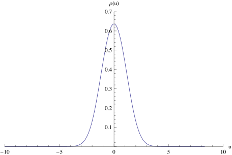
Figure 1: Ratio $\rho(u)$ for $\sigma=1$ over $-10\leq u\leq 10$, see (17).

Next we consider a practical application of the CRB for binary sensor networks.

IV Application: Biochemical source localisation

IV-A The measurement model and its derivatives

Localisation of a source of hazardous biochemical material, released in the atmosphere and transported by wind, is very important for public safety [8]. The measurement model $C_{i}(\mbox{\boldmath$\theta$})$ in this application is a suitable atmospheric dispersion model [9]. Such a model describes via mathematical equations the physical processes that govern the atmospheric dispersion of biological pathogens or chemical substances within the plume. We adopt in this study the Gaussian plume model, being the core of all regulatory atmospheric dispersion models [9].

Suppose a biochemical source is located at coordinates $(x_{0},y_{0},z_{0})$. The release rate of the source is $Q_{0}$. By convention, the wind direction coincides with the direction of the $x$ axis. The mean wind speed is denoted by $U$; the spread of the plume in $y$ and $z$ direction for $x>x_{0}$ is modelled by [10]

$$\sigma_{y} = \sigma_{v}(x-x_{0})/U$$ (18)

$$\sigma_{z} = \sigma_{w}(x-x_{0})/U,$$ (19)

respectively, where $\sigma_{v}$ and $\sigma_{w}$ are environmental parameters. In reality, $x_{0}$, $y_{0}$, $z_{0}$, $Q_{0}$, $U$, $\sigma_{v}$ and $\sigma_{w}$ are unknown parameters, although prior knowledge is available for some of them in the form of meteorological/environmental advice. For simplicity, however, we will focus on localisation only, that is, only the source coordinates $x_{0}$ and $y_{0}$ are assumed unknown, hence $\mbox{\boldmath$\theta$}=\left[x_{0}\;y_{0}\right]^{\intercal}$. The Gaussian plume model of a concentration measurement at $i$th sensor, $i=1,\dots,S$, located at coordinates $(x_{i}>x_{0},y_{i},z_{i}=0)$, is given by [10]

$$C_{i}(\mbox{\boldmath$\theta$})=\frac{Q_{0}}{\pi\sigma_{y_{i}}\sigma_{z_{i}}U}\exp\left\{-\frac{z_{0}^{2}}{2\sigma_{z_{i}}^{2}}\right\}\exp\left\{-\frac{(y_{i}-y_{0})^{2}}{2\sigma_{y_{i}}^{2}}\right\}.$$ (20)

Note that the plume spreads $\sigma_{y_{i}}$ and $\sigma_{z_{i}}$ in (20) are assigned the sensor index $i$, because they are computed at $x_{i}$.

In order to compute the information matrix (and the CRB), according to (15), we need to derive the partial derivatives $\partial C_{i}(\mbox{\boldmath$\theta$})/\partial x_{0}$ and $\partial C_{i}(\mbox{\boldmath$\theta$})/\partial y_{0}$. After few steps one can get [7]:

$$\frac{\partial C_{i}(\mbox{\boldmath$\theta$})}{\partial x_{0}}=\alpha+\beta+\gamma$$ (21)

with

$$\alpha =\frac{Q_{0}\sigma_{w}e^{-\frac{z_{0}^{2}}{2\sigma_{z_{i}}^{2}}}e^{-\frac{(y_{i}-y_{0})^{2}}{2\sigma_{y_{i}}^{2}}}}{\pi U^{2}\sigma_{y_{i}}\sigma_{z_{i}}^{2}},\hskip 2.84526pt\beta=\frac{Q_{0}\sigma_{v}e^{-\frac{z_{0}^{2}}{2\sigma_{z_{i}}^{2}}}e^{-\frac{(y_{i}-y_{0})^{2}}{2\sigma_{y_{i}}^{2}}}}{\pi U^{2}\sigma_{y_{i}}^{2}\sigma_{z_{i}}}$$

$$\gamma =\frac{Q_{0}e^{-\frac{z_{0}^{2}}{2\sigma_{z_{i}}^{2}}}e^{-\frac{(y_{i}-y_{0})^{2}}{2\sigma_{y_{i}}^{2}}}}{\pi U\sigma_{y_{i}}\sigma_{z_{i}}}\left[-\frac{(y_{i}-y_{0})^{2}\sigma_{v}}{U\sigma_{y_{i}}^{3}}-\frac{z_{0}^{2}\sigma_{w}}{U\sigma_{z_{i}}^{3}}\right]$$

Similarly,

$$\frac{\partial C_{i}(\mbox{\boldmath$\theta$})}{\partial y_{0}}=\frac{Q_{0}\,(y_{i}-y_{0})\,e^{-\frac{z_{0}^{2}}{2\sigma_{z_{i}}^{2}}}e^{-\frac{(y_{i}-y_{0})^{2}}{2\sigma_{y_{i}}^{2}}}}{\pi U\sigma_{y_{i}}^{3}\sigma_{z_{i}}}$$ (22)

IV-B Numerical analysis and verification

The CRB is computed and verified for a scenario plotted in Fig.2. The source is marked by the asterisk at coordinates $(10,15)$. The colours indicate the level of concentration of the released material on the ground, i.e. $z_{i}=0$. The area populated by binary sensors is indicated by a rectangle whose lower-left corner is at $(30,-40)$ m, and the upper right corner at $(240,50)$ m. The total number of binary sensors is $S=27$. The locations of sensors with measurements $b_{i}=1$ are marked by red squares, while those with $b_{i}=0$ are indicated by white circles, using threshold $\tau=0.0024$. Other parameters used in the simulation are as follows: $z_{0}=5$ m, $Q_{0}=5$ g/s, $U=3.5$ m/s, $\sigma_{v}=0.5$ m/s, $\sigma_{w}=0.2$ m/s. The standard deviation of noise $\sigma=0.0001$ g/m³. The covariance matrix of the prior pdf is $\mathbf{\Sigma}=\mbox{diag}[500^{2},\;500^{2}]$.

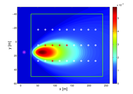
Figure 2: The scenario with $S=27$ sensors for numerical analysis and verification of the CRB.

The posterior CRB, $\mathbf{J}^{-1}$, in this case is a $2\times 2$ matrix, from which we can express the theoretically best achievable standard deviation of localisation error as

$$\sigma^{\mbox{\tiny crb}}_{loc}=\sqrt{\mbox{tr}\left[\mathbf{J}^{-1}\right]}.$$ (23)

This posterior standard deviation, as a function of the threshold $\tau$, is plotted by a solid green line in Fig.3 for the adopted scenario with binary sensors. The horizontal blue dashed line at $\sigma^{\mbox{\tiny crb}}_{loc}=\sqrt{\mbox{tr}\left[\mathbf{J^{p}}^{-1}\right]}=\sqrt{2\times 500^{2}}\approx 707$ m indicates the prior standard deviation of source location error; the horizontal red dotted line at $\sigma^{\mbox{\tiny crb}}_{loc}\approx 0.3$ m marks the value computed using the CRB for analog (non-quantised) measurements, via (16).

Note that, as discussed earlier, for too high and too low threshold values $\tau$, the posterior localisation uncertainty equals the prior uncertainty, because the information contained in the binary measurements equals zero (this is when all measurements are either zero or one). For a middle range of $\tau$ values, the posterior standard deviation of binary measurements approaches the posterior standard deviation of analog measurements (but never reaches it, as discussed earlier). This observation applies even when the number of sensors is increased, as demonstrated by the dash-dotted line in Fig.3: this line shows the posterior standard deviation of binary measurements $\sigma^{\mbox{\tiny crb}}_{loc}$ for $S=200\times 50=10,000$ sensors placed on a uniform grid inside the rectangular area indicated in Fig.2.

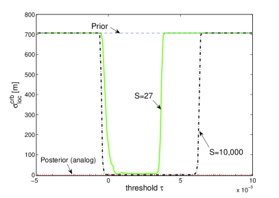
Figure 3: Standard deviation of localisation error using a binary sensor network, computed from the theoretical posterior CRB and plotted as a function of threshold $\tau$: the solid green line is for $S=27$ sensors; the dash-dotted line is for $S=10,000$ sensors

The theoretical bounds are next compared with the empirical estimation errors obtained using a Markov chain Monte Carlo (MCMC) based parameter estimation algorithm [11]. The MCMC algorithm is initialised by repeatedly drawing samples (candidate source coordinates) from the prior $\pi(\mbox{\boldmath$\theta$})$ until $n_{s}$ samples, whose likelihood (4) is greater than zero, are found. The sample with the highest value of the likelihood is selected as the starting point of the Metropolis-Hastings algorithm. The proposal distribution of the MCMC is Gaussian with the mean equal to the current sample and the covariance matrix equal to the theoretical CRB (details of the MCMC algorithms are omitted). The source location estimate is computed as the mean value of the last $n_{m}$ samples generated by the MCMC. Our practical implementation used the following values: $n_{s}=10$ and $n_{m}=10000$. Table I shows the results for the parameter values as listed above, using the threshold $\tau=0.0018$. Three different sensor placements are considered:
$\bullet$ Placement 1: $S=16$ sensors, with sensor $x$-coordinate $x_{i}\in\{40,100,160,220\}$m and $y$-coordinate $y_{i}\in\{-20,0,20,40\}$m; this placement is contained in placements 2 and 3.
$\bullet$ Placement 2: $S=28$ sensors, with $x_{i}\in\{40,$ $70,$ $100,$ $130,$ $160,$ $190,$ $220\}$m and $y_{i}\in\{-20,$ $40,$ $20,$ $40\}$m; this placement is contained in placement 3.
$\bullet$ Placement 3: $S=49$ sensors, with $x_{i}\in\{40,$ $70,$ $100,$ $130,$ $160,$ $190,$ $220\}$m and $y_{i}\in\{-20,-10,0,10,20,30,40\}$m.

Table I demonstrates a good agreement between the theoretical value $\sigma^{\mbox{\tiny crb}}_{loc}$ of (23) and the root-mean-squared (RMS) error $\widehat{\epsilon}_{loc}$ resulting from the MCMC localisation. The RMS error is computed as:

$$\widehat{\epsilon}_{loc}=\sqrt{\frac{1}{L}\sum_{\ell=1}^{L}\left[(\hat{x}^{\ell}_{0}-x_{0})^{2}+(\hat{y}^{\ell}_{0}-y_{0})^{2}\right]}$$ (24)

where $(\hat{x}^{\ell}_{0},\hat{y}^{\ell}_{0})$ are MCMC estimated coordinates of the source at the $\ell$th Monte Carlo run, with $\ell=1,\dots,L$ and $L=200$ is the total number of Monte Carlo runs.

TABLE I: Theoretical CRBs compared with the root mean square errors of an MCMC algorithm, averaged over 200 Monte Carlo runs

Sensor	Theoretical CRB	RMS error
placement	$\sigma^{\mbox{\tiny crb}}_{loc}$	$\widehat{\epsilon}_{loc}$
$(1)$	$5.75$ m	$7.33$ m
$(2)$	$3.93$ m	$4.08$ m
$(3)$	$0.68$ m	$2.55$ m

V Summary

The paper derived the theoretical Cramér-Rao lower bound for source estimation using measurements collected by a binary sensor network. The key result, given by (15), appears surprisingly simple and elegant. The bound is studied numerically in the context of a source of biochemical tracer (aerosol, gas) released in the atmosphere and transported by wind. Using a Gaussian plume dispersion model, the paper computed the theoretical bound and found that it approaches (but never reaches) the corresponding bound for analog (non-quantised) measurements, if the binary threshold is chosen properly. Finally, a good agreement between the theoretical bound and empirical errors (obtained using an MCMC based parameter estimation algorithm) is established.

References

- [1] J. Aslam, Z. Butler, F. Constantin, V. Crespi, G. Cybenko, and D. Rus, “Tracking a moving object with a binary sensor network,” in Proc. 1st Int. Conf. on Embedded Networked Sensor Systems, New York, NY, USA, 2003, SenSys ’03, pp. 150–161, ACM.
- [2] H. L. Van Trees, Detection, Estimation and Modulation Theory, John Wiley & Sons, 1968.
- [3] R. Niu and P. K. Varshney, “Target location estimation is sensor networks with quantized data,” IEEE Trans. Signal Processing, vol. 54, no. 12, pp. 4519–4528, 2006.
- [4] A. Ribeiro and G. B. Giannakis, “Bandwidth-constrained distributed estimation for wireless sensor networks - Part I: Gaussian case,” IEEE Trans. Signal Processing, vol. 54, no. 3, pp. 1131–1143, 2006.
- [5] P. Djuric, M. Vemula, and M. F. Bugallo, “Target tracking by particle filtering in binary sensor network,” IEEE Trans. Signal Processing, vol. 56, no. 6, pp. 2229–2238, 2008.
- [6] N. Patwari, J. N. Ash, S. Kyperountas, A. O. Hero III, R. L. Moses, and N. S. Correal, “Locating the nodes,” IEEE Signal Processing Magazine, pp. 54–68, 2005.
- [7] B. Ristic, A. Gunatilaka, and R. Gailis, “Achievable accuracy in parameter estimation of a Gaussian plume dispersion model,” in Proc. IEEE Workshop Statistical Signal Processing, Gold Coast, Australia, June/July 2014.
- [8] T. Zhao and A. Nehorai, “Detecting and estimating biochemical dispersion of a moving source in a semi-infinite medium,” IEEE Trans. Signal Processing, vol. 54, no. 6, pp. 2213–2225, 2006.
- [9] S. P. Arya, Pollution Meteorology and Dispersion, Oxford University Press, 1998.
- [10] A. Venkatram, V. Isakov, D. Pankratz, and J. Yuan, “Relating plume spread to meteorology in urban areas,” Atmospheric Environment, vol. 39, pp. 371–380, 2005.
- [11] C. P. Robert and G. Casella, Monte Carlo Statistical Methods, Springer, 2nd edition, 2004.