The Effect of Conjunctions on the Transit Timing Variations
of Exoplanets

Abstract

We develop an analytic model for transit timing variations produced by orbital conjunctions between gravitationally interacting planets. If the planetary orbits have tight orbital spacing, which is a common case among the Kepler planets, the effect of a single conjunction can be best described as: (1) a step-like change of the transit timing ephemeris with subsequent transits of the inner planet being delayed and those of the outer planet being sped up, and (2) a discrete change in sampling of the underlying oscillations from eccentricity-related interaction terms. In the limit of small orbital eccentricities, our analytic model gives explicit equations for these effects as a function of the mass and orbital separation of planets. We point out that a detection of the conjunction effect in real data is of crucial importance for the physical characterization of planetary systems from transit timing variations.

1 Introduction

Planetary orbits are less than ideal clocks. This is because various processes, including, for example, the gravitational interaction between planets, collaborate to produce fluctuations from perfect periodicity. The Transit Timing Variations (TTVs; Agol et al. 2005, Holman & Murray 2005), a method that has become increasingly important in the exoplanet research, exploits the effect of these fluctuations on the timing of planetary transits. It can be used to make useful inferences about the nature of planets in a system where at least one planet is transiting.

The TTVs caused by interacting planets come in several flavors. The long-periodic TTVs result from orbital variability on timescales much longer than the orbital period. Their detection therefore requires a long observation baseline (Heyl & Gladman 2007). The resonant and near-resonant TTVs occur when orbital periods, when divided by each other, are equal or nearly equal to a ratio of small integers. The planetary perturbations tend to build up in this situation, leading to TTVs with a large amplitude.

The detection of (near-)resonant TTVs is expected if a large set of transit observations is available, because some planetary systems are bound to have (near-)resonant orbits (either due to statistics or because they are driven to these orbits by formation processes). The description of planetary properties from (near-)resonant TTVs, however, is plagued with degeneracies, which may be resolved only under certain assumptions (Lithwick et al. 2012). This happens, in essence, because the (near-)resonant TTVs are limited in the information content.

This is where the short-periodic TTVs become useful. The short-periodic TTVs are produced by variations of orbits on a timescale comparable to the orbital period. In general, it can be shown that

$$-n_{i}\delta t_{i}=\delta\lambda_{i}-2\delta h_{i}+{3\over 2}(k_{i}\delta h_{i}+h_{i}\delta k_{i})+{\cal O}(e_{i}^{2})\ ,$$ (1)

where $\delta t_{i}$ is the short-periodic deviation of timing of planet $i$ from a linear ephemeris, $k_{i}=e_{i}\cos\varpi_{i}$, $h_{i}=e_{i}\sin\varpi_{i}$, and $n_{i}=2\pi/P_{i}$, where $P_{i}$ is the orbital period (Nesvorný 2009). Quantities $\delta\lambda_{i}$, $\delta h_{i}$ and $\delta k_{i}$ are the short-periodic variations of the mean longitude, $h_{i}$ and $k_{i}$, respectively.

The short-periodic variations $\delta\lambda_{i}$, $\delta h_{i}$ and $\delta k_{i}$ can be computed from perturbation theory. With $m_{i},a_{i},e_{i},i_{i},\varpi_{i},\Omega_{i},\lambda_{i}$ denoting the mass and orbital elements of planet $i$, we have

$$\delta\lambda_{i} = {1\over L_{i}}\left[2a_{i}{\partial\chi\over\partial a_{i}}+{\beta\over D_{i}}\left(x_{i}{\partial\chi\over\partial h_{i}}-y_{i}{\partial\chi\over\partial k_{i}}\right)\right]\ ,$$

$$\delta h_{i} = -{\beta\over L_{i}}\left[{\partial\chi\over\partial k_{i}}+{x_{i}\over D_{i}}{\partial\chi\over\partial\lambda_{i}}\right]\ ,$$

$$\delta k_{i} = {\beta\over L_{i}}\left[{\partial\chi\over\partial h_{i}}+{y_{i}\over D_{i}}{\partial\chi\over\partial\lambda_{i}}\right]\ ,$$ (2)

where $L_{i}=m_{i}\sqrt{GM_{*}a_{i}}$, $G$ is the gravitational constant, $M_{*}$ is the mass of the host star, $x_{i}=-\sqrt{2P_{i}}\sin\varpi_{i}$, $y_{i}=\sqrt{2P}_{i}\cos\varpi_{i}$, $P_{i}=L_{i}(1-\beta_{i})$, $D_{i}=\sqrt{2L_{i}(1+\beta_{i})}$ and $\beta_{i}=\sqrt{1-e_{i}^{2}}$. Function $\chi$ can be written as:

$$\chi = {Gm_{1}m_{2}\over a_{2}}\sum_{|k_{1}|+|k_{2}|\neq 0}\imath{C^{\mathbf{l},\mathbf{j}}_{\mathbf{k}}(\alpha)\over k_{1}n_{1}+k_{2}n_{2}}e_{1}^{l_{1}}e_{2}^{l_{2}}(\sin{i_{1}\over 2})^{j_{1}}(\sin{i_{2}\over 2})^{j_{2}}$$ (3)

$$\times \exp\imath(k_{3}\varpi_{1}+k_{4}\varpi_{2}+k_{5}\Omega_{1}+k_{6}\Omega_{2})\exp\imath(k_{1}\lambda_{1}+k_{2}\lambda_{2})$$

with $\imath=\sqrt{-1}$, $C^{\mathbf{l},\mathbf{j}}_{\mathbf{k}}(\alpha)=C^{\mathbf{l},\mathbf{j}}_{-\mathbf{k}}(\alpha)$, $\alpha=a_{1}/a_{2}<1$, and multi-indexes $\mathbf{l}=(l_{1},l_{2})$, $\mathbf{j}=(j_{1},j_{2})$ and $\mathbf{k}=(k_{1},k_{2},k_{3},k_{4},k_{5},k_{6})$. See Nesvorný & Morbidelli (2008) for the assumptions that led to the derivation of Eqs. (2) and (3). In brief, Eq. (2) does not include terms from the inclination of the transiting planet (assumed to be small), and Eq. (3) is given to the first-order in $m_{1}/M_{*}$ and $m_{2}/M_{*}$.

According to these equations, $\delta t_{i}$ contains Fourier terms with the $k_{1}\lambda_{1}+k_{2}\lambda_{2}$ harmonics. The amplitude of these terms is a complex function of $\alpha$, eccentricities and inclinations, but the ones with small $|k_{1}|$ and $|k_{2}|$ values are generally the most important (except if $k_{1}n_{1}+k_{2}n_{2}=0$ for arbitrary $k_{1}$ and $k_{2}$, indicating the presence of a resonance). It is also obvious, in the approximation of Eqs. (1)-(3), that $\delta t_{i}$ is proportional to $P_{i}$, independent of $m_{i}$, and scales linearly with the companion mass.

The short-periodic TTVs are more difficult to detect observationally then the (near-)resonant TTVs, because they generally have a small amplitude. If they are detected, however, they can be used to uniquely characterize the orbital properties of planets. This has been theoretically demonstrated in Nesvorný & Beaugé (2010) under the assumption that there is no a priori information about the (non-transiting) companion, and done in practice in Holman et al. (2010), and elsewhere. Intuitively, this can be understood because each Fourier term in Eq. (3) provides specific information about orbital elements. Thus, if at least a few of these terms are detected in real data, the information contained in the detection is high enough to make the inversion to orbital elements possible (e.g., Nesvorný et al. 2012).

An important component of the short-periodic TTVs, which is the main focus here, is produced by conjunctions between planets. The conjunction effect can be conveniently illustrated using Kepler-36c (Carter et al. 2012) and KOI-884.02 (Nesvorný et al. 2014) (see Figure 1). Kepler-36 is a doubly-transiting system, consisting of two planets on very tightly spaced orbits, with the two planets having significantly different masses (Carter et al. 2012). The KOI-884 system contains three known transiting planetary candidates, with the inner two displaying little or no sign of TTVs, while the outer one (KOI-884.02) exhibits significant TTVs. Nesvorný et al. (2014) used the TTVs of KOI-884.02 to detect an additional, unseen (i.e. non-transiting) planet just narrow of the outer 3:1 resonance with KOI-884.02 (orbital period ratio 2.93).

In the case of KOI-884.02, the effect of conjunctions is best seen for transit cycles 32 to 45 in Figure 1a, where three transits on a nearly linear ephemeris are offset from the next three transits. These discontinuities are produced at conjunctions with the outer massive planet ($M_{\rm p}\simeq 2.4\ M_{\rm J}$, where $M_{\rm J}$ is the mass of Jupiter; Nesvorný et al. 2014). The TTVs of Kepler-36c, on the other hand, are a series of approximately linear segments that are tilted relative to each other at different angles (Carter et al. 2012). These discontinuities correspond to the orbital conjunctions between Kepler-36c and the inner transiting planet Kepler-36b. In this case, the very tight spacing of two orbits at (or very near to) the 7:6 resonance implies the physical distance between planets to be small near conjunctions, and large variations are therefore expected. In general, for a $(j+1)$:$j$ resonance, we expect the conjunctions to occur in every $j$ periods of the outer planet (and $j+1$ periods of the inner one). This is why, in Figure 1b, groups of $j=6$ transits share the same linear ephemeris (note that some transits are missing due to instrumental and other issues).

It is not straightforward to theoretically understand the effect of conjunctions from Eqs. (1)-(3), mainly because the TTV discontinuities occurring at conjunctions are difficult to approximate by the Fourier series, and because these equations include many different terms such that it is not clear which ones are responsible for the conjunction effect. The goal of this paper is to present a simple model for the conjunction effect that can be used as an intuitive guideline for more realistic modeling of cases such as the ones shown in Figure 1.

In Section 2, we derive an analytic model of conjunctions in the limit of small orbital eccentricities. In Section 3, we test our model by comparing it with numerical integrations of the full equations of motion, and determine the domain of parameters where the analytic model is valid. In Section 4, we show how the magnitude of the conjunction effect scales with different parameters. Finally, in Section 5, we discuss how the detection of the conjunction effect can be used to confirm and characterize transiting planetary systems.

2 Analytic Model

2.1 Equations of Motion

We consider a system of two planets with masses $m_{1}$ and $m_{2}$ orbiting about a central star with mass $M_{*}$. The planetary orbits are assumed to be nearly coplanar and nearly circular, with planet 1 on the interior and planet 2 on the exterior. The analytic model is developed in variables $a_{i}$, $\lambda_{i}$, and $z_{i}=e_{i}\exp(\imath\varpi_{i})$, where index $i=1,2$ stands for the two planets. These variables are non-singular for $e_{i}\rightarrow 0$, and non-canonical, with the later being appropriate because we do not aim at developing the theory beyond the lowest order in eccentricity and beyond the linear terms in $m_{1}/M_{*}$ and $m_{2}/M_{*}$. The inclination terms are ignored because they appear in the second and higher powers, and are therefore not overly important for the TTVs (as we show in Section 4). With that being clarified, the Lagrange equations describing the evolution of orbital elements are

$$\frac{da_{i}}{dt} = -\frac{2}{\mu_{i}n_{i}a_{i}}\frac{\partial{\cal H}_{\rm per}}{\partial\lambda_{i}}\;,$$ (4)

$$\frac{d\lambda_{i}}{dt} = n_{i}+\frac{2}{\mu_{i}n_{i}a_{i}}\frac{\partial{\cal H}_{\rm per}}{\partial a_{i}}+{\cal O}(e)\;,$$ (5)

$$\frac{dz_{i}}{dt} = -\frac{2\,\imath}{\mu_{i}n_{i}a_{i}^{2}}\frac{\partial{\cal H}_{\rm per}}{\partial z_{i}}+{\cal O}(e)\;,$$ (6)

where $\mu_{i}$ is the reduced mass and $n_{i}$ is the mean motion. All terms that are explicitly the first or higher eccentricity powers were removed from Eqs. (5) and (6). ${\cal H}_{\rm per}$ denotes the perturbation part of the Hamiltonian.

We follow Malhotra (1993) and split the Hamiltonian, ${\cal H}={\cal H}_{\rm Kep}+{\cal H}_{\rm per}$, such that

$${\cal H}_{\rm Kep}=-G\,\frac{\mu_{1}M_{1}}{2a_{1}}-G\,\frac{\mu_{2}M_{2}}{2a_{2}}\;,$$ (7)

where $M_{1}=M_{*}+m_{1}$, $\mu_{1}=M_{*}m_{1}/M_{1}$, $M_{2}=M_{*}(M_{1}+m_{2})/M_{1}$, and $\mu_{2}=M_{1}m_{2}/(M_{1}+m_{2})$. This choice implies that the unperturbed motion satisfies $n_{1}^{2}a_{1}^{3}=GM_{1}$ and $n_{2}^{2}a_{2}^{3}=GM_{2}$. At the unperturbed level, $a_{1}$, $a_{2}$, $z_{1}$ and $z_{2}$ are constant, and $\lambda_{1}=n_{1}t+\lambda_{1}^{(0)}$ and $\lambda_{2}=n_{2}t+\lambda_{2}^{(0)}$, where $\lambda_{1}^{(0)}$ and $\lambda_{2}^{(0)}$ are the initial phases at $t=0$.

As for the interaction term, up to the first power in $m_{1}/M_{*}$, $m_{2}/M_{*}$ and eccentricities, we have ${\cal H}_{\rm per}={\cal H}_{0}+{\cal H}_{1}$, where the part independent of eccentricities is

$${\cal H}_{0}=G\,\frac{m_{1}m_{2}}{a_{2}}\left[\alpha\cos\psi-P(\alpha,\psi)\right]\;$$ (8)

with $\alpha=a_{1}/a_{2}$, synodic angle $\psi=\lambda_{1}-\lambda_{2}$, and

$$P(\alpha,\psi)=\left(1-2\alpha\cos\psi+\alpha^{2}\right)^{-1/2}\;.$$ (9)

The first-order eccentricity term, ${\cal H}_{1}$, is somewhat more complicated:

$${\cal H}_{1}=G\,\frac{m_{1}m_{2}}{a_{2}} \times \Re\biggl{(}c_{0}^{+}\,z_{1}\,e^{-\imath\lambda_{1}}-d_{0}^{+}\,z_{2}\,e^{-\imath\lambda_{2}}$$

$$+ \sum_{j\geq 1}\left[\left(c_{j}^{-}+\alpha\delta_{j1}\right)z_{1}\,e^{-\imath(j\psi+\lambda_{1})}+\left(c_{j}^{+}-3\alpha\delta_{j1}\right)z_{1}\,e^{\imath(j\psi-\lambda_{1})}\right]$$

$$- \sum_{j\geq 1}\left[d_{j}^{-}\,z_{2}\,e^{-\imath(j\psi+\lambda_{2})}+\left(d_{j}^{+}-4\alpha\delta_{j1}\right)z_{2}\,e^{\imath(j\psi-\lambda_{2})}\right]\biggr{)}\;$$

(Malhotra 1993, Agol et al. 2005). Here, $\Re$ denotes the real part, $\delta_{j1}$ is the Kronecker delta, $c_{j}^{\pm}=\partial_{\alpha}b^{(j)}_{1/2}\pm 2jb^{(j)}_{1/2}$, $d_{j}^{\pm}=c_{j}^{\pm}+b^{(j)}_{1/2}$, and $\partial_{\alpha}b^{(j)}_{1/2}=\alpha\,(\partial/\partial\alpha)b^{(j)}_{1/2}$ for $j\geq 0$. Symbols $b^{(j)}_{1/2}(\alpha)$ denote the Laplace coefficients. They are best evaluated from $b^{(0)}_{1/2}=(2/\pi)\,{\bf K}(\alpha)$ and $b^{(1)}_{1/2}=2\,[{\bf K}(\alpha)-{\bf E}(\alpha)]/(\pi\alpha)$, where ${\bf K}$ and ${\bf E}$ are the complete elliptic integrals of the first and second kinds, respectively, and the efficient and stable recurrences recommended in Brouwer & Clemence (1961). The derivatives $\partial_{\alpha}b^{(j)}_{1/2}(\alpha)$ were also obtained from the recurrences defined in Brouwer & Clemence (1961).

2.2 The First-Order Solution

The first-order perturbation solution can be obtained by inserting the unperturbed motion (i.e., corresponding to ${\cal H}_{\rm Kep}$) into the right-hand sides of the Eqs. (4)-(6), and performing a quadrature. Below we compute this quadrature in the time interval from $\psi=-\pi$ to $\psi=\pi$, i.e. over one conjunction cycle. For the reasons explained in the next paragraph we find it useful to formulate the results of the quadrature in terms of the synodic angle $\psi$, rather than of time, but these two formulations are interchangeable because $\psi=(n_{1}-n_{2})t-\pi$ (with $\lambda_{2}^{(0)}-\lambda_{1}^{(0)}=\pi$). To keep things simple, we perform our calculation only to the lowest order in eccentricities, where the resulting expressions become independent of $e_{1}$ and $e_{2}$.

If $\alpha$ is somewhat large (but not too large to lead to the co-orbital motion), the orbital spacing is relatively tight (as in many Kepler systems), and the interaction between planets happens almost exclusively at conjunctions. This is the case when using $\psi$ and the interaction Hamiltonian in Eqs. (8)-(2.1) is the most helpful, because the ‘impulsive’ effects of conjunctions are well captured by a nearly discrete change when $\psi\simeq 0$. If, instead, $\alpha$ is small ($\alpha<0.5$), the conjunction effects cannot be easily isolated, and the Fourier series in Eq. (3) becomes more a appropriate representation of the TTVs.

2.2.1 Semimajor Axis and Mean Longitude

We first discuss the variations of semimajor axis and mean longitude described by Eqs. (4) and (5). In this case, we use ${\cal H}_{\rm per}={\cal H}_{0}$ in the right-hand side of Eq. (4), and perform the quadrature to obtain

$$\delta a_{1} = -2\,\nu_{1}a_{1}\,\frac{m_{2}}{M_{*}}\,Q\left(\alpha,\psi\right)\;,$$ (11)

$$\delta a_{2} = 2\,\nu_{2}a_{2}\,\frac{m_{1}}{M_{*}}\,Q\left(\alpha,\psi\right)\;,$$ (12)

where $\delta a_{1}$ and $\delta a_{2}$ denote the semimajor-axis variations of the inner and outer planets, $\nu_{1}=n_{1}/(n_{1}-n_{2})$ and $\nu_{2}=n_{2}/(n_{1}-n_{2})$. Assuming that $\delta a_{1}=\delta a_{2}=0$ at $\psi=-\pi$ (i.e., $\pi$ away from the conjunction), the function $Q$ can be written as

$$Q\left(\alpha,\psi\right)=\alpha\cos\psi-P\left(\alpha,\psi\right)+1+\frac{\alpha^{2}}{1+\alpha}\;.$$ (13)

Here and in the following, $\psi$ has to be understood as an unperturbed angle that linearly increases with time ($\psi=(n_{1}-n_{2})t-\pi$, where $n_{1}$ and $n_{2}$ are the unperturbed orbital frequencies defined by ${\cal H}_{\rm Kep}$). Note that Eqs. (11) and (12) obey the law of the total angular momentum conservation, because $m_{1}\,\delta a_{1}/(n_{1}a_{1})+m_{2}\,\delta a_{2}/(n_{2}a_{2})=0$.

A change of the semimajor axis leads to a change of the mean motion according to

$$\delta n_{1}=-\frac{3}{2}\frac{n_{1}}{a_{1}}\,\delta a_{1}\;\ ,$$ (14)

and similarly for the outer orbit. This term, together with the derivative in the second term in Eq. (5) (where again ${\cal H}_{\rm per}={\cal H}_{0}$), allow us to calculate the variation of the mean longitude. The quadrature gives

$$\delta\lambda_{1}=\frac{m_{2}}{M_{*}}\,\Bigl{[}A_{1}(\alpha)+A_{2}(\alpha)\,\psi+A_{3}(\alpha)\,\sin\psi+A_{4}\left(\psi,\alpha\right)\Bigr{]}\;$$ (15)

with

$$A_{1}(\alpha) \!\!\!=\!\!\! 3\pi\,\alpha\nu_{1}^{2}\left[1+\frac{\alpha^{2}}{1+\alpha}\right]+2\,\alpha\nu_{1}\left[\left(2-3\nu_{1}\right){\bf K}(\alpha)-\frac{2\,{\bf E}(\alpha)}{1-\alpha^{2}}\right]\;,$$

$$A_{2}(\alpha) \!\!\!=\!\!\! 3\,\alpha\nu_{1}^{2}\left[1+\frac{\alpha^{2}}{1+\alpha}\right]\;,$$ (16)

$$A_{3}(\alpha) \!\!\!=\!\!\! \alpha^{2}\nu_{1}\left(2+3\nu_{1}\right)\;,$$ (17)

$$A_{4}(\psi,\alpha) \!\!\!=\!\!\! 2\,\alpha\nu_{1}\left[\left(1-3\nu_{1}\right)\frac{F(\delta,r)}{1+\alpha}-\frac{E(\delta,r)}{1-\alpha}\right]\;,$$ (18)

where $F(\delta,r)$ and $E(\delta,r)$ are incomplete elliptic integrals of the first and second kind with modulus $r=2\sqrt{\alpha}/(1+\alpha)$ and amplitude $\sin\delta=(1+\alpha)\,P(\alpha,\psi)\,\sin\psi/2$.

Similarly, the mean longitude variation of the outer planet is found to be

$$\delta\lambda_{2}=\frac{m_{1}}{M_{*}}\,\Bigl{[}B_{1}(\alpha)+B_{2}(\alpha)\,\psi+B_{3}(\alpha)\,\sin\psi+B_{4}\left(\psi,\alpha\right)\Bigr{]}\;$$ (19)

with

$$B_{1}(\alpha) \!\!\!=\!\!\! -3\pi\,\nu_{2}^{2}\left[1+\frac{\alpha^{2}}{1+\alpha}\right]+2\,\nu_{2}\left[3\nu_{2}\,{\bf K}(\alpha)+\frac{2\,{\bf E}(\alpha)}{1-\alpha^{2}}\right]\;,$$

$$B_{2}(\alpha) \!\!\!=\!\!\! -3\,\nu_{2}^{2}\left[1+\frac{\alpha^{2}}{1+\alpha}\right]\;,$$ (20)

$$B_{3}(\alpha) \!\!\!=\!\!\! -\alpha\nu_{2}\left(4+3\nu_{2}\right)\;,$$ (21)

$$B_{4}(\psi,\alpha) \!\!\!=\!\!\! 2\,\nu_{2}\left[\left(1+3\nu_{2}\right)\frac{F(\delta,r)}{1+\alpha}+\frac{E(\delta,r)}{1-\alpha}\right]\;.$$ (22)

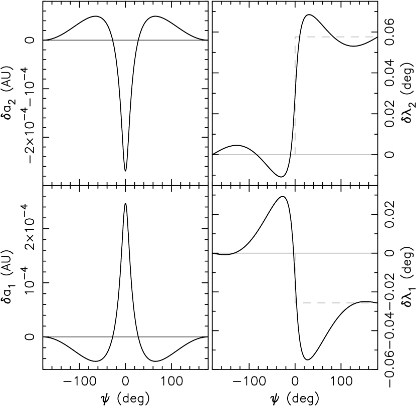
Figure 2: The effect of a single conjunction on $\delta a_{1}$ and $\delta a_{2}$ (left; computed from Eqs. (11) and (12)), and $\delta\lambda_{1}$ and $\delta\lambda_{2}$ (right; computed from Eqs. (15) and (19)). Here, the two planets have masses $m_{1}=m_{2}=10^{-5}\ M_{*}$, with $M_{*}=M_{\odot}$, and semimajor axes $a_{1}=0.84$ AU and $a_{2}=1$ AU. The evolution is shown as a function of the synodic angle $\psi=\lambda_{1}-\lambda_{2}$, where $\lambda_{1}$ and $\lambda_{2}$ are unperturbed mean longitudes of the two planets. The conjunction occurs when $\psi\simeq 0$. Notably, the semimajor axis of the inner (outer) planet increases (decreases) during the conjunction, while the mean longitudes of the two planets suffer a step-like discontinuity.

The expressions in Eqs. (15) and (19) have the same structure revealing the underlying effects of planetary conjunctions. The first term in the right-hand sides of these equations, independent of $\psi$, reflects a nearly step-like discontinuity of the mean longitude near the conjunction. The amplitude of this discontinuity is equal to $2A_{1}m_{2}/M_{*}$ for the inner planet, and $2B_{1}m_{1}/M_{*}$ for the outer planet. Figure 2 shows an example for $a_{1}=0.84$ AU, $a_{2}=1$ AU, $m_{1}/M_{*}=m_{2}/M_{*}=10^{-5}$, and $M_{*}=M_{\odot}$, where $M_{\odot}$ is the solar mass.

2.2.2 Eccentricity and Apsidal Longitude

Equation (1) shows that the TTVs depend not only on the variation of the mean longitude, but also on variation of eccentricity and apsidal longitude. To the lowest order in eccentricity, $\delta t_{i}$ becomes

$$-n_{i}\,\delta t_{i}=\delta\lambda_{i}+\delta\lambda_{i}^{\rm eff}+{\cal O}(e)\;,$$ (23)

where $\delta\lambda_{i}$ was computed in Section 2.2.1, and $\delta\lambda_{i}^{\rm eff}$ is the effective contribution from the short-periodic variations of $e_{i}$ and $\varpi_{i}$ (e.g., Nesvorný & Morbidelli 2008). Using the complex variable $z_{i}$ defined in Section 2.1. we have

$$\delta\lambda_{i}^{\rm eff}=\imath\left(\delta z_{i}\,e^{-\imath\lambda_{i}}-\delta z_{i}^{*}\,e^{\imath\lambda_{i}}\right)\;,$$ (24)

where $\delta z_{i}$ is the variation of $z_{i}$, $\delta z_{i}^{*}$ is the complex conjugate, and $\lambda_{i}$ is the unperturbed mean longitude. If the actual transits occur when $\lambda_{i}\simeq 0$, the above expression reduces, consistently with Eq. (1), to $\delta\lambda_{i}^{\rm eff}=-2\delta h_{i}+{\cal O}(e_{i})$.

The first-order approximation of $\delta z_{i}$ is obtained by inserting unperturbed motion into the right-hand side of Eq. (6) and performing the quadrature. We find that

$$\delta\lambda_{1}^{\rm eff}=\frac{m_{2}}{M_{*}}\Bigl{[}C_{1}(\alpha)\sin\left[\nu_{1}\left(\psi+\pi\right)\right]+\sum_{j\geq 1}D_{1}^{j}(\alpha)\sin j\psi\Bigr{]}\;,$$

where

$$C_{1}(\alpha) \!\!\!=\!\!\! \alpha\biggl{[}\partial_{\alpha}b_{1/2}^{(0)}+2\,\alpha\,\frac{\nu_{1}\left(3\nu_{1}-2\nu_{2}\right)}{\nu_{2}\left(2\nu_{1}-\nu_{2}\right)}-2\,\nu_{1}\sum_{j\geq 1}\left(-1\right)^{j}\frac{\nu_{1}\,\partial_{\alpha}b_{1/2}^{(j)}+2j^{2}\,b_{1/2}^{(j)}}{j^{2}-\nu_{1}^{2}}\biggr{]}\;,$$ (25)

$$D_{1}^{j}(\alpha) \!\!\!=\!\!\! 2\,\delta_{j1}\,\alpha^{2}\frac{\nu_{1}\left(3\nu_{1}-2\nu_{2}\right)}{\nu_{2}\left(2\nu_{1}-\nu_{2}\right)}+2j\,\alpha\nu_{1}\frac{\partial_{\alpha}b_{1/2}^{(j)}+2\nu_{1}\,b_{1/2}^{(j)}}{j^{2}-\nu_{1}^{2}}\;.$$ (26)

Similarly, for the outer planet we obtain

$$\delta\lambda_{2}^{\rm eff}=\frac{m_{1}}{M_{*}}\Bigl{[}C_{2}(\alpha)\sin\left[\nu_{2}\left(\psi+\pi\right)\right]+\sum_{j\geq 1}D_{2}^{j}(\alpha)\sin j\psi\Bigr{]}\;,$$ (27)

where

$$\!\!\!\!\!\!C_{2}(\alpha) \!\!\!=\!\!\! 4\,\alpha\,\frac{\nu_{2}}{\left(\nu_{1}-2\nu_{2}\right)}-\left(\partial_{\alpha}b_{1/2}^{(0)}+b_{1/2}^{(0)}\right)+2\,\nu_{2}\sum_{j\geq 1}\left(-1\right)^{j}\frac{\nu_{2}\,\partial_{\alpha}b_{1/2}^{(j)}+\left(2j^{2}+\nu_{2}\right)b_{1/2}^{(j)}}{j^{2}-\nu_{2}^{2}}\biggr{]}\;,$$ (28)

$$\!\!\!\!\!\!D_{2}^{j}(\alpha) \!\!\!=\!\!\! 4\,\delta_{j1}\,\alpha\frac{\nu_{2}}{\nu_{1}-2\nu_{2}}-2j\,\nu_{2}\frac{\partial_{\alpha}b_{1/2}^{(j)}+\left(2\nu_{2}+1\right)\,b_{1/2}^{(j)}}{j^{2}-\nu_{2}^{2}}\;.$$ (29)

The coefficients $C_{1}(\alpha)$, $C_{2}(\alpha)$, $D_{1}^{j}(\alpha)$ and $D_{2}^{j}(\alpha)$ defined above have singularities at the first-order mean motion resonances, which is a consequence of the perturbation method applied here. For example, when $n_{1}/n_{2}=j/(j-1)$, we have $\nu_{1}=j$, which causes a zero divisor in Eqs. (25) and (26). Similarly, when $n_{1}/n_{2}=(j+1)/j$ we have $\nu_{2}=j$, implying zero divisors in Eqs. (28) and (29). Interestingly, however, when these expressions combine in Eqs. (2.2.2) and (27) into variables important for the TTVs, the singularities disappear such that both $\delta\lambda_{1}^{\rm eff}$ and $\delta\lambda_{2}^{\rm eff}$ are well defined at resonances. This can be most easily verified by assuming that $n_{1}/n_{2}=j/(j-1)+\varepsilon$ or $n_{1}/n_{2}=(j+1)/j+\varepsilon$, where $\varepsilon$ is a small quantity, and showing that $\lambda_{1}^{\rm eff}$ and $\lambda_{2}^{\rm eff}$ are non-divergent when $\varepsilon\rightarrow 0$.

To derive the expressions in Eqs. (2.2.2) and (27) we assumed that $e_{1}=0$ and $e_{2}=0$ when $\psi=-\pi$. Note that, in this case, $\delta\lambda_{i}^{\rm eff}$ is independent of the initial phases $\lambda_{1}^{(0)}$ and $\lambda_{2}^{(0)}$. Together with a similar result obtained in Section 2.2.1, this implies that $\delta t_{i}$ will also be independent of $\lambda_{i}^{(0)}$ (see Section 2.3). It will only depend on the orbital period, $m_{1}/M_{*}$, $m_{2}/M_{*}$ and $\alpha$.

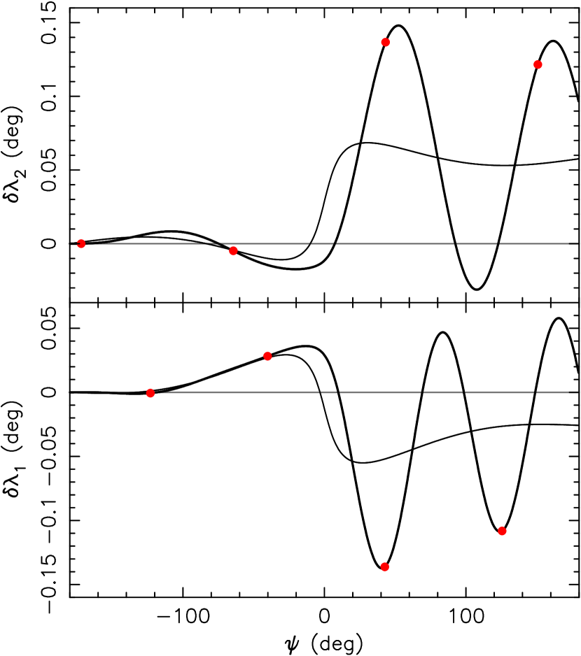
Figure 3: The effect of a single conjunction on $\delta\lambda_{1}$ (bottom panel) and $\delta\lambda_{2}$ (top panel) for two planets with masses $m_{1}=m_{2}=10^{-5}\ M_{*}$ ($M_{*}=M_{\odot}$), semimajor axes $a_{1}=0.84$ AU and $a_{2}=1$ AU, and initially circular orbits. The conjunction between the two planets occurs when $\psi=\lambda_{1}-\lambda_{2}\simeq 0$. The thin lines show the direct variation of $\delta\lambda_{i}$ from Eqs. (15) and (19). The bold lines show the combined effect, $\delta\lambda_{i}+\delta\lambda_{i}^{\rm eff}$, where $\delta\lambda_{i}^{\rm eff}$ stands for the effective contribution of eccentricities and apsidal longitudes. Assuming that both planets are transiting the red symbols show the expected transit cadence.

Figure 3 illustrates the role of $\delta\lambda_{i}^{\rm eff}$ in an example with $a_{1}=0.84$ AU, $a_{2}=1$ AU, $m_{i}=10^{-5}\ M_{*}$, $M_{*}=M_{\odot}$, and zero initial eccentricities. The effects of $\delta\lambda_{i}^{\rm eff}$ are initially small, but when small orbital eccentricities are excited during the conjunction (i.e., when $\psi\simeq 0$), $\delta t_{i}$ becomes a composite of two terms with comparable magnitudes: (i) a step-like change produced by the direct variation $\delta\lambda_{i}$ (Section 2.2.1), and (ii) oscillations from $\delta\lambda_{i}^{\rm eff}$. According to Eqs. (2.2.2) and (27), the oscillatory part has a rich spectrum of Fourier terms with frequencies $n_{1}$, $n_{2}$ and $j(n_{1}-n_{2})$.

A general solution corresponding to small values of the initial eccentricities $e_{1}^{(0)}$ and $e_{2}^{(0)}$, can be obtained by adding $2\,e_{1}^{(0)}\sin\left[\nu_{1}\left(\psi+\phi_{1}^{(0)}\right)\right]$ to Eq. (2.2.2) and $2\,e_{2}^{(0)}\sin\left[\nu_{2}\left(\psi+\phi^{(0)}_{2}\right)\right]$ to Eq. (27). Here, $\phi_{i}^{(0)}=(\lambda_{i}^{(0)}-\varpi_{i}^{(0)})/\nu_{i}+\pi$, where $\varpi_{i}^{(0)}$ are the apsidal longitudes of the two orbits when $\psi=-\pi$. Since, by definition, $\lambda_{2}^{(0)}=\lambda_{1}^{(0)}+\pi$, the general solution adds $e_{i}^{(0)}$, $\varpi_{i}^{(0)}$ and $\lambda_{1}^{(0)}$ (or $\lambda_{2}^{(0)}$) to the list of parameters.

2.3 Transit Timing Variations

The equations derived above can be used to compute $\delta\lambda_{i}+\delta\lambda_{i}^{\rm eff}$ as a function of the synodic angle $\psi$ in the interval $-\pi\leq\psi<\pi$. To be able to track changes over the successive rotations of $\psi$, we need to add a constant term to $\delta\lambda_{i}$ that expresses how $\delta\lambda_{i}$ changed during the previous conjunction. For an arbitrary $\psi\geq-\pi$, and denoting ${\rm{\bf int}}[x]$ the integer part of $x$, this term is

$$\delta\lambda_{1}^{\rm add}=2\,\frac{m_{2}}{M_{*}}\,A_{1}(\alpha)\,{\rm{\bf int}}\left[(\psi+\pi)/2\pi\right]\;$$ (30)

for the inner planet, and

$$\delta\lambda_{2}^{\rm add}=2\,\frac{m_{1}}{M_{*}}\,B_{1}(\alpha)\,{\rm{\bf int}}\left[(\psi+\pi)/2\pi\right]\;$$ (31)

for the outer planet. Adding this term successively each time $\psi$ increases by $2\pi$ leads to a situation where $\delta t_{i}$ either decreases (for the inner planet) or increases (for the outer one) in a series of steps. Equations (2.2.2)-(29) express the general dependence of $\delta\lambda_{i}^{\rm eff}$ on $\psi$ in that they can be used to compute the conjunction effect over the successive rotations of $\psi$. To do so, $\psi=(n_{1}-n_{2})t-\pi$ needs to be substituted into Eqs. (2.2.2) and (27). With these provisions, $\delta t_{i}$ can be computed for any $t\geq 0$.

Here we are mainly interested in the transit timing. We therefore assume that the observer detects transits on a (nearly) linear ephemeris, $t_{i}^{k}=kP_{i}+t_{i}^{0}$, where $t_{i}^{0}>0$ is the epoch of the first transit, $k\geq 1$ denotes the subsequent transit cycles, and $t_{i}^{k}$ are the subsequent transit epochs. This gives $\psi_{i}^{k}=2\pi k/\nu_{i}+(n_{1}-n_{2})t_{i}^{0}-\pi$, where $\psi_{i}^{k}$ denotes the value of the synodic angle corresponding to the $k+1$ transit of planet $i$. Substituting this into Eqs. (2.2.2) and (27), and dropping all constant terms (i.e., those independent of $k$), we find that:

$$\delta t_{1}^{k}=-{P_{1}\over 2\pi}{m_{2}\over M_{*}}\left[A(\psi_{1}^{k})+2A_{1}{\rm{\bf int}}\left[{k\over\nu_{1}}+{t_{1}^{0}\over P_{\psi}}\right]+\sum_{j\geq 1}(-1)^{j}D_{1}^{j}\sin\left(2\pi j\left[{k\over\nu_{1}}+{t_{1}^{0}\over P_{\psi}}\right]\right)\right]$$ (32)

and

$$\delta t_{2}^{k}=-{P_{2}\over 2\pi}{m_{1}\over M_{*}}\left[B(\psi_{2}^{k})+2B_{1}{\rm{\bf int}}\left[{k\over\nu_{2}}+{t_{2}^{0}\over P_{\psi}}\right]+\sum_{j\geq 1}(-1)^{j}D_{2}^{j}\sin\left(2\pi j\left[{k\over\nu_{2}}+{t_{2}^{0}\over P_{\psi}}\right]\right)\right]$$ (33)

Here we denoted $A(\psi_{1}^{k})=A_{2}\psi_{1}^{k}+A_{3}\sin\psi_{1}^{k}+A_{4}(\psi_{1}^{k})$, $B(\psi_{2}^{k})=B_{2}\psi_{2}^{k}+B_{3}\sin\psi_{2}^{k}+B_{4}(\psi_{2}^{k})$, and synodic period $P_{\psi}=2\pi/(n_{1}-n_{2})$. Note that $A$, $B$, $A_{1}$, $B_{1}$ $D_{1}^{j}$ and $D_{2}^{j}$ are explicit functions of $\alpha$ as defined in Sections 2.2.1 and 2.2.2. Also note that Eqs. (32) and (33) are related to Eqs. (A7) and (A8) previously derived in the appendix of Agol et al. (2005).

Equations (32) and (33) describe the effect of conjunctions on the TTVs. The three terms present in these equations stand for: the (i) modulation of $\delta t_{i}$ from $\delta\lambda_{i}$ during a single rotation of the synodic angle, (ii) total change of $\delta t_{i}$ from $\delta\lambda_{i}$ over all previous synodic cycles, and (iii) periodic terms from the eccentricity-related perturbations. The expressions for (iii) are non-divergent, because if $\nu_{1}=j$ (or $\nu_{2}=j$) the variable part of the corresponding sinusoidal terms vanishes from Eq. (32) (or Eq. (33)).

Notably, the sinusoidal terms in Eqs. (32) and (33) originate from terms with $\sin j\psi$ (see Eqs. (2.2.2) and (27)) and are $2\pi$-periodic in $\psi$. Therefore, as far as these periodic terms are concerned, there is no difference between the first, second, or any other cycle of $\psi$. The difference between the TTVs in different cycles of $\psi$ arises, instead, by how fixed periodic terms are sampled by TTV observations. For given $\alpha$, it turns out that the periodic term with the largest amplitude $D_{1}^{j}(\alpha)$ (or $D_{2}^{j}(\alpha)$) is the one with $j\sim\nu_{1}$ in Eq. (32) (or $j\sim\nu_{2}$ in Eq. (33)). As shown in Eq. (32) (or Eq. (33), however, these terms will be sampled with $\sim 2\pi k$ cadence and will therefore have only a limited impact on the TTVs.

3 Validity Domain of the Analytic Model

The analytic model developed in the previous sections can be used as a guideline to understand the basic effects of conjunctions on the TTVs. We will discuss these effects, and their scaling with different parameters, in Section 4. Before we do so, however, we first establish the domain of validity of the analytic model by comparing the results to those obtained from an exact $N$-body integration. This comparison was done with the $N$-body code described in Nesvorný et al. (2013), where the TTVs are computed with an efficient and precise algorithm (also see Deck et al. 2014).

Figure 4 illustrates the results for the test case previously shown in Figures 2 and 3. Here the results of the analytic model are in an excellent agreement with those obtained from the $N$-body integration. This was expected because the parameters of the test case were set to be in the domain where the analytic model should be valid (e.g., small planetary masses, $\alpha$ not too large, and $e_{i}^{(0)}=0$).

In general, however, the analytic model is obviously only an approximation of the conjunction effect. First, the two orbits were assumed to be strictly coplanar. Second, we assumed that $m_{i}\ll M_{*}$, such that ${\cal H}_{\rm per}$ can be treated as a perturbation of ${\cal H}_{\rm Kep}$. Terms of the second and higher orders in $m_{i}/M_{*}$ were not included. Third, we assumed that $e_{i}\ll 1$, expanded the Hamiltonian in powers of $e_{i}$, and retained only the lowest power of $e_{i}$. We therefore expect the analytic model to be valid only for very nearly circular orbits of both planets.

Figure 5 illustrates the approximate nature of the analytic model. To make this figure, we surveyed a range of orbital separations and eccentricities ($0.5<\alpha<0.9$, $0<e_{1}^{(0)}<0.1$ and $0<e_{2}^{(0)}<0.1$). Other parameters were held fixed ($m_{i}=10^{-5}\,M_{*}$, $M_{*}=M_{\odot}$). In each case, we followed dynamics over one conjunction cycle and determined the (i) amplitude of $\delta t_{i}$ variation produced as a result of conjunction, and (ii) the difference between analytically and numerically computed $\delta t_{i}$ when $\psi$ approaches $\pi$ (i.e., at the end of the conjunction cycle). From this, by dividing (ii) by (i), we computed the relative error of the analytic model as a function of $\alpha$, $e_{1}^{(0)}$ and $e_{2}^{(0)}$.

From Figure 5 we see that the analytic model is valid only for small eccentricities, and the eccentricity threshold ($e_{\rm crit}$) beyond which the relative error is excessive (say $>$10%) is a strong function of the radial separation between orbits. For example, $e_{\rm crit}\simeq 0.1$ for $\alpha=0.5$ while $e_{\rm crit}\simeq 0.01$ for $\alpha=0.8$, This is expected because the second and higher order effects in $m_{i}/M_{*}$, neglected in our analytic model, should become important with increasing $\alpha$. Also, we would need to include eccentricity terms beyond the lowest power to make the analytic model more generally valid for larger eccentricities.

We used $m_{i}/M_{*}=10^{-5}$ in Figure 5, but it turns out that the general appearance of this figure is independent of the considered planetary masses. This is because both the magnitude of the conjunction effect and the error of the analytic model increase (nearly) linearly with $m_{i}/M_{*}$. The relative error therefore remains approximately the same.

The mass ratio $m_{i}/M_{*}$ sets the limit in $\alpha$ beyond which the analytic model does not apply. Beyond this limit, the co-orbital dynamics appears and the two planets can switch positions radially (i.e., following the horseshoe or tadpole trajectory the inner planet becomes an outer one, and vice versa). In this situation, $\alpha$, as defined here, evolves from $\alpha<1$ to $\alpha>1$, and the Fourier expansion of ${\cal H}_{\rm per}$ in Section 2.1 becomes divergent. The TTVs occurring for two planets in the co-orbital regime were recently investigated by Vokrouhlický & Nesvorný (2014).

Finally, as we already mentioned at the beginning of Section 2.2, our analytic model is valid but not really useful if $\alpha$ is small. In such a case, the conjunctions between planets cannot be described as a discrete effect, because the gravitational interaction of planets is similarly strong for any phase of $\psi$. For small $\alpha$, we therefore find it more intuitive to use the representation in Eq. (3), where the TTVs are fully expanded in the Fourier series. The transition between the two regimes is gradual such that it is difficult to establish a single value of $\alpha$ where this transition happens. We roughly find that our analytic model of conjunctions is useful for $\alpha>0.5$, while the Fourier series representation becomes more adequate for $\alpha<0.5$.

4 Scaling of the Conjunction Effect with Planetary Properties

According to Eqs. (32) and (33), the expected variation of transit timing, $\delta t_{i}$, is proportional to $P_{i}$, where $P_{i}$ is the orbital period of the transiting planet. Thus, assuming that the observation baseline is long enough to cover several conjunction cycles, the detection of the conjunction effect would be easier for planets with longer orbital periods, for which the effect is larger. In reality, however, the current observational baselines are typically only a few years such that we do not expect that the TTVs to be generally detectable for long-period planets. The conjunction effect could potentially be detected for long-period planets only if at least a few transits were observed before the conjunction and a few transits after the conjunction, which would require a fortuitous configuration of the planetary system at the current epoch (a good example of this can be KOI-351g; Cabrera et al. 2014).

The scaling of $\delta t_{i}$ with the planetary and stellar masses is obvious from Eqs. (32) and (33), at least in the approximation $m_{i}\ll M_{*}$ that we adopted in the analytic model. While $\delta t_{1}$ scales linearly with $m_{2}/M_{*}$, $\delta t_{2}$ scales linearly with $m_{1}/M_{*}$. This means that a detection of the conjunction effect in transits of the inner planet can help to determine the mass of the outer planet, and vice versa. Also, the detection of transit variations is obviously easier in a system with more massive planets and, for a fixed orbital period, with lower stellar mass.

Figure 6 illustrates the dependence of $\delta t_{i}$ on $\alpha=a_{1}/a_{2}$. The dashed lines in the figure show the amplitude of the $\delta\lambda_{i}/n_{i}$ change from a single conjunction between planets. From Eqs. (15) and (19), the amplitude is $2A_{1}(\alpha)m_{2}/M_{*}$ for the inner planet and $2B_{1}(\alpha)m_{1}/M_{*}$ for the outer planet, where $A_{1}(\alpha)$ and $B_{1}(\alpha)$ are given in terms of the complete elliptic integrals in Eqs. (2.2.1) and (2.2.1). The total conjunction effect from $\delta\lambda_{i}+\delta\lambda_{i}^{\rm eff}$ is shown by solid lines in Figure 6. The basic tendency is that the magnitude of the conjunction effect strongly increases with $\alpha$, such that it is $\simeq 100$-200 times stronger for planets with $\alpha\simeq 0.9$ than for planets with $\alpha\simeq 0.5$. This is reasonable because the closely packed planetary systems are expected to have stronger gravitational interactions.

In the example given in Figure 6 with $m_{1}=m_{2}=10^{-5}\ M_{*}$, $M_{*}=M_{\odot}$ and $a_{2}=1$ AU, the magnitude of $\delta t_{i}$ ranges from 3 minutes (inner planet, $\alpha=0.5$) to over 10 hours (outer planet, $\alpha=0.9$). Assuming instead that the outer planet with $a_{2}=1$ AU has one Earth mass, the TTVs of the inner planet should range between $\simeq 1$ minute and $\simeq 3$ hours. They should therefore be generally detectable with adequate photometric precision.

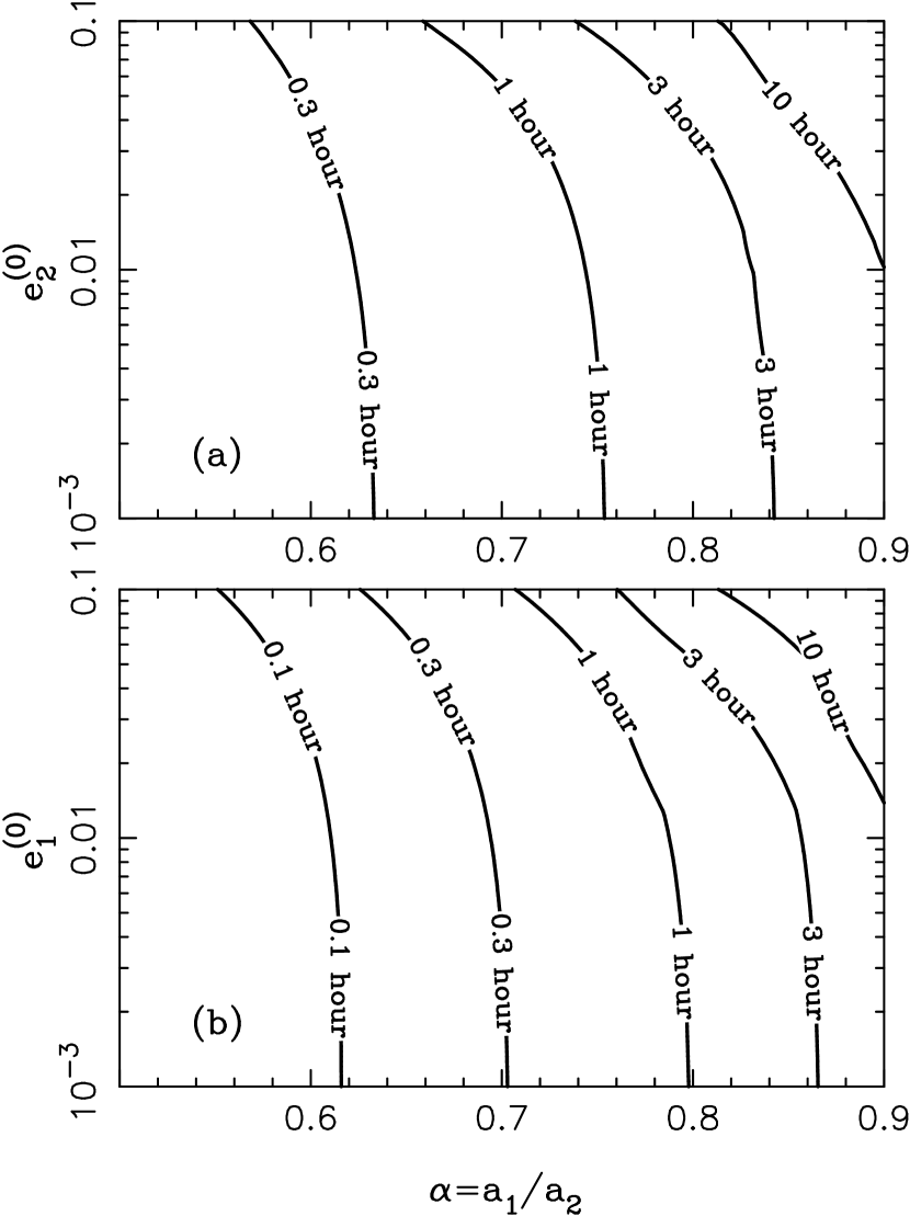
Figure 7: The TTV amplitude of the outer (top panel) and inner (bottom panel) planets. We used $m_{1}=m_{2}=10^{-5}\ M_{*}$, $M_{*}=M_{\odot}$, $a_{2}=1$ AU, and varied $e_{i}^{(0)}$. The inner planet’s semimajor axis was chosen such that $0.5<\alpha<0.9$. The TTV amplitudes are given here for a single conjunction between planets.

Figure 7 shows how the amplitude of the conjunction effect changes with eccentricity. Given that our analytic model loses precision with increasing eccentricity (see Figure 5), here we used our $N$-body code to compute $\delta t_{i}$ over one conjunction cycle. In addition to changing $\alpha$ as in Figure 6, we also varied the initial eccentricities of the two planets. Figure 7 shows that the amplitude of the conjunction effect can increase by a factor of $\simeq 2$-10 by increasing the eccentricity from 0 to 0.1. This is significant, because it shows that the likelihood of detection of the conjunction effect can be boosted for orbits with modest eccentricities, a case that should presumably be common among planetary systems.

The magnitude of the conjunction effect for eccentric orbits, however, also depends on the relative orientation of orbits, as given by $\varpi_{1}$ and $\varpi_{2}$, and on where exactly the conjunction happens along the orbits. The magnitude can increase or decrease, roughly reflecting the physical distance between planets during the conjunction. Figure 7 was produced by surveying all orbital configurations, $0\leq\varpi_{1}<2\pi$ and $0\leq\varpi_{2}<2\pi$, and plotting the one for which the magnitude was maximal.

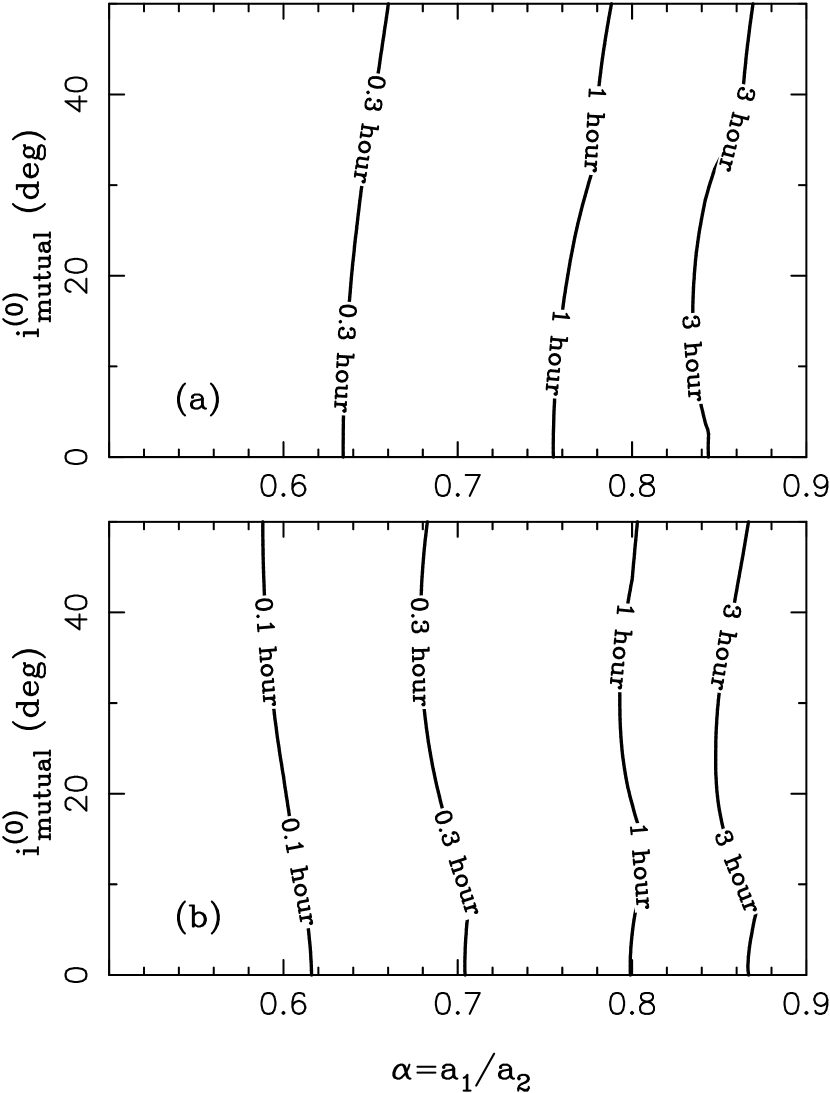
Figure 8: The TTV amplitude of the outer (top panel) and inner (bottom panel) planets. We used $m_{1}=m_{2}=10^{-5}\ M_{*}$, $M_{*}=M_{\odot}$, $a_{2}=1$ AU, $e_{i}=0$ and varied the mutual inclination between the two orbits. The inner planet’s semimajor axis was chosen such that $0.5<\alpha<0.9$. The TTV amplitudes are given here for a single conjunction between planets.

Figure 8 shows how the amplitude of the conjunction effect changes with the mutual inclination between orbits, $i_{\rm mutual}$. As in Figure 7 we used the $N$-body code to compute $\delta t_{i}$ over one conjunction cycle. Figure 7 illustrates that the amplitude of the conjunction effect is not very sensitive to $i_{\rm mutual}$. The magnitude varies only up to $\simeq$20% for $i_{\rm mutual}<50^{\circ}$, relative to to the case with $i_{\rm mutual}=0$. See Nesvorný et al. (2009) for a more general analysis of the dependence of the short-periodic TTVs on orbital inclinations.

5 Discussion

Equations (32) and (33) express our expectation for the TTVs produced by two planets on nearly circular and coplanar orbits. The first two terms in these equations result from the direct perturbation of the mean longitude. If $\alpha$ is sufficiently close to 1, these terms are essentially equivalent to a succession of transit timing discontinuities occurring at orbital conjunctions between planets. The amplitude of these discontinuities is $2A_{1}(\alpha)m_{2}/M_{*}$ for the inner planet and $2B_{1}(\alpha)m_{1}/M_{*}$ for the outer planet, where $A_{1}(\alpha)$ and $B_{1}(\alpha)$ were defined in Eqs. (2.2.1) and (2.2.1) and were illustrated in Figure 6 (dashed lines). The transit times of the inner planet are expected to be delayed relative to a fixed Keplerian ephemeris, while those of the outer planet are expected to be sped up.

The long-term effects of conjunctions, with $\delta t_{i}$ steadily accumulating over many periods of the synodic angle, can be absorbed by a small change of the orbital period. The short-period effects of conjunctions, frequently described as ‘chopping’ of the TTV signal (e.g, Holman et al. 2010, Carter et al. 2012), should not be mistaken with anything else. When the long-term conjunction effects are removed from the transit ephemeris, the TTV signal from direct perturbation of the mean longitude should have a saw-like profile with each tooth being marked by a few rising and a few declining transits. If such a saw-tooth profile is identified in the data, the mass of planetary companion can be extracted from these measurements, assuming that $\alpha$ is known, by using Eqs. (32) or (33). If $\alpha$ is unknown, Eqs. (32) or (33) can be used to constrain $A_{1}(\alpha)m_{2}/M_{*}$ or $B_{1}(\alpha)m_{1}/M_{*}$.

As an example, we discuss the chopping in the TTVs of KOI-884.02 and Kepler-36c (Figure 1). As for Kepler-36, $P_{2}\simeq 16.2$ day, $\alpha\simeq 0.9$, $M_{1}/M_{*}\simeq 1.3\times 10^{-5}$ from Carter et al. (2012). The size of the conjunction step computed from Eq. (34) for these parameters is $\delta t_{2}\sim 0.3$ hour. For a comparison, Figure 1b shows that the actual steps during conjunctions are smaller, but not much smaller, than one hour. As for KOI-884.02, $P_{1}\simeq 20.5$ day, $\alpha\simeq 0.34$, $M_{2}/M_{*}\simeq 3\times 10^{-3}$ from Nesvorný et al. (2012). We compute that $\delta t_{1}\sim 0.9$ hour from Eq. (33). For a comparison, the actual steps in KOI-884.02’s TTVs, best seen for transit cycles between 32 and 45 (Figure 1a), are $\sim$1-2 hours. The difference is probably caused by small but significant orbital eccentricities (Nesvorný et al. 2014).

The oscillatory part of Eqs. (32) or (33) offers a different method to constrain planetary masses and/or $\alpha$. Here it can be useful to perform the Fourier analysis of $\delta t_{i}$. The expectation is that this will reveal frequencies that are integer multiples of $(n_{1}-n_{2})$. Some of these frequencies will be faster than the Nyquist frequency, $f^{\rm N}_{i}=\pi/P_{i}$, and will be aliased to the part of the Fourier spectrum with $f<f^{\rm N}_{i}$. For example, in the test case shown in Figure 4, $f^{\rm N}_{1}=0.01117$ d^-1. Therefore, frequencies $(n_{1}-n_{2})=0.00514$ d^-1 and $2(n_{1}-n_{2})=0.01028$ d^-1 appear unaliased, while all $j(n_{1}-n_{2})$ frequencies with $j\geq 3$ are aliased to $2f^{\rm N}_{1}-j(n_{1}-n_{2})$. For example, $3(n_{1}-n_{2})=0.01542$ d^-1 appears at $0.006933$ d^-1.

As for KOI-884, $(n_{1}-n_{2})=0.201$ d^-1 and $f^{\rm N}_{1}=0.153$ d^-1. As $(n_{1}-n_{2})>f^{\rm N}_{1}$ in this case, the synodic frequency and all its multiples will be aliased. For example, $(n_{1}-n_{2})$ should appear at $0.105$ d^-1, and $2(n_{1}-n_{2})$ should appear at $0.096$ d^-1. The Fourier analysis of the best fit TTV model from Nesvorný et al. (2014) confirms this. It shows that the peak power density of the $2(n_{1}-n_{2})$ term is about five times larger than that of the $(n_{1}-n_{2})$ term, as expected from Eqs. (27) and (33). Unfortunately, these terms are much harder to identify in the existing TTV data of KOI-884.02, because of the short coverage, gaps, measurement errors, and other issues. We have done a similar analysis for Kepler-36, but do not discuss it here, except for pointing out that the aliasing is not a problem for this system, because the synodic frequency $(n_{1}-n_{2})$ is relatively slow (as $\alpha\simeq 0.9$).

Identifying the structure of unaliased and aliased frequencies in the frequency domain can be useful for the interpretation of the TTV observations. As the amplitudes of these terms are proportional to $D_{i}^{j}$, as shown in Eqs. (32) or (33), the TTV measurements can be potentially inverted to obtain a unique determination of the planetary mass and orbital separation (e.g., Nesvorný et al. 2013). This highlights the importance of the conjunction effect.

As a final word of caution, note that Eqs. (32) or (33) were derived under several assumptions. Most importantly, these equations are valid only for small orbital eccentricities. While many planetary systems will presumably fall into this category, perhaps the majority of them will not. The TTVs for planetary systems with orbital eccentricities exceeding the threshold shown in Figure 5 will contain many additional terms from the first and higher eccentricity powers. These terms will add frequencies $k_{1}n_{1}+k_{2}n_{2}$, with arbitrary $k_{1}$ and $k_{2}$, potentially generating resonant or near-resonant TTVs, and will modify the amplitude dependence of the $j(n_{1}-n_{2})$ frequencies on orbital parameters. The analytic model described here therefore cannot be used in general to characterize the planetary systems from TTVs.

The main scientific value of the analytic model is to give us an intuitive framework for how the TTV method works in the limit of the nearly circular orbits.

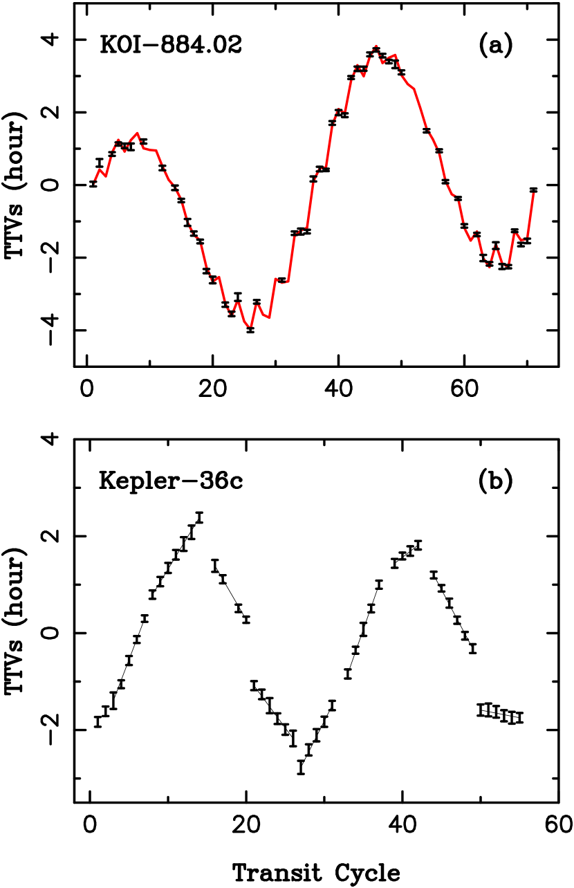
Figure 1: The effect of conjunctions on the TTVs of: (a) KOI-884.02, and (b) Kepler-36c. The TTV data for KOI-884.02 and Kepler-36c were obtained from Nesvorný et al. (2014) and Carter et al. (2012), respectively. The red line in panel (a) shows the best dynamical fit from Nesvorný et al. (2014) corresponding to a (non-transiting) companion with the mass of $\simeq 2.4$ $M_{\rm J}$ and outer orbit just wide the 3:1 orbital resonance with KOI-884.02. The TTVs of Kepler-36c, on the other hand, are caused by a transiting super-Earth (Kepler-36b) with an orbit in the 7:6 resonance with Kepler-36c. The line segments in panel (b) highlight the discontinuous nature of Kepler-36c’s TTVs.

Figure 4: A comparison of the analytic model with numerical integration. The triangles show the actual TTVs obtained from a numerical integration. The solid lines show $\delta t_{i}$ as a function of time, where $\delta t_{i}$ were computed from the analytic model described in Section 2. The differences between analytic and numeric times are shown in the bottom of each panel. These values have to be multiplied by a factor of 60 to appear on the same scale with the upper plots (the dashed horizontal line shows zero for a reference). The two planets have masses $m_{1}=m_{2}=10^{-5}\ M_{*}$ ($M_{*}=M_{\odot}$), semimajor axes $a_{1}=0.84$ AU and $a_{2}=1$ AU (thus $P_{2}/P_{1}\simeq 1.3$), and $e_{i}^{(0)}=0$. The initial mean longitudes were chosen such that $\psi=-\pi$.

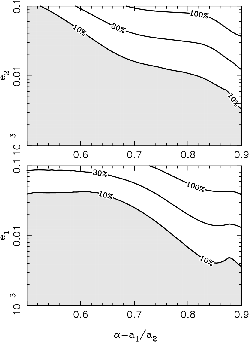
Figure 5: The domain of validity of the analytical model as a function of $\alpha$, $e_{1}$ and $e_{2}$. As in Figure 4, two planets with the mass $10^{-5}\,M_{*}$ each were placed on the initially coplanar orbits. The outer planet was set to have $a_{2}=1.0$ AU and the inner planet’s semimajor axis was varied such that $0.5<\alpha<0.9$. The isolines show the relative precision of the analytic model. The shaded area is where the precision of the analytic model is better than 10%.

Figure 6: The TTV amplitude of the outer (top panel) and inner (bottom panel) planets. The dashed lines show the amplitude of the step-like variation from $\delta\lambda_{i}/n_{i}$ (Eqs. 15 and 19). The solid lines show the total amplitude from $(\delta\lambda_{i}+\delta\lambda_{i}^{\rm eff})/n_{i}$, where $\delta\lambda_{i}^{\rm eff}$ is given in Eqs. (2.2.2) and (27). Here we used $m_{1}=m_{2}=10^{-5}\ M_{*}$, $M_{*}=M_{\odot}$, $a_{2}=1$ AU, and $e_{i}^{(0)}=0$. The inner planet’s semimajor axis was varied such that $0.5<\alpha<0.9$. The TTV amplitudes are given here for a single conjunction between planets.

References

- (1) Agol, E., Steffen, J., Sari, R., Clarkson, W., 2005, MNRAS, 359, 567
- (2) Brouwer, D., Clemence, G. M., 1961, Methods of celestial mechanics, Academic Press, 1961
- Cabrera et al. (2014) Cabrera, J., Csizmadia, S., Lehmann, H., et al. 2014, ApJ, 781, 18
- Carter et al. (2012) Carter, J. A., Agol, E., Chaplin, W. J., et al. 2012, Science, 337, 556
- Deck et al. (2014) Deck, K. M., Agol, E., Holman, M. J., & Nesvorný, D. 2014, arXiv:1403.1895
- Heyl & Gladman (2007) Heyl, J. S., & Gladman, B. J. 2007, MNRAS, 377, 1511
- Holman & Murray (2005) Holman, M. J., & Murray, N. W. 2005, Science, 307, 1288
- Lithwick et al. (2012) Lithwick, Y., Xie, J., & Wu, Y. 2012, ApJ, 761, 122
- (9) Malhotra, R., 1993, ApJ, 407, 266
- (10) Nesvorný, D., 2009, ApJ, 701, 1116
- (11) Nesvorný, D., Morbidelli, A., 2008, ApJ, 688, 636
- Nesvorný & Beaugé (2010) Nesvorný, D., & Beaugé, C. 2010, ApJ, 709, L44
- Nesvorný et al. (2012) Nesvorný, D., Kipping, D. M., Buchhave, L. A., et al. 2012, Science, 336, 1133
- Nesvorný et al. (2013) Nesvorný, D., Kipping, D., Terrell, D., et al. 2013, ApJ, 777, 3
- Nesvorný et al. (2014) Nesvorný, D., Kipping, D., Terrell, D., et al. 2014, ApJ, in press
- Nesvorný et al. (2014) Vokrouhlický, D., Nesvorný, D. 2014, submitted to ApJ