OGLE-ing the Magellanic System: Stellar populations in the Magellanic Bridge

Abstract

We report the discovery of a young stellar bridge, that forms a continuous connection between the Magellanic Clouds. This finding is based on number density maps for stellar populations found in data gathered by OGLE-IV, that fully cover over 270 deg² of the sky in the Magellanic Bridge area. This is the most extensive optical survey of this region up to date. We find that the young population is present mainly in the western half of the MBR, which, together with the newly discovered young population in the eastern Bridge, form a continuous stream of stars connecting both galaxies along $\delta\sim-73.5$ deg. The young population distribution is clumped, with one of the major densities close to the SMC, and the other, fairly isolated and located approximately mid-way between the Clouds, which we call the OGLE island. These overdensities are well matched by HI surface density contours, although the newly found young population in the eastern Bridge is offset by $\sim 2$ deg north from the highest HI density contour. We observe a continuity of red clump stars between the Magellanic Clouds, which represent an intermediate-age population. Red clump stars are present mainly in the southern and central parts of the Magellanic Bridge, below its gaseous part, and their presence is reflected by a strong deviation from the radial density profiles of the two galaxies. This may indicate either a tidal stream of stars, or that the stellar halos of the two galaxies overlap. On the other hand, we do not observe such an overlap within an intermediate-age population represented by the top of the red giant branch and the asymptotic giant branch stars. We also see only minor mixing of the old populations of the Clouds in the southern part of the Bridge, represented by the lowest part of the red giant branch.

1. Introduction

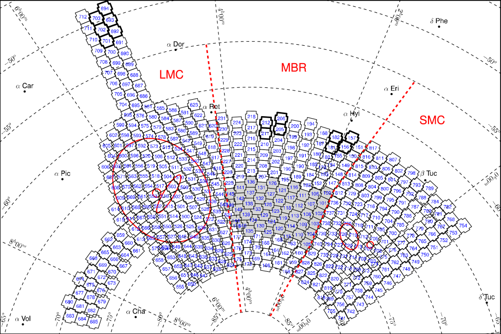
Figure 1.— OGLE-IV fields in the Magellanic Clouds region (approximately 600 deg² of the sky, 1.4 deg² field area). The Magellanic Bridge region ($\sim$270 deg²) is encompassed by red dashed lines and 47 fields of the main part of the Magellanic Bridge ($\sim$65 deg²) are shaded with gray. Fourteen Galactic foreground fields are marked with thick black lines. Large red ellipses mark the location of the LMC (left) and the SMC (right). For a more detailed view of the sky coverage see http://ogle.astrouw.edu.pl/sky/ogle4-fields.html

Table 1OGLE-IV field center coordinates in the Magellanic Bridge region in equatorial and galactic coordinates.

Field	RA [h]	Dec [deg]	l [deg]	b [deg]	Field	RA [h]	Dec [deg]	l [deg]	b [deg]	Field	RA [h]	Dec [deg]	l [deg]	b [deg]
MBR100	1.860	-70.06	295.58	-46.20	MBR144	4.031	-75.00	289.16	-36.57	MBR188	2.333	-63.90	287.81	-50.55
MBR101	1.851	-71.29	296.22	-45.06	MBR145	4.095	-71.92	285.75	-38.04	MBR189	2.583	-69.44	290.39	-45.08
MBR102	1.835	-72.52	296.87	-43.91	MBR146	4.139	-73.15	286.93	-37.22	MBR190	2.583	-68.21	289.41	-46.11
MBR103	1.816	-73.75	297.50	-42.76	MBR147	1.847	-68.83	295.08	-47.38	MBR191	2.583	-66.98	288.40	-47.12
MBR104	1.794	-74.99	298.11	-41.61	MBR148	1.803	-67.60	294.81	-48.62	MBR192	2.583	-65.75	287.35	-48.13
MBR105	1.768	-76.22	298.69	-40.46	MBR149	1.761	-66.37	294.55	-49.87	MBR193	2.583	-64.52	286.25	-49.12
MBR106	2.100	-70.67	294.30	-45.19	MBR150	1.722	-65.14	294.29	-51.11	MBR194	2.583	-63.29	285.11	-50.11
MBR107	2.100	-71.90	294.99	-44.06	MBR151	1.687	-63.91	294.00	-52.35	MBR195	2.833	-70.06	289.41	-43.83
MBR108	2.100	-73.14	295.66	-42.92	MBR152	2.119	-69.45	293.45	-46.26	MBR196	2.833	-68.83	288.35	-44.80
MBR109	2.100	-74.37	296.30	-41.79	MBR153	2.061	-68.22	293.12	-47.51	MBR197	2.833	-67.59	287.26	-45.76
MBR110	2.100	-75.60	296.92	-40.65	MBR154	2.007	-66.98	292.80	-48.76	MBR198	2.833	-66.36	286.12	-46.71
MBR111	2.349	-71.29	293.14	-44.10	MBR155	1.955	-65.75	292.49	-50.02	MBR199	2.833	-65.13	284.95	-47.64
MBR112	2.365	-72.52	293.85	-42.98	MBR156	1.908	-64.52	292.17	-51.27	MBR200	2.833	-63.90	283.74	-48.57
MBR113	2.384	-73.75	294.53	-41.85	MBR157	1.865	-63.29	291.83	-52.51	MBR201	3.083	-69.44	287.49	-43.46
MBR114	2.406	-74.99	295.18	-40.71	MBR158	2.046	-79.91	299.10	-36.69	MBR202	3.083	-68.21	286.33	-44.37
MBR115	2.432	-76.22	295.82	-39.58	MBR159	1.955	-78.67	298.89	-37.93	MBR203	3.083	-66.98	285.13	-45.26
MBR116	2.596	-70.67	291.26	-44.01	MBR160	1.878	-77.44	298.68	-39.17	MBR204	3.083	-65.75	283.89	-46.13
MBR117	2.606	-71.91	292.13	-42.95	MBR161	2.461	-79.29	297.50	-36.80	MBR205	3.083	-64.52	282.62	-47.00
MBR118	2.640	-73.14	292.85	-41.83	MBR162	2.331	-78.06	297.26	-38.08	MBR206	3.083	-63.29	281.30	-47.85
MBR119	2.679	-74.37	293.54	-40.70	MBR163	2.221	-76.83	297.02	-39.35	MBR207	3.333	-70.06	286.81	-42.12
MBR120	2.725	-75.60	294.22	-39.57	MBR164	2.708	-78.06	295.95	-37.52	MBR208	3.333	-68.83	285.59	-42.96
MBR121	2.845	-71.29	290.38	-42.81	MBR165	2.667	-76.83	295.28	-38.64	MBR209	3.333	-67.59	284.34	-43.79
MBR122	2.871	-72.52	291.25	-41.75	MBR166	2.933	-79.91	296.53	-35.62	MBR210	3.333	-66.36	283.06	-44.60
MBR123	2.924	-73.76	291.99	-40.63	MBR167	2.967	-78.67	295.56	-36.58	MBR211	3.333	-65.13	281.73	-45.40
MBR124	2.985	-74.99	292.71	-39.50	MBR168	3.083	-77.44	294.28	-37.35	MBR212	3.333	-63.90	280.37	-46.19
MBR125	3.057	-76.22	293.41	-38.36	MBR169	3.392	-79.29	294.87	-35.33	MBR213	3.583	-69.44	285.04	-41.55
MBR126	3.093	-70.68	288.57	-42.51	MBR170	3.392	-78.06	293.84	-36.24	MBR214	3.583	-68.21	283.75	-42.31
MBR127	3.102	-71.91	289.63	-41.56	MBR171	3.392	-76.83	292.79	-37.14	MBR215	3.583	-66.98	282.42	-43.06
MBR128	3.146	-73.14	290.51	-40.51	MBR172	3.700	-79.91	294.67	-34.31	MBR216	3.583	-65.75	281.06	-43.80
MBR129	3.219	-74.38	291.28	-39.38	MBR173	3.700	-78.67	293.57	-35.15	MBR217	3.583	-64.52	279.67	-44.51
MBR130	3.304	-75.61	292.03	-38.25	MBR174	3.700	-77.44	292.45	-35.97	MBR218	3.583	-63.29	278.24	-45.21
MBR131	3.342	-71.30	287.97	-41.23	MBR175	4.116	-79.29	293.23	-33.84	MBR219	3.833	-70.06	284.66	-40.14
MBR132	3.368	-72.53	289.02	-40.28	MBR176	4.076	-78.06	292.11	-34.66	MBR220	3.833	-68.83	283.33	-40.84
MBR133	3.430	-73.76	289.92	-39.22	MBR177	4.043	-76.83	290.97	-35.47	MBR221	3.833	-67.59	281.97	-41.52
MBR134	3.525	-74.99	290.72	-38.09	MBR178	4.015	-75.60	289.81	-36.27	MBR222	3.833	-66.36	280.58	-42.19
MBR135	3.636	-76.23	291.50	-36.95	MBR179	2.150	-67.60	292.06	-47.86	MBR223	3.833	-65.13	279.17	-42.84
MBR136	3.589	-70.68	286.29	-40.74	MBR180	2.150	-66.37	291.24	-48.96	MBR224	3.833	-63.90	277.72	-43.48
MBR137	3.599	-71.91	287.50	-39.91	MBR181	2.117	-65.14	290.67	-50.15	MBR225	4.083	-70.67	284.43	-38.75
MBR138	3.642	-73.15	288.55	-38.97	MBR182	2.117	-63.91	289.78	-51.25	MBR226	4.083	-69.44	283.07	-39.38
MBR139	3.725	-74.38	289.47	-37.91	MBR183	2.333	-70.06	292.42	-45.22	MBR227	4.083	-68.21	281.69	-40.00
MBR140	3.844	-75.61	290.31	-36.77	MBR184	2.333	-68.83	291.57	-46.30	MBR228	4.083	-66.98	280.28	-40.60
MBR141	3.838	-71.30	285.96	-39.40	MBR185	2.333	-67.59	290.69	-47.37	MBR229	4.083	-65.75	278.85	-41.18
MBR142	3.864	-72.53	287.15	-38.57	MBR186	2.333	-66.36	289.77	-48.44	MBR230	4.083	-64.52	277.39	-41.75
MBR143	3.926	-73.76	288.21	-37.63	MBR187	2.333	-65.13	288.81	-49.50	MBR231	4.083	-63.29	275.91	-42.30
SMC729	1.392	-68.83	298.61	-48.03	SMC739	1.521	-74.37	299.31	-42.48	SMC816	1.506	-64.52	296.14	-52.09
SMC730	1.378	-70.06	299.05	-46.83	SMC740	1.475	-75.60	299.88	-41.30	SMC817	1.481	-63.29	295.91	-53.32
SMC731	1.370	-71.29	299.42	-45.63	SMC808	1.359	-67.60	298.55	-49.27	SMC824	1.144	-79.91	301.99	-37.19
SMC732	1.329	-72.52	299.96	-44.44	SMC809	1.338	-66.37	298.39	-50.50	SMC825	1.144	-78.67	301.85	-38.42
SMC733	1.276	-73.76	300.52	-43.25	SMC810	1.320	-65.14	298.23	-51.73	SMC826	1.144	-77.44	301.72	-39.64
SMC734	1.215	-74.99	301.06	-42.06	SMC811	1.303	-63.91	298.05	-52.97	SMC827	1.560	-79.29	300.47	-37.64
SMC735	1.143	-76.22	301.58	-40.86	SMC812	1.627	-69.45	297.00	-47.15	SMC828	1.520	-78.06	300.30	-38.86
SMC736	1.619	-70.67	297.52	-45.97	SMC813	1.595	-68.22	296.78	-48.38	SMC829	1.487	-76.83	300.13	-40.09
SMC737	1.594	-71.91	298.12	-44.81	SMC814	1.562	-66.98	296.57	-49.62
SMC738	1.560	-73.14	298.73	-43.64	SMC815	1.532	-65.75	296.36	-50.85
LMC535	4.506	-73.62	286.47	-35.62	LMC548	4.533	-66.85	278.67	-38.26	LMC619	4.333	-65.13	277.23	-40.05
LMC536	4.557	-72.38	284.99	-35.96	LMC549	4.568	-65.62	277.11	-38.50	LMC620	4.250	-64.00	276.15	-40.99
LMC537	4.602	-71.15	283.49	-36.27	LMC586	4.785	-63.77	274.34	-37.74	LMC621	4.422	-63.77	275.30	-40.03
LMC538	4.641	-69.92	281.99	-36.56	LMC587	4.806	-62.54	272.78	-37.92	LMC622	4.456	-62.54	273.69	-40.24
LMC539	4.677	-68.69	280.47	-36.84	LMC588	4.825	-61.31	271.22	-38.08	LMC623	4.489	-61.31	272.06	-40.41
LMC540	4.708	-67.46	278.95	-37.09	LMC589	4.600	-64.39	275.54	-38.72	LMC624	4.433	-79.77	293.13	-32.85
LMC541	4.736	-66.23	277.42	-37.33	LMC590	4.629	-63.16	273.96	-38.92	LMC625	4.433	-78.54	291.87	-33.49
LMC542	4.761	-65.00	275.88	-37.55	LMC591	4.655	-61.92	272.38	-39.10	LMC626	4.433	-77.31	290.59	-34.11
LMC543	4.287	-73.00	286.35	-36.74	LMC521	4.216	-74.23	287.86	-36.37	LMC627	4.433	-76.08	289.30	-34.72
LMC544	4.349	-71.77	284.84	-37.09	LMC522	4.447	-74.85	287.95	-35.27	LMC628	4.733	-79.15	292.02	-32.43
LMC545	4.403	-70.54	283.31	-37.42	LMC616	4.300	-68.83	281.66	-38.66	LMC629	4.733	-77.92	290.70	-32.97
LMC546	4.452	-69.31	281.77	-37.72	LMC617	4.300	-67.59	280.24	-39.20	LMC630	4.733	-76.69	289.37	-33.50
LMC547	4.495	-68.08	280.23	-38.00	LMC618	4.333	-66.36	278.70	-39.55	LMC631	4.733	-75.46	288.03	-34.01
LMC692	5.187	-51.47	258.51	-36.26	LMC694	5.194	-49.00	255.46	-36.19	LMC702	5.317	-50.85	257.76	-35.04
LMC693	5.191	-50.23	256.98	-36.23	LMC701	5.317	-52.08	259.26	-35.06	LMC703	5.317	-49.62	256.26	-35.01

The Magellanic Clouds (MCs) comprise of two galaxies: the Large and the Small Magellanic Cloud (LMC and SMC, respectively), and are the closest to the Milky Way (MW) pair of interacting galaxies. The Clouds have always been of special interest to astronomers and they continue to play a significant role in our understanding of the Universe.

There exists irrefutable evidence that the MCs interact with each other and with our Galaxy (e.g. Besla et al. 2012, Diaz & Bekki 2012): the Magellanic Bridge – a stream of gas and stars between the MCs; the Magellanic Stream – $160$ deg long stream of gas trailing the MCs on their orbit around the MW; the Leading Arm – a stream of gas leading the MCs on their orbit. The Magellanic Clouds and all the structures described above are collectively called the Magellanic System.

The Magellanic Bridge (hereafter MBR) has long been known to contain neutral and ionized gas (Mathewson & Ford 1984, Marcelin et al. 1985, Putman 2000, Muller et al. 2003, Barger et al. 2013) connecting the MCs. It is widely believed that gas present in the MBR has been drawn out of the SMC through tidal forces, during the most recent encounter of the two galaxies, that took place 200 Myr ago (Mathewson 1985, Muller et al. 2004). Observations of young stars on the SMC side of the Bridge, whose age estimates are consistent with 200 Myr, support this hypothesis (Irwin et al., 1985).

Early observations of the MBR also revealed a young stellar counterpart in the Shapley Wing of the SMC (Shapley 1940, Meaburn 1986, Courtès et al. 1995) and in a number of locations between the Clouds (Irwin et al. 1990, Grondin et al. 1992, Demers & Battinelli 1998).

Harris (2007) searched for older stellar populations that should have been drawn out of the SMC by those same tidal forces that drew out gas, in a dozen fields uniformly sampling the Bridge, most following the ridge-line of neutral hydrogen ($\delta\sim-74$ deg) and two slightly off. He did not find any signs of older populations, suggesting, that maybe all stars present in the MBR formed there, and for some reason tidal forces stripped just pure gas from the SMC.

Recently, Bagheri et al. (2013) used near infrared public data from 2MASS (Two Micron All Sky Survey) and WISE (Wide-Field Infrared Survey Explorer) for the MBR region, spanning 8 deg in declination. They analyzed color-magnitude and color-color diagrams and found traces of an older population of stars, estimated to be somewhat between $\sim 400$ Myr and 5 Gyr old. However, the exact age and the MBR membership of these stars need to be confirmed by further observations.

Another study of the Bridge region was carried out by Nöel et al. (2013), as a part of the MAGellanic Inter-Cloud program (MAGIC). They used observations from two fields between the Clouds, of total area of $1.12$ deg². With a synthetic color-magnitude diagram fitting technique they showed that 28% of stars in observed regions are intermediate age and that there are also hints of an older population, that might have been tidally drawn out of the SMC. However, spectroscopic observations are needed to confirm or rule out their SMC origin.

Most recently, Nidever et al. (2013) investigated the spatial distribution of red clump stars in the vicinity of the SMC. They found, that the eastern side of the SMC has a large line-of-sight depth, which shows a distance bimodality, with one component being closer to us than the “systemic” SMC distance. The authors argue that this population is a stellar counterpart of the gaseous MBR, that was stripped from the SMC $\sim$200 Myr ago. However, their data were not well reproduced by the MCs simulations, which suggests, that the simulations need to be revised to take into account the larger extent of stellar components in the MBR.

There is also an on-going survey of the SMC and the MBR performed with the ESO VLT Survey Telescope, called STEP (the SMC in Time: Evolution of a Prototype interacting late-type dwarf galaxy). The survey will cover 74 deg² of the sky with multiple filters to magnitudes fainter than the Main Sequence turn-off (Ripepi et al., 2014).

Regarding the Magellanic System simulations, we have to mention here, that even though there is an agreement, that gaseous features on the Magellanic System are an effect of some form of interactions between the SMC, LMC and the MW, there is still an ongoing debate on the nature of these interactions. One popular scenario is that the gaseous features of the Magellanic System were created during multiple pericentric passages of the MCs on their orbit around the MW, either via tidal effects or ram pressure stripping (see the summary by Ruzicka et al. 2009). Another possibility is that the LMC and SMC have become an interacting pair only recently, with a first close encounter $\sim$2 Gyr ago and a second $\sim$250 Myr ago. In the light of recent proper motion measurements based on HST data (Kallivayalil et al., 2013), it is highly probable that the MCs are either on their first infall into our Galaxy or on an eccentric, long period orbit around the Galaxy (Besla et al., 2007), and have been a bound pair for past couple of Gyr. Regarding the MBR, Besla et al. (2012) argue, that the internal kinematics and structure of the Clouds suggest that there was a recent direct collision ($\sim 200$ Myr ago) of the MCs, that produced the Bridge and triggered star formation within it. This is consistent with simulations of Diaz & Bekki (2012), which show that the MBR was formed due to a strong tidal interaction $\sim$250 Myr ago.

The Optical Gravitational Lensing Experiment (OGLE) is a long-term large scale sky survey focused on variability studies of dense stellar regions. The OGLE project started regular observations in 1992 as one of the first generation microlensing projects dedicated to detecting and characterizing microlensing events (Udalski et al., 1992). During its over 22 year history OGLE gradually evolved and conducted numerous projects that contributed to many fields of modern astrophysics. The current, fourth phase of the OGLE survey (OGLE-IV) started in March 2010 with the commissioning of a large new generation 256 Megapixel 32-chip mosaic camera. The Galactic bulge and disk, the Magellanic Clouds, and the Magellanic Bridge, including vast areas around them, are the primary observing targets for the OGLE-IV survey.

In this paper we present density maps of stellar populations in the entire Magellanic Bridge region, thanks to the unprecedented OGLE-IV coverage. The maps show, for the first time, the detailed extent of these populations, which should provide valuable input information for models of past MW and MCs interactions.

2. Observations and Data Preparation

2.1. OGLE-IV Observations

Regular monitoring of the selected sky regions by the OGLE survey is carried out with the 1.3 m Warsaw telescope located at the Las Campanas Observatory in Chile (operated by the Carnegie Institution for Science) equipped with the 256 Megapixel 32-chip mosaic camera. The field of view of the camera is $1.4$ square degrees and a pixel size is $\sim 0\farcs 26$. The magnitude range of the standard OGLE survey is approximately $12-21$ mag in the $I$ band and $12.5-21.5$ mag in the $V$ band.

Figure 1 shows OGLE-IV coverage of the Magellanic System. Shaded MBR fields ($1^{h}40^{m}\lesssim\alpha\lesssim 4^{h}15^{m},-77^{\circ}\lesssim\delta\lesssim-70^{\circ}$) have been observed since 2010, while uncolored MBR fields (additional $\sim 3$ deg south and $\sim 7$ deg north in $\delta$) since 2012. Number of epochs is on average $280$ in $I$ and $20-36$ in $V$ for the shaded region and $85$ in $I$ and $3-13$ in $V$ for the rest of the MBR. In this paper we analyze the entire MBR region, as well as two-field wide stripes on both the SMC and the LMC side. We also use additional 6 fields north of the LMC which, together with 8 northern MBR fields, will be used as a Galactic foreground representation (marked with thick black lines in Figure 1). The list of field center coordinates is given in Table 1.

2.2. Data Reduction

OGLE observations are reduced on site at the telescope and the photometry is done in real time. After standard bias subtraction and flat-fielding (sky flats), images are processed with the OGLE photometric data pipeline (Udalski, 2003) that is based on image subtraction using the “difference image analysis” technique software (DIA, Wozniak 2000) adapted to OGLE data (Udalski et al., 2008). In the first step a reference image for each field is constructed from 3–6 good quality frames. Then each frame is aligned with the reference image for that field and the reference image is scaled to match the PSF (point spread function) and background of this frame. In the last step the reference image is subtracted from the frame, leaving a difference image with flux only from those objects that either brightened or dimmed.

The database of all sources is created from the reference images with DoPHOT (Schechter et al., 1993) that identifies sources and measures their mean magnitudes. The light curves are made by adding (or subtracting) the flux from a difference image to the flux from the reference image. Finally, data are calibrated to the standard Johnson-Cousins photometric system and the positions of stars are transformed to equatorial coordinates (Szymański et al., 2011).

The final photometric database contains 12 million objects (in $I$) in the entire analyzed Bridge region (both the MBR and LMC/SMC strips), ranging from 25,000 objects per field in sparse areas and 500,000 objects per field in dense areas close to the LMC.

2.3. Data cleaning

After basic reductions described in the previous subsection, we make several cuts to the data to obtain a clean, homogeneous sample of the MBR stellar population. The main source of contamination are detections of spurious sources located within spikes and halos from saturated stars, ghost reflections from nearby bright objects, as well as multiple detections on extended objects, etc. We identify those in two ways: by their light curve scatter and proximity of similarly looking objects.

We start by assuming that all sources are spurious detections. For each source the algorithm counts the number of neighbors within 10, 15, and 20 pixel radii and remembers their magnitudes. Then a series of conditions are tested which, if true, change the status of a source to a real detection. First: an object has at least two neighbors within $r=20$px and all of them are fainter than the object, and the sum of the magnitude differences between this object and each of the neighbors is greater than some factor $C$ times the number of the neighbors, i.e.

$$\sum_{i=1}^{n}\left(m_{obj}-m_{i}\right)>C\times n$$

In our case $C$ was empirically chosen to be equal to 2/3. This condition identifies large concentrations of similar-brightness detections, such as found around bright stars or extended objects, leaving the brightest of them (e.g. the actual bright star center). Second: an object does not have any neighbors within $r=15$px or has one neighbor within $r=15$px and none within $r=10$px. This condition ensures that isolated stars are not rejected. Third: an object has no more than two close neighbors (within $r=20$px). If none of the above conditions are true, and object stays marked as a spurious detection candidate. If at least one condition is true, an object is marked as real. These criteria are a result of extensive analysis and visual investigation of many images. The described method works well in uncrowded fields such as those in the MBR and the false positives (negatives) fraction is less than 1%.

In the second step, for each object, we compare measurement errors of individual observations in the object’s light curve as well as the scatter of observations around the mean magnitude value for this star, with the same two parameters for a typical star of this magnitude. This allows for identifying ghost reflections, spikes from bright stars and other spurious objects, because they typically vary a lot from epoch to epoch, due to differences in telescope pointing, as well as seeing and background levels. Having access to light curves of all objects in our database, we can calculate a typical rms scatter for a light curve at a given magnitude, ${\rm rms}_{\rm m}$, in the entire magnitude range. Having done that, each star is assigned a $\Delta_{\rm scatter}$ value which tells how different its light curve scatter is from ${\rm rms}_{\rm m}$, in units of Gaussian standard deviations. The same procedure is done for photometric uncertainties of individual measurements reported by the pipeline, so that real variable stars are not rejected from the database – since spurious detection often do not have regular PSFs, the photometric pipeline tends to assign measurement errors higher than typical for a star of a given magnitude. Each star is assigned a $\Delta_{\rm error}$ value which tells us how atypically high mean uncertainties in its light curve are. When $\Delta_{\rm scatter}\times\Delta_{\rm error}>64$, an object is marked as spurious. If $\Delta_{\rm scatter}\times\Delta_{\rm error}>9$, we check if there are any other objects suspected spurious within 20 px radius, and if this is the case, we mark the object as spurious.

Lastly, if an object is marked as a spurious detection candidate by both algorithms, we reject it from the final database.

Figure 2.— Luminosity functions for 47 fields that cover the main MBR. The top panel shows data before removing spurious detections and the bottom panel after the cleaning (for details refer to Section 2.3). Dotted lines mark the bright and faint completeness limits.

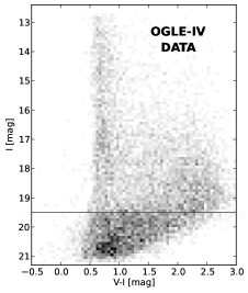
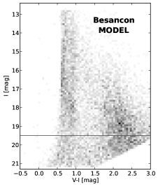
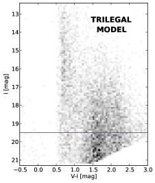
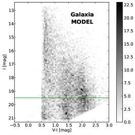
Figure 3.— Hess diagrams of LMC694 – one of the OGLE-IV Galactic fields. The left panel shows real OGLE-IV data, while the middle and right panels show Galaxy simulations of the same area on the sky, based on Besançon, TRILEGAL and Galaxia models, respectively. Bin sizes are 0.1 mag in $I$ and 0.05 mag in $V-I$. The color of each bin corresponds to the number of stars in that bin, as indicated on the color bar on the right. The horizontal line at $I=19.5$ mag is drawn to focus attention on the upper part of the diagrams, which should be almost unaffected by noise.

Next we construct a luminosity function for each field to find data completeness limits. In Figure 2, we plot luminosity functions of all 47 MBR fields (both panels). The top panel shows data before the cleaning process described above and the bottom panel shows data after the cleaning. We see that the luminosity function shape changed for $19<I<21$. A small bump around 20.5 mag (top panel), which was mainly due to spurious detections around bright stars, has almost disappeared, although not completely, as the uncertainty whether an object is real or not, grows quickly at faint magnitudes. The bump at $I=18.2$ mag is the red clump present in some MBR fields, and the bump at $I=22.5$ mag is mostly due to cosmic rays that had not been removed by the pipeline. We choose $I$ band magnitudes of 12.8 and 21.2 as the bright and faint completeness limits for our sample, keeping in mind that the faint end of the luminosity function is contaminated by spurious detections.

As can be seen in Figure 1, a number of OGLE-IV fields overlap resulting in multiple detections in those regions. The detection is considered multiple if the distance between objects is $\leq 0\farcs 52$ (equivalent of 2 OGLE pixels). We remove those duplicate objects in a way that we keep the one that has more epochs, or, if the number of epochs is similar (within $10\%$), has the lower light curve errors.

The Magellanic Bridge region contains numerous globular and open clusters. We use the most recent catalog of the Magellanic System clusters (Bica et al., 2008) as a reference to identify all clusters lying within OGLE-IV fields (189 clusters) and we remove them from the final sample using the mean value of both dimensions as a cluster diameter.

After all cleaning steps described above, the database is reduced from 12 to 5 million sources (from 5 to 2.5 million sources for stars brighter than $I=20$ mag).

2.4. Extinction Correction

Extinction toward the Magellanic Bridge is generally small. Dust extinction maps from Schlegel et al. (1998) give $E(B-V)$ values in the range 0.02–0.15 mag with the mean value of 0.06 mag. This translates to $E(V-I)$ between 0.03–0.19 mag and the mean of 0.08 mag. Galactic foreground fields were chosen to have very low color excesses, with $E(V-I)$ not exceeding 0.04 mag. We correct both the MBR and the calibration fields for extinction using Schlegel et al. (1998) extinction tables obtained from the NASA/IPAC Infrared Science Archive with the spatial resolution of 0.05 deg.

2.5. Galactic Foreground Removal

The Galactic foreground contribution can be accounted for by subtracting a Galactic Hess diagram from a Hess diagram of the science field. This requires either having observations of a purely Galactic field that correspond to the science data in terms of location, magnitude and color range, and completeness (ideally from the same telescope), or creating a Galaxy model with adequate parameters for an area that needs to be cleaned, e.g. the widely used Besançon Model of stellar population synthesis of the Galaxy (Robin et al., 2003), or TRILEGAL (Girardi et al., 2005), or a new promising tool Galaxia (Sharma et al., 2011) that combines the advantages of the Besançon and TRILEGAL Galaxy models.

On the other hand, there are a number of fields within OGLE-IV sky coverage suitable as a Galactic foreground representation. We chose the ones marked with thick lines in Figure 1. They constitute three groups in terms of Galactic latitude: six far LMC fields (LMC692-LMC694, LMC701-LMC703) at $b\approx-36^{\circ}$, four MBR fields (MBR205, MBR206, MBR211, MBR212) at $b\approx-47^{\circ}$ and four MBR fields (MBR156, MBR157, MBR181, MBR182) at $b\approx-52^{\circ}$. These fields lie far from both galaxies and any known dust regions, and their Galactic latitudes cover the latitude range of the investigated region (all coordinates are listed in Table 1), so they should be a good representation of the Galactic population. The left panel in Figure 3 shows a Hess diagram of one of those fields (LMC694). For comparison, the middle and right panels show Hess diagrams of three Galaxy models generated for the same area that is covered by field LMC694, using standard model parameters of Besançon, TRILEGAL, and Galaxia Galaxy models (downloaded from http://model.obs-besancon.fr/, http://galaxia.sourceforge.net/ and http://stev.oapd.inaf.it/cgi-bin/trilegal), respectively. As expected, data-based CMD is a good representation of the Galactic population and does not show any features characteristic of the nearby galaxies (e.g., the main sequence or the red giant branch populations), hence we will further use it for the Galactic foreground removal, instead of Galaxy models presented above.

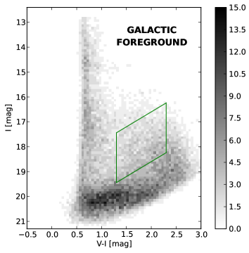
Figure 4.— Average combined Hess diagrams of the six Galactic OGLE-IV fields (LMC692-LMC694 and LMC701-LMC703). Bin sizes are 0.1 mag in $I$ and 0.05 mag in $V-I$. The color of each bin corresponds to the number of stars in that bin, as indicated on the color bar on the right. Green rhomboid marks the region used for scaling the diagram before it is subtracted.

We create OGLE data-based Galactic Hess diagrams by average-combining six/four fields within each of the three Galactic foreground groups (in order to reduce pixel noise) and use those as a Galactic foreground representation (see Figure 4). For each science Hess diagram, we choose a foreground diagram that is closest to it in terms of $b$ and use it for Galactic foreground subtraction. When subtracting, we scale the Galactic Hess diagram such that it contains the same number of stars as the science diagram, in an area that is expected to consist of the Galactic population only. We choose this CMD region to be enclosed with a set of lines: $V-I>1.3$; $V-I<2.3$; $I<-1.2\times(V-I)+21$; $I>-1.2\times(V-I)+19$ (green rhomboid in Figure 4). This should account for incompleteness in the observational data.

As a side test, we also subtracted Besançon, TRILEGAL and Galaxia Hess diagrams from science Hess diagrams for a number of MBR fields, using Galaxy models generated at those exact locations. We then compared the $\chi^{2}$ of all subtractions (data, Besançon, TRILEGAL, and Galaxia) in the CMD region occupied by the Galactic population. We found the $\chi^{2}$ values to be about twice as large for the models subtractions as compared to the data subtractions. This additionally supports the use of the far LMC and MBR fields as a data-based Galactic foreground representation, instead of a model-based one.

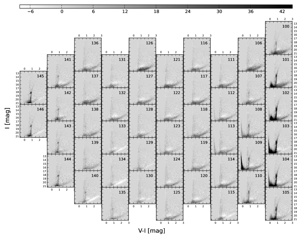
Figure 5.— Hess diagrams of the main part of the Magellanic Bridge region, after removing the Galactic foreground contribution. Figure panels are arranged to reflect OGLE-IV field location in the sky, such that the LMC is to the left and the SMC is to the right (compare with Figure 1). Each panel presents a CMD of the entire OGLE-IV field. Bin sizes are 0.1 mag in $I$ and 0.05 mag in $V-I$. The color of each bin corresponds to the number of stars in that bin, as indicated on the color bar at the top of the figure.

3. Results and Discussion

3.1. Color–Magnitude Diagrams

Figure 5 shows Galaxy-subtracted Hess diagrams of 47 fields in the main part of the Bridge region (fields MBR100 – MBR146). Figure panels are arranged in a way that reflects each field’s location on the sky (compare with Figure 1). For the majority of presented fields there is a region of over-subtraction at $I\sim 20$ mag and $V-I$ between $1-2$ mag, and a region of under-subtraction below it, which are caused by a lower magnitude limit of the Galactic fields as compared to the MBR fields (due to a smaller number of observations).

The young population (YP, $V-I\lesssim 0$) is very prominent on the SMC side and fades as we look further into the MBR, reaching about half way in the central part (field MBR123). This is consistent with previous findings (e.g. Harris 2007), but the exact extent and density distribution of the YP across the Bridge have not been known so far. Older and intermediate-age populations, i.e. red giant branch (RGB) and red clump (RC) stars, respectively, are present on both the LMC and the SMC side, and what we see is most probably the extent of these galaxies into the MBR. Interestingly, the shape of the RC distribution on the CMD is round on the LMC side and vertically elongated on the SMC side. This elongation is caused by a large line-of-sight depth, rather than a presence of blue loops stars, as shown by Nidever et al. (2013).

We will discuss the population distributions in greater detail in the following sections.

3.2. Population Selection Regions

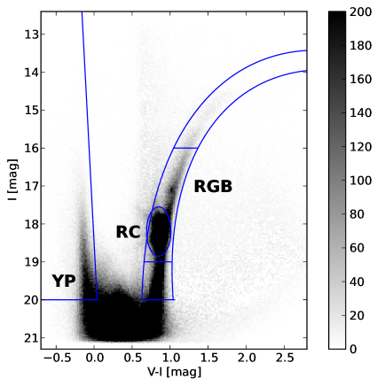
Figure 6.— Cumulative Galaxy-subtracted Hess diagrams of a number of fields in the MBR. Lines mark regions occupied by the young population (YP), RC and RGB stars. Line equations are: $I\geq 38\times(V-I)+18.5$, and $I\leq 20$ for the YP; $(V-I-0.85)^{2}/0.16^{2}+(I-18.2)^{2}/0.65^{2}\leq 1$ for the RC; $(V-I-4.5)^{2}/3.5^{2}+(I-24.9)^{2}/11.6^{2}\leq 1$, $(V-I-4.5)^{2}/3.1^{2}+(I-23.1)^{2}/9.3^{2}\geq 1$, and $V-I\leq 3.0$, and $I\leq 20$ for the RGB stars. RGB stars are further subdivided into top, middle and bottom part at $I=19$ and $I=16$ mag. To increase resolution binning has been reduced to 0.04 mag in $I$ and 0.02 mag in $V-I$. As in previous figures, the color of each bin corresponds to the number of stars in that bin, as indicated on the color bar on the right.

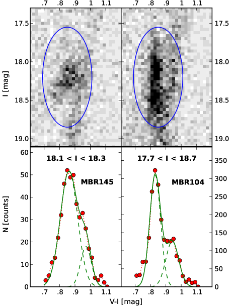
Figure 7.— A comparison of elongated and compact RC for two fields on the opposite sides of the Bridge: MBR104 (left, close to the LMC) and MBR145 (right, close to the SMC). To increase resolution binning has been reduced to 0.04 mag in $I$ and 0.02 mag in $V-I$. Top panels show Galaxy-subtracted Hess diagrams of the RC region. Bottom panels show $V-I$ histograms for the same fields, where the data have been summed along the magnitude axis within the range indicated on the images. Green solid line shows a two Gaussian fit to the data (red dots), while green dashed lines show each of the two Gaussian distributions.

Selection regions for the three main stellar populations (YP, RC, and RGB) are shown on a Hess diagram in Figure 6, with line equations in the figure caption. To avoid contamination from stars belonging to the main sequence of the two galaxies, we set a limit $I<20$ mag for all groups. The RC ellipse is strongly elongated to include all RC stars in fields that have a large line-of-sight depth. As shown by Nidever et al. (2013) for the SMC periphery, this is strictly a distance effect and does not indicate a presence of blue loop stars. A region occupied by RGB stars was further subdivided into top ($I<16$ mag), middle ($16<I<19$ mag), and bottom ($I>19$ mag) parts to separate asymptotic giant branch (AGB) and younger RGB stars (top RGB region) stars from old, low-mass stars (bottom RGB region).

Areas occupied by the RC and the RGB stars overlap significantly and this has to be taken into account when extracting RC and middle RGB groups from the sample. In order to separate these populations we divide the RC ellipse into two regions in $V-I$. Stars bluer than the separation value are included into the RC population, while stars redder than the separation value are included into the RGB population. Top panels of Figure 7 show close-ups of the RC region in the Hess diagrams of two exemplary fields lying on the opposite sides of the Bridge (MBR104 and MBR145), one having an elongated RC and the other a compact RC. Bottom panels show $V-I$ histograms of those close-ups, where for each $V-I$ value data were summed over a range of magnitudes covering the RC (indicated on the images). As an attempt to determine a separation value mentioned above, we fit a function composed of two Gaussian distributions to the summed histograms. The fits are plotted with green lines in Figure 7. In the case of field MBR104 (elongated RC), the fit yields: $\mu_{(V-I),RC}=0.83\ \rm{mag}$, $\sigma_{(V-I),RC}=0.04\ \rm{mag}$, and $\mu_{(V-I),RGB}=0.94\ \rm{mag}$, $\sigma_{(V-I),RGB}=0.04\ \rm{mag}$, and the Gaussian cross at $V-I\approx 0.89$ mag. In the case of field MBR145 (compact RC), the fit results are: $\mu_{(V-I),RC}=0.86\ \rm{mag}$, $\sigma_{(V-I),RC}=0.06\ \rm{mag}$, and $\mu_{(V-I),RGB}=0.97\ \rm{mag}$, $\sigma_{(V-I),RGB}=0.04\ \rm{mag}$, and the Gaussian cross at $V-I\approx 0.94$ mag. We adopt the crossing point of the two functions as a separation value between the RC and the RGB, within the ellipse surrounding the RC region. Outside this ellipse, we use the regions as shown in Figure 6.

Using a single crossing point as a separation between the RC and the RGB is a rough estimation that does not take into account the fact that the overlap fraction of the RC and the RGB changes when moving along the $I$ axis, due to an inclination of the RGB. However, this value is averaged over the magnitude range covering the whole overlap, which is larger than average at fainter magnitudes and smaller at brighter magnitudes. So if the densities within each population do not change very differently with magnitude over this magnitude range, an average value should be a sufficient approximation.

3.3. Two-dimensional Density Maps

In the last step before we construct density maps, we subdivide all data into smaller regions (in right ascension and declination) to increase the spatial resolution of the maps. We chose a 0.335 deg² square subfield (instead of 1.4 deg² OGLE-IV field) as a compromise between better spatial resolution and good count statistics of individual Hess diagrams.

Figures 8, 9, 11, and 13 show spatial density maps of the YP, RC and RGB stars in the region covering the whole MBR and two-field wide stripes of the LMC and the SMC adjacent to the MBR. All maps are drawn using a Hammer equal-area projection centered at $\alpha=3.3$ h and $\delta=-70$ deg. The color-coded value of each “pixel” is a logarithm of the number of stars per square degree area, while each “pixel” area is approximately $0.335\deg^{2}$. This value has been corrected for the OGLE data completeness factor, which originates from gaps between OGLE-IV fields, as well as from horizontal and vertical gaps between the 32 chips in the OGLE-IV camera. The completeness factor also takes into account masked regions around bright stars and stellar clusters. It varies between 80% and 98% for a typical subfield, with a mean value of 93%, but can be as low as a few percent, if the subfield happened to fall close to one of the larger gaps between fields.

The maps also show an approximate location of the LMC disk and the main stellar body of the SMC, marked with white ellipses at $\alpha=05^{\rm h}29^{\rm m}$, $\delta=-69^{\circ}30^{\prime}$ (LMC), and $\alpha=00^{\rm h}54^{\rm m}$, $\delta=-72^{\circ}57^{\prime}$ (SMC). The white cross marks the SMC center of the outer SMC population found by Nidever et al. (2011) at $\alpha=01^{\rm h}00^{\rm m}31^{\rm s}$ and $\delta=-72^{\circ}43^{\prime}11^{\prime\prime}$.

A full list of all number densities for the YP, RC and RGB stars together with their coordinates is available on-line from the OGLE website http://ogle.astrouw.edu.pl, and a few exemplary lines are listed in Table 2.

3.3.1 The Young Population

Figure 8 shows a density map of the young ($\lesssim 1$ Gyr) population, where only $\geq 2\sigma$ detections have been plotted. Color contours mark a number of neutral hydrogen (Hi) emission levels. The Hi emission was integrated over the velocity range 80 ¡ v ¡ 400 km/s, where each contour represents the Hi column density twice as large as the neighboring contour. Hi column densities are in the range $10^{20}-4\times 10^{21}{\rm cm}^{-2}$. Data were taken from the LAB survey of Galactic Hi (Kalberla et al., 2005).

We see that the YP is present mainly in the western part of the main MBR ($\alpha\leq 3$ h), which is consistent with previous findings (Irwin et al. 1985, Irwin et al. 1990, Demers & Battinelli 1998, Harris 2007) and simulations (Besla et al., 2012). However, we discover that there is a non-negligible young population in its eastern part, in the direction of the LMC ($3\lesssim\alpha\lesssim 4.2$ h, $-74\lesssim\delta\lesssim-73$ deg), at the level of 25-90 stars/deg², which is significantly higher than the median background level estimated from 40 most southern fields to be 1 star/deg² with a standard deviation of 6 stars/deg², meaning that these are $4-14\sigma$ detections. This is the first time that the YP is seen in the eastern Bridge, thus showing that there is a continuous stream of young stars connecting the two galaxies.

It is also worth noting that preliminary search for pulsating stars in the main MBR area resulted in the discovery of four short period classical Cepheids distributed along eastern and central parts of the bridge, which is reassuring. A more detailed analysis of pulsating stars in the MBR will be published in the forthcoming papers.

We also show details of the YP distribution within the MBR, which was not possible before, as there was no optical survey that fully mapped the entire region. We can clearly distinguish two major overdensities in the western MBR, one closer to the SMC at $\alpha\approx 2$ h and $\delta\approx-74$ deg, and the other, approximately mid-way between the Clouds at $\alpha\approx 2.9$ h and $\delta\approx-73.5$ deg. We call the latter an “OGLE island” since it is fairly isolated from the main YP part in the MBR. Both overdensities correspond well to the yellow and green Hi contours, and the shape and density distribution of the OGLE island is surprisingly well matched by the shape of the overplotted Hi density contour, showing that star formation was indeed most effective in areas of high Hi surface densities. Interestingly, the gap between the OGLE island and the main part of the YP is not reflected by accordingly lower Hi surface density.

Table 2Number densities for three stellar populations: the young population (YP), the red clump (RC), and the red giant branch (RGB) stars.

$\alpha$	$\delta$	$l$	$b$	YP	RC	RGB top	RGB mid	RGB bottom
[h]	[deg]	[deg]	[deg]	[stars/deg2]	[stars/deg2]	[stars/deg2]	[stars/deg2]	[stars/deg2]
1.3007	$-77.937$	301.145	$-39.099$	26	279	50	536	418
1.3171	$-76.661$	300.848	$-40.355$	45	773	65	851	698
1.3299	$-75.385$	300.545	$-41.612$	253	2448	185	2530	2111
1.3398	$-74.109$	300.234	$-42.867$	3902	4974	299	4820	3913
1.3615	$-79.988$	301.289	$-37.044$	7	171	48	301	211
…	…	…	…	…	…	…	…	…

Note. — Median background levels are $1\pm 6$ stars/deg² for the YP, $36\pm 25$ stars/deg² for the RC, $16\pm 12$ stars/deg² for the top RGB, $63\pm 45$ stars/deg² for the middle RGB, and $112\pm 65$ stars/deg² for the bottom RGB region. A full version of this table, containing number densities in all 754 subfields in the Magellanic Bridge region is available on-line from the OGLE website http://ogle.astrouw.edu.pl.

The eastern part of the young population is not as well matched by the Hi density contours as the western part – it seems that the stars follow the northern edge of the contours more than the southern, and appear to be a continuation of the OGLE island toward the LMC along $\delta\approx-73.5$ deg. Harris (2007) found that the eastward extent of the YP is truncated at $\alpha\simeq 3$ h, but this can be attributed to his sparse field distribution in the MBR that could miss areas of higher stellar densities. On the other hand, Harris (2007) noted that his result is consistent with the fact that the Hi surface density in the eastern Bridge falls below the critical threshold for star formation of about $5\times 10^{21}{\rm cm}^{-2}$ (Kennicutt, 1989). This would imply either that the stars we see were not formed in this area or that the Hi surface density in the past was in fact sufficient for a star formation episode.

3.3.2 The Intermediate-Age and Old Populations

Since our CMDs do not reach the main sequence turn-off, we are unable to resolve age-metallicity degeneracies and estimate ages of observed populations – isochrone fitting for fields closer to the MCs is consistent with populations as old as 13 Gyr and as young as 1 Gyr. In such case we will use red clump stars (ages $\sim$1 to a few Gyr), and the top part of the red giant branch that contains young RGB and AGB stars (ages $\sim 500$ Myr to a couple Gyr), as tracers of an intermediate-age population. The bottom part of the RGB contains oldest stars that only started evolving off the Main Sequence and we will use this group as a tracer of an old stellar population in the Magellanic System. Figures 9 and 11 show density maps of the RC and the top of the RGB, respectively, that represent an intermediate-age population. Figure 13 shows a density map of the bottom part of the RGB that should contain mostly an old population. All maps show detections $\geq 2\sigma$ only.

The RC number density map shows that intermediate-age stars are fairly concentrated around the MCs, although there is a distinct asymmetry in the central and southern part of the map (Figure 9), where the two populations overlap. In Figure 10, we plot number densities of RC stars as a function of distance from the LMC/SMC center (left/right panels), which in the case of the LMC is $\alpha=05^{\rm h}29^{\rm m}$ and $\delta=-69^{\circ}30^{\prime}$ (van der Marel, 2001) and in the case of the SMC is $\alpha=01^{\rm h}00^{\rm m}31^{\rm s}$ and $\delta=-72^{\circ}43^{\prime}11^{\prime\prime}$, estimated by Nidever et al. (2011) for the outer SMC population. We immediately see that there is a continuity of RC stars (top panels of Figure 10) in the MBR area that significantly exceeds the median background level indicated by dotted horizontal lines.

To separate stars from the two galaxies, we plot a subset of subfields excluding the SMC and its periphery (in the case of the LMC, i.e. top left panel) or the LMC and its periphery (in the case of the SMC, i.e. top right panel) with dark gray dots, as well as their median values with large green circles. We see that the RC stars are present as far as $\sim 15$ deg from the LMC center and $\sim 9$ deg from the SMC center, although this does not yet mean that the RC populations of the two galaxies overlap, since both the LMC and the SMC ellipses have major axes pointing away from the main MBR. But if we consider subfields only in the conservative Bridge region between the Clouds ($-75^{\circ}<\delta<-70^{\circ}$), which are plotted with black crosses, we see no definite distinction as where the LMC population ends and the SMC population begins, which shows that the RC populations of the two galaxies overlap, as inferred from the density map (Figure 9).

We also fit radial density profiles to number densities marked with dark gray dots, in the form: $f=f_{0}\times e^{-r/h}$ where $f_{0}$ is the central density and $h$ is the scale height of the fit. Resulting parameters ($f_{0},~{}h)$ for fits in the range $0\leq r\leq 8$ deg are marked on the plots. We do realize that using radial density profile fits for the galaxies with non-negligible ellipticities (0.1 for the SMC periphery; Nidever et al. 2011; and 0.2 for the LMC; van der Marel 2001) results in inaccurate profile parameters and we would achieve better results with elliptical fits. This will be addressed in future papers, when the entire SMC and LMC OGLE-IV data are available. Here we only investigate the qualitative nature of the population distribution with respect to approximate density profiles of the Clouds.

There is an evident break in the radial profiles of RC stars at $r\approx 9$ deg for the LMC and $r\approx 7$ deg for the SMC, already noticed by Nidever et al. (2011). These outer populations may be a part of stellar halos of the two galaxies and if this is the case, we now see that the two halos overlap. Nidever et al. (2011) also proposed, that the break population they observed around the SMC may be a tidal tail or debris, which at small radii ($4-9$ kpc $\approx 2$ tidal radii) would look symmetric, thus making it look like a classical stellar halo. OGLE-IV data presented in this paper map the SMC periphery out to $3-4$ tidal radii and no evident tidal tail is visible, favoring the classical stellar halo explanation. However, we cannot make more definite conclusions before the entire LMC and SMC data are analyzed.

We further divide the RC density map into northern and southern part (middle and bottom panels of Figure 10, respectively) with respect to the LMC center (left panels) and to the SMC center (right panels), and we mark median number densities with large purple squares. We clearly see that the overlap is visible only in the southern part, and practically unobserved in the northern part of the map, where the number densities follow radial density profiles of the two galaxies.

Unlike the RC population, the intermediate-age stars represented by young RGB and AGB stars (Figure 11) do not reach as far into the Bridge, and there is no asymmetry between the northern and the southern part of the map, nor a significant diversion from a radial density profile (Figure 12), suggesting that these are LMC and SMC stars. However, we do observe a mildly higher number of stars in the eastern and the south-western part of the classical Bridge which are fairly consistent with the results of Bagheri et al. (2013) who identified a population of young RGB and AGB stars ($\sim 400$ Myr to 5 Gyr old) in 2MASS data in that area. However, our data show a gap between the galaxies rather than a continuous stream of stars seen by 2MASS, which may further support the hypothesis that these are genuine LMC/SMC stars rather than a tidal stream.

Finally, in Figures 13 and 14 we show a number density map and radial density profiles, respectively, of an old population represented by the bottom part of the RGB. All designations are the same as in previous figures. Old stars do not extend as far into the MBR as the intermediate-age (RC) stars, and are observed out to $\sim 11$ deg from the LMC center and $\sim 7$ deg from the SMC center, which most probably means that these are stellar halos of the two galaxies. Also their distribution is more symmetrical, although there is an overdensity in the southern part of the map, also visible as a deviation from a radial density profile (bottom panels in Figure 14).

4. Summary

In this paper, we analyzed OGLE-IV observations of the entire Magellanic Bridge region fully covering over 270 deg² between the Magellanic Clouds (1.3 h $\leq\alpha\leq 4.65$ h, $-80$ deg $\leq\delta\leq-63.5$ deg). This unique dataset allowed us to construct detailed number density maps for three key stellar populations: the young stars, and the intermediate-age and old populations, represented by the red clump and the red giant branch stars.

The density map for the youngest population (Figure 8) confirms that the majority of young stars are found in the western part of the classical Bridge, but what is more important, shows that the young population is also present in the eastern part of the classical Bridge region, which was not observed before. Even though number densities in that region are much lower than in the western Bridge, they are still 4 to $14\sigma$ detections. This means that there is a continuous stream of young stars connecting the two galaxies.

The density map also shows detailed distribution of the YP that reveals two overdensities in the western Bridge, one close to the SMC (R.A. $\approx 2$ h, Dec $\approx-74$ deg), and the other, fairly isolated and located approximately mid-way between the Clouds (R.A. $\approx 2.9$ h, Dec $\approx-73.5$ deg), which we call the OGLE island. We show that these overdensities are well matched by Hi surface density contours, including the OGLE island. On the other hand, the YP in the eastern Bridge is slightly offset ($\sim 2$ deg north) from the highest density Hi ridge, and is concentrated around $\delta\approx-73.5$ deg – a continuation of the OGLE island toward the LMC.

The density map for the top RGB and AGB stars that represent an intermediate-age population younger that the RC but older than the YP, show a rather symmetric distribution around the Magellanic Clouds which suggests that this may simply be the extent of the galaxies into the Magellanic Bridge. On the other hand, the density map for the intermediate-age population represented by RC stars shows that there is a continuity of RC stars between the Clouds in the central and southern part of the Magellanic Bridge, and it is reflected by a deviation from the radial density profile. This may indicate that this is indeed a tidal stellar component of the MBR.

We observe only minor mixing of the old populations of the LMC and SMC, represented by the bottom part of the RGB, in the southern part of the MBR, and this is visible both on the number density map in Figure 13 as well as in number density profiles in Figure 14, where only a slight break in the radial density profile is present in the southern part of the MBR. The fact that this population is present only in the southern Bridge suggests that what we see are the halos of the two galaxies.

The distribution of the young population is consistent with Hi densities, as it was formed within the MBR after gas was drawn out of the SMC in a past interaction between the Clouds $\sim 250$ Myr ago. It is expected that this interaction would also tidally strip stars, and such low metallicity candidates have been observed in the outskirts of the LMC (e.g. Olsen et al. 2011). Our density maps clearly show presence of intermediate-age stars in the MBR that could not have been formed there. However, the fact that their distribution is far from uniform and appears as a break in radial density profiles of the galaxies, is a bit puzzling. In addition, we observe this population only in the southern, and to some extent in the central, parts of the Bridge, meaning that it is strongly offset from the gaseous component of the MBR. If it was a dislocated tidal stream of stars between the two galaxies it would mean that there was an additional process that shaped the current Magellanic System, such as ram pressure stripping from our Galaxy (Diaz & Bekki 2012, Nöel et al. 2013). On the other hand, this should affect old stars as well as intermediate-age stars, and in the case of old stars there is no evident overlap of the LMC and SMC populations, although we do see some detections of an old population in the south of the maps. So it is possible, that what we observe on RC density maps are rather overlapping halos of the MCs, than a tidally stripped component. However, this will have to be verified by further analysis of the entire OGLE-IV data of the Magellanic Clouds and their surroundings.

Presented number density maps form a first uniform dataset on stellar populations in the area between the Magellanic Clouds, much larger than the classical Magellanic Bridge. This is a unique database that may be used for testing models and simulations of past interaction between the Magellanic Clouds and the Milky Way. Data used to make these density maps are available in an electronic form from the OGLE Internet archive http://ogle.astrouw.edu.pl.

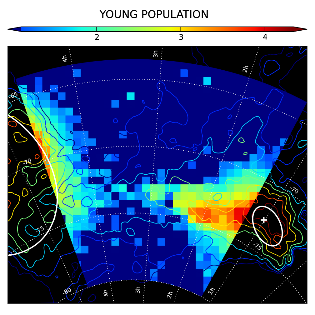
Figure 8.— A spatial density map of the Young Population stars in the Magellanic Bridge region, in a Hammer equal-area projection centered at $\alpha=3.3$ h and $\delta=-70$ deg. The color-coded value of each “pixel” is a logarithm of the number of stars per square degree area (as indicated on the color bar at the top of the figure), while each “pixel” area is $\sim 0.335\deg^{2}$. Note the fairly isolated “OGLE island” mid-way between the Clouds at $\alpha\approx 2.9$ h and $\delta\approx-73.5$ deg. A median background level was estimated from 40 most southern fields to be 1 star/deg² with a standard deviation of 6 stars/deg². Detections weaker than $2\sigma$ above the median background level have been given the background color. All number densities are listed in Table 2. An approximate location of the LMC disk and the main stellar body of the SMC are marked with white ellipses centered at $\alpha=05^{\rm h}29^{\rm m}$, $\delta=-69^{\circ}30^{\prime}$, and $\alpha=00^{\rm h}54^{\rm m}$, $\delta=-72^{\circ}57^{\prime}$, respectively. The white cross marks the SMC center of the outer SMC population found by Nidever et al. (2011) at $\alpha=01^{\rm h}00^{\rm m}31^{\rm s}$ and $\delta=-72^{\circ}43^{\prime}11^{\prime\prime}$. Color contours mark neutral hydrogen (Hi) emission integrated over the velocity range $80<v<400$ km/s, where each contour represents the Hi column density twice as large as the neighboring contour. Hi column densities are in the range $10^{20}-4\times 10^{21}{\rm cm}^{-2}$. Data were taken from the LAB survey of Galactic Hi (Kalberla et al., 2005).

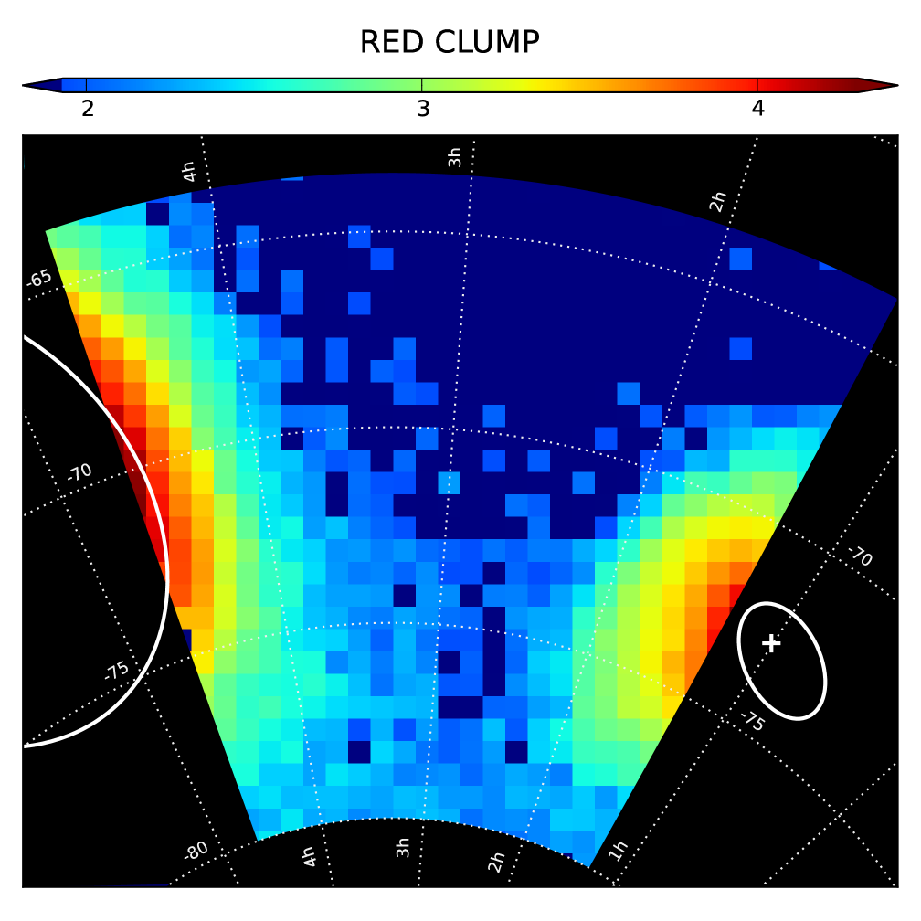
Figure 9.— Spatial density maps of the Red Clump stars in the Magellanic Bridge region, in a Hammer equal-area projection centered at $\alpha=3.3$ h and $\delta=-70$ deg. The color-coded value of each “pixel” is a logarithm of the number of stars per square degree area (as indicated on the color bar at the top of the figure), while each “pixel” area is $\sim 0.335\deg^{2}$. A median background level was estimated from 50 northern fields to be 36 stars/deg² with a standard deviation of 25 stars/deg². Detections weaker than $2\sigma$ above the median background level have been given the background color. All number densities are listed in Table 2. An approximate location of the LMC disk and the main stellar body of the SMC are marked with white ellipses centered at $\alpha=05^{\rm h}29^{\rm m}$, $\delta=-69^{\circ}30^{\prime}$, and $\alpha=00^{\rm h}54^{\rm m}$, $\delta=-72^{\circ}57^{\prime}$, respectively. The white cross marks the SMC center of the outer SMC population found by Nidever et al. (2011) at $\alpha=01^{\rm h}00^{\rm m}31^{\rm s}$ and $\delta=-72^{\circ}43^{\prime}11^{\prime\prime}$.

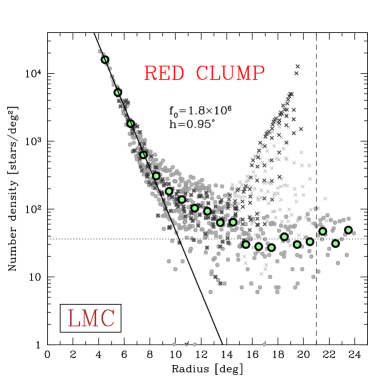
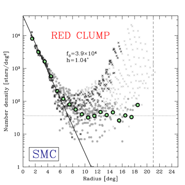
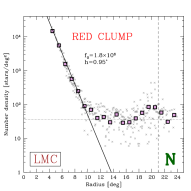
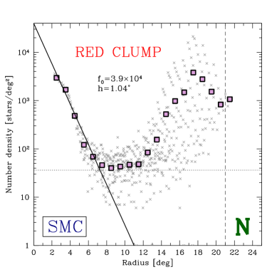
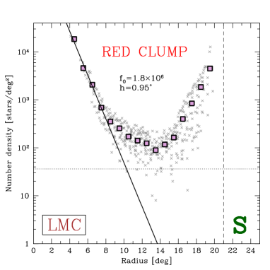
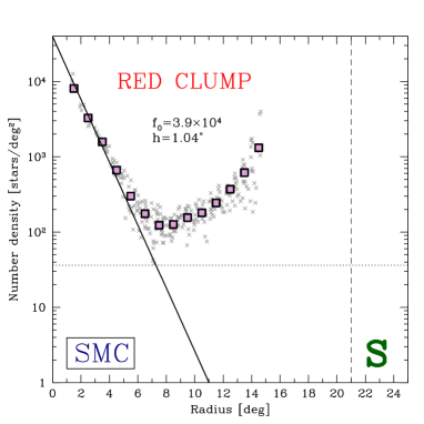
Figure 10.— Number densities of RC stars plotted against distance from the center of the LMC (left panels) and the SMC (right panels). Top panels show data for the entire density map, middle panels show data for the northern part and bottom panels for the southern part of the maps, respectively. The separation between north and south is with respect to the LMC center (left panels) and the SMC center (right panels). Light gray crosses represent all 754 subfields listed in Table 2 while black crosses represent subfields in the conservative MBR area between declinations $-70^{\circ}$ and $-75^{\circ}$. Dark gray dots show a subset of subfields excluding the SMC and its periphery (in the case of the LMC, i.e. left panels) or the LMC and its periphery (in the case of the SMC, i.e. right panels). Large green circles show median values of gray dots (top panels) while large purple squares show median values of gray crosses (middle and bottom panels). The solid line is a radial fit to dark gray dots in top panels for $r\leq 8^{\circ}$ in the form: $f=f_{0}\times e^{-r/h}$ where $f_{0}$ is the central density and $h$ is the scale height of the fit. Parameters of the fits are shown on each plot. The horizontal dotted line marks a median background value (36 stars/deg²) for RC stars based on 50 subfields in the northern part of the maps, where we do not expect LMC/SMC stars. The vertical dashed line at $r=21^{\circ}$ shows the approximate distance between the LMC and the SMC centers.

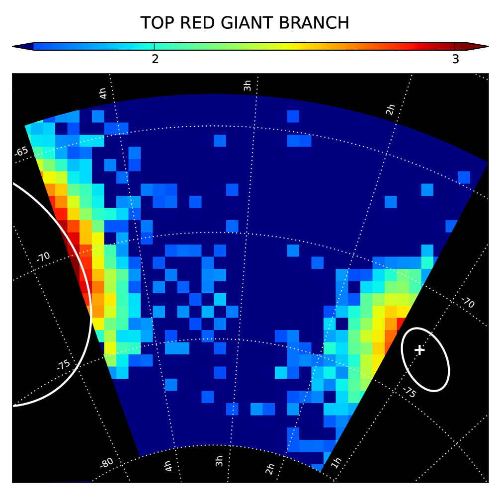
Figure 11.— Spatial density maps of the top part of the Red Giant Branch stars (I¡16 mag, V-I¡3 mag) in the Magellanic Bridge region, in a Hammer equal-area projection centered at $\alpha=3.3$ h and $\delta=-70$ deg. The color-coded value of each “pixel” is a logarithm of the number of stars per square degree area (as indicated on the color bar at the top of the figure), while each “pixel” area is $\sim 0.335\deg^{2}$. A median background level was estimated from 50 northern fields to be 16 stars/deg² with a standard deviation of 12 stars/deg². Detections weaker than $2\sigma$ above the median background level have been given the background color. All number densities are listed in Table 2. An approximate location of the LMC disk and the main stellar body of the SMC are marked with white ellipses centered at $\alpha=05^{\rm h}29^{\rm m}$, $\delta=-69^{\circ}30^{\prime}$, and $\alpha=00^{\rm h}54^{\rm m}$, $\delta=-72^{\circ}57^{\prime}$, respectively. The white cross marks the SMC center of the outer SMC population found by Nidever et al. (2011) at $\alpha=01^{\rm h}00^{\rm m}31^{\rm s}$ and $\delta=-72^{\circ}43^{\prime}11^{\prime\prime}$.

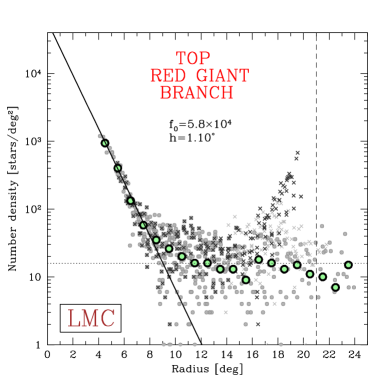
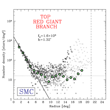
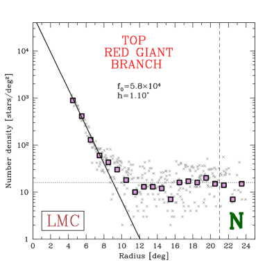
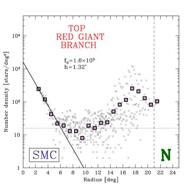
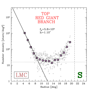
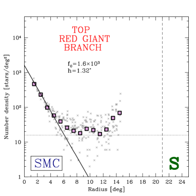
Figure 12.— Number densities of top RGB stars (I¡16 mag and V-I¡3 mag), plotted against distance from the center of the LMC (left panels) and the SMC (right panels). Top panels show data for the entire density map, middle panels show data for the northern part and bottom panels for the southern part of the maps, respectively. The separation between north and south is with respect to the LMC center (left panels) and the SMC center (right panels). Light gray crosses represent all 754 subfields listed in Table 2 while black crosses represent subfields in the conservative MBR area between declinations $-70^{\circ}$ and $-75^{\circ}$. Dark gray dots show a subset of subfields excluding the SMC and its periphery (in the case of the LMC, i.e. left panels) or the LMC and its periphery (in the case of the SMC, i.e. right panels). Large green circles show median values of gray dots (top panels) while large purple squares show median values of Grey crosses (middle and bottom panels). The solid line is a radial fit to dark gray dots in top panels for $r\leq 8^{\circ}$ in the form: $f=f_{0}\times e^{-r/h}$ where $f_{0}$ is the central density and $h$ is the scale height of the fit. Parameters of the fits are shown on each plot. The horizontal dotted line marks a median background value (12 stars/deg²) for top RGB stars based on 50 subfields in the northern part of the maps, where we do not expect LMC/SMC stars. The vertical dashed line at $r=21^{\circ}$ shows the approximate distance between the LMC and the SMC centers.

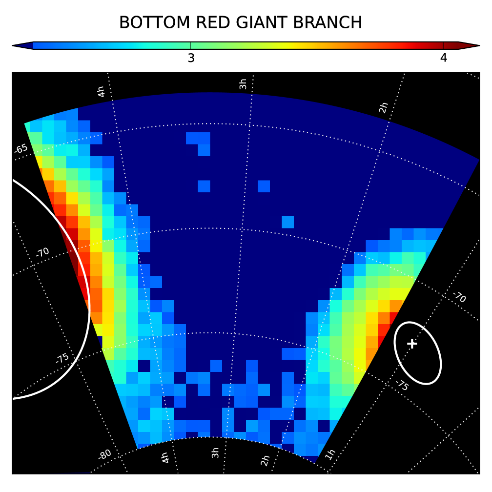
Figure 13.— Spatial density maps of the bottom part of the Red Giant Branch stars (I¿19 mag and I¡20 mag) in the Magellanic Bridge region, in a Hammer equal-area projection centered at $\alpha=3.3$ h and $\delta=-70$ deg. The color-coded value of each “pixel” is a logarithm of the number of stars per square degree area (as indicated on the color bar at the top of the figure), while each “pixel” area is $\sim 0.335\deg^{2}$. A median background level was estimated from 50 northern fields to be 112 stars/deg² with a standard deviation of 65 stars/deg². Detections weaker than $2\sigma$ above the median background level have been given the background color. All number densities are listed in Table 2. An approximate location of the LMC disk and the main stellar body of the SMC are marked with white ellipses centered at $\alpha=05^{\rm h}29^{\rm m}$, $\delta=-69^{\circ}30^{\prime}$, and $\alpha=00^{\rm h}54^{\rm m}$, $\delta=-72^{\circ}57^{\prime}$, respectively. The white cross marks the SMC center of the outer SMC population found by Nidever et al. (2011) at $\alpha=01^{\rm h}00^{\rm m}31^{\rm s}$ and $\delta=-72^{\circ}43^{\prime}11^{\prime\prime}$.

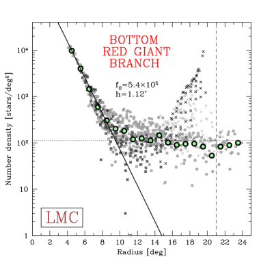
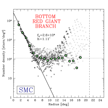
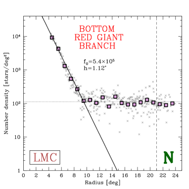
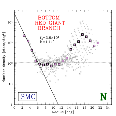
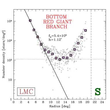
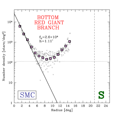
Figure 14.— Number densities of bottom RGB stars (I¡19 mag and I¿20 mag), plotted against distance from the center of the LMC (left panels) and the SMC (right panels). Top panels show data for the entire density map, middle panels show data for the northern part and bottom panels for the southern part of the maps, respectively. The separation between north and south is with respect to the LMC center (left panels) and the SMC center (right panels). Light gray crosses represent all 754 subfields listed in Table 2 while black crosses represent subfields in the conservative MBR area between declinations $-70^{\circ}$ and $-75^{\circ}$. Dark gray dots show a subset of subfields excluding the SMC and its periphery (in the case of the LMC, i.e. left panels) or the LMC and its periphery (in the case of the SMC, i.e. right panels). Large green circles show median values of gray dots (top panels) while large purple squares show median values of gray crosses (middle and bottom panels). The solid line is a radial fit to dark gray dots in top panels for $r\leq 8^{\circ}$ in the form: $f=f_{0}\times e^{-r/h}$ where $f_{0}$ is the central density and $h$ is the scale height of the fit. Parameters of the fits are shown on each plot. The horizontal dotted line marks a median background value (112 stars/deg²) for bottom RGB stars based on 50 subfields in the northern part of the maps, where we do not expect LMC/SMC stars. The vertical dashed line at $r=21^{\circ}$ shows the approximate distance between the LMC and the SMC centers.

References

- Bagheri et al. (2013) Bagheri, G., Cioni, M.-R. L., Napiwotzki, R. 2013, A&A, 551, 78
- Barger et al. (2013) Barger, K. A., Haffner, L. M., Bland-Hawthorn, J. 2013, ApJ, 771, 132
- Besla et al. (2007) Besla, G., Kallivayalil, N., Hernquist, L., Robertson, B., Cox, T. J., van der Marel, R. P., Alcock, C. 2007, ApJ, 668, 949
- Besla et al. (2012) Besla, G., Kallivayalil, N., Hernquist, L., van der Marel, R. P., Cox, T. J., Keres, D. 2012, MNRAS, 421, 2109
- Bica et al. (2008) Bica, E. L. D., Bonatto, C., Dutra, C. M., Santos, J. F. C., Jr. 2008, MNRAS, 389, 678
- Courtès et al. (1995) Courtès, G., Viton, M., Bowyer, S., Lampton, M., Sasseen, T. P., Wu, X.-Y. 1995, å, 297, 338
- Demers & Battinelli (1998) Demers, S., & Battinelli, P. 1998, AJ, 115, 154
- Diaz & Bekki (2012) Diaz, J. D., Bekki, K. 2012, ApJ, 750, 36
- Girardi et al. (2005) Girardi, L., Groenewegen, M. A. T., Hatziminaoglou, E., da Costa, L. 2005, A&A, 436, 895
- Grondin et al. (1992) Grondin, L., Demers, S., Kunkel, W. E. 1992, AJ, 103, 1234
- Harris (2007) Harris, J. 2007, ApJ, 658, 345
- Irwin et al. (1985) Irwin, M. J., Kunkel, W. E., Demers, S. 1985, Nature, 318, 160
- Irwin et al. (1990) Irwin, M. J., Demers, S., Kunkel, W. E. 1990, AJ, 99, 191
- Kalberla et al. (2005) Kalberla, P. M. W., Burton, W. B., Hartmann, D., Arnal, E. M., Bajaja, E., Morras, R., Poppel, W. G. L. 2005, å, 440, 775
- Kallivayalil et al. (2013) Kallivayalil, N., van der Marel, R. P., Besla, G., Anderson, J., Alcock, C. 2013, ApJ, 764, 161
- Kennicutt (1989) Kennicutt, R. C., Jr. 1989, ApJ, 344, 685
- Marcelin et al. (1985) Marcelin, M., Boulesteix, J., Georgelin, Y. 1985, Nature, 316, 705
- Mathewson & Ford (1984) Mathewson, D. S., Ford, V. L. 1984, IAUS, 108, 125
- Mathewson (1985) Mathewson, D. S. 1985, PASA, 6, 104
- Meaburn (1986) Meaburn, J. 1986, MNRAS, 223, 317
- Muller et al. (2003) Muller, E., Staveley-Smith, L., Zealey, W., Stanimirovic, S. 2003, MNRAS, 339, 105
- Muller et al. (2004) Muller, E., Stanimirovic, S., Rosolowsky, E., Staveley-Smith, L. 2004, ApJ, 616, 845
- Nidever et al. (2011) Nidever, D. L., Majewski, S. R., Munoz, R. R., Beaton, R. L., Patterson, R. J., Kunkel, W. E. 2011, ApJ, 733, 10
- Nidever et al. (2013) Nidever, D. L., Monachesi, A., Bell, E. F., Majewski, S. R., Munoz, R. R., Beaton, R. L. 2013, ApJ, 779, 145
- Nöel et al. (2013) Nöel, N. E. D., Conn, B. C., Carrera, R., Read, J. I., Rix, H.-W., Dolphin, A. 2013, ApJ, 768, 109
- Olsen et al. (2011) Olsen, K., Zaritsky, D., Blum, R. D., Boyer, M. L., Gordon, K. D. 2011, ApJ, 737, 29
- Putman (2000) Putman, M. E. 2000, PASA, 17, 1
- Ripepi et al. (2014) Ripepi, V., Cignoni, M., Tosi, M., Marconi, M., Musella, I., Grado, A., Limatola, L., Clementini, G. et al. 2014, MNRAS, 442, 1897
- Robin et al. (2003) Robin, A. C., Reyle, C., Derriere, S., Picaud, S. 2003, A&A, 409, 523
- Ruzicka et al. (2009) Ruzicka, A., Theis, C., Palous, J. 2009, ApJ, 691, 1807
- Schechter et al. (1993) Schechter, P. L., Mateo, M., Saha, A. 1993 PASP, 105, 1342
- Schlegel et al. (1998) Schlegel, D. J., Finkbeiner, D. P., & Davis, M. 1998, ApJ, 500, 525
- Shapley (1940) Shapley, H. 1940, Harvard Bulletin, 914, 8
- Sharma et al. (2011) Sharma, S., Bland-Hawthorn, J., Johnston, K. V., Binney, J. 2011, ApJ, 730, 3
- Szymański et al. (2011) Szymański, M. K., Udalski, A., Soszyński, I., Kubiak, M., Pietrzyński, G., Poleski, R., Wyrzykowski, Ł., Ulaczyk, K. 2011, Acta Astron., 61, 83
- Udalski et al. (1992) Udalski, A., Szymański, M. K., Kałużny, J., Kubiak, M., Mateo, M. 1992, Acta Astron., 42, 253
- Udalski (2003) Udalski, A. 2003, Acta Astron., 53, 291
- Udalski et al. (2008) Udalski, A., Szymański, M. K., Soszyński, I., Poleski, R. 2008, Acta Astron., 58, 69
- van der Marel (2001) van der Marel, R. P. 2001, AJ, 122, 1827
- Wozniak (2000) Woźniak, P. R. 2000, Acta Astron., 50, 421