Critical Behavior of the = 3, 4-Potts model on Quasiperiodic Decagonal Lattices
Abstract
In this study, we performed Monte Carlo simulations of the -Potts model on quasiperiodic decagonal lattices (QDL) to assess the critical behavior of these systems. Using the single histogram technique in conjunction with the finite-size scaling analysis, we estimate the infinite lattice critical temperatures and the leading critical exponents for and states. Our estimates for the critical exponents on QDL are in good agreement with the exact values on 2D periodic lattices, supporting the claim that both the and Potts model on quasiperiodic lattices belong to the same universality class as those on 2D periodic lattices.
pacs:
61.44.Br; 75.10.Hk; 05.10.LnI Introduction
Electron diffraction patterns exhibiting octagonal, decagonal, dodecagonal, and icosahedral point symmetry are found in various alloys. The most well-known pattern is the icosahedral phase in - alloys, which is observed when these materials are cooled at a rapid rate such that their constituent atoms do not have adequate time to form a crystal lattice. These structures are referred to as quasicrystals Shechtman (1984); Levine and Steinhardt (1986). In principle, quasicrystals are characterized as atomic structures that present long-range quasiperiodic translational and long-range orientational order. They can exhibit rotational symmetries otherwise forbidden to crystals. In the last decade, quasicrystals have attracted significant attention, mostly because of their stronger magnetic properties and enhanced elasticity at higher temperatures, compared with the traditional crystals.
A most intriguing research topic about quasicrystals is to determine whether its intrinsic complicated structure can result in a change of the universality class compared with its counterpart periodic structure. To this end, Potts model Potts (1952) offers a simple and feasible way to study quasicrystals from this perspective, as it contains both first- and second-order phase transitions. However, given the lack of periodicity of these quasiperiodic lattices, only numerical approaches can be performed. Previous Monte Carlo studies on the ferromagnetic Potts model for quasiperiodic lattices Wilson and Vause (1988, 1989); Ledue et al. (1997); Xiong et al. (1999); Fu et al. (2006); Bin et al. (2011) have revealed that both the systems belong to the same universality class, despite the critical temperature of the quasiperiodic lattices being higher than that of the square lattices. However, given the great variety of existing quasiperiodic lattices, this query has not been solved completely. Consequently, this necessitates extensive computational research for accurately estimating the static critical exponents in these lattices. To the best of our knowledge, studies concerning the Potts model on quasiperiodic lattices have been rarely reported in the literature.
The present study investigates the critical behavior of the ferromagnetic -Potts model on quasiperiodic decagonal lattices (QDL) to accurately estimate the infinite QDL critical temperature and critical exponents for each case. An interesting example of a natural structure which presents a decagonal symmetry is the quasicrystal found in the Khatyrka meteorite Bindi et al. (2015). The quasiperiodic lattices analyzed in this study were generated using the strip projection method Duneau and Katz (1985); Conway and Knowles (1986); Vogg and Ryder (1996) with spins placed in the vertices of the rhombi that constitute the QDL (Fig. 1). Periodic boundary conditions were applied on these lattices to avoid the boundary effects caused by the finite size.
This paper is organized as follows. Section II briefly describes the strip projection method adopted for generating the QDL and periodic boundary conditions used in the simulations. Details of the Potts model and Monte Carlo simulation approach are described in section III. In section IV, a succinct description of the finite-size scaling (FSS) relations used in the study is presented. In section V, we present the results for and Potts model and compare them with previous results on quasi-periodic lattices. In section VI, we conclude by summarizing the results and providing recommendations for further research.

II Strip Projection Method and Periodic Boundary Conditions
The strip projection method is a powerful technique for constructing periodic and non-periodic lattices. The methodology can be summarized as follows. First, starting from a regular lattice whose unit cell, , is spanned by the vectors , we can resolve into two mutually orthogonal subspaces, namely, and , of dimensions and , respectively, i.e., . Second, we define a “strip” as a set of all the points whose positions are obtained by adding any vector in to any vector in , i.e., . The required lattice, , is the projection in of all the points in that are included in the strip, i.e., . The requirement that any point lies in the strip is equivalent to the condition that the projection of in lies within the projection of in . This equivalence can be mathematically expressed as
| (1) |
where and , Accordingly, the lattice can be defined as follows:
| (2) |
One way to describe the projection of the points given by (where the ’s are integers) onto and is to choose an orthogonal basis in and an orthogonal basis in . Together they form a new basis of . Assuming , the relationship between the two basis can be given by a rigid rotational operation. By defining a rotation matrix , it is possible to determine the projection matrices using the following equations
| (3) |
where . The rotation matrix can be split into an submatrix and submatrix :
| (4) |
To generate the decagonal quasiperiodic lattice, the points in the finite region of a 5D hypercubic lattice () are projected onto an 2D subspace () only if these points are projected inside a rhombic icosahedron, which in this case is the “strip”. The resulting quasiperiodic lattice is obtained through the standard rotation matrix:
| (5) |
where and . The decagonal quasiperiodic lattice consists of two types of building blocks, usually represented by a fat rhombus with an acute angle of and a thin rhombus with an acute angle of , arranged according to specific matching rules. However, the quasiperiodic lattices are not suitable for Monte Carlo simulation with periodic boundary conditions. A more suitable approach is to construct a periodic approximation of these lattices. This can be realized by simply replacing the golden number in the sub-matrix of Eq. (5) by a rational number , where and are successive terms in the Fibonacci sequence
Fig. 1 shows the periodic approximation of the QDL inside a square projection window. The periodic boundary conditions are imposed at lattice sites closer to the square projection window. For finite lattices, the number of nearest neighbors at a given site range from to with a mean coordination number equal to . The mean coordination number is expected to be lower than , given the existence of a small fraction ( 1.0%) of sites on the boundary with a coordination number lower than in the finite lattices is analyzed in this study.
III Model and Monte Carlo Simulation
To study the critical behavior in the QDL, we updated our lattices using the Wolff algorithm Wolff (1989). For a fixed temperature, we define a Monte Carlo step (MCS) per spin by accumulating the flip times of all the spins and then dividing them by the total spin number. The Hamiltonian of the q-states ferromagnetic Potts model () can be written as
| (6) |
where is the Kronecker delta function, and the sum runs over all nearest neighbors of . We also define the order parameter as
| (7) |
where is the maximum number of spins in the same state and is the total number of spins. Once the critical region is established, we apply the single histogram method Ferrenberg and Landau (1991); Ferrenberg et al. (1995) along with FSS analysis to obtain accurate estimates of the critical temperature and critical exponents. System sizes up to are used in these simulations with MCS per spin performed at a single temperature , where configurations are discarded for thermalization. For each system size considered, we calculated the average of independent realizations to obtain reliable estimates of the statistical errors. The static thermodynamics quantities such as specific heat, magnetic susceptibility, logarithmic derivatives of the order parameter, and Binder’s fourth-order cumulants Binder (1981); Challa et al. (1986) are then calculated inside the critical region. Depending on the analysis of the location of the maximum values of these quantities and their magnitudes, one can estimate the infinite QDL critical temperature and critical exponents, respectively. For , we perform simulations at the temperatures and . The probability distribution obtained at each was reweighted from to for and from to for and . For , we perform simulations at the temperatures and . Here again, the probability distributions were reweighted from to for the first five smaller lattices and from to for the remaining lattices. The specific heat can be calculated from the fluctuations of the measurements
| (8) |
Similarly, from the fluctuations of , we can calculate the magnetic susceptibility
| (9) |
and the fourth-order magnetization cumulant
| (10) |
We can also calculate the logarithmic derivative of -power of , i.e,
| (11) | |||||
IV Finite-size scaling relations
IV.1 Potts Model
According to the finite-size scaling theory Fisher (1971); Fisher and Barber (1972), the free energy of a system of linear dimensional is described by the scaling ansatz
| (12) |
where ( is the infinite QDL critical temperature) and is the magnetic field. The leading critical exponents , , and define the universality class of the system. Considering zero-field regime, the derivatives of Eq. (12) yield important scaling equations, i.e.,
| (13) | |||||
| (14) | |||||
| (15) |
where , and are scaling functions, and is the temperature scaling variable. In addition, the critical temperature scales as
| (16) |
where is a constant and is the effective transition temperature for the QDL of linear size . This effective temperature can be obtained by the location of the peaks of the above quantities: , , and .
IV.2 Potts Model
Due to the presence in two-dimensional Potts model of a marginal operator Nauenberg and Scalapino (1980); J. L. Cardy and Scalapino (1980), which is absent in any other two-dimensional Potts model, the leading power-law scaling behavior of this model is modified by multiplicative logarithms. So Eqs. (12-16) must be modified to allow for these logarithmic corrections. The free energy scaling relation is suitably modified Aktekin (2001); Kenna (2004) by
| (17) |
where and . Moreover, considering zero-field regime, the derivatives of Eq.(17) yield suitable scaling equations for 4-state Potts model:
| (18) | |||||
| (19) | |||||
| (20) |
where , and are scaling functions, and is the temperature scaling variable. Correspondingly, the critical temperature scales as
| (21) |
In the above equations, the leading critical exponents Baxter (1982) for the Potts model on 2D periodic lattices are given by
V Results
V.1 Potts Model
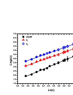
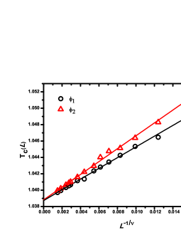
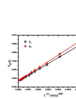
Taking the slope of the log-log plot of the maximum values of the quantities , and versus , three estimates are obtained for . Fig. 3 shows the log-log plot of these quantities for data simulated at . We obtained for , for , and for . By combining these results, we get . Similar analysis has been performed for , which yielded for , for and for . The effective range of is found to be by combining the above results. These estimates are in good agreement with the exact result based on the 2D periodic lattice (with ) and in reasonable agreement with the estimates that have previously been obtained for other quasiperiodic systems Ledue et al. (1997); Fu et al. (2006); Bin et al. (2011). After obtaining an estimate for , the infinite QDL critical temperature is computed by plotting the size dependence of the location of the peaks of and . Fig. 5 shows the finite-size scaling of the effective transition temperatures at . We obtained for and . With the simulations performed at the temperature , and using the corresponding estimated at this temperature, we obtained for and . These values of are higher than the exact value on the 2D periodic lattices Kihara et al. (1954), given by .
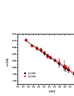
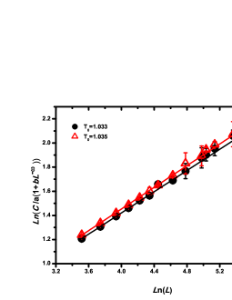
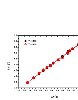
Using Eqs. (13-15) for the size dependence of the maximum values of , and , we can estimate , and , respectively. Fig. 5 shows the log-log plot of (measured at the temperature with maximum value of ) versus the linear size of the system . The slopes of the linear fit to the data obtained by simulating at and are and , respectively. Similarly, Fig. 7 shows the log-log plot of the maximum value of versus the linear size of the system. Particularly, in this plot, we have inserted correction-to-scaling terms L. N. Shchur and Butera (2008) to improve the fit quality of the data by scaling as
| (24) |
where the proper correlation amplitudes and and the nonuniversal correction-to-scaling exponent are chosen in order to minimize the of the fit. The slopes of the linear fit to the data obtained by simulating at and are and , respectively. Similarly, Fig. (7) shows a log-log plot of the maximum values of versus . The estimated values for at and are and , respectively. In these figures, the error bars are purely statistical and are estimated according to 100 different trial runs for each data point. The estimates of the ratios of the critical exponents and the average value for at each simulated temperature are summarized in Table 1. From Table 1, by multiplying the values of the ratios of the exponents at each simulated temperature by its respective value of , we obtain , and at , and , and at . On the 2D periodic lattice, the exact values for the Potts model of the critical exponents are , , and . The final estimates of the infinite QDL critical temperature and the critical exponents for the Potts model on QDL are summarized and compared with the exact values on the 2D periodic lattices in Table 3.
| 2D periodic lattice | ||||||
|---|---|---|---|---|---|---|
| 2D periodic lattice |
V.2 Potts Model
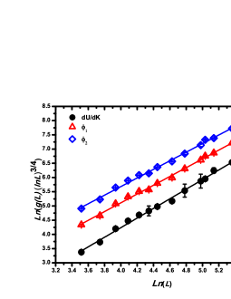
Fig. 3 shows the log-log plot of the size dependence of the maximum values of the quantities , and . Taking the slope of the quantities shown in Fig. 3, we obtain for , for and for . By combining these results, we find . Similarly at , we obtain for , for and for . Taking an average of the above results, we get . As one can see, these average values for are in reasonable agreement with the exact result on 2D periodic lattices, and especially for and , we have a very good convergence to this exact value.
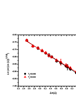
Fig. 9 shows the finite-size scaling of the effective transition temperatures. From Eq. (21) and locating the peaks of the quantities and , we find . Similar analysis has been done for the temperature with estimated at this temperature, which yielded . Following the case , these values are also higher than the exact value on 2D periodic lattices, given by .
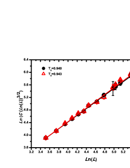
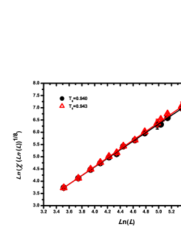
Using Eqs. (18-20) and taking the exact exponents from Eqs. 22 and 23 in the logarithmic-correction terms, we can estimate , and . Fig. 9 shows the log-log plot of (measured at the temperature with maximum value of ) versus linear size of the system. The slopes of the linear fit to the data obtained by simulating at and are and , respectively. Fig. 11 presents a log-log plot of the maximum values of versus . The slopes of the linear fit to the data obtained by simulating at and were and , respectively. Similarly, Fig. 11 shows the log-log plot of peaks of versus . Our estimates are at and at . The estimates of the ratios of the critical exponents and the average value for at each simulated temperature are summarized in Table 2.
From Table 2, by multiplying the values of the ratios of exponents at each simulated temperature by its respective value of , we obtain , and at , and , and at . The exact values of the critical exponents for the Potts model on 2D periodic lattice are , , and . The final estimates of the infinite QDL critical temperature and critical exponents for the Potts model on QDL are summarized and compared with the exact values on the 2D periodic lattices in Table 3.
VI Conclusions
We performed Monte Carlo simulations of the -Potts model on QDL to estimate the infinite critical temperature and the leading critical exponents for both and states. Our analysis reveals that for both and states, the infinite lattice critical temperature is higher than that of the square lattice, which can be attributed to the different geometric structure between the two models. For the Potts model, the leading critical exponents , and are, within the error precision, in good agreement with the corresponding values for the 2D periodic lattices, whereas for the Potts model, all the critical exponents are found to be very close to the exact values on the 2D periodic lattices. This provides strong evidence to support the claim that and Potts model on quasiperiodic lattices belong to the same universality class as those on 2D periodic lattices. Future work will involve numerical studies on 3D quasiperiodic lattices so that the icosahedral phase found in alloys such as -, - and - can also be better investigated.
Acknowledgements.
We wish to thank UFERSA for computational support and Prof. George Frederick T. da Silva for interesting discussions.References
- Shechtman (1984) D. Shechtman, Phys. Rev. Lett. 53, 1951 (1984).
- Levine and Steinhardt (1986) D. Levine and P. J. Steinhardt, Phys. Rev. B 34, 596 (1986).
- Potts (1952) R. B. Potts, Proc. Cambridge Philos. Soc. 48, 106 (1952).
- Wilson and Vause (1988) W. G. Wilson and C. A. Vause, Phys. Lett. A 126, 471 (1988).
- Wilson and Vause (1989) W. G. Wilson and C. A. Vause, Phys. Rev. B 39, 4651 (1989).
- Ledue et al. (1997) D. Ledue, T. Boutry, D. P. Landau, and J. Teillet, Phys. Rev. B 56, 10782 (1997).
- Xiong et al. (1999) G. Xiong, Z. H. Zhang, and D. C. Tian, Phys. A 265, 547 (1999).
- Fu et al. (2006) X. Fu, J. Ma, Z. Hou, and Y. Liu, Phys. Lett. A 351, 435 (2006).
- Bin et al. (2011) W. Z. Bin, H. Z. Lin, and F. X. Jun, Chin. Phys. Lett. 28, 046102 (2011).
- Bindi et al. (2015) L. Bindi, N. Yao, C. Lin, L. S. Hollister, C. L. Andronicos, V. V. Distler, M. P. Eddy, A. Kostin, V. Kryachko, G. J. MacPherson, et al., Natural quasicrystal with decagonal symmetry, Available from https://www.ncbi.nlm.nih.gov/pmc/articles/PMC4357871/ (2015), URL doi:10.1038/srep09111.
- Duneau and Katz (1985) M. Duneau and A. Katz, Phys. Rev. Lett. 54, 2688 (1985).
- Conway and Knowles (1986) J. H. Conway and K. M. Knowles, J. Phys. A19, 3645 (1986).
- Vogg and Ryder (1996) U. Vogg and P. L. Ryder, J. Non-Cryst. Sol. 194, 135 (1996).
- Wolff (1989) U. Wolff, Phys. Rev. Lett. 62, 361 (1989).
- Ferrenberg and Landau (1991) A. M. Ferrenberg and D. P. Landau, Phys. Rev. B 44, 5081 (1991).
- Ferrenberg et al. (1995) A. M. Ferrenberg, D. P. Landau, and R. H. Swendsen, Phys. Rev. E 51, 5092 (1995).
- Binder (1981) K. Binder, Z. Phys. 43, 119 (1981).
- Challa et al. (1986) M. S. S. Challa, D. P. Landau, and K. Binder, Phys. Lett. B 34, 1841 (1986).
- Fisher (1971) M. E. Fisher, Critical Phenomena (Academic, New York, 1971).
- Fisher and Barber (1972) M. E. Fisher and M. N. Barber, Phys. Rev. Lett. 28, 1516 (1972).
- Nauenberg and Scalapino (1980) M. Nauenberg and D. J. Scalapino, Phys. Rev. Lett. 44, 837 (1980).
- J. L. Cardy and Scalapino (1980) M. N. J. L. Cardy and D. J. Scalapino, Phys. Rev. B 22, 2560 (1980).
- Aktekin (2001) N. Aktekin, J. Stat. Phys. 104, 1397 (2001).
- Kenna (2004) R. Kenna, Nucl. Phys. B 691, 292 (2004).
- Baxter (1982) R. J. Baxter, Exact Solved Models in Statistical Mechanics (London: Academic Press Inc, 1982).
- Salas and Sokal (1997) J. Salas and A. D. Sokal, J. Stat. Phys. 88, 567 (1997).
- B. Berche and Shchur (2009) W. J. B. Berche, P. Butera and L. N. Shchur, Comp. Phys. Comput 180, 493 (2009).
- Kihara et al. (1954) T. Kihara, Y. Midzuno, and T. Shizume, J. Phys. Soc. Japan 9, 681 (1954).
- L. N. Shchur and Butera (2008) B. B. L. N. Shchur and P. Butera, Phys. Rev. B 77, 144410 (2008).