The CIB-lensing bispectrum: impact on primordial non-Gaussianity and detectability for the Planck mission

A. Curto1,2,3 M. Tucci4 M. Kunz4,5 E. Martínez-González1
1Instituto de Física de Cantabria, CSIC-Universidad de Cantabria, Avda. de los Castros s/n, 39005 Santander, Spain
2Astrophysics Group, Cavendish Laboratory, Madingley Road, Cambridge CB3 0H3, U.K.
3Kavli Institute for Cosmology Cambridge, Madingley Road, Cambridge, CB3 0HA, U.K.
4Département de Physique Théorique and Center for Astroparticle Physics, Université de Genève,  24 quai Ansermet, CH–1211 Genève 4, Switzerland
5African Institute for Mathematical Sciences, 6 Melrose Road, Muizenberg, 7945, South Africa
E-mail:curto@ifca.unican.es,acurto@mrao.cam.ac.uk
Abstract

We characterize the Cosmic Infrared Background (CIB)–lensing bispectrum which is one of the contributions to the three-point functions of Cosmic Microwave Background (CMB) maps in harmonic space. We show that the CIB–lensing bispectrum has a considerable strength and that it can be detected with high significance in the Planck high–frequency maps. We also present forecasts of the contamination on different shapes of the primordial non-Gaussianity fnlsubscript𝑓nlf_{\rm nl~{}}parameter produced by the CIB–lensing bispectrum and by the extragalactic point sources bispectrum in the Planck high–resolution CMB anisotropy maps. The local, equilateral and orthogonal shapes are considered for ’raw’ single–frequency (i.e., without applying any component separation technique) and foreground–reduced Planck temperature maps. The CIB–lensing correlation seems to mainly affect orthogonal shapes of the bispectrum – with Δfnl(ort)=21Δsuperscriptsubscript𝑓nlort21\Delta f_{\rm nl}^{\rm(ort)}=-21 and 8888-88 for the 143 and 217 GHz bands respectively – while point sources mostly impact equilateral shapes, with Δfnl(eq)=160,54Δsuperscriptsubscript𝑓nleq16054\Delta f_{\rm nl}^{\rm(eq)}=160,54 and 60 at 100, 143 and 217 GHz. However, the results indicate that these contaminants do not induce any relevant bias on Planck fnlsubscript𝑓nlf_{\rm nl~{}}estimates when foreground–reduced maps are considered: using SEVEM for the component separation we obtain Δfnl(ort)=10.5Δsuperscriptsubscript𝑓nlort10.5\Delta f_{\rm nl}^{\rm(ort)}=10.5 due to the CIB–lensing and Δfnl(eq)=30.4Δsuperscriptsubscript𝑓nleq30.4\Delta f_{\rm nl}^{\rm(eq)}=30.4 due to point sources, corresponding to 0.3σ0.3𝜎0.3\sigma and 0.45σ0.45𝜎0.45\sigma in terms of the Planck 2013 fnlsubscript𝑓nlf_{\rm nl} uncertainty. The component separation technique is, in fact, able to partially clean the extragalactic source contamination and the bias is reduced for all the shapes. We have further developed single- and multiple-frequency estimators based on the Komatsu, Spergel & Wandelt (2005) formalism that can be implemented to efficiently detect this signal.

keywords:
methods: data analysis – cosmic microwave background – extragalactic points sources – radio and far–IR: galaxies
pagerange: The CIB-lensing bispectrum: impact on primordial non-Gaussianity and detectability for the Planck missionLABEL:lastpagepubyear: 2014

1 Introduction

Primordial non–Gaussianity (NG) in the cosmic microwave background (CMB) radiation has emerged as one of the key tests for the physics of the early Universe, as different models of e.g. inflation predict slightly different deviations from Gaussian primordial fluctuations (see e.g. Bartolo et al., 2004; Bartolo et al., 2010; Yadav & Wandelt, 2010; Liguori et al., 2010; Martínez-González & Planck Collaboration, 2012). The latest constraints by the Planck111Planck (http://www.esa.int/Planck) is a project of the European Space Agency –ESA– with instruments provided by two scientific consortia funded by ESA member states with contributions from NASA. satellite put strong constraints on the amount of primordial NG that is present in the data (Planck 2013 results XXIV, 2014). But the precision of the Planck data requires great care concerning the subtraction of astrophysical contributions to the observed CMB anisotropies (so–called foregrounds). It is important to check all possible contributions for their expected level of contamination of the primordial NG estimate both on sky maps and on foreground-cleaned maps. At least the non-negligible foreground contributions should then be estimated jointly with the primordial ones, which requires the construction of an estimator also for the foregrounds.

Conventionally the CMB anisotropies ΔT(𝐧^)Δ𝑇^𝐧\Delta T(\hat{\mathbf{n}}), being a real-valued random field on the sky sphere, are expanded in spherical harmonics,

ΔT(𝐧^)=mamYm(𝐧^)Δ𝑇^𝐧subscript𝑚subscript𝑎𝑚subscript𝑌𝑚^𝐧\Delta T(\hat{\mathbf{n}})=\sum_{\ell m}a_{\ell m}Y_{\ell m}(\hat{\mathbf{n}}) (1)

and schematically we can write the coefficients amsubscript𝑎𝑚a_{\ell m} as a superposition of different contributions,

am=a~m(𝙲𝙼𝙱)+am(𝚏𝚐)+nm.subscript𝑎𝑚subscriptsuperscript~𝑎𝙲𝙼𝙱𝑚subscriptsuperscript𝑎𝚏𝚐𝑚subscript𝑛𝑚a_{\ell m}=\tilde{a}^{({\mathtt{CMB}})}_{\ell m}+a^{({\mathtt{fg}})}_{\ell m}+n_{\ell m}\,. (2)

Here the first term on the right hand side a~msubscript~𝑎𝑚\tilde{a}_{\ell m} is the primordial contribution, lensed by the intervening large–scale structure. The second term is the contribution due to foregrounds – in general there are both Galactic and extragalactic contributions, but in this paper we will neglect the former and use the term ‘foreground’ to denote the extragalactic contribution only. For the extragalactic foreground radiation we expect that radio sources dominate at low frequencies, and dusty star–forming galaxies creating the cosmic infrared background (CIB) at high frequencies. The final contribution is instrumental noise, obviously uncorrelated with the CMB and the foreground contributions, that we assume to be Gaussian.

The main tool to study primordial NG is the angular bispectrum, the three–point function of the amsubscript𝑎𝑚a_{\ell m},

a1m1a2m2a3m3=G123m1m2m3b123,delimited-⟨⟩subscript𝑎subscript1subscript𝑚1subscript𝑎subscript2subscript𝑚2subscript𝑎subscript3subscript𝑚3superscriptsubscript𝐺subscript1subscript2subscript3subscript𝑚1subscript𝑚2subscript𝑚3subscript𝑏subscript1subscript2subscript3\langle a_{\ell_{1}m_{1}}a_{\ell_{2}m_{2}}a_{\ell_{3}m_{3}}\rangle=G_{\ell_{1}\ell_{2}\ell_{3}}^{m_{1}m_{2}m_{3}}b_{\ell_{1}\ell_{2}\ell_{3}}\,, (3)

where the Gaunt integral (Komatsu & Spergel, 2001)

G123m1m2m3=d2𝐧^Y1m1(𝐧^)Y2m2(𝐧^)Y3m3(𝐧^)superscriptsubscript𝐺subscript1subscript2subscript3subscript𝑚1subscript𝑚2subscript𝑚3superscript𝑑2^𝐧subscript𝑌subscript1subscript𝑚1^𝐧subscript𝑌subscript2subscript𝑚2^𝐧subscript𝑌subscript3subscript𝑚3^𝐧G_{\ell_{1}\ell_{2}\ell_{3}}^{m_{1}m_{2}m_{3}}=\int d^{2}\hat{\mathbf{n}}Y_{\ell_{1}m_{1}}(\hat{\mathbf{n}})Y_{\ell_{2}m_{2}}(\hat{\mathbf{n}})Y_{\ell_{3}m_{3}}(\hat{\mathbf{n}}) (4)

takes care of rotational symmetry, and where the non-trivial contribution to the three-point function is encoded in the reduced bispectrum b123subscript𝑏subscript1subscript2subscript3b_{\ell_{1}\ell_{2}\ell_{3}}.

The product of three amsubscript𝑎𝑚a_{\ell m} as written in Eq. (2) will not only contain a primordial contribution. In addition there are additional elements that involve non-primordial terms, some of them already studied in previous works, such as the ‘foreground’ contribution given schematically by am(𝚏𝚐)3delimited-⟨⟩subscriptsuperscript𝑎𝚏𝚐3𝑚\langle a^{{({\mathtt{fg}})}3}_{\ell m}\rangle (see e.g. Lacasa et al., 2014; Pénin et al., 2013), a contribution from the correlation between the lensing of the CMB and the integrated Sachs–Wolfe (ISW) effect contained in the a~m(𝙲𝙼𝙱)3delimited-⟨⟩subscriptsuperscript~𝑎𝙲𝙼𝙱3𝑚\langle\tilde{a}^{({\mathtt{CMB}})3}_{\ell m}\rangle term (see e.g. Mangilli et al., 2013) and finally a contribution from the correlation between the lensing of the CMB and extragalactic foregrounds. This article is focusing on the last correlation, already detected with a significance of 42σ𝜎\sigma by Planck 2013 results XVIII (2014) considering statistical errors only (19σ𝜎\sigma when systematics are included). The CIB–lensing correlation arises as the large–scale structure (LSS) both lenses the CMB and emits the ‘foreground’ (radio or CIB) radiation. The main contribution here is expected due to the CIB–lensing correlation, as in radio galaxies the clustering signal is highly diluted by the broadness of their luminosity function and of their redshift distribution (e.g., Toffolatti et al., 2005).

In this paper we focus on the CIB–lensing bispectrum, for two reasons. Firstly, in order to ensure that the CMB constraints on primordial NG are accurate, we need to check that the additional contributions are under control. In Planck 2013 results XXIV (2014) the ISW–lensing contribution was fit simultaneously with the primordial contribution, and was shown to be small. Lacasa et al. (2012) and Curto et al. (2013) studied the bispectrum of unresolved point sources and concluded that it is small enough to neglect. However, the situation of the CIB–lensing contribution was so far not investigated in detail, and this paper aims to close this gap. Secondly, probing the non–Gaussianity due to the large–scale structure is not only important for assessing the contamination of the primordial NG, but is also interesting in its own right. The LSS contains important information on the late–time evolution and content of the universe, as well as on the formation and evolution of galaxies. Studying the CIB–lensing correlation is thus not only important to assess the reliability of the constraints on primordial fnlsubscript𝑓nlf_{\rm nl}, but also potentially useful for cosmology and astrophysics.

The outline of the paper is as follows: in Section 2 we discuss the CIB–lensing contribution as well as the CIB model that we will use. In Section 3 we estimate the bias on fnlsubscript𝑓nlf_{\rm nl~{}}for local, equilateral and orthogonal configurations. We perform the calculation both for raw frequency maps and for linear combinations of maps that remove most of the astrophysical foregrounds, following the SEVEM component separation method used by the Planck collaboration (see, e.g. Planck 2013 results XII, 2014). We then construct in Sections 4 and 5 an optimal estimator for measuring the CIB–lensing bispectrum and assess the level at which we expect to be able to detect it with Planck data before presenting our conclusions in Section 6. In the four attached appendices we provide more details on our model of CIB anisotropies power spectra (including a new parameter fit of the Planck measurement of CIB power spectra) and on the calculation of power spectra and bispectra.

2 Modelling the CIB and CIB–lensing power spectra
Refer to caption
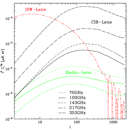
Figure 1: Predicted power spectra of the lensing correlation with ISW (red curve), CIB (black curves) and radio sources (green curves) at the Planck frequencies relevant for cosmological analysis.
Refer to caption
Refer to caption
Refer to caption
Refer to caption
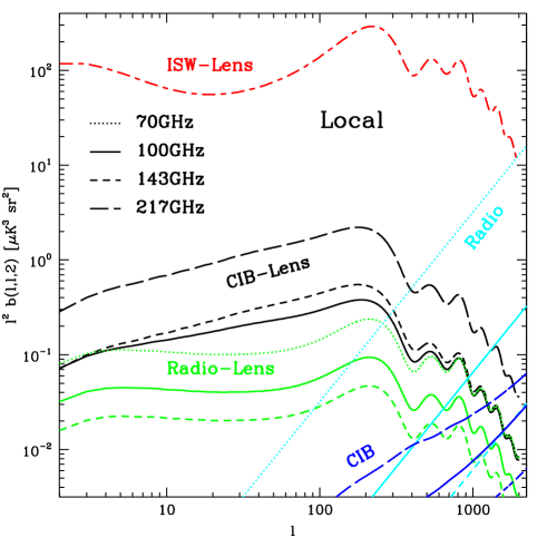
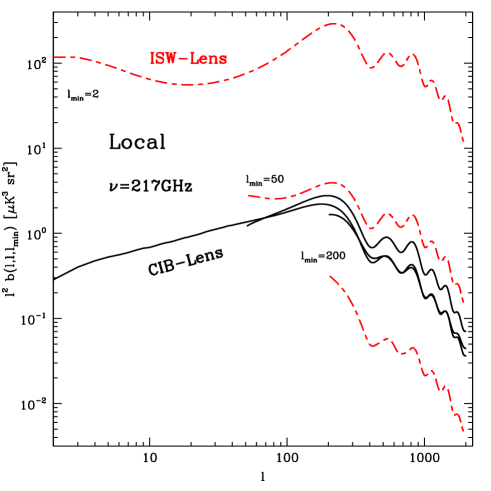
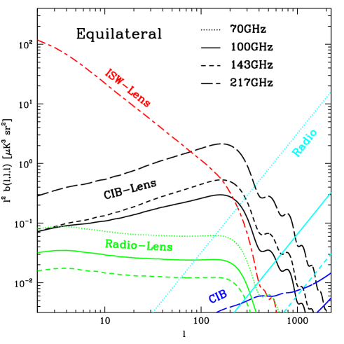
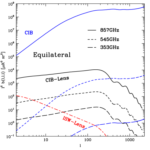
Figure 2: Predicted bispectra for the local (upper panels) and equilateral (1=2=3subscript1subscript2subscript3\ell_{1}=\ell_{2}=\ell_{3}; lower panels) configurations. Contributions are as in Figure 1, plus bispectra from radio sources (cyan curves) and IR galaxies (blue curves). Frequencies are indicated inside the plots. In the upper left panel, “local” bispectra are plotted at different frequencies (from 70 to 217 GHz) and for 1=2subscript1subscript2\ell_{1}=\ell_{2} and 3=min=2subscript3subscriptmin2\ell_{3}=\ell_{\rm min}=2; in the upper right panel, they are plotted at 217 GHz for 3=min=2,50,200formulae-sequencesubscript3subscriptmin250200\ell_{3}=\ell_{\rm min}=2,~{}50,~{}200.

The interplay between the CMB gravitational lensing and CIB intensity fluctuations are studied in this work in terms of the cross-bispectrum (the so called CIB–lensing bispectrum), its detectability levels and the bias on the primordial non-Gaussianity through the fnlsubscript𝑓nlf_{\rm nl~{}}parameter. The observed temperature fluctuations, neglecting other foreground sources, can be expanded at first order as (see e.g. Goldberg & Spergel, 1999; Hu, 2000):

ΔT(𝐧^)=ΔT𝙲𝙼𝙱(𝐧^+ϕ(𝐧^))+ΔT𝙲𝙸𝙱(𝐧^)ΔT𝙲𝙼𝙱(𝐧^)+(ΔT𝙲𝙼𝙱(𝐧^))ϕ(𝐧^)+ΔT𝙲𝙸𝙱(𝐧^),Δ𝑇^𝐧Δsubscript𝑇𝙲𝙼𝙱^𝐧italic-ϕ^𝐧Δsubscript𝑇𝙲𝙸𝙱^𝐧similar-to-or-equalsΔsubscript𝑇𝙲𝙼𝙱^𝐧Δsubscript𝑇𝙲𝙼𝙱^𝐧italic-ϕ^𝐧Δsubscript𝑇𝙲𝙸𝙱^𝐧\Delta T(\hat{\mathbf{n}})=\Delta T_{{\mathtt{CMB}}}(\hat{\mathbf{n}}+\nabla\phi(\hat{\mathbf{n}}))+\Delta T_{{{\mathtt{CIB}}}}(\hat{\mathbf{n}})\simeq\Delta T_{{\mathtt{CMB}}}(\hat{\mathbf{n}})+\nabla\big{(}\Delta T_{{\mathtt{CMB}}}(\hat{\mathbf{n}})\big{)}\nabla\phi(\hat{\mathbf{n}})+\Delta T_{{\mathtt{CIB}}}(\hat{\mathbf{n}})\,, (5)

where ϕ(𝐧^)italic-ϕ^𝐧\phi(\hat{\mathbf{n}}) is the lensing potential, ΔT𝙲𝙼𝙱(𝐧^)Δsubscript𝑇𝙲𝙼𝙱^𝐧\Delta T_{{\mathtt{CMB}}}(\hat{\mathbf{n}}) are the primordial CMB anisotropies and ΔT𝙲𝙸𝙱(𝐧^)Δsubscript𝑇𝙲𝙸𝙱^𝐧\Delta T_{{\mathtt{CIB}}}(\hat{\mathbf{n}}) are the anisotropies due to the CIB. Going into the spherical harmonic space, the observed anisotropies are:

am=a~m(𝙲𝙼𝙱)+am(𝙲𝙸𝙱)=am(𝙲𝙼𝙱)+m′′m′′(1)mG′′mmm′′[(+1)(+1)+′′(′′+1)2am(𝙲𝙼𝙱)ϕ′′m′′]+am(𝙲𝙸𝙱),subscript𝑎𝑚subscriptsuperscript~𝑎𝙲𝙼𝙱𝑚subscriptsuperscript𝑎𝙲𝙸𝙱𝑚subscriptsuperscript𝑎𝙲𝙼𝙱𝑚subscriptsuperscriptsuperscript𝑚superscript′′superscript𝑚′′superscript1𝑚superscriptsubscript𝐺superscriptsuperscript′′𝑚superscript𝑚superscript𝑚′′delimited-[]superscriptsuperscript11superscript′′superscript′′12subscriptsuperscript𝑎𝙲𝙼𝙱superscriptsuperscript𝑚subscriptitalic-ϕsuperscript′′superscript𝑚′′subscriptsuperscript𝑎𝙲𝙸𝙱𝑚a_{\ell m}=\tilde{a}^{({\mathtt{CMB}})}_{\ell m}+a^{({\mathtt{CIB}})}_{\ell m}=a^{({\mathtt{CMB}})}_{\ell m}+\sum_{\ell^{\prime}m^{\prime}\ell^{\prime\prime}m^{\prime\prime}}(-1)^{m}G_{\ell\ell^{\prime}\ell^{\prime\prime}}^{mm^{\prime}m^{\prime\prime}}\Big{[}\frac{\ell^{\prime}(\ell^{\prime}+1)-\ell(\ell+1)+\ell^{\prime\prime}(\ell^{\prime\prime}+1)}{2}a^{({\mathtt{CMB}})}_{\ell^{\prime}m^{\prime}}\phi_{\ell^{\prime\prime}m^{\prime\prime}}\Big{]}+a^{({\mathtt{CIB}})}_{\ell m}, (6)

where a~m(𝙲𝙼𝙱)subscriptsuperscript~𝑎𝙲𝙼𝙱𝑚\tilde{a}^{({\mathtt{CMB}})}_{\ell m}, am(𝙲𝙼𝙱)subscriptsuperscript𝑎𝙲𝙼𝙱𝑚a^{({\mathtt{CMB}})}_{\ell m}, am(𝙲𝙸𝙱)subscriptsuperscript𝑎𝙲𝙸𝙱𝑚a^{({\mathtt{CIB}})}_{\ell m} and ϕmsubscriptitalic-ϕ𝑚\phi_{\ell m} are the spherical harmonic coefficients of the observed/primordial CMB, CIB and gravitational potential anisotropies, respectively, and G′′mmm′′superscriptsubscript𝐺superscriptsuperscript′′𝑚superscript𝑚superscript𝑚′′G_{\ell\ell^{\prime}\ell^{\prime\prime}}^{mm^{\prime}m^{\prime\prime}} is the Gaunt coefficient (see Eq. 4).

The angular power spectra of CIB fluctuations and of their cross–correlation with the CMB lensing are typically written in the Limber approximation as (e.g., Song et al., 2003, see also Appendix A for a full derivation):

C(𝙲𝙸𝙱)(ν,ν)=am(𝙲𝙸𝙱)am(𝙲𝙸𝙱)superscriptsubscript𝐶𝙲𝙸𝙱𝜈superscript𝜈delimited-⟨⟩subscriptsuperscript𝑎𝙲𝙸𝙱𝑚subscriptsuperscript𝑎𝙲𝙸𝙱𝑚\displaystyle C_{\ell}^{({\mathtt{CIB}})}(\nu,\nu^{\prime})=\langle a^{({\mathtt{CIB}})*}_{\ell m}a^{({\mathtt{CIB}})}_{\ell m}\rangle =\displaystyle= 0χdχχ2Wν(𝙲𝙸𝙱)(χ)Wν(𝙲𝙸𝙱)(χ)Pgg(k=/χ,χ);superscriptsubscript0subscript𝜒𝑑𝜒superscript𝜒2superscriptsubscript𝑊𝜈𝙲𝙸𝙱𝜒superscriptsubscript𝑊superscript𝜈𝙲𝙸𝙱𝜒subscript𝑃gg𝑘𝜒𝜒\displaystyle\int_{0}^{\chi_{*}}{d\chi\over\chi^{2}}\,W_{\nu}^{({\mathtt{CIB}})}(\chi)W_{\nu^{\prime}}^{({\mathtt{CIB}})}(\chi)\,P_{\rm gg}(k=\ell/\chi,\chi)\,;
C(𝙲𝙸𝙱𝙻𝚎𝚗𝚜)(ν)=ϕmam(𝙲𝙸𝙱)superscriptsubscript𝐶𝙲𝙸𝙱𝙻𝚎𝚗𝚜𝜈delimited-⟨⟩subscriptsuperscriptitalic-ϕ𝑚subscriptsuperscript𝑎𝙲𝙸𝙱𝑚\displaystyle C_{\ell}^{({\mathtt{CIB-Lens}})}(\nu)=\langle\phi^{*}_{\ell m}a^{({\mathtt{CIB}})}_{\ell m}\rangle =\displaystyle= 0χdχχ2Wν(𝙲𝙸𝙱)(χ)W(𝙻𝚎𝚗𝚜)(k,χ)Pδg(k=/χ,χ).superscriptsubscript0subscript𝜒𝑑𝜒superscript𝜒2superscriptsubscript𝑊𝜈𝙲𝙸𝙱𝜒superscript𝑊𝙻𝚎𝚗𝚜𝑘𝜒subscript𝑃𝛿g𝑘𝜒𝜒\displaystyle\int_{0}^{\chi_{*}}{d\chi\over\chi^{2}}\,W_{\nu}^{({\mathtt{CIB}})}(\chi)W^{({\mathtt{Lens}})}(k,\chi)\,P_{\delta{\rm g}}(k=\ell/\chi,\chi)\,. (7)

The integral is over the comoving distance χ𝜒\chi along the line of sight, and extends up to the comoving distance of the last scattering surface χ=χ𝜒subscript𝜒\chi=\chi_{*} (in practice the integral is computed up to redshift 7 because of the negligible contribution of CIB fluctuations at higher redshifts). The W(𝙲𝙸𝙱)(χ)superscript𝑊𝙲𝙸𝙱𝜒W^{({\mathtt{CIB}})}(\chi) and W(𝙻𝚎𝚗𝚜)(k,χ)superscript𝑊𝙻𝚎𝚗𝚜𝑘𝜒W^{({\mathtt{Lens}})}(k,\chi) functions are the redshift weights for CIB fluctuations and for the lensing potential ϕitalic-ϕ\phi, respectively,

Wν(𝙲𝙸𝙱)(χ)=a(χ)j¯ν(χ)W(𝙻𝚎𝚗𝚜)(k,χ)=3Ωma(χ)(H0ck)2χχχχ,formulae-sequencesuperscriptsubscript𝑊𝜈𝙲𝙸𝙱𝜒𝑎𝜒subscript¯𝑗𝜈𝜒superscript𝑊𝙻𝚎𝚗𝚜𝑘𝜒3subscriptΩ𝑚𝑎𝜒superscriptsubscript𝐻0𝑐𝑘2subscript𝜒𝜒subscript𝜒𝜒W_{\nu}^{({\mathtt{CIB}})}(\chi)=a(\chi)\,\bar{j}_{\nu}(\chi)~{}~{}~{}~{}~{}~{}~{}~{}~{}~{}~{}~{}W^{({\mathtt{Lens}})}(k,\chi)=3{\Omega_{m}\over a(\chi)}\bigg{(}{H_{0}\over ck}\bigg{)}^{2}{\chi_{*}-\chi\over\chi_{*}\chi}\,, (8)

where a(χ)𝑎𝜒a(\chi) is the scale factor and j¯ν(χ)subscript¯𝑗𝜈𝜒\bar{j}_{\nu}(\chi) is the mean CIB emissivity at frequency ν𝜈\nu as a function of χ𝜒\chi:

j¯ν(χ)=(1+z)(dχdz)10ScSd2NdSdz𝑑S.subscript¯𝑗𝜈𝜒1𝑧superscript𝑑𝜒𝑑𝑧1superscriptsubscript0subscript𝑆𝑐𝑆superscript𝑑2𝑁𝑑𝑆𝑑𝑧differential-d𝑆\bar{j}_{\nu}(\chi)=(1+z)\bigg{(}{d\chi\over dz}\bigg{)}^{-1}\int_{0}^{S_{c}}\,S{d^{2}N\over dSdz}dS\,. (9)

Here d2N/dSdzsuperscript𝑑2𝑁𝑑𝑆𝑑𝑧d^{2}N/dSdz denotes galaxies number counts per interval of flux density and redshift, and Scsubscript𝑆𝑐S_{c} is the flux limit above which sources are subtracted or masked222Hereafter, we use as flux limit for the Planck mission the 90% completeness level of the Planck Catalogue of Compact Sources, given in Planck 2013 results XXVIII (2014).. We compute the redshift evolution of the CIB emissivity from the model of galaxy evolution of Béthermin et al. (2011)333We use number counts of the so–called mean model, see the http://www.ias.u-psud.fr/irgalaxies/ web page.. This is a backward evolution model based on parametric luminosity functions for two populations of galaxies: normal and starburst galaxies. It uses spectral energy distribution templates for the two galaxy populations taken from the Lagache et al. (2004) library. The model is described by 13 free parameters and the best–fit values are computed using observational number counts and luminosity functions from mid–infrared to millimetre wavelengths (Béthermin et al., 2011). This CIB model was previously used by Pénin et al. (2012) before and then applied to Planck results (Planck early results XVIII, 2011; Planck 2013 results XXX, 2014) in order to compute CIB and CIB–lensing power spectra.

In Eq. (7), Pgg(k,χ)subscript𝑃gg𝑘𝜒P_{\rm gg}(k,\chi) and Pδg(k,χ)subscript𝑃𝛿g𝑘𝜒P_{\delta{\rm g}}(k,\chi) are respectively the 3D power spectrum of galaxies and of the cross–correlation between galaxies and the dark matter (DM) density field. In the context of the halo model (Scherrer & Bertschinger, 1991; Seljak, 2000; Scoccimarro et al., 2001; Cooray & Sheth, 2002), the power spectra are the sum of the contribution of the clustering in one single halo (1–halo term) and in two different halos (2–halo term):

Pgg(k)=Pgg1h(k)+Pgg2h(k)subscript𝑃gg𝑘superscriptsubscript𝑃gg1𝑘superscriptsubscript𝑃gg2𝑘\displaystyle P_{\rm gg}(k)=P_{\rm gg}^{1h}(k)+P_{\rm gg}^{2h}(k) Pδg(k)=Pδg1h(k)+Pδg2h(k)subscript𝑃𝛿g𝑘superscriptsubscript𝑃𝛿g1𝑘superscriptsubscript𝑃𝛿g2𝑘\displaystyle P_{\delta{\rm g}}(k)=P_{\delta{\rm g}}^{1h}(k)+P_{\delta{\rm g}}^{2h}(k)
Pgg1h(k)=𝑑Mn(M)Ngal(Ngal1)n¯gal2u2(k,M)superscriptsubscript𝑃gg1𝑘differential-d𝑀𝑛𝑀delimited-⟨⟩subscript𝑁galsubscript𝑁gal1subscriptsuperscript¯𝑛2galsuperscript𝑢2𝑘𝑀\displaystyle P_{\rm gg}^{1h}(k)=\int\,dM\,n(M){\langle N_{\rm gal}(N_{\rm gal}-1)\rangle\over\bar{n}^{2}_{\rm gal}}u^{2}(k,M) Pδg1h(k)=𝑑Mn(M)Mρ¯Ngaln¯galu2(k,M)superscriptsubscript𝑃𝛿g1𝑘differential-d𝑀𝑛𝑀𝑀¯𝜌delimited-⟨⟩subscript𝑁galsubscript¯𝑛galsuperscript𝑢2𝑘𝑀\displaystyle P_{\delta{\rm g}}^{1h}(k)=\int\,dM\,n(M){M\over\bar{\rho}}{\langle N_{\rm gal}\rangle\over\bar{n}_{\rm gal}}u^{2}(k,M)
Pgg2h(k)=Plin(k)[𝑑Mn(M)b(M)Ngaln¯galu(k,M)]2superscriptsubscript𝑃gg2𝑘subscript𝑃lin𝑘superscriptdelimited-[]differential-d𝑀𝑛𝑀𝑏𝑀delimited-⟨⟩subscript𝑁galsubscript¯𝑛gal𝑢𝑘𝑀2\displaystyle P_{\rm gg}^{2h}(k)=P_{\rm lin}(k)\bigg{[}\int\,dM\,n(M)b(M){\langle N_{\rm gal}\rangle\over\bar{n}_{\rm gal}}u(k,M)\bigg{]}^{2} Pδg2h(k)=Plin(k)dM1n(M1)b(M1)M1ρ¯u(k,M)×\displaystyle P_{\delta{\rm g}}^{2h}(k)=P_{\rm lin}(k)\,\int\,dM_{1}\,n(M_{1})b(M_{1}){M_{1}\over\bar{\rho}}u(k,M)\,\times (10)
×dM2n(M2)b(M2)Ngaln¯galu(k,M2)\displaystyle~{}~{}~{}~{}~{}~{}~{}~{}~{}~{}~{}~{}~{}~{}~{}~{}~{}~{}\times\int\,dM_{2}\,n(M_{2})b(M_{2}){\langle N_{\rm gal}\rangle\over\bar{n}_{\rm gal}}u(k,M_{2})

The main inputs required for the calculations of Pgg(k)subscript𝑃gg𝑘P_{\rm gg}(k) and Pδg(k)subscript𝑃𝛿g𝑘P_{\delta{\rm g}}(k) are: (i) the mass function n(M)𝑛𝑀n(M) of DM halos –we use the mass function fit of Tinker et al. (2008) with its associated prescription for the halo bias, b(M)𝑏𝑀b(M) (see Tinker et al., 2010)–; (ii) the distribution of DM within halos, u(k,M)𝑢𝑘𝑀u(k,M), –we use the NFW (Navarro et al., 1997) profile–; and (iii) the Halo Occupation Distribution (HOD), that is a statistical description of how DM halos are populated with galaxies. We model the HOD using a central-satellite formalism (e.g., Kravtsov et al., 2004; Zheng et al., 2005): it introduces a distinction between central galaxies, which lies at the centre of the halo, and satellite galaxies that populate the rest of the halo and are distributed in proportion to the halo mass profile. The mean number of galaxies in a halo of mass M𝑀M is thus written as Ngal=Ncen+Nsatdelimited-⟨⟩subscript𝑁galdelimited-⟨⟩subscript𝑁cendelimited-⟨⟩subscript𝑁sat\langle N_{{\rm gal}}\rangle=\langle N_{\rm cen}\rangle+\langle N_{\rm sat}\rangle. Following Tinker & Wetzel (2010), the mean occupation functions of central and satellite galaxies are:

Ncen=12[1+erf(logMlogMminσlogM)],delimited-⟨⟩subscript𝑁cen12delimited-[]1erf𝑀subscript𝑀minsubscript𝜎𝑀\langle N_{\rm cen}\rangle={1\over 2}\Bigg{[}1+{\rm erf}\Bigg{(}{\log M-\log M_{\rm min}\over\sigma_{\log M}}\Bigg{)}\Bigg{]}\,, (11)

and

Nsat=12[1+erf(logMlog2MminσlogM)](MMsat)αsat,delimited-⟨⟩subscript𝑁sat12delimited-[]1erf𝑀2subscript𝑀minsubscript𝜎𝑀superscript𝑀subscript𝑀satsubscript𝛼sat\langle N_{\rm sat}\rangle={1\over 2}\Bigg{[}1+{\rm erf}\Bigg{(}{\log M-\log 2M_{\rm min}\over\sigma_{\log M}}\Bigg{)}\Bigg{]}\Bigg{(}{M\over M_{\rm sat}}\Bigg{)}^{\alpha_{\rm sat}}\,, (12)

where Mminsubscript𝑀minM_{\rm min}, αsatsubscript𝛼sat\alpha_{\rm sat}, Msatsubscript𝑀satM_{\rm sat} and σlogMsubscript𝜎𝑀\sigma_{\log M} are free parameters. Within this parametrisation, most of the halos with MMmingreater-than-or-similar-to𝑀subscript𝑀minM\ga M_{\rm min} contain a central galaxy. For satellite galaxies the mass threshold is chosen to be twice Mminsubscript𝑀minM_{\rm min}, so that halos with a low probability of having a central galaxy are unlikely to contain a satellite galaxy. The number of satellite galaxies grows with a slope αsatsubscript𝛼sat\alpha_{\rm sat} for high–mass halos. Moreover, assuming a Poisson distribution for Nsatsubscript𝑁satN_{\rm sat}, we can write Ngal(Ngal1)=2Nsat+Nsat2delimited-⟨⟩subscript𝑁galsubscript𝑁gal12delimited-⟨⟩subscript𝑁satsuperscriptdelimited-⟨⟩subscript𝑁sat2\langle N_{\rm gal}(N_{\rm gal}-1)\rangle=2\langle N_{\rm sat}\rangle+\langle N_{\rm sat}\rangle^{2} (Zheng et al., 2005). Finally, in Eq. (10), ρ¯¯𝜌\bar{\rho} is the background density, n¯galsubscript¯𝑛gal\bar{n}_{\rm gal} is the mean number of galaxies given by 𝑑Mn(M)Ngaldifferential-d𝑀𝑛𝑀delimited-⟨⟩subscript𝑁gal\int dMn(M)\langle N_{\rm gal}\rangle, and Plinsubscript𝑃linP_{\rm lin} is the linear DM power spectrum.

Following the analysis in Planck early results XVIII (2011), we restrict the free HOD parameters to only Mminsubscript𝑀minM_{\rm min} and αsatsubscript𝛼sat\alpha_{\rm sat} by imposing Msat=3.3Mminsubscript𝑀sat3.3subscript𝑀minM_{\rm sat}=3.3M_{\rm min} and σlogM=0.65subscript𝜎𝑀0.65\sigma_{\log M}=0.65. Moreover, because of the uncertainty of the evolution model of galaxies at high redshift, the effective mean emissivity jeffsubscript𝑗effj_{\rm eff} at z>3.5𝑧3.5z>3.5 is also constrained from data as an extra free parameter (see Appendix B, and Planck early results XVIII, 2011). We find the best–fit values of the model parameters (i.e., Mminsubscript𝑀minM_{\rm min}, αsatsubscript𝛼sat\alpha_{\rm sat} and jeffsubscript𝑗effj_{\rm eff}) using the recent Planck measurements of the CIB power spectra (Planck 2013 results XXX, 2014): the results are in good agreement with values of Planck early results XVIII (2011). Details and results of the analysis are provided in Appendix B. As shown in Figures 78 of Appendix B, the model is able to reproduce in a quite remarkable way Planck measurements both for the auto– and cross– CIB spectra and for the CIB–lensing spectra.

2.1 Computing CIB and CIB–lensing spectra at very large scales

At the very large scales, i.e. at 10less-than-or-similar-to10\ell\la 10, the Limber approximation used in Eq. (7) is not further valid. Here we provide the general expression for CIB and CIB–lensing power spectra, that we use for the angular scales ranging from =22\ell=2 to 40:

C(𝙲𝙸𝙱)(ν,ν)subscriptsuperscript𝐶𝙲𝙸𝙱𝜈superscript𝜈\displaystyle C^{({\mathtt{CIB}})}_{\ell}(\nu,\nu^{\prime}) =\displaystyle= 2π𝑑kk20χ𝑑χWν(𝙲𝙸𝙱)(χ)j(kχ)Pgg1/2(k,χ)0χ𝑑χWν(𝙲𝙸𝙱)(χ)j(kχ)Pgg1/2(k,χ)2𝜋differential-d𝑘superscript𝑘2superscriptsubscript0subscript𝜒differential-d𝜒superscriptsubscript𝑊𝜈𝙲𝙸𝙱𝜒subscript𝑗𝑘𝜒subscriptsuperscript𝑃12gg𝑘𝜒superscriptsubscript0subscript𝜒differential-dsuperscript𝜒superscriptsubscript𝑊superscript𝜈𝙲𝙸𝙱superscript𝜒subscript𝑗𝑘superscript𝜒subscriptsuperscript𝑃12gg𝑘superscript𝜒\displaystyle{2\over\pi}\int\,dk\,k^{2}\,\int_{0}^{\chi_{*}}d\chi\,W_{\nu}^{({\mathtt{CIB}})}(\chi)j_{\ell}(k\chi)P^{1/2}_{\rm gg}(k,\chi)\int_{0}^{\chi_{*}}d\chi^{\prime}\,W_{\nu^{\prime}}^{({\mathtt{CIB}})}(\chi^{\prime})j_{\ell}(k\chi^{\prime})P^{1/2}_{\rm gg}(k,\chi^{\prime})
C(𝙲𝙸𝙱𝙻𝚎𝚗𝚜)(ν)subscriptsuperscript𝐶𝙲𝙸𝙱𝙻𝚎𝚗𝚜𝜈\displaystyle C^{({\mathtt{CIB-Lens}})}_{\ell}(\nu) =\displaystyle= 2π𝑑kk20χ𝑑χWν(𝙲𝙸𝙱)(χ)j(kχ)Pgg1/2(k,χ)0χ𝑑χW(𝙻𝚎𝚗𝚜)(k,χ)j(kχ)Pδδ1/2(k,χ),2𝜋differential-d𝑘superscript𝑘2superscriptsubscript0subscript𝜒differential-d𝜒superscriptsubscript𝑊𝜈𝙲𝙸𝙱𝜒subscript𝑗𝑘𝜒subscriptsuperscript𝑃12gg𝑘𝜒superscriptsubscript0subscript𝜒differential-dsuperscript𝜒superscript𝑊𝙻𝚎𝚗𝚜𝑘superscript𝜒subscript𝑗𝑘superscript𝜒subscriptsuperscript𝑃12𝛿𝛿𝑘superscript𝜒\displaystyle{2\over\pi}\int\,dk\,k^{2}\,\int_{0}^{\chi_{*}}d\chi\,W_{\nu}^{({\mathtt{CIB}})}(\chi)j_{\ell}(k\chi)P^{1/2}_{\rm gg}(k,\chi)\,\int_{0}^{\chi_{*}}d\chi^{\prime}\,W^{({\mathtt{Lens}})}(k,\chi^{\prime})j_{\ell}(k\chi^{\prime})P^{1/2}_{\delta\delta}(k,\chi^{\prime})\,, (13)

where j(x)subscript𝑗𝑥j_{\ell}(x) are the spherical Bessel functions and Pδδ(k,χ)subscript𝑃𝛿𝛿𝑘𝜒P_{\delta\delta}(k,\chi) is the power spectrum of the DM density field respectively. The expression for the CIB–lensing correlation power spectrum has been derived in Appendix A, following the procedure developed in Lewis & Challinor (2006) for the ISW–Lensing power spectrum (the CIB spectrum can be derived in a similar way). We have verified that in the Limber approximation power spectra are typically overestimated by a factor 1.51.51.5 at =22\ell=2.

2.2 Correlation of radio sources with the CMB lensing

Intensity fluctuations produced by extragalactic radio sources at cm/mm wavelengths are dominated by the shot–noise term due to bright objects. The contribution from the radio sources clustering is expected to be significant for faint objects, i.e. for flux densities S10less-than-or-similar-to𝑆10S\la 10 mJy (González-Nuevo et al., 2005; Toffolatti et al., 2005). This is actually observed in low–frequency surveys like the NVSS survey (Condon et al., 1998), which have been found to be fair tracers of the underlying density field at redshifts z2less-than-or-similar-to𝑧2z\la 2 (see, e.g., Boughn & Crittenden, 2005; Vielva et al., 2006; Planck 2013 results XIX, 2014). Therefore, although small, we expect some level of correlation between the signal from radio sources and the CMB lensing potential, which is primarily induced by dark matter halos at 1z3less-than-or-similar-to1𝑧less-than-or-similar-to31\la z\la 3.

In order to estimate this contribution we use the same formalism as for the CIB. The radio–lensing power spectrum is given therefore by

C(𝚁𝚊𝚍𝚒𝚘𝙻𝚎𝚗𝚜)(ν)=0χdχχ2Wν(𝚁𝚊𝚍𝚒𝚘)(χ)W(𝙻𝚎𝚗𝚜)(k,χ)Pδg(k=/χ,χ)withWν(𝚁𝚊𝚍𝚒𝚘)(χ)=a(χ)j¯ν(χ).formulae-sequencesuperscriptsubscript𝐶𝚁𝚊𝚍𝚒𝚘𝙻𝚎𝚗𝚜𝜈superscriptsubscript0subscript𝜒𝑑𝜒superscript𝜒2superscriptsubscript𝑊𝜈𝚁𝚊𝚍𝚒𝚘𝜒superscript𝑊𝙻𝚎𝚗𝚜𝑘𝜒subscript𝑃𝛿g𝑘𝜒𝜒withsuperscriptsubscript𝑊𝜈𝚁𝚊𝚍𝚒𝚘𝜒𝑎𝜒subscript¯𝑗𝜈𝜒C_{\ell}^{({\mathtt{Radio-Lens}})}(\nu)=\int_{0}^{\chi_{*}}{d\chi\over\chi^{2}}\,W_{\nu}^{({\mathtt{Radio}})}(\chi)W^{({\mathtt{Lens}})}(k,\chi)\,P_{\delta{\rm g}}(k=\ell/\chi,\chi)~{}~{}~{}~{}~{}~{}~{}{\rm with}~{}~{}~{}W_{\nu}^{({\mathtt{Radio}})}(\chi)=a(\chi)\bar{j}_{\nu}(\chi)\,. (14)

The mean emissivity of radio sources is computed from Eq. (9) with number counts d2N/dSdzsuperscript𝑑2𝑁𝑑𝑆𝑑𝑧d^{2}N/dSdz provided by the model described in Tucci et al. (2011). We estimate the integral starting from S=105𝑆superscript105S=10^{-5}\,Jy, which nearly corresponds to the limit of validity of the model. At lower flux densities, we expect number counts to have a break at μsimilar-toabsent𝜇\sim\muJy, and that the contribution from fainter sources, although maybe not completely negligible, should not affect the conclusions of our analysis.

The power spectrum Pδg(k,χ)subscript𝑃𝛿g𝑘𝜒P_{\delta{\rm g}}(k,\chi) is computed as the sum of the 1–halo and 2–halo terms, see Eq. (10). Unlike the CIB, we assume that the mean number of galaxies per halo, Ngaldelimited-⟨⟩subscript𝑁gal\langle N_{\rm gal}\rangle, is equal to 1 if the halo mass is larger than some threshold Mminsubscript𝑀minM_{\rm min}, and otherwise is zero. This choice is motivated by the fact that we are taking into account only the most powerful radio objects that are typically associated to the centre of dark matter halos. This assumption also agrees with results from Marcos-Caballero et al. (2013) for the NVSS survey: they found that the average number of galaxies within a halo of mass M𝑀M can be described by a step function with the mass threshold in the range 12.3log(Mmin/M)<12.4less-than-or-similar-to12.3subscript𝑀minsubscript𝑀direct-product12.412.3\la\log(M_{\rm min}/M_{\odot})<12.4. We take log(Mmin/M)=12.34subscript𝑀minsubscript𝑀direct-product12.34\log(M_{\rm min}/M_{\odot})=12.34. We have also verified that our results are only weakly dependent on the value of Mminsubscript𝑀minM_{\rm min}. The radio-lensing power spectra for this parametrization are shown in Fig. 1. Chatterjee et al. (2012) studied the HOD of AGNs using cosmological hydrodynamic simulations: they found that the mean occupation function can be modelled as a softened step function for central AGNs (same as our Eq. 11) and as a power law for satellite AGNs. Using their occupation functions for redshift z=1𝑧1z=1 and for the brightest sources (Lbol1042subscript𝐿bolsuperscript1042L_{\rm bol}\geq 10^{42} erg s-1; see their Table 2), we find radio–lensing power spectra in very good agreement with the ones shown in Fig. 1. On the other hand, their occupation functions for fainter AGNs give significantly lower power spectra.

We want to stress however that our estimates for the radio–lensing power spectra should be taken only as indicative of the level of the signal, due to the large uncertainties in modelling radio sources. It is outside of the aim of this work to provide more accurate predictions for this component.

2.3 Forecasts for non–primordial bispectra

Due to the strong clustering of Infrared (IR) galaxies, CIB fluctuations produce a non–constant bispectrum that we compute with the following prescription (see e.g. Argüeso et al., 2003; Lacasa et al., 2012; Curto et al., 2013):

b123(𝙲𝙸𝙱)=bsn(𝙲𝙸𝙱)C1(𝙲𝙸𝙱)C2(𝙲𝙸𝙱)C3(𝙲𝙸𝙱)(Csn(𝙲𝙸𝙱))3,subscriptsuperscript𝑏𝙲𝙸𝙱subscript1subscript2subscript3subscriptsuperscript𝑏𝙲𝙸𝙱snsubscriptsuperscript𝐶𝙲𝙸𝙱subscript1subscriptsuperscript𝐶𝙲𝙸𝙱subscript2subscriptsuperscript𝐶𝙲𝙸𝙱subscript3superscriptsubscriptsuperscript𝐶𝙲𝙸𝙱sn3b^{({\mathtt{CIB}})}_{\ell_{1}\ell_{2}\ell_{3}}=b^{({\mathtt{CIB}})}_{{\rm sn}}\,\sqrt{{C^{({\mathtt{CIB}})}_{\ell_{1}}C^{({\mathtt{CIB}})}_{\ell_{2}}C^{({\mathtt{CIB}})}_{\ell_{3}}\over(C^{({\mathtt{CIB}})}_{{\rm sn}})^{3}}}\,, (15)

where Csn(𝙲𝙸𝙱)subscriptsuperscript𝐶𝙲𝙸𝙱snC^{({\mathtt{CIB}})}_{{\rm sn}} and bsn(𝙲𝙸𝙱)subscriptsuperscript𝑏𝙲𝙸𝙱snb^{({\mathtt{CIB}})}_{{\rm sn}} are the shot–noise contributions to CIB power spectra and bispectra (see Appendix C).

Additionally the coupling of the weak lensing of the CMB with CIB anisotropies leads also to a bispectrum that is, in the reduced form, given by (Goldberg & Spergel, 1999; Cooray & Hu, 2000; Lewis et al., 2011)

b123(𝙲𝙸𝙱𝙻𝚎𝚗𝚜)=1(1+1)2(2+1)+3(3+1)2C~1(𝙲𝙼𝙱)C3(𝙲𝙸𝙱𝙻𝚎𝚗𝚜)+(5perm),subscriptsuperscript𝑏𝙲𝙸𝙱𝙻𝚎𝚗𝚜subscript1subscript2subscript3subscript1subscript11subscript2subscript21subscript3subscript312subscriptsuperscript~𝐶𝙲𝙼𝙱subscript1subscriptsuperscript𝐶𝙲𝙸𝙱𝙻𝚎𝚗𝚜subscript35permb^{({\mathtt{CIB-Lens}})}_{\ell_{1}\ell_{2}\ell_{3}}={\ell_{1}(\ell_{1}+1)-\ell_{2}(\ell_{2}+1)+\ell_{3}(\ell_{3}+1)\over 2}\,\tilde{C}^{({\mathtt{CMB}})}_{\ell_{1}}\,C^{({\mathtt{CIB-Lens}})}_{\ell_{3}}+(5~{}\rm{perm})\,, (16)

where C~(𝙲𝙼𝙱)subscriptsuperscript~𝐶𝙲𝙼𝙱\tilde{C}^{({\mathtt{CMB}})}_{\ell} is the lensed CMB power spectrum444We have computed the lensed and unlensed power spectra and the CMB-lensing cross-spectrum using the cosmological parameters that best fit the combined WMAP and Planck 2013 data (referred as ’Planck+WP+highL’ in Planck 2013 results XVI, 2014) using the latest version of CAMB (Lewis et al., 2000).. Eq. (16) was derived for the first time by Goldberg & Spergel (1999) for a generic tracer of the matter distribution expanding lensed CMB temperature fluctuations ΔT(𝐧^)=ΔT(𝐧^+ϕ(𝐧^))Δ𝑇^𝐧Δ𝑇^𝐧italic-ϕ^𝐧\Delta T(\hat{\mathbf{n}})=\Delta T(\hat{\mathbf{n}}+\nabla\phi(\hat{\mathbf{n}})) to the first order in ϕitalic-ϕ\phi. In the original form they used the unlensed C(𝙲𝙼𝙱)subscriptsuperscript𝐶𝙲𝙼𝙱C^{({\mathtt{CMB}})}_{\ell} in the right-hand part of the equation. Lewis et al. (2011) showed instead that, when higher–order terms are taken into account, the correct equation requires to use the lensed CMB power spectrum.

Bispectra induced by the correlation of the CMB lensing potential with a tracer of the matter distribution differ only for the shape of the cross–power spectrum of the lensing and the matter tracer. In Fig. 1 we compare the cross–power spectra for the case of ISW and extragalactic sources. We see that the ISW–lensing power spectrum is the most relevant one on scales larger than few degrees (it is 2–3 order of magnitude larger than other spectra at =22\ell=2), but rapidly decreases at 100greater-than-or-similar-to100\ell\ga 100. On these scales the CIB–lensing power spectrum dominates even at frequencies as low as 100–143 GHz. On the contrary, as expected, the radio–lensing correlation produces just a sub-dominant contribution at all the angular scales and therefore it will not be taken into account in the following analysis.

The ISW–lensing correlation is found to be a significant contaminant for Planck mainly on local primordial NG: Planck 2013 results XXIV (2014) estimated a bias on fnlsubscript𝑓nlf_{\rm nl~{}}of 7.1, 0.4 and -22 (1.22, 0.01, -0.56 in σ𝜎\sigma units) for the local, equilateral and orthogonal shape, respectively. In Fig.  2 we compare the non–primordial bispectra for the local and the equilateral configurations at frequencies between 70 and 217 GHz (the orthogonal and equilateral configurations are very similar). We can see that for the local shape the ISW–lensing bispectrum is about two orders of magnitude larger than the CIB–lensing contribution for min=2subscriptmin2\ell_{\rm min}=2. However, whereas the latter changes very moderately with minsubscriptmin\ell_{\rm min}, the ISW–lensing bispectrum is strongly reduced increasing minsubscriptmin\ell_{\rm min}, e.g., by a factor 102similar-toabsentsuperscript102\sim 10^{2} and 103superscript10310^{3} for min=50subscriptmin50\ell_{\rm min}=50 and 200 respectively. For the other shapes, the ISW–lensing bispectrum decreases rapidly with the angular scale \ell, and the dominant contributions come from the CIB–lensing correlation at 100greater-than-or-similar-to100\ell\ga 100 and from extragalactic sources at very small scales (1000greater-than-or-similar-to1000\ell\ga 1000). Fig.  2 shows that the CIB and its correlation with the CMB lensing could be a non-negligible contaminant in NG studies, and motivates the following deeper analysis.

Finally, in Fig. 2 we also consider the different contributions for the equilateral shape at the highest Planck frequencies. This is interesting in terms of a possible detection of the CIB-lensing bispectrum. Due to its strong signal at these frequencies, it should be detectable with high significance for Planck at ν217𝜈217\nu\geq 217 GHz. However, IR galaxies give rise themselves to a strong contribution at high frequencies and they can be therefore a strong contaminant for the detection of the CIB–lensing bispectrum. We discuss later how to tackle this problem.

3 The CIB-lensing bispectrum bias on the primordial non-Gaussianity

Refer to caption
Figure 3: The SEVEM component separation weights w(νi)subscriptsuperscript𝑤subscript𝜈𝑖w^{(\nu_{i})}_{\ell} for the combination of 143 and 217 GHz maps. Please notice that the weights include the deconvolution/convolution process to reach the final 5 arcmin resolution.

To continue with our study of the bispectra presented above, we consider three scenarios for the estimation of the fnlsubscript𝑓nlf_{\rm nl~{}}bias due to the CIB-lensing correlation: (i) raw per-frequency maps, which in particular contain CMB lensed signal plus CIB and radio point source contributions plus instrumental noise, (ii) foreground-reduced (clean) maps per frequency and (iii) a combination of clean maps. Galactic foregrounds are not taken into account. We use Planck “ideal” instrumental characteristics – i.e. isotropic noise, spherically symmetric beams, full sky coverage – that are summarized in Table 1. As a representative component separation technique already used by the Planck collaboration, and for reason of simplicity, we select SEVEM (Leach et al., 2008; Fernández-Cobos et al., 2012; Planck 2013 results XII, 2014). This cleaning technique is based on a template fitting approach. The templates used by SEVEM are constructed using only Planck data and there are no assumptions on the foregrounds or noise levels. The templates are constructed by taking the difference of two close Planck frequency maps previously smoothed to a common resolution555E.g. the 44-70 template would be constructed by subtracting the 44 and 70 GHz maps previously smoothed to a common beam defined as the product of the beams of the two maps in spherical harmonics space, bν=44subscriptsuperscript𝑏𝜈44b^{\nu=44}_{\ell} and bν=70subscriptsuperscript𝑏𝜈70b^{\nu=70}_{\ell}.. This template is therefore clean of CMB signal. The SEVEM foreground-reduced map at a given frequency is computed by subtracting from the raw map at that frequency a linear combination of selected templates. The linear coefficients are computed by minimising the variance of the final map. SEVEM is linear and therefore the amsubscript𝑎𝑚a_{\ell m} coefficients of a cleaned map can be written as a linear combination of the coefficients of the raw maps involved in the cleaning process. The SEVEM cleaned maps used in this paper are the 143 and 217 GHz maps, also considered in the non-Gaussianity analyses performed in Planck 2013 results XXIII (2014); Planck 2013 results XXIV (2014). These two maps are computed with 4 templates – two corresponding to the LFI channels, namely the 30-44 and 44-70 templates, and two corresponding to the HFI channels, namely the 545-353 and the 857-545 templates. These templates take into account different Galactic and extra-Galactic foregrounds at low and high frequencies and their residual amplitude present in the data is minimised.

The spherical harmonic coefficients of maps for the three cases mentioned above are given by:

  • (i) Planck raw maps per frequency

    am(𝚛𝚊𝚠,ν)=[a~m(𝚙𝚛𝚒𝚖)+am(𝙲𝙸𝙱,ν)+am(𝚁𝚊𝚍𝚒𝚘,ν)]b(ν)+am(𝚗𝚘𝚒𝚜𝚎),subscriptsuperscript𝑎𝚛𝚊𝚠𝜈𝑚delimited-[]subscriptsuperscript~𝑎𝚙𝚛𝚒𝚖𝑚subscriptsuperscript𝑎𝙲𝙸𝙱𝜈𝑚subscriptsuperscript𝑎𝚁𝚊𝚍𝚒𝚘𝜈𝑚subscriptsuperscript𝑏𝜈subscriptsuperscript𝑎𝚗𝚘𝚒𝚜𝚎𝑚a^{({\mathtt{raw}},{\nu})}_{\ell m}=\big{[}\tilde{a}^{({\mathtt{prim}})}_{\ell m}+a^{({\mathtt{CIB}},\nu)}_{\ell m}+a^{({\mathtt{Radio}},\nu)}_{\ell m}\big{]}b^{(\nu)}_{\ell}+a^{({\mathtt{noise}})}_{\ell m}, (17)
  • (ii) Planck clean maps per frequency

    am(𝚌𝚕𝚎𝚊𝚗,ν)=i=19fνi(ν)am(𝚛𝚊𝚠,νi),subscriptsuperscript𝑎𝚌𝚕𝚎𝚊𝚗𝜈𝑚superscriptsubscript𝑖19subscriptsuperscript𝑓𝜈subscript𝜈𝑖subscriptsuperscript𝑎𝚛𝚊𝚠subscript𝜈𝑖𝑚a^{({\mathtt{clean}},\nu)}_{\ell m}=\sum_{i=1}^{9}f^{(\nu)}_{\nu_{i}}a^{({\mathtt{raw}},\nu_{i})}_{\ell m}, (18)
  • (iii) Planck combined clean map

    am(𝚌𝚘𝚖𝚋)=i=56w(νi)am(𝚌𝚕𝚎𝚊𝚗,νi).subscriptsuperscript𝑎𝚌𝚘𝚖𝚋𝑚superscriptsubscript𝑖56subscriptsuperscript𝑤subscript𝜈𝑖subscriptsuperscript𝑎𝚌𝚕𝚎𝚊𝚗subscript𝜈𝑖𝑚a^{({\mathtt{comb}})}_{\ell m}=\sum_{i=5}^{6}{w^{(\nu_{i})}_{\ell}a^{({\mathtt{clean}},\nu_{i})}_{\ell m}}. (19)

where b(ν)subscriptsuperscript𝑏𝜈b^{(\nu)}_{\ell} is the beam for each frequency channel ν𝜈\nu, fνi(ν)subscriptsuperscript𝑓𝜈subscript𝜈𝑖f^{(\nu)}_{\nu_{i}} are the SEVEM component separation weights per frequency ν𝜈\nu, and w(νi)subscriptsuperscript𝑤subscript𝜈𝑖w^{(\nu_{i})}_{\ell} are the SEVEM component separation weights for the combined map. We use the raw maps in the frequency range between 100 and 353 GHz. Frequencies lower than 100 GHz have a negligible IR contribution. At frequencies higher than 353 GHz, the CIB signal is clearly dominant over the CMB and the corresponding cosmic variance completely masks the CIB–lensing signal. The low and high frequency maps are nonetheless useful as templates to clean the central frequency maps in Eq. (18) where the sum runs over all nine Planck frequencies from frequency 1 = 30 GHz to frequency 9 = 857 GHz. These maps are only produced for 143 GHz (frequency 5) and 217 GHz (frequency 6). The weights for the SEVEM templates needed to construct the foreground-reduced maps are given in Table 2 and are based on Planck 2013 results XII (2014). Finally the SEVEM combined map is computed using the weights given in Fig. 3 following Eq. (19), reaching a resolution of 5 arcmin.

3.1 Power spectrum

The power spectrum for the three considered cases is:

  • (i) Planck raw maps per frequency

    C(ν)=[b(ν)]2[C~(𝙲𝙼𝙱)+C(𝙲𝙸𝙱,ν)+C(𝚁𝚊𝚍𝚒𝚘,ν)]+C(𝚗𝚘𝚒𝚜𝚎,ν),subscriptsuperscript𝐶𝜈superscriptdelimited-[]subscriptsuperscript𝑏𝜈2delimited-[]subscriptsuperscript~𝐶𝙲𝙼𝙱subscriptsuperscript𝐶𝙲𝙸𝙱𝜈subscriptsuperscript𝐶𝚁𝚊𝚍𝚒𝚘𝜈subscriptsuperscript𝐶𝚗𝚘𝚒𝚜𝚎𝜈C^{(\nu)}_{\ell}=\big{[}b^{(\nu)}_{\ell}\big{]}^{2}\big{[}\tilde{C}^{({\mathtt{CMB}})}_{\ell}+C^{({\mathtt{CIB}},\nu)}_{\ell}+C^{({\mathtt{Radio}},\nu)}_{\ell}\big{]}+C^{({\mathtt{noise}},\nu)}_{\ell}, (20)
  • (ii) Planck cleaned maps per frequency

    C(𝚌𝚕𝚎𝚊𝚗,ν)={i,j}=19fνi(ν)fνj(ν)b(νi)b(νj)[C~(𝙲𝙼𝙱)+C(𝙲𝙸𝙱,νi,νj)+C(𝚁𝚊𝚍𝚒𝚘,νi,νj)]+i=19[fνi(ν)]2C(𝚗𝚘𝚒𝚜𝚎,νi),subscriptsuperscript𝐶𝚌𝚕𝚎𝚊𝚗𝜈superscriptsubscript𝑖𝑗19subscriptsuperscript𝑓𝜈subscript𝜈𝑖subscriptsuperscript𝑓𝜈subscript𝜈𝑗subscriptsuperscript𝑏subscript𝜈𝑖subscriptsuperscript𝑏subscript𝜈𝑗delimited-[]subscriptsuperscript~𝐶𝙲𝙼𝙱subscriptsuperscript𝐶𝙲𝙸𝙱subscript𝜈𝑖subscript𝜈𝑗subscriptsuperscript𝐶𝚁𝚊𝚍𝚒𝚘subscript𝜈𝑖subscript𝜈𝑗superscriptsubscript𝑖19superscriptdelimited-[]subscriptsuperscript𝑓𝜈subscript𝜈𝑖2subscriptsuperscript𝐶𝚗𝚘𝚒𝚜𝚎subscript𝜈𝑖C^{({\mathtt{clean}},\nu)}_{\ell}=\sum_{\{i,j\}=1}^{9}f^{(\nu)}_{\nu_{i}}f^{(\nu)}_{\nu_{j}}b^{(\nu_{i})}_{\ell}b^{(\nu_{j})}_{\ell}\big{[}\tilde{C}^{({\mathtt{CMB}})}_{\ell}+C^{({\mathtt{CIB}},\nu_{i},\nu_{j})}_{\ell}+C^{({\mathtt{Radio}},\nu_{i},\nu_{j})}_{\ell}\big{]}+\sum_{i=1}^{9}\big{[}f^{(\nu)}_{\nu_{i}}\big{]}^{2}C^{({\mathtt{noise}},\nu_{i})}_{\ell}, (21)
  • (iii) Planck combined cleaned maps

    C(𝚌𝚘𝚖𝚋)={i,j}=19g(νi)g(νj)b(νi)b(νj)[C~(𝙲𝙼𝙱)+C(𝙲𝙸𝙱,νi,νj)+C(𝚁𝚊𝚍𝚒𝚘,νi,νj)]+i=19[g(νi)]2C(𝚗𝚘𝚒𝚜𝚎,νi),subscriptsuperscript𝐶𝚌𝚘𝚖𝚋superscriptsubscript𝑖𝑗19subscriptsuperscript𝑔subscript𝜈𝑖subscriptsuperscript𝑔subscript𝜈𝑗subscriptsuperscript𝑏subscript𝜈𝑖subscriptsuperscript𝑏subscript𝜈𝑗delimited-[]subscriptsuperscript~𝐶𝙲𝙼𝙱subscriptsuperscript𝐶𝙲𝙸𝙱subscript𝜈𝑖subscript𝜈𝑗subscriptsuperscript𝐶𝚁𝚊𝚍𝚒𝚘subscript𝜈𝑖subscript𝜈𝑗superscriptsubscript𝑖19superscriptdelimited-[]subscriptsuperscript𝑔subscript𝜈𝑖2subscriptsuperscript𝐶𝚗𝚘𝚒𝚜𝚎subscript𝜈𝑖C^{({\mathtt{comb}})}_{\ell}=\sum_{\{i,j\}=1}^{9}g^{(\nu_{i})}_{\ell}g^{(\nu_{j})}_{\ell}b^{(\nu_{i})}_{\ell}b^{(\nu_{j})}_{\ell}\big{[}\tilde{C}^{({\mathtt{CMB}})}_{\ell}+C^{({\mathtt{CIB}},\nu_{i},\nu_{j})}_{\ell}+C^{({\mathtt{Radio}},\nu_{i},\nu_{j})}_{\ell}\big{]}+\sum_{i=1}^{9}\big{[}g^{(\nu_{i})}_{\ell}\big{]}^{2}C^{({\mathtt{noise}},\nu_{i})}_{\ell}, (22)

where

g(ν)i=56w(νi)fν(νi),subscriptsuperscript𝑔𝜈superscriptsubscript𝑖56superscriptsubscript𝑤subscript𝜈𝑖superscriptsubscript𝑓𝜈subscript𝜈𝑖g^{(\nu)}_{\ell}\equiv\sum_{i=5}^{6}w_{\ell}^{(\nu_{i})}f_{\nu}^{(\nu_{i})}, (23)

and C(𝚗𝚘𝚒𝚜𝚎,ν)subscriptsuperscript𝐶𝚗𝚘𝚒𝚜𝚎𝜈C^{({\mathtt{noise}},\nu)}_{\ell} is the Planck instrumental noise power spectrum at frequency ν𝜈\nu.

Table 1: Planck instrumental characteristics based on published information (see Tables 2 and 6 in Planck 2013 results I, 2014).
Channel index 1 2 3 4 5 6 7 8 9
Frequency (GHz) 30 44 70 100 143 217 353 545 857
Beam FWHM (arcmin) 33 28 13 10 7 5 5 5 5
σnoisesubscript𝜎𝑛𝑜𝑖𝑠𝑒\sigma_{noise} per pixel (μK𝜇𝐾\mu K) 9.2 12.5 23.2 11.0 6.0 12.0 43.0 897.5 37178.6
Nsidesubscript𝑁𝑠𝑖𝑑𝑒N_{side} 1024 1024 1024 2048 2048 2048 2048 2048 2048
Table 2: Linear coefficients and templates used to clean individual frequency maps with SEVEM (see Table C1 in Planck 2013 results XII, 2014).
Template 30-44 44-70 545-353 857-545
fνi(143)subscriptsuperscript𝑓143subscript𝜈𝑖f^{(143)}_{\nu_{i}} -2.14×10²absentsuperscript102\times 10^{-2} -1.23×101absentsuperscript101\times 10^{-1} -7.52×10³absentsuperscript103\times 10^{-3} 6.67×10⁵absentsuperscript105\times 10^{-5}
Template 30-44 44-70 545-353 857-545
fνi(217)subscriptsuperscript𝑓217subscript𝜈𝑖f^{(217)}_{\nu_{i}} 1.03×101absentsuperscript101\times 10^{-1} -1.76×101absentsuperscript101\times 10^{-1} -1.84×10²absentsuperscript102\times 10^{-2} 1.21×10⁴absentsuperscript104\times 10^{-4}
Table 3: The expected bias ΔfnlΔsubscript𝑓nl\Delta f_{\rm nl} produced by the CIB-lensing bispectrum for max=subscriptmaxabsent\ell_{\rm max}~{}=~{} 2000 for the raw Planck frequency maps between 100 and 353 GHz, the cleaned maps at 143 and 217 GHz and the combination of the two previous cleaned maps. The expected uncertainties on fnlsubscript𝑓nlf_{\rm nl~{}}are also reported.
Frequency (GHz) 100 143 217 353 SEVEM 143 SEVEM 217 SEVEM combined
Local ΔfnlΔsubscript𝑓nl\Delta f_{\rm nl} 0.34 0.73 3.06 13.89 -0.48 -0.28 -0.39
Local σ(fnl)𝜎subscript𝑓nl\sigma(f_{\rm nl}) 6.65 5.25 5.55 14.06 5.73 5.87 5.70
Local Δfnl/σ(fnl)Δsubscript𝑓nl𝜎subscript𝑓nl\Delta f_{\rm nl}/\sigma(f_{\rm nl}) 0.05 0.14 0.55 0.99 -0.08 -0.05 -0.07
Equilateral ΔfnlΔsubscript𝑓nl\Delta f_{\rm nl} 0.37 -4.56 -16.47 150.23 1.17 0.09 1.99
Equilateral σ(fnl)𝜎subscript𝑓nl\sigma(f_{\rm nl}) 76.39 68.28 71.00 134.60 71.08 72.22 70.97
Equilateral Δfnl/σ(fnl)Δsubscript𝑓nl𝜎subscript𝑓nl\Delta f_{\rm nl}/\sigma(f_{\rm nl}) 0.00 -0.07 -0.23 1.12 0.02 0.00 0.03
Orthogonal Δ(fnl)Δsubscript𝑓nl\Delta(f_{\rm nl}) -8.45 -21.31 -87.92 -233.57 12.55 5.78 10.54
Orthogonal σ(fnl)𝜎subscript𝑓nl\sigma(f_{\rm nl}) 39.29 33.19 34.73 76.33 35.17 35.82 35.04
Orthogonal Δfnl/σ(fnl)Δsubscript𝑓nl𝜎subscript𝑓nl\Delta f_{\rm nl}/\sigma(f_{\rm nl}) -0.22 -0.64 -2.53 -3.06 0.36 0.16 0.30
Refer to caption
Refer to caption
Refer to caption
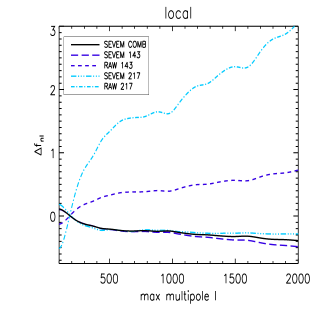
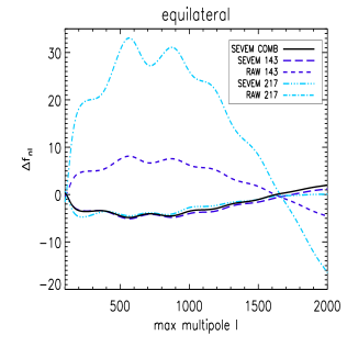
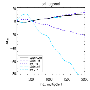
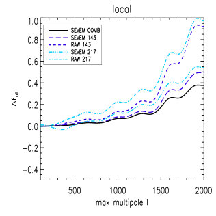
Figure 4: The bias ΔfnlΔsubscript𝑓nl\Delta f_{\rm nl} produced by the CIB-lensing bispectrum as a function of maxsubscriptmax\ell_{\rm max} for Planck cosmological frequencies (143 and 217 GHz). Solid lines correspond to the cleaned combined maps. Dash lines correspond to the raw map at 143 GHz and long dash lines correspond to the cleaned map at 143 GHz. Dash-and-dot lines correspond to the raw map at 217 GHz and dash-and-3-dots lines correspond to the cleaned map at 217 GHz. From left to right, we plot results for the local, equilateral and orthogonal fnlsubscript𝑓nlf_{\rm nl~{}}shapes.

3.2 Bispectrum

We derive the CIB–lensing, CMB and point sources bispectra for the three considered types of maps.

  • (i) Planck raw maps per frequency

    b123(𝙲𝙸𝙱𝙻𝚎𝚗𝚜,ν)=1(1+1)2(2+1)+3(3+1)2C3(𝙲𝙸𝙱𝙻𝚎𝚗𝚜,ν)C~1(𝙲𝙼𝙱)b1(ν)b2(ν)b3(ν)+(5perm),subscriptsuperscript𝑏𝙲𝙸𝙱𝙻𝚎𝚗𝚜𝜈subscript1subscript2subscript3subscript1subscript11subscript2subscript21subscript3subscript312subscriptsuperscript𝐶𝙲𝙸𝙱𝙻𝚎𝚗𝚜𝜈subscript3subscriptsuperscript~𝐶𝙲𝙼𝙱subscript1subscriptsuperscript𝑏𝜈subscript1superscriptsubscript𝑏subscript2𝜈superscriptsubscript𝑏subscript3𝜈5𝑝𝑒𝑟𝑚b^{({\mathtt{CIB-Lens}},\nu)}_{\ell_{1}\ell_{2}\ell_{3}}=\frac{\ell_{1}(\ell_{1}+1)-\ell_{2}(\ell_{2}+1)+\ell_{3}(\ell_{3}+1)}{2}C^{({\mathtt{CIB-Lens}},\nu)}_{\ell_{3}}\tilde{C}^{({\mathtt{CMB}})}_{\ell_{1}}b^{(\nu)}_{\ell_{1}}b_{\ell_{2}}^{(\nu)}b_{\ell_{3}}^{(\nu)}+(5~{}perm), (24)
    b123(𝙲𝙼𝙱,ν)=b1(ν)b2(ν)b3(ν)b123(𝙲𝙼𝙱),b123(ps,ν)=b1(ν)b2(ν)b3(ν)b(ps,ν).formulae-sequencesubscriptsuperscript𝑏𝙲𝙼𝙱𝜈subscript1subscript2subscript3superscriptsubscript𝑏subscript1𝜈superscriptsubscript𝑏subscript2𝜈superscriptsubscript𝑏subscript3𝜈subscriptsuperscript𝑏𝙲𝙼𝙱subscript1subscript2subscript3subscriptsuperscript𝑏ps𝜈subscript1subscript2subscript3superscriptsubscript𝑏subscript1𝜈superscriptsubscript𝑏subscript2𝜈superscriptsubscript𝑏subscript3𝜈superscript𝑏ps𝜈b^{({\mathtt{CMB}},\nu)}_{\ell_{1}\ell_{2}\ell_{3}}=b_{\ell_{1}}^{(\nu)}b_{\ell_{2}}^{(\nu)}b_{\ell_{3}}^{(\nu)}b^{({\mathtt{CMB}})}_{\ell_{1}\ell_{2}\ell_{3}},~{}~{}~{}~{}~{}b^{({{\rm ps}},\nu)}_{\ell_{1}\ell_{2}\ell_{3}}=b_{\ell_{1}}^{(\nu)}b_{\ell_{2}}^{(\nu)}b_{\ell_{3}}^{(\nu)}b^{({{\rm ps}},\nu)}. (25)
  • (ii) Planck cleaned maps per frequency

    b123(𝙲𝙸𝙱𝙻𝚎𝚗𝚜,𝚌𝚕𝚎𝚊𝚗,ν)=ijk=19fνi(ν)fνj(ν)fνk(ν)b1(νi)b2(νj)b3(νk)b123(𝙲𝙸𝙱𝙻𝚎𝚗𝚜,νiνjνk),subscriptsuperscript𝑏𝙲𝙸𝙱𝙻𝚎𝚗𝚜𝚌𝚕𝚎𝚊𝚗𝜈subscript1subscript2subscript3superscriptsubscript𝑖𝑗𝑘19subscriptsuperscript𝑓𝜈subscript𝜈𝑖subscriptsuperscript𝑓𝜈subscript𝜈𝑗subscriptsuperscript𝑓𝜈subscript𝜈𝑘subscriptsuperscript𝑏subscript𝜈𝑖subscript1superscriptsubscript𝑏subscript2subscript𝜈𝑗superscriptsubscript𝑏subscript3subscript𝜈𝑘subscriptsuperscript𝑏𝙲𝙸𝙱𝙻𝚎𝚗𝚜subscript𝜈𝑖subscript𝜈𝑗subscript𝜈𝑘subscript1subscript2subscript3b^{({\mathtt{CIB-Lens}},{\mathtt{clean}},\nu)}_{\ell_{1}\ell_{2}\ell_{3}}=\sum_{ijk=1}^{9}f^{(\nu)}_{\nu_{i}}f^{(\nu)}_{\nu_{j}}f^{(\nu)}_{\nu_{k}}b^{(\nu_{i})}_{\ell_{1}}b_{\ell_{2}}^{(\nu_{j})}b_{\ell_{3}}^{(\nu_{k})}b^{({\mathtt{CIB-Lens}},\nu_{i}\nu_{j}\nu_{k})}_{\ell_{1}\ell_{2}\ell_{3}}, (26)
    b123(𝙲𝙼𝙱,𝚌𝚕𝚎𝚊𝚗,ν)=ijk=19fνi(ν)fνj(ν)fνk(ν)b1(νi)b2(νj)b3(νk)b123(𝙲𝙼𝙱),b123(ps,𝚌𝚕𝚎𝚊𝚗,ν)=ijk=19fνi(ν)fνj(ν)fνk(ν)b1(νi)b2(νj)b3(νk)b(ps,νi,νj,νk).formulae-sequencesubscriptsuperscript𝑏𝙲𝙼𝙱𝚌𝚕𝚎𝚊𝚗𝜈subscript1subscript2subscript3superscriptsubscript𝑖𝑗𝑘19subscriptsuperscript𝑓𝜈subscript𝜈𝑖subscriptsuperscript𝑓𝜈subscript𝜈𝑗subscriptsuperscript𝑓𝜈subscript𝜈𝑘superscriptsubscript𝑏subscript1subscript𝜈𝑖superscriptsubscript𝑏subscript2subscript𝜈𝑗superscriptsubscript𝑏subscript3subscript𝜈𝑘subscriptsuperscript𝑏𝙲𝙼𝙱subscript1subscript2subscript3subscriptsuperscript𝑏ps𝚌𝚕𝚎𝚊𝚗𝜈subscript1subscript2subscript3superscriptsubscript𝑖𝑗𝑘19subscriptsuperscript𝑓𝜈subscript𝜈𝑖subscriptsuperscript𝑓𝜈subscript𝜈𝑗subscriptsuperscript𝑓𝜈subscript𝜈𝑘superscriptsubscript𝑏subscript1subscript𝜈𝑖superscriptsubscript𝑏subscript2subscript𝜈𝑗superscriptsubscript𝑏subscript3subscript𝜈𝑘superscript𝑏pssubscript𝜈𝑖subscript𝜈𝑗subscript𝜈𝑘b^{({\mathtt{CMB}},{\mathtt{clean}},\nu)}_{\ell_{1}\ell_{2}\ell_{3}}=\sum_{ijk=1}^{9}f^{(\nu)}_{\nu_{i}}f^{(\nu)}_{\nu_{j}}f^{(\nu)}_{\nu_{k}}b_{\ell_{1}}^{(\nu_{i})}b_{\ell_{2}}^{(\nu_{j})}b_{\ell_{3}}^{(\nu_{k})}b^{({\mathtt{CMB}})}_{\ell_{1}\ell_{2}\ell_{3}},~{}~{}~{}~{}~{}b^{({{\rm ps}},{\mathtt{clean}},\nu)}_{\ell_{1}\ell_{2}\ell_{3}}=\sum_{ijk=1}^{9}f^{(\nu)}_{\nu_{i}}f^{(\nu)}_{\nu_{j}}f^{(\nu)}_{\nu_{k}}b_{\ell_{1}}^{(\nu_{i})}b_{\ell_{2}}^{(\nu_{j})}b_{\ell_{3}}^{(\nu_{k})}b^{({{\rm ps}},\nu_{i},\nu_{j},\nu_{k})}. (27)
  • (iii) Planck combined cleaned maps

    b123(𝙲𝙸𝙱𝙻𝚎𝚗𝚜,𝚌𝚘𝚖𝚋)=ijk=19g1(νi)g2(νj)g3(νk)b1(νi)b2(νj)b3(νk)b123(𝙲𝙸𝙱𝙻𝚎𝚗𝚜,νiνjνk),subscriptsuperscript𝑏𝙲𝙸𝙱𝙻𝚎𝚗𝚜𝚌𝚘𝚖𝚋subscript1subscript2subscript3superscriptsubscript𝑖𝑗𝑘19subscriptsuperscript𝑔subscript𝜈𝑖subscript1subscriptsuperscript𝑔subscript𝜈𝑗subscript2subscriptsuperscript𝑔subscript𝜈𝑘subscript3subscriptsuperscript𝑏subscript𝜈𝑖subscript1superscriptsubscript𝑏subscript2subscript𝜈𝑗superscriptsubscript𝑏subscript3subscript𝜈𝑘subscriptsuperscript𝑏𝙲𝙸𝙱𝙻𝚎𝚗𝚜subscript𝜈𝑖subscript𝜈𝑗subscript𝜈𝑘subscript1subscript2subscript3b^{({\mathtt{CIB-Lens}},{\mathtt{comb}})}_{\ell_{1}\ell_{2}\ell_{3}}=\sum_{ijk=1}^{9}g^{(\nu_{i})}_{\ell_{1}}g^{(\nu_{j})}_{\ell_{2}}g^{(\nu_{k})}_{\ell_{3}}b^{(\nu_{i})}_{\ell_{1}}b_{\ell_{2}}^{(\nu_{j})}b_{\ell_{3}}^{(\nu_{k})}b^{({\mathtt{CIB-Lens}},\nu_{i}\nu_{j}\nu_{k})}_{\ell_{1}\ell_{2}\ell_{3}}, (28)
    b123(𝙲𝙼𝙱,𝚌𝚘𝚖𝚋)=ijk=19g1(νi)g2(νj)g3(νk)b1(νi)b2(νj)b3(νk)b123(𝙲𝙼𝙱),b123(ps,𝚌𝚘𝚖𝚋)=ijk=19g1(νi)g2(νj)g3(νk)b1(νi)b2(νj)b3(νk)b(ps,νi,νj,νk).formulae-sequencesubscriptsuperscript𝑏𝙲𝙼𝙱𝚌𝚘𝚖𝚋subscript1subscript2subscript3superscriptsubscript𝑖𝑗𝑘19subscriptsuperscript𝑔subscript𝜈𝑖subscript1subscriptsuperscript𝑔subscript𝜈𝑗subscript2subscriptsuperscript𝑔subscript𝜈𝑘subscript3superscriptsubscript𝑏subscript1subscript𝜈𝑖superscriptsubscript𝑏subscript2subscript𝜈𝑗superscriptsubscript𝑏subscript3subscript𝜈𝑘subscriptsuperscript𝑏𝙲𝙼𝙱subscript1subscript2subscript3subscriptsuperscript𝑏ps𝚌𝚘𝚖𝚋subscript1subscript2subscript3superscriptsubscript𝑖𝑗𝑘19subscriptsuperscript𝑔subscript𝜈𝑖subscript1subscriptsuperscript𝑔subscript𝜈𝑗subscript2subscriptsuperscript𝑔subscript𝜈𝑘subscript3superscriptsubscript𝑏subscript1subscript𝜈𝑖superscriptsubscript𝑏subscript2subscript𝜈𝑗superscriptsubscript𝑏subscript3subscript𝜈𝑘superscript𝑏pssubscript𝜈𝑖subscript𝜈𝑗subscript𝜈𝑘b^{({\mathtt{CMB}},{\mathtt{comb}})}_{\ell_{1}\ell_{2}\ell_{3}}=\sum_{ijk=1}^{9}g^{(\nu_{i})}_{\ell_{1}}g^{(\nu_{j})}_{\ell_{2}}g^{(\nu_{k})}_{\ell_{3}}b_{\ell_{1}}^{(\nu_{i})}b_{\ell_{2}}^{(\nu_{j})}b_{\ell_{3}}^{(\nu_{k})}b^{({\mathtt{CMB}})}_{\ell_{1}\ell_{2}\ell_{3}},~{}~{}~{}~{}~{}b^{({{\rm ps}},{\mathtt{comb}})}_{\ell_{1}\ell_{2}\ell_{3}}=\sum_{ijk=1}^{9}g^{(\nu_{i})}_{\ell_{1}}g^{(\nu_{j})}_{\ell_{2}}g^{(\nu_{k})}_{\ell_{3}}b_{\ell_{1}}^{(\nu_{i})}b_{\ell_{2}}^{(\nu_{j})}b_{\ell_{3}}^{(\nu_{k})}b^{({{\rm ps}},\nu_{i},\nu_{j},\nu_{k})}. (29)

b123(𝙲𝙼𝙱)subscriptsuperscript𝑏𝙲𝙼𝙱subscript1subscript2subscript3b^{({\mathtt{CMB}})}_{\ell_{1}\ell_{2}\ell_{3}} is the primordial bispectrum (see e.g. Curto et al., 2013, for the equations for the local, equilateral and orthogonal shapes). The term b123(𝙲𝙸𝙱𝙻𝚎𝚗𝚜,νiνjνk)subscriptsuperscript𝑏𝙲𝙸𝙱𝙻𝚎𝚗𝚜subscript𝜈𝑖subscript𝜈𝑗subscript𝜈𝑘subscript1subscript2subscript3b^{({\mathtt{CIB-Lens}},\nu_{i}\nu_{j}\nu_{k})}_{\ell_{1}\ell_{2}\ell_{3}} can be straightforwardly computed as a generalisation of the CIB-lensing bispectrum in Eq. (16) for three different frequencies

b123(𝙲𝙸𝙱𝙻𝚎𝚗𝚜,νiνjνk)1(1+1)2(2+1)+3(3+1)2C3(𝙲𝙸𝙱𝙻𝚎𝚗𝚜,νk)C~1(𝙲𝙼𝙱)+1(1+1)3(3+1)+2(2+1)2C2(𝙲𝙸𝙱𝙻𝚎𝚗𝚜,νj)C~1(𝙲𝙼𝙱)subscriptsuperscript𝑏𝙲𝙸𝙱𝙻𝚎𝚗𝚜subscript𝜈𝑖subscript𝜈𝑗subscript𝜈𝑘subscript1subscript2subscript3subscript1subscript11subscript2subscript21subscript3subscript312subscriptsuperscript𝐶𝙲𝙸𝙱𝙻𝚎𝚗𝚜subscript𝜈𝑘subscript3subscriptsuperscript~𝐶𝙲𝙼𝙱subscript1subscript1subscript11subscript3subscript31subscript2subscript212subscriptsuperscript𝐶𝙲𝙸𝙱𝙻𝚎𝚗𝚜subscript𝜈𝑗subscript2subscriptsuperscript~𝐶𝙲𝙼𝙱subscript1\displaystyle b^{({\mathtt{CIB-Lens}},\nu_{i}\nu_{j}\nu_{k})}_{\ell_{1}\ell_{2}\ell_{3}}\equiv\frac{\ell_{1}(\ell_{1}+1)-\ell_{2}(\ell_{2}+1)+\ell_{3}(\ell_{3}+1)}{2}C^{({\mathtt{CIB-Lens}},\nu_{k})}_{\ell_{3}}\tilde{C}^{({\mathtt{CMB}})}_{\ell_{1}}+\frac{\ell_{1}(\ell_{1}+1)-\ell_{3}(\ell_{3}+1)+\ell_{2}(\ell_{2}+1)}{2}C^{({\mathtt{CIB-Lens}},\nu_{j})}_{\ell_{2}}\tilde{C}^{({\mathtt{CMB}})}_{\ell_{1}}
+2(2+1)1(1+1)+3(3+1)2C3(𝙲𝙸𝙱𝙻𝚎𝚗𝚜,νk)C~2(𝙲𝙼𝙱)+3(3+1)1(1+1)+2(2+1)2C2(𝙲𝙸𝙱𝙻𝚎𝚗𝚜,νj)C~3(𝙲𝙼𝙱)subscript2subscript21subscript1subscript11subscript3subscript312subscriptsuperscript𝐶𝙲𝙸𝙱𝙻𝚎𝚗𝚜subscript𝜈𝑘subscript3subscriptsuperscript~𝐶𝙲𝙼𝙱subscript2subscript3subscript31subscript1subscript11subscript2subscript212subscriptsuperscript𝐶𝙲𝙸𝙱𝙻𝚎𝚗𝚜subscript𝜈𝑗subscript2subscriptsuperscript~𝐶𝙲𝙼𝙱subscript3\displaystyle+\frac{\ell_{2}(\ell_{2}+1)-\ell_{1}(\ell_{1}+1)+\ell_{3}(\ell_{3}+1)}{2}C^{({\mathtt{CIB-Lens}},\nu_{k})}_{\ell_{3}}\tilde{C}^{({\mathtt{CMB}})}_{\ell_{2}}+\frac{\ell_{3}(\ell_{3}+1)-\ell_{1}(\ell_{1}+1)+\ell_{2}(\ell_{2}+1)}{2}C^{({\mathtt{CIB-Lens}},\nu_{j})}_{\ell_{2}}\tilde{C}^{({\mathtt{CMB}})}_{\ell_{3}}
+2(2+1)3(3+1)+1(1+1)2C1(𝙲𝙸𝙱𝙻𝚎𝚗𝚜,νi)C~2(𝙲𝙼𝙱)+3(3+1)2(2+1)+1(1+1)2C1(𝙲𝙸𝙱𝙻𝚎𝚗𝚜,νi)C~3(𝙲𝙼𝙱).subscript2subscript21subscript3subscript31subscript1subscript112subscriptsuperscript𝐶𝙲𝙸𝙱𝙻𝚎𝚗𝚜subscript𝜈𝑖subscript1subscriptsuperscript~𝐶𝙲𝙼𝙱subscript2subscript3subscript31subscript2subscript21subscript1subscript112subscriptsuperscript𝐶𝙲𝙸𝙱𝙻𝚎𝚗𝚜subscript𝜈𝑖subscript1subscriptsuperscript~𝐶𝙲𝙼𝙱subscript3\displaystyle+\frac{\ell_{2}(\ell_{2}+1)-\ell_{3}(\ell_{3}+1)+\ell_{1}(\ell_{1}+1)}{2}C^{({\mathtt{CIB-Lens}},\nu_{i})}_{\ell_{1}}\tilde{C}^{({\mathtt{CMB}})}_{\ell_{2}}+\frac{\ell_{3}(\ell_{3}+1)-\ell_{2}(\ell_{2}+1)+\ell_{1}(\ell_{1}+1)}{2}C^{({\mathtt{CIB-Lens}},\nu_{i})}_{\ell_{1}}\tilde{C}^{({\mathtt{CMB}})}_{\ell_{3}}. (30)

Finally, the total point sources bispectrum b123(ps,νi,νj,νk)subscriptsuperscript𝑏pssubscript𝜈𝑖subscript𝜈𝑗subscript𝜈𝑘subscript1subscript2subscript3b^{({{\rm ps}},\nu_{i},\nu_{j},\nu_{k})}_{\ell_{1}\ell_{2}\ell_{3}} is computed from the standard prescription in terms of radio and CIB shot noise bispectra (see Appendix C for details on how we estimate shot noise bispectra of point sources when multiple frequencies are considered)

b123(ps,νi,νj,νk)=bsn(𝚁𝚊𝚍𝚒𝚘,νi,νj,νk)+bsn(𝙲𝙸𝙱,νi,νj,νk)C1(𝙲𝙸𝙱,νi)C2(𝙲𝙸𝙱,νj)C3(𝙲𝙸𝙱,νk)Csn(𝙲𝙸𝙱,νi)Csn(𝙲𝙸𝙱,νj)Csn(𝙲𝙸𝙱,νk).subscriptsuperscript𝑏pssubscript𝜈𝑖subscript𝜈𝑗subscript𝜈𝑘subscript1subscript2subscript3subscriptsuperscript𝑏𝚁𝚊𝚍𝚒𝚘subscript𝜈𝑖subscript𝜈𝑗subscript𝜈𝑘snsubscriptsuperscript𝑏𝙲𝙸𝙱subscript𝜈𝑖subscript𝜈𝑗subscript𝜈𝑘snsubscriptsuperscript𝐶𝙲𝙸𝙱subscript𝜈𝑖subscript1subscriptsuperscript𝐶𝙲𝙸𝙱subscript𝜈𝑗subscript2subscriptsuperscript𝐶𝙲𝙸𝙱subscript𝜈𝑘subscript3subscriptsuperscript𝐶𝙲𝙸𝙱subscript𝜈𝑖snsubscriptsuperscript𝐶𝙲𝙸𝙱subscript𝜈𝑗snsubscriptsuperscript𝐶𝙲𝙸𝙱subscript𝜈𝑘sn\displaystyle b^{({{\rm ps}},\nu_{i},\nu_{j},\nu_{k})}_{\ell_{1}\ell_{2}\ell_{3}}=b^{({\mathtt{Radio}},\nu_{i},\nu_{j},\nu_{k})}_{{\rm sn}}+b^{({\mathtt{CIB}},\nu_{i},\nu_{j},\nu_{k})}_{{\rm sn}}\sqrt{\frac{C^{({\mathtt{CIB}},\nu_{i})}_{\ell_{1}}C^{({\mathtt{CIB}},\nu_{j})}_{\ell_{2}}C^{({\mathtt{CIB}},\nu_{k})}_{\ell_{3}}}{C^{({\mathtt{CIB}},\nu_{i})}_{{\rm sn}}C^{({\mathtt{CIB}},\nu_{j})}_{{\rm sn}}C^{({\mathtt{CIB}},\nu_{k})}_{{\rm sn}}}}. (31)

Considering weak levels of non-Gaussianity, the bias induced in the primordial non-Gaussianity fnlsubscript𝑓nlf_{\rm nl~{}}due to a given target bispectrum B123(𝚝𝚊𝚛𝚐)subscriptsuperscript𝐵𝚝𝚊𝚛𝚐subscript1subscript2subscript3B^{({\mathtt{targ}})}_{\ell_{1}\ell_{2}\ell_{3}} is given by (see e.g. Lewis et al., 2011; Lacasa et al., 2012):

Δfnl=σ2(fnl)×123maxb123(𝚝𝚊𝚛𝚐)b123(𝚙𝚛𝚒𝚖)σ2(b123(𝚘𝚋𝚜)),Δsubscript𝑓nlsuperscript𝜎2subscript𝑓nlsuperscriptsubscriptsubscript1subscript2subscript3subscriptmaxsubscriptsuperscript𝑏𝚝𝚊𝚛𝚐subscript1subscript2subscript3subscriptsuperscript𝑏𝚙𝚛𝚒𝚖subscript1subscript2subscript3superscript𝜎2subscriptsuperscript𝑏𝚘𝚋𝚜subscript1subscript2subscript3\Delta f_{\rm nl}=\sigma^{2}\big{(}f_{\rm nl}\big{)}\times\sum_{\ell_{1}\leq\ell_{2}\leq\ell_{3}}^{\ell_{\rm max}}\frac{b^{({\mathtt{targ}})}_{\ell_{1}\ell_{2}\ell_{3}}b^{({\mathtt{prim}})}_{\ell_{1}\ell_{2}\ell_{3}}}{\sigma^{2}\big{(}b^{({\mathtt{obs}})}_{\ell_{1}\ell_{2}\ell_{3}}\big{)}}, (32)

where σ2(b123(𝚘𝚋𝚜))superscript𝜎2subscriptsuperscript𝑏𝚘𝚋𝚜subscript1subscript2subscript3\sigma^{2}\big{(}b^{({\mathtt{obs}})}_{\ell_{1}\ell_{2}\ell_{3}}\big{)} is the variance of the total observed bispectrum (Komatsu & Spergel, 2001)

σ2(b123(𝚘𝚋𝚜))superscript𝜎2subscriptsuperscript𝑏𝚘𝚋𝚜subscript1subscript2subscript3\displaystyle\sigma^{2}\big{(}b^{({\mathtt{obs}})}_{\ell_{1}\ell_{2}\ell_{3}}\big{)} b123(𝚘𝚋𝚜)b123(𝚘𝚋𝚜)b123(𝚘𝚋𝚜)b123(𝚘𝚋𝚜)1I1232Δ123C1C2C3,absentdelimited-⟨⟩subscriptsuperscript𝑏𝚘𝚋𝚜subscript1subscript2subscript3subscriptsuperscript𝑏𝚘𝚋𝚜subscript1subscript2subscript3delimited-⟨⟩subscriptsuperscript𝑏𝚘𝚋𝚜subscript1subscript2subscript3delimited-⟨⟩subscriptsuperscript𝑏𝚘𝚋𝚜subscript1subscript2subscript3similar-to-or-equals1superscriptsubscript𝐼subscript1subscript2subscript32subscriptΔsubscript1subscript2subscript3subscript𝐶subscript1subscript𝐶subscript2subscript𝐶subscript3\displaystyle\equiv\langle b^{({\mathtt{obs}})}_{\ell_{1}\ell_{2}\ell_{3}}b^{({\mathtt{obs}})}_{\ell_{1}\ell_{2}\ell_{3}}\rangle-\langle b^{({\mathtt{obs}})}_{\ell_{1}\ell_{2}\ell_{3}}\rangle\langle b^{({\mathtt{obs}})}_{\ell_{1}\ell_{2}\ell_{3}}\rangle\simeq\frac{1}{I_{\ell_{1}\ell_{2}\ell_{3}}^{2}}\Delta_{\ell_{1}\ell_{2}\ell_{3}}C_{\ell_{1}}C_{\ell_{2}}C_{\ell_{3}}, (33)
Δ123=1+2δ12δ23+δ12+δ23+δ13,subscriptΔsubscript1subscript2subscript312subscript𝛿subscript1subscript2subscript𝛿subscript2subscript3subscript𝛿subscript1subscript2subscript𝛿subscript2subscript3subscript𝛿subscript1subscript3\displaystyle\Delta_{\ell_{1}\ell_{2}\ell_{3}}=1+2\delta_{\ell_{1}\ell_{2}}\delta_{\ell_{2}\ell_{3}}+\delta_{\ell_{1}\ell_{2}}+\delta_{\ell_{2}\ell_{3}}+\delta_{\ell_{1}\ell_{3}}, (34)

Csubscript𝐶C_{\ell} is the total power spectrum of the map including CMB, CIB, radio sources and instrumental noise spectra and

I123(21+1)(22+1)(23+1)4π(123000).subscript𝐼subscript1subscript2subscript32subscript112subscript212subscript314𝜋subscript1subscript2subscript3000\displaystyle I_{\ell_{1}\ell_{2}\ell_{3}}\equiv\sqrt{\frac{\left(2\ell_{1}+1\right)\left(2\ell_{2}+1\right)\left(2\ell_{3}+1\right)}{4\pi}}\left(\begin{array}[]{ccc}\ell_{1}&\ell_{2}&\ell_{3}\\ 0&0&0\end{array}\right). (37)

Finally σ2(fnl)superscript𝜎2subscript𝑓nl\sigma^{2}\big{(}f_{\rm nl}\big{)} is the expected variance of the fnlsubscript𝑓nlf_{\rm nl~{}}parameter, given in terms of its Fisher matrix

σ2(fnl)=123max(b123(𝚙𝚛𝚒𝚖)I123)2σ2(b123(𝚘𝚋𝚜)).superscript𝜎2subscript𝑓nlsuperscriptsubscriptsubscript1subscript2subscript3subscriptmaxsuperscriptsubscriptsuperscript𝑏𝚙𝚛𝚒𝚖subscript1subscript2subscript3subscript𝐼subscript1subscript2subscript32superscript𝜎2subscriptsuperscript𝑏𝚘𝚋𝚜subscript1subscript2subscript3\sigma^{-2}\big{(}f_{\rm nl}\big{)}=\sum_{\ell_{1}\leq\ell_{2}\leq\ell_{3}}^{\ell_{\rm max}}\frac{\big{(}b^{({\mathtt{prim}})}_{\ell_{1}\ell_{2}\ell_{3}}I_{\ell_{1}\ell_{2}\ell_{3}}\big{)}^{2}}{\sigma^{2}\big{(}b^{({\mathtt{obs}})}_{\ell_{1}\ell_{2}\ell_{3}}\big{)}}. (38)

The values of σ2(fnl)superscript𝜎2subscript𝑓nl\sigma^{2}\big{(}f_{\rm nl}\big{)} for the different maps are given in Table 3. For the SEVEM combined map they agree well with the values published by Planck 2013 results XXIV (2014)666During the process of publication of this article the Planck Collaboration published new scientific results, in particular the first results on fnlsubscript𝑓𝑛𝑙f_{nl} with temperature and polarisation maps (Planck 2015 results XIX, 2015). No significant changes have been reported in the new Planck article regarding the results with temperature only.. Note that at 143 and 217 GHz, the component separation technique slightly increases the error on fnlsubscript𝑓nlf_{\rm nl}. This is due to the extra noise added by the template subtraction and it might be seen as the price to pay to have CMB cleaned maps.

3.3 fnlsubscript𝑓nlf_{\rm nl~{}}bias due to CIB–lensing and extragalactic sources bispectra

The bias ΔfnlΔsubscript𝑓nl\Delta f_{\rm nl} induced by the CIB-lensing correlation and unresolved extragalactic sources is estimated for the three types of maps previously described and for the local, equilateral and orthogonal fnlsubscript𝑓nlf_{\rm nl~{}}shapes in the frequency range between 100 and 353 GHz. Results are presented in Table 3 and Figure 4 for the CIB-lensing, and Table 4 and Figure 5 for the unresolved extragalactic sources.

For the frequency range considered here, the CIB-lensing bispectrum causes negligible bias in the primordial local and equilateral shapes with respect to the uncertainty on fnlsubscript𝑓nlf_{\rm nl} estimated by Eq. (38). The bias is also negligible for the orthogonal shape in the 100 and 143 GHz raw maps but reaches 2 and 3 σ𝜎\sigma detection levels for the 217 and 353 GHz raw maps respectively. The orthogonal bias is again negligible for the foreground-reduced maps at 143 and 217 GHz and the combined map (see Table 3 and Fig. 4). These results are explained as follows. Regarding the local shape, the CMB primordial signal peaks in squeezed configurations, such as (1,2,3)=(1000,1000,2)subscript1subscript2subscript3100010002(\ell_{1},\ell_{2},\ell_{3})=(1000,1000,2). However in this regime, the CIB-lensing bispectrum loses most of its amplitude (see top-left panel of Fig. 2). Regarding the equilateral shape, the CMB primordial signal is spread in configurations such that 1=2=3=subscript1subscript2subscript3\ell_{1}=\ell_{2}=\ell_{3}=\ell and becomes strongest at high resolution. The CIB-lensing bispectrum has some peaks in equilateral configurations (see bottom-left panel of Fig. 2) but they are located at low \ell and therefore they do not significantly couple with the CMB primordial equilateral signal. Finally regarding the orthogonal shape, the CMB primordial signal is peaked in configurations such as 2=3=21subscript2subscript32subscript1\ell_{2}=\ell_{3}=2\ell_{1} and 2=3=1subscript2subscript3subscript1\ell_{2}=\ell_{3}=\ell_{1} (Martínez-González & Planck Collaboration, 2012). They couple with the CIB-lensing signal producing an increasing bias for multipoles >500500\ell>500 (see Fig. 4). This explains the bias predicted for the raw channels at high frequency. The process of cleaning through the component separation subtracts part of the CIB signal and the bias for this shape is reduced in cleaned maps to about 30 per cent of the Planck uncertainty.

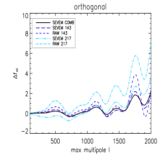
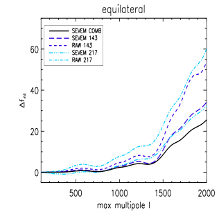
The unresolved extragalactic sources present levels of detection greater than 2σ2𝜎2\sigma at 353 GHz for the local, equilateral and orthogonal shapes due to the higher amplitude of IR sources at this frequency. There is a 2σ2𝜎2\sigma detection at 100 GHz for the equilateral shape which can be explained as a trace of the radio sources. The bias is again negligible for the foreground-reduced maps as the component separation technique is able to significantly reduce their contamination (see Table 4 and Fig. 5). These results are well in agreement with previous analyses from Lacasa et al. (2012) and Curto et al. (2013). These results are explained as follows. Regarding the local shape, the bispectrum of extragalactic sources does not have a significant signal in squeezed configurations at low frequencies (see top-left panel of Fig. 2) and therefore there we do not expected significant correlations with the CMB primordial local bispectrum. However the high frequency channels contain a significant contribution from IR sources in squeezed configurations that couple with the local CMB bispectrum. Regarding the equilateral shape, the extragalactic radio sources have significant signal in equilateral configurations (1=2=3subscript1subscript2subscript3\ell_{1}=\ell_{2}=\ell_{3}) at high multipoles (see bottom-left panel of Fig. 2) explaining the deviation seen in Table 4. The bispectrum of IR sources is dominant in equilateral configurations and at high multipoles explaining the large bias predicted at 353 GHz. Finally regarding the orthogonal shape, only the high frequency IR source bispectrum has a strong signal in configurations that couple with the CMB primordial orthogonal bispectrum, especially for high multipoles, explaining the large bias predicted at 353 GHz.
Refer to caption
Refer to caption
Refer to caption
Figure 5: The bias ΔfnlΔsubscript𝑓nl\Delta f_{\rm nl} produced by the point sources bispectrum as a function of maxsubscriptmax\ell_{\rm max} for Planck cosmological frequencies (143 and 217 GHz). Solid lines correspond to the cleaned combined maps. Dash lines correspond to the raw map at 143 GHz and long dash lines correspond to the cleaned map at 143 GHz. Dash-and-dot lines correspond to the raw map at 217 GHz and dash-and-3-dots lines correspond to the cleaned map at 217 GHz. From left to right, we plot results for the local, equilateral and orthogonal fnlsubscript𝑓nlf_{\rm nl~{}}shapes.
Table 4: Planck expected ΔfnlΔsubscript𝑓nl\Delta f_{\rm nl} bias due to unresolved point sources for the local, equilateral and orthogonal fnlsubscript𝑓nlf_{\rm nl~{}}shapes for max=subscriptmaxabsent\ell_{\rm max}=2000.
Frequency (GHz) 100 143 217 353 SEVEM 143 SEVEM 217 SEVEM combined
Local ΔfnlΔsubscript𝑓nl\Delta f_{\rm nl} 2.95 0.92 0.98 29.30 0.50 0.54 0.35
Local Δfnl/σ(fnl)Δsubscript𝑓nl𝜎subscript𝑓nl\Delta f_{\rm nl}/\sigma(f_{\rm nl}) 0.44 0.18 0.18 2.08 0.09 0.09 0.07
Equilateral ΔfnlΔsubscript𝑓nl\Delta f_{\rm nl} 160.07 54.20 60.32 1648.70 34.19 32.36 30.38
Equilateral Δfnl/σ(fnl)Δsubscript𝑓nl𝜎subscript𝑓nl\Delta f_{\rm nl}/\sigma(f_{\rm nl}) 2.10 0.79 0.85 12.25 0.48 0.45 0.45
Orthogonal ΔfnlΔsubscript𝑓nl\Delta f_{\rm nl} 10.53 2.45 7.00 553.01 1.87 3.56 2.94
Orthogonal Δfnl/σ(fnl)Δsubscript𝑓nl𝜎subscript𝑓nl\Delta f_{\rm nl}/\sigma(f_{\rm nl}) 0.27 0.07 0.20 7.24 0.05 0.10 0.09

4 Detectability of the CIB–Lensing bispectrum

In this section we develop statistical tools to detect the CIB–lensing bispectrum using an alternative approach to the widely known technique based on the cross-correlation of lensing potential reconstruction and temperature maps used for example in Planck 2013 results XVIII (2014) and Planck 2013 results XIX (2014). The cross-correlation approach followed in these publications used a lensing reconstruction based on quadratic combination of Planck CMB maps (Planck 2013 results XVII, 2014). The estimators that we propose in this article are directly defined in terms of cubic combinations of Planck maps where the CMB signal is dominant (100 to 217 GHz) and Planck maps where the CIB signal is dominant (217 to 857 GHz). Both approaches are linearly dependent and should result in similar levels of efficiency to detect the targeted CIB–lensing signal. The advantage of the new approach defined here is the application for the first time of a battery of well-known, efficient and optimal estimators widely used in the primordial bispectrum estimation to detect the CIB–lensing bispectrum. This approach has already been applied to the ISW–lensing estimation by Mangilli et al. (2013).

4.1 Single frequency bispectrum estimator

The optimal estimator for the amplitude of the CIB–lensing bispectrum, assuming small departures of non-Gaussianity, for the ideal, full–sky and isotropic instrumental noise is

A^(𝙲𝙸𝙱𝙻𝚎𝚗𝚜)=(F1)S^(𝙲𝙸𝙱𝙻𝚎𝚗𝚜)superscript^𝐴𝙲𝙸𝙱𝙻𝚎𝚗𝚜superscript𝐹1superscript^𝑆𝙲𝙸𝙱𝙻𝚎𝚗𝚜\hat{A}^{({\mathtt{CIB-Lens}})}=\big{(}F^{-1}\big{)}\hat{S}^{({\mathtt{CIB-Lens}})} (39)

where

S^(𝙲𝙸𝙱𝙻𝚎𝚗𝚜)=2123maxb123(𝚘𝚋𝚜)b123(𝙲𝙸𝙱𝙻𝚎𝚗𝚜)σ2(b123(𝚘𝚋𝚜)),superscript^𝑆𝙲𝙸𝙱𝙻𝚎𝚗𝚜superscriptsubscript2subscript1subscript2subscript3subscriptmaxsubscriptsuperscript𝑏𝚘𝚋𝚜subscript1subscript2subscript3subscriptsuperscript𝑏𝙲𝙸𝙱𝙻𝚎𝚗𝚜subscript1subscript2subscript3superscript𝜎2subscriptsuperscript𝑏𝚘𝚋𝚜subscript1subscript2subscript3\hat{S}^{({\mathtt{CIB-Lens}})}=\sum_{2\leq\ell_{1}\leq\ell_{2}\leq\ell_{3}}^{\ell_{\rm max}}\frac{b^{({\mathtt{obs}})}_{\ell_{1}\ell_{2}\ell_{3}}b^{({\mathtt{CIB-Lens}})}_{\ell_{1}\ell_{2}\ell_{3}}}{\sigma^{2}\big{(}b^{({\mathtt{obs}})}_{\ell_{1}\ell_{2}\ell_{3}}\big{)}}, (40)
F=2123maxb123(𝙲𝙸𝙱𝙻𝚎𝚗𝚜)b123(𝙲𝙸𝙱𝙻𝚎𝚗𝚜)σ2(b123(𝚘𝚋𝚜)),𝐹superscriptsubscript2subscript1subscript2subscript3subscriptmaxsubscriptsuperscript𝑏𝙲𝙸𝙱𝙻𝚎𝚗𝚜subscript1subscript2subscript3subscriptsuperscript𝑏𝙲𝙸𝙱𝙻𝚎𝚗𝚜subscript1subscript2subscript3superscript𝜎2subscriptsuperscript𝑏𝚘𝚋𝚜subscript1subscript2subscript3F=\sum_{2\leq\ell_{1}\leq\ell_{2}\leq\ell_{3}}^{\ell_{\rm max}}\frac{b^{({\mathtt{CIB-Lens}})}_{\ell_{1}\ell_{2}\ell_{3}}b^{({\mathtt{CIB-Lens}})}_{\ell_{1}\ell_{2}\ell_{3}}}{\sigma^{2}\big{(}b^{({\mathtt{obs}})}_{\ell_{1}\ell_{2}\ell_{3}}\big{)}}, (41)

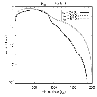
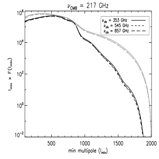
and the observed bispectrum b123(𝚘𝚋𝚜)subscriptsuperscript𝑏𝚘𝚋𝚜subscript1subscript2subscript3b^{({\mathtt{obs}})}_{\ell_{1}\ell_{2}\ell_{3}} is based on cubic combinations of Planck data in the amsubscript𝑎𝑚a_{\ell m} decomposition on the sphere. Another interesting quantity is the expected bispectrum signal-to-noise ratio as a function of the largest scale mode minsubscriptmin\ell_{\rm min} (Lewis et al., 2011):

Fmin=min123maxb123(𝙲𝙸𝙱𝙻𝚎𝚗𝚜)b123(𝙲𝙸𝙱𝙻𝚎𝚗𝚜)σ2(b123(𝚘𝚋𝚜)),subscript𝐹subscriptminsuperscriptsubscriptsubscriptminsubscript1subscript2subscript3subscriptmaxsubscriptsuperscript𝑏𝙲𝙸𝙱𝙻𝚎𝚗𝚜subscript1subscript2subscript3subscriptsuperscript𝑏𝙲𝙸𝙱𝙻𝚎𝚗𝚜subscript1subscript2subscript3superscript𝜎2subscriptsuperscript𝑏𝚘𝚋𝚜subscript1subscript2subscript3F_{\ell_{\rm min}}=\sum_{\ell_{\rm min}\leq\ell_{1}\leq\ell_{2}\leq\ell_{3}}^{\ell_{\rm max}}\frac{b^{({\mathtt{CIB-Lens}})}_{\ell_{1}\ell_{2}\ell_{3}}b^{({\mathtt{CIB-Lens}})}_{\ell_{1}\ell_{2}\ell_{3}}}{\sigma^{2}\big{(}b^{({\mathtt{obs}})}_{\ell_{1}\ell_{2}\ell_{3}}\big{)}}, (42)

This quantity helps to find the multipole configurations where the bispectrum signal peaks.

The signal-to-noise ratio of the CIB–lensing signal of this estimator F𝐹\sqrt{F} is summarised in Table 5 for the frequency range between 100 and 857 GHz and max=subscriptmaxabsent\ell_{\rm max}=2000 and different sky fractions available: 100% (full sky), 30.4%777This is the percentage of available sky used in the main results of Planck 2013 results XVIII (2014). and 10%. We compute this ratio considering the CIB–lensing signal alone (Eq. 41) and the joint Fisher matrix for the four non-primordial bispectra used in this article, i.e, CIB–lensing, ISW–lensing, CIB, and extragalactic point sources, by using the generalised Fisher matrix between the bispectra i𝑖i and j𝑗j:

Fij=2123maxb123(i)b123(j)σ2(b123(𝚘𝚋𝚜)).subscript𝐹𝑖𝑗superscriptsubscript2subscript1subscript2subscript3subscriptmaxsubscriptsuperscript𝑏𝑖subscript1subscript2subscript3subscriptsuperscript𝑏𝑗subscript1subscript2subscript3superscript𝜎2subscriptsuperscript𝑏𝚘𝚋𝚜subscript1subscript2subscript3F_{ij}=\sum_{2\leq\ell_{1}\leq\ell_{2}\leq\ell_{3}}^{\ell_{\rm max}}\frac{b^{(i)}_{\ell_{1}\ell_{2}\ell_{3}}b^{(j)}_{\ell_{1}\ell_{2}\ell_{3}}}{\sigma^{2}\big{(}b^{({\mathtt{obs}})}_{\ell_{1}\ell_{2}\ell_{3}}\big{)}}. (43)

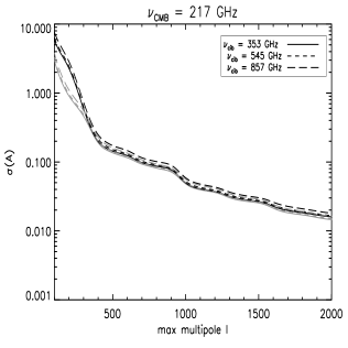
The first case is simply Findep=Fiisubscript𝐹𝑖𝑛𝑑𝑒𝑝subscript𝐹𝑖𝑖F_{indep}=F_{ii} whereas the second is Fjoint=1/(F1)iisubscript𝐹𝑗𝑜𝑖𝑛𝑡1subscriptsuperscript𝐹1𝑖𝑖F_{joint}=1/\left(F^{-1}\right)_{ii} with i𝑖i being the CIB–lensing case. The significance level for the detection of the CIB–lensing signal with this estimator increases from approx. 0.5σ𝜎\sigma at 100 GHz to 9.8σ𝜎\sigma at 353 GHz considering the full sky available. In a more realistic scenario with a 10% sky available for the CIB maps, the CIB–lensing signal would be detected with a maximum precision of 1σ𝜎\sigma at 353 GHz. At higher frequencies, the CIB spectrum dominates in the denominator in Eq. (41) leading to low significance levels of detection for the CIB–lensing bispectrum.

Table 5: Signal-to-noise ratio F𝐹\sqrt{F} of the amplitude of the CIB–lensing bispectrum for the Planck raw maps at frequencies between 100 and 857 GHz using ideal conditions (isotropic instrumental noise) from the Fisher matrix in Eq. (41) and several sky fractions available.
Frequency (GHz) 100 143 217 353 545 857
Findep1/2(fsky=1)superscriptsubscript𝐹𝑖𝑛𝑑𝑒𝑝12subscript𝑓𝑠𝑘𝑦1F_{indep}^{1/2}\left(f_{sky}=1\right) 0.55 1.80 7.57 10.19 0.25 0.00
Findep1/2(fsky=0.304)superscriptsubscript𝐹𝑖𝑛𝑑𝑒𝑝12subscript𝑓𝑠𝑘𝑦0.304F_{indep}^{1/2}\left(f_{sky}=0.304\right) 0.17 0.55 2.30 3.10 0.08 0.00
Findep1/2(fsky=0.100)superscriptsubscript𝐹𝑖𝑛𝑑𝑒𝑝12subscript𝑓𝑠𝑘𝑦0.100F_{indep}^{1/2}\left(f_{sky}=0.100\right) 0.06 0.18 0.76 1.02 0.03 0.00
Fjoint1/2(fsky=1)superscriptsubscript𝐹𝑗𝑜𝑖𝑛𝑡12subscript𝑓𝑠𝑘𝑦1F_{joint}^{1/2}\left(f_{sky}=1\right) 0.52 1.66 6.87 9.80 0.25 0.00
Fjoint1/2(fsky=0.304)superscriptsubscript𝐹𝑗𝑜𝑖𝑛𝑡12subscript𝑓𝑠𝑘𝑦0.304F_{joint}^{1/2}\left(f_{sky}=0.304\right) 0.16 0.51 2.09 2.98 0.07 0.00
Fjoint1/2(fsky=0.100)superscriptsubscript𝐹𝑗𝑜𝑖𝑛𝑡12subscript𝑓𝑠𝑘𝑦0.100F_{joint}^{1/2}\left(f_{sky}=0.100\right) 0.05 0.17 0.69 0.98 0.02 0.00

4.2 Asymmetric estimator for CMB–CIB correlated maps

At high Planck frequencies the CIB bispectrum could strongly limit our capability to detect the CIB–lensing signal, as well as the ISW–lensing contribution could be a relevant “noise” at 100–217 GHz. Therefore, a more feasible procedure to detect the CIB–lensing bispectrum signal should correlate CMB signal-dominated maps and CIB signal-dominated maps. We define an estimator for the CIB-lensing signal by considering the asymmetric configuration a~1m1(𝚛𝚊𝚠,ν𝙲𝙼𝙱)a~2m2(𝚛𝚊𝚠,ν𝙲𝙼𝙱)a3m3(𝚛𝚊𝚠,ν𝙲𝙸𝙱)subscriptsuperscript~𝑎𝚛𝚊𝚠subscript𝜈𝙲𝙼𝙱subscript1subscript𝑚1subscriptsuperscript~𝑎𝚛𝚊𝚠subscript𝜈𝙲𝙼𝙱subscript2subscript𝑚2subscriptsuperscript𝑎𝚛𝚊𝚠subscript𝜈𝙲𝙸𝙱subscript3subscript𝑚3\tilde{a}^{({\mathtt{raw}},\nu_{\mathtt{CMB}})}_{\ell_{1}m_{1}}\tilde{a}^{({\mathtt{raw}},\nu_{\mathtt{CMB}})}_{\ell_{2}m_{2}}a^{({\mathtt{raw}},\nu_{\mathtt{CIB}})}_{\ell_{3}m_{3}} where ν𝙲𝙼𝙱subscript𝜈𝙲𝙼𝙱\nu_{\mathtt{CMB}} and ν𝙲𝙸𝙱subscript𝜈𝙲𝙸𝙱\nu_{\mathtt{CIB}} are frequency channels where the CMB and CIB signal are significant respectively. We consider ν𝙲𝙼𝙱=subscript𝜈𝙲𝙼𝙱absent\nu_{\mathtt{CMB}}= 100, 143 and 217 GHz and ν𝙲𝙸𝙱=subscript𝜈𝙲𝙸𝙱absent\nu_{\mathtt{CIB}}= 217, 353, 545 and 857 GHz. The four non-primordial averaged bispectra considered in this paper, namely the radio, CIB, CIB-lensing and ISW-lensing bispectra, are written in this asymmetric configuration by:

b123(𝚁𝚊𝚍𝚒𝚘)=bsn(𝚁𝚊𝚍𝚒𝚘,ν𝙲𝙼𝙱,ν𝙲𝙼𝙱,ν𝙲𝙸𝙱)subscriptsuperscript𝑏𝚁𝚊𝚍𝚒𝚘subscript1subscript2subscript3subscriptsuperscript𝑏𝚁𝚊𝚍𝚒𝚘subscript𝜈𝙲𝙼𝙱subscript𝜈𝙲𝙼𝙱subscript𝜈𝙲𝙸𝙱snb^{({\mathtt{Radio}})}_{\ell_{1}\ell_{2}\ell_{3}}=b^{({\mathtt{Radio}},\nu_{\mathtt{CMB}},\nu_{\mathtt{CMB}},\nu_{\mathtt{CIB}})}_{{\rm sn}} (44)
b123(𝙲𝙸𝙱)=bsn(𝙲𝙸𝙱,ν𝙲𝙼𝙱,ν𝙲𝙼𝙱,ν𝙲𝙸𝙱)C1(𝙲𝙸𝙱,ν𝙲𝙼𝙱)C2(𝙲𝙸𝙱,ν𝙲𝙼𝙱)C3(𝙲𝙸𝙱,ν𝙲𝙸𝙱)Csn(𝙲𝙸𝙱,ν𝙲𝙼𝙱)Csn(𝙲𝙸𝙱,ν𝙲𝙼𝙱)Csn(𝙲𝙸𝙱,ν𝙲𝙸𝙱)subscriptsuperscript𝑏𝙲𝙸𝙱subscript1subscript2subscript3subscriptsuperscript𝑏𝙲𝙸𝙱subscript𝜈𝙲𝙼𝙱subscript𝜈𝙲𝙼𝙱subscript𝜈𝙲𝙸𝙱snsubscriptsuperscript𝐶𝙲𝙸𝙱subscript𝜈𝙲𝙼𝙱subscript1subscriptsuperscript𝐶𝙲𝙸𝙱subscript𝜈𝙲𝙼𝙱subscript2subscriptsuperscript𝐶𝙲𝙸𝙱subscript𝜈𝙲𝙸𝙱subscript3subscriptsuperscript𝐶𝙲𝙸𝙱subscript𝜈𝙲𝙼𝙱snsubscriptsuperscript𝐶𝙲𝙸𝙱subscript𝜈𝙲𝙼𝙱snsubscriptsuperscript𝐶𝙲𝙸𝙱subscript𝜈𝙲𝙸𝙱snb^{({\mathtt{CIB}})}_{\ell_{1}\ell_{2}\ell_{3}}=b^{({\mathtt{CIB}},\nu_{\mathtt{CMB}},\nu_{\mathtt{CMB}},\nu_{\mathtt{CIB}})}_{{\rm sn}}\sqrt{\frac{C^{({\mathtt{CIB}},\nu_{\mathtt{CMB}})}_{\ell_{1}}C^{({\mathtt{CIB}},\nu_{\mathtt{CMB}})}_{\ell_{2}}C^{({\mathtt{CIB}},\nu_{\mathtt{CIB}})}_{\ell_{3}}}{C^{({\mathtt{CIB}},\nu_{\mathtt{CMB}})}_{{\rm sn}}C^{({\mathtt{CIB}},\nu_{\mathtt{CMB}})}_{{\rm sn}}C^{({\mathtt{CIB}},\nu_{\mathtt{CIB}})}_{{\rm sn}}}} (45)
b123(𝙲𝙸𝙱𝙻𝚎𝚗𝚜)=subscriptsuperscript𝑏𝙲𝙸𝙱𝙻𝚎𝚗𝚜subscript1subscript2subscript3absent\displaystyle b^{({\mathtt{CIB-Lens}})}_{\ell_{1}\ell_{2}\ell_{3}}=
[1(1+1)2(2+1)+3(3+1)2C~1(𝙲𝙼𝙱)C3(𝙲𝙸𝙱𝙻𝚎𝚗𝚜,ν𝙲𝙸𝙱)+2(2+1)1(1+1)+3(3+1)2C~2(𝙲𝙼𝙱)C3(𝙲𝙸𝙱𝙻𝚎𝚗𝚜,ν𝙲𝙸𝙱)],delimited-[]subscript1subscript11subscript2subscript21subscript3subscript312subscriptsuperscript~𝐶𝙲𝙼𝙱subscript1subscriptsuperscript𝐶𝙲𝙸𝙱𝙻𝚎𝚗𝚜subscript𝜈𝙲𝙸𝙱subscript3subscript2subscript21subscript1subscript11subscript3subscript312subscriptsuperscript~𝐶𝙲𝙼𝙱subscript2subscriptsuperscript𝐶𝙲𝙸𝙱𝙻𝚎𝚗𝚜subscript𝜈𝙲𝙸𝙱subscript3\displaystyle\bigg{[}{\ell_{1}(\ell_{1}+1)-\ell_{2}(\ell_{2}+1)+\ell_{3}(\ell_{3}+1)\over 2}\,\tilde{C}^{({\mathtt{CMB}})}_{\ell_{1}}\,C^{({\mathtt{CIB-Lens}},\nu_{\mathtt{CIB}})}_{\ell_{3}}+{\ell_{2}(\ell_{2}+1)-\ell_{1}(\ell_{1}+1)+\ell_{3}(\ell_{3}+1)\over 2}\,\tilde{C}^{({\mathtt{CMB}})}_{\ell_{2}}\,C^{({\mathtt{CIB-Lens}},\nu_{\mathtt{CIB}})}_{\ell_{3}}\bigg{]}\,, (46)

and

b123(𝙸𝚂𝚆𝙻𝚎𝚗𝚜)=[1(1+1)2(2+1)+3(3+1)2C~1(𝙲𝙼𝙱)C3(𝙸𝚂𝚆𝙻𝚎𝚗𝚜)+(5perm)].subscriptsuperscript𝑏𝙸𝚂𝚆𝙻𝚎𝚗𝚜subscript1subscript2subscript3delimited-[]subscript1subscript11subscript2subscript21subscript3subscript312subscriptsuperscript~𝐶𝙲𝙼𝙱subscript1subscriptsuperscript𝐶𝙸𝚂𝚆𝙻𝚎𝚗𝚜subscript35𝑝𝑒𝑟𝑚\displaystyle b^{({\mathtt{ISW-Lens}})}_{\ell_{1}\ell_{2}\ell_{3}}=\bigg{[}{\ell_{1}(\ell_{1}+1)-\ell_{2}(\ell_{2}+1)+\ell_{3}(\ell_{3}+1)\over 2}\,\tilde{C}^{({\mathtt{CMB}})}_{\ell_{1}}\,C^{({\mathtt{ISW-Lens}})}_{\ell_{3}}+(5~{}perm)\bigg{]}. (47)

The covariance matrix is nearly diagonal and can be approximated by the following expression (see Appendix D) for the CMB x CMB x CIB configurations:

σ2(b123(𝚘𝚋𝚜))=1I1232C~1(𝙲𝙼𝙱)C~2(𝙲𝙼𝙱)C3(𝙲𝙸𝙱)(1+δ12).superscript𝜎2subscriptsuperscript𝑏𝚘𝚋𝚜subscript1subscript2subscript31superscriptsubscript𝐼subscript1subscript2subscript32subscriptsuperscript~𝐶𝙲𝙼𝙱subscript1subscriptsuperscript~𝐶𝙲𝙼𝙱subscript2subscriptsuperscript𝐶𝙲𝙸𝙱subscript31subscript𝛿subscript1subscript2\displaystyle\sigma^{2}\big{(}b^{({\mathtt{obs}})}_{\ell_{1}\ell_{2}\ell_{3}}\big{)}=\frac{1}{I_{\ell_{1}\ell_{2}\ell_{3}}^{2}}\tilde{C}^{({\mathtt{CMB}})}_{\ell_{1}}\tilde{C}^{({\mathtt{CMB}})}_{\ell_{2}}C^{({\mathtt{CIB}})}_{\ell_{3}}\left(1+\delta_{\ell_{1}\ell_{2}}\right). (48)

The CIB-lensing estimator for this configuration is now:

S^(𝙲𝙸𝙱𝙻𝚎𝚗𝚜)=212,3maxb123(𝚘𝚋𝚜)b123(𝙲𝙸𝙱𝙻𝚎𝚗𝚜)σ2(b123(𝚘𝚋𝚜)).superscript^𝑆𝙲𝙸𝙱𝙻𝚎𝚗𝚜superscriptsubscriptformulae-sequence2subscript1subscript2subscript3subscriptmaxsubscriptsuperscript𝑏𝚘𝚋𝚜subscript1subscript2subscript3subscriptsuperscript𝑏𝙲𝙸𝙱𝙻𝚎𝚗𝚜subscript1subscript2subscript3superscript𝜎2subscriptsuperscript𝑏𝚘𝚋𝚜subscript1subscript2subscript3\hat{S}^{({\mathtt{CIB-Lens}})}=\sum_{2\leq\ell_{1}\leq\ell_{2},\ell_{3}}^{\ell_{\rm max}}\frac{b^{({\mathtt{obs}})}_{\ell_{1}\ell_{2}\ell_{3}}b^{({\mathtt{CIB-Lens}})}_{\ell_{1}\ell_{2}\ell_{3}}}{\sigma^{2}\big{(}b^{({\mathtt{obs}})}_{\ell_{1}\ell_{2}\ell_{3}}\big{)}}. (49)

The estimator is different with respect to the single map estimators since it admits more configurations because we just have symmetry under permutations of 1subscript1\ell_{1} and 2subscript2\ell_{2} whereas 3subscript3\ell_{3} is free. The Fisher matrix for the four bispectra considered in this work is defined as (Komatsu & Spergel, 2001):

Fij=212,3maxb123(i)b123(j)σ2(b123(𝚘𝚋𝚜))subscript𝐹𝑖𝑗superscriptsubscriptformulae-sequence2subscript1subscript2subscript3subscriptmaxsubscriptsuperscript𝑏𝑖subscript1subscript2subscript3subscriptsuperscript𝑏𝑗subscript1subscript2subscript3superscript𝜎2subscriptsuperscript𝑏𝚘𝚋𝚜subscript1subscript2subscript3F_{ij}=\sum_{2\leq\ell_{1}\leq\ell_{2},\ell_{3}}^{\ell_{\rm max}}\frac{b^{(i)}_{\ell_{1}\ell_{2}\ell_{3}}b^{(j)}_{\ell_{1}\ell_{2}\ell_{3}}}{\sigma^{2}\big{(}b^{({\mathtt{obs}})}_{\ell_{1}\ell_{2}\ell_{3}}\big{)}} (50)

where the indices i𝑖i and j𝑗j cover the following bispectra: (1) radio, (2) CIB, (3) CIB-lensing and (4) ISW-lensing. We also define the Fisher matrix in terms of the minimum multipole minsubscriptmin\ell_{\rm min}:

(Fij)min=min12,3maxb123(i)b123(j)σ2(b123(𝚘𝚋𝚜)).subscriptsubscript𝐹𝑖𝑗subscriptminsuperscriptsubscriptformulae-sequencesubscriptminsubscript1subscript2subscript3subscriptmaxsubscriptsuperscript𝑏𝑖subscript1subscript2subscript3subscriptsuperscript𝑏𝑗subscript1subscript2subscript3superscript𝜎2subscriptsuperscript𝑏𝚘𝚋𝚜subscript1subscript2subscript3\left(F_{ij}\right)_{\ell_{\rm min}}=\sum_{\ell_{\rm min}\leq\ell_{1}\leq\ell_{2},\ell_{3}}^{\ell_{\rm max}}\frac{b^{(i)}_{\ell_{1}\ell_{2}\ell_{3}}b^{(j)}_{\ell_{1}\ell_{2}\ell_{3}}}{\sigma^{2}\big{(}b^{({\mathtt{obs}})}_{\ell_{1}\ell_{2}\ell_{3}}\big{)}}\,. (51)

The Cramér-Rao inequality states that the inverse of the Fisher information matrix is a lower bound on the variance of any unbiased estimator in the best optimal conditions. Therefore the variance of the amplitude of each bispectra can be obtained by inverting the Fisher matrix

σjoint2(Ai)=(F1)ii.superscriptsubscript𝜎joint2subscript𝐴𝑖subscriptsuperscript𝐹1𝑖𝑖\sigma_{\rm joint}^{2}(A_{i})=\left(F^{-1}\right)_{ii}. (52)

This approach performs a joint analysis including the correlations among the four types of bispectra, in comparison to the independent constraint that would have a lower variance:

σindep2(Ai)=(Fii)1.superscriptsubscript𝜎indep2subscript𝐴𝑖superscriptsubscript𝐹𝑖𝑖1\sigma_{\rm indep}^{2}(A_{i})=\left(F_{ii}\right)^{-1}. (53)

The signal-to-noise ratio is given by:

Findep1/2(Ai)=Fii1/2Fjoint1/2(Ai)=1/(F1)ii.formulae-sequencesuperscriptsubscript𝐹indep12subscript𝐴𝑖subscriptsuperscript𝐹12𝑖𝑖superscriptsubscript𝐹joint12subscript𝐴𝑖1subscriptsuperscript𝐹1𝑖𝑖F_{\rm indep}^{1/2}(A_{i})=F^{1/2}_{ii}~{}~{}~{}~{}~{}~{}~{}~{}~{}~{}~{}~{}~{}~{}~{}~{}~{}~{}F_{\rm joint}^{1/2}(A_{i})=1/\sqrt{\left(F^{-1}\right)_{ii}}. (54)

The expected uncertainties for the CIB-lensing estimator, computed both using the independent and the joint approach, are plotted in Fig. 6 and is summarised in Table 6 for max=subscriptmaxabsent\ell_{\rm max}=2000. In an ideal scenario where the CMB and the CIB maps are completely separated in two full sky maps, we would have a detectability level of approximately 63σ63𝜎63\sigma in the best configurations given in Table 6 for max=subscriptmaxabsent\ell_{\rm max}=2000. However available CIB maps cover only about 10% of the sky (Planck 2013 results XXX, 2014) in the best case scenarios. For the incomplete sky case, the detectability level of the bispectrum is rescaled by the fraction of the available sky fskysubscript𝑓skyf_{{\rm{sky}}} such that σ(A)σ(A)/fsky𝜎𝐴𝜎𝐴subscript𝑓sky\sigma(A)\longrightarrow\sigma(A)/\sqrt{f_{{\rm{sky}}}}. As the CIB–lensing bispectrum is not squeezed (see Fig. 6), this case is not affected by the loss of low multipoles, which are unobservable for small sky fractions, so this approximation is safe up to the mentioned 10% of the sky. This would provide detectability levels between 12σ𝜎\sigma to 20σ𝜎\sigma respectively for a mask with 10% of the sky available using the joint estimator (see Table 6).
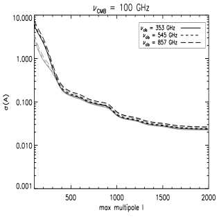
Refer to caption
Refer to caption
Refer to caption
Refer to caption
Refer to caption
Refer to caption
Figure 6: Top: the uncertainty for the CIB–lensing bispectrum amplitude σ(A)𝜎𝐴\sigma(A) as a function of maxsubscriptmax\ell_{\rm max} for cleaned CMB maps (at 100, 143 and 217 GHz) combined with CIB dominated maps at 353, 545 and 857 GHz using the independent estimates (grey lines) and using the joint estimates (black lines). Bottom: the Fischer matrix Fminsubscript𝐹subscriptminF_{\ell_{\rm min}} (multiplied by minsubscriptmin\ell_{\rm min}) as a function of minsubscriptmin\ell_{\rm min} for the same cases as above.
Table 6: The signal-to-noise ratio F𝐹\sqrt{F} of the amplitude of the CIB–lensing bispectrum for clean full–sky maps using the joint (Eq. 52) and independent (Eq. 54) Fisher matrices for the combinations the clean CMB at frequencies between 100 and 217 GHz and the clean CIB at frequencies between 353 and 857 GHz using 100%, (30.4%), [10%] of the sky..
Case Frequency ν𝙲𝙸𝙱subscript𝜈𝙲𝙸𝙱\nu_{{\mathtt{CIB}}} = 353 GHz ν𝙲𝙸𝙱subscript𝜈𝙲𝙸𝙱\nu_{{\mathtt{CIB}}} = 545 GHz ν𝙲𝙸𝙱subscript𝜈𝙲𝙸𝙱\nu_{{\mathtt{CIB}}} = 857 GHz
Joint ν𝙲𝙼𝙱subscript𝜈𝙲𝙼𝙱\nu_{{\mathtt{CMB}}} = 100 GHz 42.70 ( 23.54) [ 13.50] 41.03 ( 22.62) [ 12.98] 37.60 ( 20.73) [ 11.89]
Joint ν𝙲𝙼𝙱subscript𝜈𝙲𝙼𝙱\nu_{{\mathtt{CMB}}} = 143 GHz 62.66 ( 34.55) [ 19.82] 60.15 ( 33.17) [ 19.02] 55.40 ( 30.54) [ 17.52]
Joint ν𝙲𝙼𝙱subscript𝜈𝙲𝙼𝙱\nu_{{\mathtt{CMB}}} = 217 GHz 62.37 ( 34.39) [ 19.72] 59.90 ( 33.03) [ 18.94] 55.19 ( 30.43) [ 17.45]
Independent ν𝙲𝙼𝙱subscript𝜈𝙲𝙼𝙱\nu_{{\mathtt{CMB}}} = 100 GHz 44.65 ( 24.62) [ 14.12] 43.21 ( 23.83) [ 13.66] 39.71 ( 21.90) [ 12.56]
Independent ν𝙲𝙼𝙱subscript𝜈𝙲𝙼𝙱\nu_{{\mathtt{CMB}}} = 143 GHz 68.70 ( 37.88) [ 21.73] 66.61 ( 36.73) [ 21.06] 61.42 ( 33.86) [ 19.42]
Independent ν𝙲𝙼𝙱subscript𝜈𝙲𝙼𝙱\nu_{{\mathtt{CMB}}} = 217 GHz 68.51 ( 37.77) [ 21.66] 66.42 ( 36.62) [ 21.00] 61.26 ( 33.78) [ 19.37]

We have compared our results with the estimates of the CIB–lensing correlation published in Planck 2013 results XVIII (2014). The statistical estimator used in that work is based on a cross-correlation between the lensing potential in harmonic space, ϕmsubscriptitalic-ϕ𝑚\phi_{\ell m}, and a temperature map. The amplitude of the detection is obtained with the quadrature sum of the significance of the different multipole bins. This amplitude takes into account effects such as correlations among different bins but no systematic errors or point source corrections. The final estimates presented in that paper are computed using the lensing reconstruction at 143 GHz and the Planck HFI foreground reduced maps with a mask of 30.4% of available sky. The results obtained in this way and our predictions for the same configuration are given in Table 7. Planck 2013 results XVIII (2014) provides two types of detection significances: one that only includes the statistical errors only and another one that includes statistical and systematic errors. Compared to the first one – as we do not consider systematic errors here – the detection significance by Planck 2013 results XVIII (2014) and our model are nearly equivalent for the 353 to 857 GHz range. Note that the values measured by Planck 2013 results XVIII (2014) are quite sensitive to the systematic effects (see Table 7). We have additionally repeated our analysis without adding instrumental noise, i.e. for ideal conditions, and have found F=𝐹absent\sqrt{F}= 39, 38, 35 for the 353, 545 and 857 GHz bands. Both cases show a decreasing trend in the signal-to-noise level of the CIB-lensing correlation as we increase the frequency, due to the higher contamination of the CIB. We do not see a peak at 545 GHz, and we think that the peak observed in Planck 2013 results XVIII (2014) at 545 GHz might be explained by an unknown systematic artefact present in the data.

Table 7: Significance of the amplitude of the CIB–lensing correlation using the lensing reconstruction at 143 GHz and the Planck HFI foreground reduced maps with a mask of 30.4% of available sky. Top line: measurements by Planck 2013 results XVIII (2014). Bottom line: our predictions for an optimal bispectrum estimator for the same configuration.
Case ν𝙲𝙸𝙱subscript𝜈𝙲𝙸𝙱\nu_{{\mathtt{CIB}}} = 353 GHz ν𝙲𝙸𝙱subscript𝜈𝙲𝙸𝙱\nu_{{\mathtt{CIB}}} = 545 GHz ν𝙲𝙸𝙱subscript𝜈𝙲𝙸𝙱\nu_{{\mathtt{CIB}}} = 857 GHz
Number of standard deviationsa (Planck 2013 results XVIII, 2014) 31 (24) 42 (19) 32 (16)
F𝐹\sqrt{F} 35 33 31
  • a Statistical error and statistical plus systematic errors in parenthesis.

The Wick expansions, used to compute the variance of the observed bispectra (see Appendix D), are good approximations when the departures from non-Gaussianity are limited. Therefore, we could expect some contributions to the covariance matrix of the bispectrum in Eq. (48) due to higher order moments (see Section 4.3 in Planck 2013 results XXX, 2014). We have computed higher order contributions to the variance in Appendix D. The result is that higher order moments do not add a significant contribution to the covariance and that the Wick expansions used in this paper hold.

5 KSW-based estimators for the CIB-lensing bispectrum

We present the formalism of an optimal estimator for the amplitude of the bispectrum induced by the CIB–lensing correlation, based on the estimator developed by Komatsu et al. (2005, KSW) for the primordial non-Gaussianity and extended to the ISW–lensing bispectrum by Mangilli et al. (2013). Here we consider the ideal case without noise and beam function. The case of a realistic experiment can be straightforward extended (see, e.g., Lacasa & Aghanim, 2012; Mangilli et al., 2013).

5.1 Single frequency bispectrum estimator

The optimal estimator S^^𝑆\hat{S} of the CIB–lensing bispectrum for a single frequency map is given by Eq. (40). Using the identity

123maxF123=16123maxF123Δ123superscriptsubscriptsubscript1subscript2subscript3subscriptmaxsubscript𝐹subscript1subscript2subscript316superscriptsubscriptsubscript1subscript2subscript3subscriptmaxsubscript𝐹subscript1subscript2subscript3subscriptΔsubscript1subscript2subscript3\sum_{\ell_{1}\leq\ell_{2}\leq\ell_{3}}^{\ell_{\rm max}}F_{\ell_{1}\ell_{2}\ell_{3}}=\frac{1}{6}\sum_{\ell_{1}\ell_{2}\ell_{3}}^{\ell_{\rm max}}F_{\ell_{1}\ell_{2}\ell_{3}}\Delta_{\ell_{1}\ell_{2}\ell_{3}} (55)

for any given F123subscript𝐹subscript1subscript2subscript3F_{\ell_{1}\ell_{2}\ell_{3}} symmetric in 1subscript1\ell_{1}, 2subscript2\ell_{2}, 3subscript3\ell_{3}, we can write the estimator S^^𝑆\hat{S} as:

S^𝙲𝙸𝙱𝙻𝚎𝚗𝚜superscript^𝑆𝙲𝙸𝙱𝙻𝚎𝚗𝚜\displaystyle\hat{S}^{{\mathtt{CIB-Lens}}} =\displaystyle= 16123m1m2m3(123m1m2m3)a1m1a2m2a3m3C1C2C3(21+1)(22+1)(23+1)4π(123000)b123(𝙲𝙸𝙱𝙻𝚎𝚗𝚜)16subscriptsubscript1subscript2subscript3subscriptsubscript𝑚1subscript𝑚2subscript𝑚3subscript1subscript2subscript3subscript𝑚1subscript𝑚2subscript𝑚3subscript𝑎subscript1subscript𝑚1subscript𝑎subscript2subscript𝑚2subscript𝑎subscript3subscript𝑚3subscript𝐶subscript1subscript𝐶subscript2subscript𝐶subscript32subscript112subscript212subscript314𝜋subscript1subscript2subscript3000subscriptsuperscript𝑏𝙲𝙸𝙱𝙻𝚎𝚗𝚜subscript1subscript2subscript3\displaystyle{1\over 6}\,\sum_{\ell_{1}\ell_{2}\ell_{3}}\,\sum_{m_{1}m_{2}m_{3}}\left(\begin{array}[]{ccc}\ell_{1}&\ell_{2}&\ell_{3}\\ m_{1}&m_{2}&m_{3}\end{array}\right){a_{\ell_{1}m_{1}}a_{\ell_{2}m_{2}}a_{\ell_{3}m_{3}}\over C_{\ell_{1}}C_{\ell_{2}}C_{\ell_{3}}}\,\sqrt{(2\ell_{1}+1)(2\ell_{2}+1)(2\ell_{3}+1)\over 4\pi}\left(\begin{array}[]{ccc}\ell_{1}&\ell_{2}&\ell_{3}\\ 0&0&0\end{array}\right)b^{({\mathtt{CIB-Lens}})}_{\ell_{1}\ell_{2}\ell_{3}} (60)
=\displaystyle= 16d2𝐧^123m1m2m3a1m1a2m2a3m3C1C2C3Y1m1(𝐧^)Y2m2(𝐧^)Y3m3(𝐧^)b123(𝙲𝙸𝙱𝙻𝚎𝚗𝚜)16superscript𝑑2^𝐧subscriptsubscript1subscript2subscript3subscriptsubscript𝑚1subscript𝑚2subscript𝑚3subscript𝑎subscript1subscript𝑚1subscript𝑎subscript2subscript𝑚2subscript𝑎subscript3subscript𝑚3subscript𝐶subscript1subscript𝐶subscript2subscript𝐶subscript3subscript𝑌subscript1subscript𝑚1^𝐧subscript𝑌subscript2subscript𝑚2^𝐧subscript𝑌subscript3subscript𝑚3^𝐧subscriptsuperscript𝑏𝙲𝙸𝙱𝙻𝚎𝚗𝚜subscript1subscript2subscript3\displaystyle{1\over 6}\,\int\,d^{2}{\hat{\mathbf{n}}}\,\sum_{\ell_{1}\ell_{2}\ell_{3}}\,\sum_{m_{1}m_{2}m_{3}}{a_{\ell_{1}m_{1}}a_{\ell_{2}m_{2}}a_{\ell_{3}m_{3}}\over C_{\ell_{1}}C_{\ell_{2}}C_{\ell_{3}}}Y_{\ell_{1}m_{1}}({\hat{\mathbf{n}}})Y_{\ell_{2}m_{2}}({\hat{\mathbf{n}}})Y_{\ell_{3}m_{3}}({\hat{\mathbf{n}}})\,b^{({\mathtt{CIB-Lens}})}_{\ell_{1}\ell_{2}\ell_{3}}\, (61)

where Csubscript𝐶C_{\ell} is the total power spectrum in the single frequency map. By including the bispectrum formula (Eq. 16) into Eq. (61) and factorizing the \ell dependence, the integral becomes

S^𝙲𝙸𝙱𝙻𝚎𝚗𝚜superscript^𝑆𝙲𝙸𝙱𝙻𝚎𝚗𝚜\displaystyle\hat{S}^{{\mathtt{CIB-Lens}}} =\displaystyle= 112d2𝐧^123m1m2m3{[1(1+1)a1m1Y1m1(𝐧^)C~1𝙲𝙼𝙱C1][a2m2Y2m2(𝐧^)C2][a3m3Y3m3(𝐧^)C3(𝙲𝙸𝙱𝙻𝚎𝚗𝚜)C3]\displaystyle{1\over 12}\int\,d^{2}{\hat{\mathbf{n}}}\,\sum_{\ell_{1}\ell_{2}\ell_{3}}\sum_{m_{1}m_{2}m_{3}}\Bigg{\{}\Bigg{[}\ell_{1}(\ell_{1}+1)a_{\ell_{1}m_{1}}Y_{\ell_{1}m_{1}}({\hat{\mathbf{n}}}){\tilde{C}^{{\mathtt{CMB}}}_{\ell_{1}}\over C_{\ell_{1}}}\Bigg{]}\Bigg{[}{a_{\ell_{2}m_{2}}Y_{\ell_{2}m_{2}}({\hat{\mathbf{n}}})\over C_{\ell_{2}}}\Bigg{]}\Bigg{[}a_{\ell_{3}m_{3}}Y_{\ell_{3}m_{3}}({\hat{\mathbf{n}}}){C^{({\mathtt{CIB-Lens}})}_{\ell_{3}}\over C_{\ell_{3}}}\Bigg{]} (62)
[a1m1Y1m1(𝐧^)C~1𝙲𝙼𝙱C1][2(2+1)a2m2Y2m2(𝐧^)C2][a3m3Y3m3(𝐧^)C3(𝙲𝙸𝙱𝙻𝚎𝚗𝚜)C3]delimited-[]subscript𝑎subscript1subscript𝑚1subscript𝑌subscript1subscript𝑚1^𝐧subscriptsuperscript~𝐶𝙲𝙼𝙱subscript1subscript𝐶subscript1delimited-[]subscript2subscript21subscript𝑎subscript2subscript𝑚2subscript𝑌subscript2subscript𝑚2^𝐧subscript𝐶subscript2delimited-[]subscript𝑎subscript3subscript𝑚3subscript𝑌subscript3subscript𝑚3^𝐧subscriptsuperscript𝐶𝙲𝙸𝙱𝙻𝚎𝚗𝚜subscript3subscript𝐶subscript3\displaystyle-\Bigg{[}a_{\ell_{1}m_{1}}Y_{\ell_{1}m_{1}}({\hat{\mathbf{n}}}){\tilde{C}^{{\mathtt{CMB}}}_{\ell_{1}}\over C_{\ell_{1}}}\Bigg{]}\Bigg{[}\ell_{2}(\ell_{2}+1){a_{\ell_{2}m_{2}}Y_{\ell_{2}m_{2}}({\hat{\mathbf{n}}})\over C_{\ell_{2}}}\Bigg{]}\Bigg{[}a_{\ell_{3}m_{3}}Y_{\ell_{3}m_{3}}({\hat{\mathbf{n}}}){C^{({\mathtt{CIB-Lens}})}_{\ell_{3}}\over C_{\ell_{3}}}\Bigg{]}
+[a1m1Y1m1(𝐧^)C~1𝙲𝙼𝙱C1][a2m2Y2m2(𝐧^)C2][3(3+1)a3m3Y3m3(𝐧^)C3(𝙲𝙸𝙱𝙻𝚎𝚗𝚜)C3]+5perm.}.\displaystyle+\Bigg{[}a_{\ell_{1}m_{1}}Y_{\ell_{1}m_{1}}({\hat{\mathbf{n}}}){\tilde{C}^{{\mathtt{CMB}}}_{\ell_{1}}\over C_{\ell_{1}}}\Bigg{]}\Bigg{[}{a_{\ell_{2}m_{2}}Y_{\ell_{2}m_{2}}({\hat{\mathbf{n}}})\over C_{\ell_{2}}}\Bigg{]}\Bigg{[}\ell_{3}(\ell_{3}+1)a_{\ell_{3}m_{3}}Y_{\ell_{3}m_{3}}({\hat{\mathbf{n}}}){C^{({\mathtt{CIB-Lens}})}_{\ell_{3}}\over C_{\ell_{3}}}\Bigg{]}+5perm.\Bigg{\}}.

Now, if we define the following filtered maps

P(𝐧^)mamYm(𝐧^)C~(𝙲𝙼𝙱)CQ(𝐧^)mamYm(𝐧^)C(𝙲𝙸𝙱𝙻𝚎𝚗𝚜)CE(𝐧^)mamYm(𝐧^)C,formulae-sequence𝑃^𝐧subscript𝑚subscript𝑎𝑚subscript𝑌𝑚^𝐧subscriptsuperscript~𝐶𝙲𝙼𝙱subscript𝐶formulae-sequence𝑄^𝐧subscript𝑚subscript𝑎𝑚subscript𝑌𝑚^𝐧subscriptsuperscript𝐶𝙲𝙸𝙱𝙻𝚎𝚗𝚜subscript𝐶𝐸^𝐧subscript𝑚subscript𝑎𝑚subscript𝑌𝑚^𝐧subscript𝐶P({\hat{\mathbf{n}}})\equiv\sum_{\ell m}\,a_{\ell m}Y_{\ell m}({\hat{\mathbf{n}}}){\tilde{C}^{({\mathtt{CMB}})}_{\ell}\over C_{\ell}}~{}~{}~{}~{}~{}~{}~{}~{}~{}~{}Q({\hat{\mathbf{n}}})\equiv\sum_{\ell m}\,a_{\ell m}Y_{\ell m}({\hat{\mathbf{n}}}){C^{({\mathtt{CIB-Lens}})}_{\ell}\over C_{\ell}}~{}~{}~{}~{}~{}~{}~{}~{}~{}~{}E({\hat{\mathbf{n}}})\equiv\sum_{\ell m}\,{a_{\ell m}Y_{\ell m}({\hat{\mathbf{n}}})\over C_{\ell}}\,, (63)

with the corresponding δ2Xsuperscript𝛿2𝑋\delta^{2}X maps (with X=P,Q,E𝑋𝑃𝑄𝐸X=P,Q,E) obtained by substituting amsubscript𝑎𝑚a_{\ell m} with (+1)am1subscript𝑎𝑚\ell(\ell+1)a_{\ell m}, Eq. (62) becomes

S^𝙲𝙸𝙱𝙻𝚎𝚗𝚜=12d2𝐧^[δ2P(𝐧^)E(𝐧^)Q(𝐧^)P(𝐧^)δ2E(𝐧^)Q(𝐧^)+P(𝐧^)E(𝐧^)δ2Q(𝐧^)].superscript^𝑆𝙲𝙸𝙱𝙻𝚎𝚗𝚜12superscript𝑑2^𝐧delimited-[]superscript𝛿2𝑃^𝐧𝐸^𝐧𝑄^𝐧𝑃^𝐧superscript𝛿2𝐸^𝐧𝑄^𝐧𝑃^𝐧𝐸^𝐧superscript𝛿2𝑄^𝐧\hat{S}^{{\mathtt{CIB-Lens}}}={1\over 2}\int\,d^{2}{\hat{\mathbf{n}}}\,\bigg{[}\delta^{2}P({\hat{\mathbf{n}}})E({\hat{\mathbf{n}}})Q({\hat{\mathbf{n}}})-P({\hat{\mathbf{n}}})\delta^{2}E({\hat{\mathbf{n}}})Q({\hat{\mathbf{n}}})+P({\hat{\mathbf{n}}})E({\hat{\mathbf{n}}})\delta^{2}Q({\hat{\mathbf{n}}})\bigg{]}\,. (64)

The expressions in this section assume that the full inverse covariance matrix can be replaced by a diagonal covariance term, (C1a)mam/Csubscriptsuperscript𝐶1𝑎𝑚subscript𝑎𝑚subscript𝐶(C^{-1}a)_{\ell m}\rightarrow a_{\ell m}/C_{\ell}. In a real experiment, this approximation might not be valid. In fact, we have to take into account that clean CIB maps can be obtained only in small areas of the sky due to the Galactic dust contamination. Here we are using this approximation just for simplicity. Moreover, when rotational invariance is broken by, e.g., a Galactic mask or an anisotropic noise, a linear term should be subtracted from the estimator in Eq. (61) (see, e.g. Mangilli et al., 2013). This linear term correction for a generic bispectrum shape b123subscript𝑏subscript1subscript2subscript3b_{\ell_{1}\ell_{2}\ell_{3}} is given by:

S^lin=12d2n^mb123a3m3C1C2C3Y1m1(n^)Y2m2(n^)Y3m3(n^).subscript^𝑆𝑙𝑖𝑛12superscript𝑑2^𝑛subscript𝑚subscript𝑏subscript1subscript2subscript3subscript𝑎subscript3subscript𝑚3subscript𝐶subscript1subscript𝐶subscript2subscript𝐶subscript3subscript𝑌subscript1subscript𝑚1^𝑛subscript𝑌subscript2subscript𝑚2^𝑛subscript𝑌subscript3subscript𝑚3^𝑛\hat{S}_{lin}=-\frac{1}{2}\int d^{2}\hat{n}\sum_{\ell m}b_{\ell_{1}\ell_{2}\ell_{3}}\frac{a_{\ell_{3}m_{3}}}{C_{\ell_{1}}C_{\ell_{2}}C_{\ell_{3}}}Y_{\ell_{1}m_{1}}({{\hat{n}}})Y_{\ell_{2}m_{2}}({{\hat{n}}})Y_{\ell_{3}m_{3}}({{\hat{n}}}). (65)

Using the explicit form of the CIB–lensing bispectrum, the linear term correction for the single-frequency CIB–lensing estimator defined in Eq. (64) is given by:

Slin𝙲𝙸𝙱𝙻𝚎𝚗𝚜superscriptsubscript𝑆𝑙𝑖𝑛𝙲𝙸𝙱𝙻𝚎𝚗𝚜\displaystyle S_{lin}^{{\mathtt{CIB-Lens}}} =\displaystyle= (66)
\displaystyle- 12d2n^{Q(n^)[P(n^)δ2E(n^)E(n^)δ2P(n^)]δ2Q(n^)P(n^)E(n^)E(n^)[Q(n^)δ2P(n^)P(n^)δ2Q(n^)]\displaystyle\frac{1}{2}\int d^{2}\hat{n}\Big{\{}Q(\hat{n})\Big{[}\langle P(\hat{n})\delta^{2}E(\hat{n})\rangle-\langle E(\hat{n})\delta^{2}P(\hat{n})\rangle\Big{]}-\delta^{2}Q(\hat{n})\langle P(\hat{n})E(\hat{n})\rangle-E(\hat{n})\Big{[}\langle Q(\hat{n})\delta^{2}P(\hat{n})\rangle-\langle P(\hat{n})\delta^{2}Q(\hat{n})\rangle\Big{]}
+\displaystyle+ δ2E(n^)P(n^)Q(n^)δ2P(n^)E(n^)Q(n^)+P(n^)[Q(n^)δ2E(n^)E(n^)δ2Q(n^)]}.\displaystyle\delta^{2}E(\hat{n})\langle P(\hat{n})Q(\hat{n})\rangle-\delta^{2}P(\hat{n})\langle E(\hat{n})Q(\hat{n})\rangle+P(\hat{n})\Big{[}\langle Q(\hat{n})\delta^{2}E(\hat{n})\rangle-\langle E(\hat{n})\delta^{2}Q(\hat{n})\rangle\Big{]}\Big{\}}.

The averages in Eq. (66) correspond to realistic Monte Carlo simulations which contain the instrumental properties (beams, noise, masks) and also the type of non-Gaussianity we are testing (in this case the CIB–lensing).

In the above treatment we have also supposed that the CIB–lensing term is the only relevant non–Gaussian contribution. This is of course not the case when a single frequency map is used. In fact, the bispectrum from CIB sources and from ISW–lensing correlation can give stronger contributions as shown in Fig. 2. A joint estimation of their amplitude can be applied (see Lacasa & Aghanim, 2012) using estimators developed considering only one source of non–Gaussianity.

5.2 Asymmetric estimator for CMB–CIB correlated maps

The estimator for CMB–CIB correlated maps is defined in Eq. (49). If we indicate the lensed CMB map and the CIB map at frequency ν𝜈\nu as

(ΔTT)(𝙲𝙼𝙱)(𝐧^)=ma~m(𝙲𝙼𝙱)Ym(𝐧^)Tν(𝙲𝙸𝙱)(𝐧^)=mam(𝙲𝙸𝙱)Ym(𝐧^),formulae-sequencesuperscriptΔ𝑇𝑇𝙲𝙼𝙱^𝐧subscript𝑚subscriptsuperscript~𝑎𝙲𝙼𝙱𝑚subscript𝑌𝑚^𝐧superscriptsubscript𝑇𝜈𝙲𝙸𝙱^𝐧subscript𝑚subscriptsuperscript𝑎𝙲𝙸𝙱𝑚subscript𝑌𝑚^𝐧\bigg{(}{\Delta T\over T}\bigg{)}^{({\mathtt{CMB}})}(\hat{\mathbf{n}})=\sum_{\ell m}\,\tilde{a}^{({\mathtt{CMB}})}_{\ell m}Y_{\ell m}({\hat{\mathbf{n}}})~{}~{}~{}~{}~{}~{}~{}~{}T_{\nu}^{({\mathtt{CIB}})}({\hat{\mathbf{n}}})=\sum_{\ell m}\,a^{({\mathtt{CIB}})}_{\ell m}Y_{\ell m}({\hat{\mathbf{n}}})\,, (67)

the estimator in Eq. (49) becomes now:

S^𝙲𝙸𝙱𝙻𝚎𝚗𝚜=12123m1m2m3Gm1m2m3123a~1m1(𝙲𝙼𝙱)a~2m2(𝙲𝙼𝙱)a3m3(𝙲𝙸𝙱)C~1(𝙲𝙼𝙱)C~2(𝙲𝙼𝙱)C3(𝙲𝙸𝙱)b123(𝙲𝙸𝙱𝙻𝚎𝚗𝚜),superscript^𝑆𝙲𝙸𝙱𝙻𝚎𝚗𝚜12subscriptsubscript1subscript2subscript3subscriptsubscript𝑚1subscript𝑚2subscript𝑚3subscriptsuperscript𝐺subscript1subscript2subscript3subscript𝑚1subscript𝑚2subscript𝑚3subscriptsuperscript~𝑎𝙲𝙼𝙱subscript1subscript𝑚1subscriptsuperscript~𝑎𝙲𝙼𝙱subscript2subscript𝑚2subscriptsuperscript𝑎𝙲𝙸𝙱subscript3subscript𝑚3subscriptsuperscript~𝐶𝙲𝙼𝙱subscript1subscriptsuperscript~𝐶𝙲𝙼𝙱subscript2subscriptsuperscript𝐶𝙲𝙸𝙱subscript3subscriptsuperscript𝑏𝙲𝙸𝙱𝙻𝚎𝚗𝚜subscript1subscript2subscript3\hat{S}^{{\mathtt{CIB-Lens}}*}={1\over 2}\,\sum_{\ell_{1}\ell_{2}\ell_{3}}\,\sum_{m_{1}m_{2}m_{3}}G^{\ell_{1}\ell_{2}\ell_{3}}_{m_{1}m_{2}m_{3}}{\tilde{a}^{({\mathtt{CMB}})}_{\ell_{1}m_{1}}\tilde{a}^{({\mathtt{CMB}})}_{\ell_{2}m_{2}}a^{({\mathtt{CIB}})}_{\ell_{3}m_{3}}\over\tilde{C}^{({\mathtt{CMB}})}_{\ell_{1}}\tilde{C}^{({\mathtt{CMB}})}_{\ell_{2}}C^{({\mathtt{CIB}})}_{\ell_{3}}}\,b^{({\mathtt{CIB-Lens}})*}_{\ell_{1}\ell_{2}\ell_{3}}\,, (68)

where here the CIB–lensing bispectrum includes only two permutations

b123(𝙲𝙸𝙱𝙻𝚎𝚗𝚜)=1(1+1)2(2+1)+3(3+1)2C~1(𝙲𝙼𝙱)C3(𝙲𝙸𝙱𝙻𝚎𝚗𝚜)+2(2+1)1(1+1)+3(3+1)2C~2(𝙲𝙼𝙱)C3(𝙲𝙸𝙱𝙻𝚎𝚗𝚜).subscriptsuperscript𝑏𝙲𝙸𝙱𝙻𝚎𝚗𝚜subscript1subscript2subscript3subscript1subscript11subscript2subscript21subscript3subscript312subscriptsuperscript~𝐶𝙲𝙼𝙱subscript1subscriptsuperscript𝐶𝙲𝙸𝙱𝙻𝚎𝚗𝚜subscript3subscript2subscript21subscript1subscript11subscript3subscript312subscriptsuperscript~𝐶𝙲𝙼𝙱subscript2subscriptsuperscript𝐶𝙲𝙸𝙱𝙻𝚎𝚗𝚜subscript3b^{({\mathtt{CIB-Lens}})*}_{\ell_{1}\ell_{2}\ell_{3}}={\ell_{1}(\ell_{1}+1)-\ell_{2}(\ell_{2}+1)+\ell_{3}(\ell_{3}+1)\over 2}\,\tilde{C}^{({\mathtt{CMB}})}_{\ell_{1}}\,C^{({\mathtt{CIB-Lens}})}_{\ell_{3}}+{\ell_{2}(\ell_{2}+1)-\ell_{1}(\ell_{1}+1)+\ell_{3}(\ell_{3}+1)\over 2}\,\tilde{C}^{({\mathtt{CMB}})}_{\ell_{2}}\,C^{({\mathtt{CIB-Lens}})}_{\ell_{3}}\,. (69)

The factor 1/2121/2 in Eq. (68) is due to the fact the bispectrum is now symmetric only in 1subscript1\ell_{1} and 2subscript2\ell_{2} and 12,312123(1+δ12)subscriptsubscript1subscript2subscript312subscriptsubscript1subscript2subscript31subscript𝛿subscript1subscript2\sum_{\ell_{1}\leq\ell_{2},\ell_{3}}\longrightarrow\frac{1}{2}\sum_{\ell_{1}\ell_{2}\ell_{3}}(1+\delta_{\ell_{1}\ell_{2}})\,. By defining new filtered maps as:

P𝙲𝙼𝙱(𝐧^)(ΔTT)(𝙲𝙼𝙱)(𝐧^)=ma~m(𝙲𝙼𝙱)Ym(𝐧^)Q𝙲𝙸𝙱(𝐧^)mam(𝙲𝙸𝙱)Ym(𝐧^)C(𝙲𝙸𝙱𝙻𝚎𝚗𝚜)C(𝙲𝙸𝙱)E𝙲𝙼𝙱(𝐧^)ma~m(𝙲𝙼𝙱)Ym(𝐧^)C~(𝙲𝙼𝙱).formulae-sequencesubscript𝑃𝙲𝙼𝙱^𝐧superscriptΔ𝑇𝑇𝙲𝙼𝙱^𝐧subscript𝑚subscriptsuperscript~𝑎𝙲𝙼𝙱𝑚subscript𝑌𝑚^𝐧formulae-sequencesubscript𝑄𝙲𝙸𝙱^𝐧subscript𝑚subscriptsuperscript𝑎𝙲𝙸𝙱𝑚subscript𝑌𝑚^𝐧subscriptsuperscript𝐶𝙲𝙸𝙱𝙻𝚎𝚗𝚜subscriptsuperscript𝐶𝙲𝙸𝙱subscript𝐸𝙲𝙼𝙱^𝐧subscript𝑚subscriptsuperscript~𝑎𝙲𝙼𝙱𝑚subscript𝑌𝑚^𝐧subscriptsuperscript~𝐶𝙲𝙼𝙱P_{{\mathtt{CMB}}}({\hat{\mathbf{n}}})\equiv\bigg{(}{\Delta T\over T}\bigg{)}^{({\mathtt{CMB}})}(\hat{\mathbf{n}})=\sum_{\ell m}\,\tilde{a}^{({\mathtt{CMB}})}_{\ell m}Y_{\ell m}({\hat{\mathbf{n}}})~{}~{}~{}~{}~{}Q_{{\mathtt{CIB}}}({\hat{\mathbf{n}}})\equiv\sum_{\ell m}\,a^{({\mathtt{CIB}})}_{\ell m}Y_{\ell m}({\hat{\mathbf{n}}}){C^{({\mathtt{CIB-Lens}})}_{\ell}\over C^{({\mathtt{CIB}})}_{\ell}}~{}~{}~{}~{}~{}E_{{\mathtt{CMB}}}({\hat{\mathbf{n}}})\equiv\sum_{\ell m}\,{\tilde{a}^{({\mathtt{CMB}})}_{\ell m}Y_{\ell m}({\hat{\mathbf{n}}})\over\tilde{C}^{({\mathtt{CMB}})}_{\ell}}\,. (70)

the estimator can be written in terms of filtered maps as:

S^𝙲𝙸𝙱𝙻𝚎𝚗𝚜=12d2𝐧^[δ2P𝙲𝙼𝙱(𝐧^)E𝙲𝙼𝙱(𝐧^)Q𝙲𝙸𝙱(𝐧^)P𝙲𝙼𝙱(𝐧^)δ2E𝙲𝙼𝙱(𝐧^)Q𝙲𝙸𝙱(𝐧^)+P𝙲𝙼𝙱(𝐧^)E𝙲𝙼𝙱(𝐧^)δ2Q𝙲𝙸𝙱(𝐧^)].superscript^𝑆𝙲𝙸𝙱𝙻𝚎𝚗𝚜12superscript𝑑2^𝐧delimited-[]superscript𝛿2subscript𝑃𝙲𝙼𝙱^𝐧subscript𝐸𝙲𝙼𝙱^𝐧subscript𝑄𝙲𝙸𝙱^𝐧subscript𝑃𝙲𝙼𝙱^𝐧superscript𝛿2subscript𝐸𝙲𝙼𝙱^𝐧subscript𝑄𝙲𝙸𝙱^𝐧subscript𝑃𝙲𝙼𝙱^𝐧subscript𝐸𝙲𝙼𝙱^𝐧superscript𝛿2subscript𝑄𝙲𝙸𝙱^𝐧\hat{S}^{{\mathtt{CIB-Lens}}*}=-{1\over 2}\int\,d^{2}{\hat{\mathbf{n}}}\,\bigg{[}\delta^{2}P_{{\mathtt{CMB}}}({\hat{\mathbf{n}}})E_{{\mathtt{CMB}}}({\hat{\mathbf{n}}})Q_{{\mathtt{CIB}}}({\hat{\mathbf{n}}})-P_{{\mathtt{CMB}}}({\hat{\mathbf{n}}})\delta^{2}E_{{\mathtt{CMB}}}({\hat{\mathbf{n}}})Q_{{\mathtt{CIB}}}({\hat{\mathbf{n}}})+P_{{\mathtt{CMB}}}({\hat{\mathbf{n}}})E_{{\mathtt{CMB}}}({\hat{\mathbf{n}}})\delta^{2}Q_{{\mathtt{CIB}}}({\hat{\mathbf{n}}})\bigg{]}\,. (71)

The linear term correction of this estimator can be straightforwardly computed following the same steps already developed for the single-frequency estimator:

Slin𝙲𝙸𝙱𝙻𝚎𝚗𝚜superscriptsubscript𝑆𝑙𝑖𝑛𝙲𝙸𝙱𝙻𝚎𝚗𝚜\displaystyle S_{lin}^{{\mathtt{CIB-Lens}}*} =\displaystyle= (72)
\displaystyle- 12d2n^{Q𝙲𝙸𝙱(n^)[P𝙲𝙼𝙱(n^)δ2E𝙲𝙼𝙱(n^)E𝙲𝙼𝙱(n^)δ2P𝙲𝙼𝙱(n^)]δ2Q𝙲𝙸𝙱(n^)P𝙲𝙼𝙱(n^)E𝙲𝙼𝙱(n^)\displaystyle\frac{1}{2}\int d^{2}\hat{n}\Big{\{}Q_{{\mathtt{CIB}}}(\hat{n})\Big{[}\langle P_{{\mathtt{CMB}}}(\hat{n})\delta^{2}E_{{\mathtt{CMB}}}(\hat{n})\rangle-\langle E_{{\mathtt{CMB}}}(\hat{n})\delta^{2}P_{{\mathtt{CMB}}}(\hat{n})\rangle\Big{]}-\delta^{2}Q_{{\mathtt{CIB}}}(\hat{n})\langle P_{{\mathtt{CMB}}}(\hat{n})E_{{\mathtt{CMB}}}(\hat{n})\rangle
\displaystyle- E𝙲𝙼𝙱(n^)[Q𝙲𝙸𝙱(n^)δ2P𝙲𝙼𝙱(n^)P𝙲𝙼𝙱(n^)δ2Q𝙲𝙸𝙱(n^)]subscript𝐸𝙲𝙼𝙱^𝑛delimited-[]delimited-⟨⟩subscript𝑄𝙲𝙸𝙱^𝑛superscript𝛿2subscript𝑃𝙲𝙼𝙱^𝑛delimited-⟨⟩subscript𝑃𝙲𝙼𝙱^𝑛superscript𝛿2subscript𝑄𝙲𝙸𝙱^𝑛\displaystyle E_{{\mathtt{CMB}}}(\hat{n})\Big{[}\langle Q_{{\mathtt{CIB}}}(\hat{n})\delta^{2}P_{{\mathtt{CMB}}}(\hat{n})\rangle-\langle P_{{\mathtt{CMB}}}(\hat{n})\delta^{2}Q_{{\mathtt{CIB}}}(\hat{n})\rangle\Big{]}
+\displaystyle+ δ2E𝙲𝙼𝙱(n^)P𝙲𝙼𝙱(n^)Q𝙲𝙸𝙱(n^)δ2P𝙲𝙼𝙱(n^)E𝙲𝙼𝙱(n^)Q𝙲𝙸𝙱(n^)superscript𝛿2subscript𝐸𝙲𝙼𝙱^𝑛delimited-⟨⟩subscript𝑃𝙲𝙼𝙱^𝑛subscript𝑄𝙲𝙸𝙱^𝑛superscript𝛿2subscript𝑃𝙲𝙼𝙱^𝑛delimited-⟨⟩subscript𝐸𝙲𝙼𝙱^𝑛subscript𝑄𝙲𝙸𝙱^𝑛\displaystyle\delta^{2}E_{{\mathtt{CMB}}}(\hat{n})\langle P_{{\mathtt{CMB}}}(\hat{n})Q_{{\mathtt{CIB}}}(\hat{n})\rangle-\delta^{2}P_{{\mathtt{CMB}}}(\hat{n})\langle E_{{\mathtt{CMB}}}(\hat{n})Q_{{\mathtt{CIB}}}(\hat{n})\rangle
+\displaystyle+ P𝙲𝙼𝙱(n^)[Q𝙲𝙸𝙱(n^)δ2E𝙲𝙼𝙱(n^)E𝙲𝙼𝙱(n^)δ2Q𝙲𝙸𝙱(n^)]}.\displaystyle P_{{\mathtt{CMB}}}(\hat{n})\Big{[}\langle Q_{{\mathtt{CIB}}}(\hat{n})\delta^{2}E_{{\mathtt{CMB}}}(\hat{n})\rangle-\langle E_{{\mathtt{CMB}}}(\hat{n})\delta^{2}Q_{{\mathtt{CIB}}}(\hat{n})\rangle\Big{]}\Big{\}}.

6 Summary and Conclusions

In this paper we have investigated the NG signal arising from the CIB and its correlation with the lensing signal imprinted in the CMB temperature anisotropies, and we have estimated the bias they can induce on the local, equilateral and orthogonal fnlsubscript𝑓nlf_{\rm nl~{}}parameter using Planck data. The bias is computed for ‘raw’ single–frequency temperature maps, i.e. maps on which no component separation is applied, and for maps cleaned by the SEVEM component separation technique. For these maps, we have used the Planck instrumental characteristics and we have assumed they are free from Galactic foregrounds. We have then studied the possibility to detect the CIB–lensing bispectrum in the Planck data.

CIB intensity fluctuations have been modelled following Planck early results XVIII (2011). The parameters of the model have been updated in order to have a better agreement with the recent Planck measurements of the CIB power spectra (Planck 2013 results XXX, 2014). We have also considered the contribution from extragalactic radio sources and from their correlation with CMB lensing. As expected, radio–lensing power spectra and bispectra are found to be small and negligible at the frequencies used for the cosmological analysis in Planck.

Below we summarise and discuss our results.

  • The bias ΔΔ\Deltafnlsubscript𝑓nlf_{\rm nl~{}}induced by the CIB–lensing correlation is small but not negligible for orthogonal shapes in the “raw” 143 and 217 GHz Planck maps, approximately 2121-21 and 8888-88 respectively. However, when maps are cleaned with a component separation technique, the bias is strongly reduced and becomes almost negligible for Planck results (the largest bias appears for the orthogonal shape and amounts to 0.3σ0.3𝜎0.3\,\sigma).

  • We have estimated the bias produced by the intrinsic bispectrum of extragalactic sources. In agreement with the discussion in Planck 2013 results XXIV (2014), point sources turn out to be not a severe contaminant for fnlsubscript𝑓nlf_{\rm nl~{}}studies with Planck foreground–reduced data, even though not completely negligible (the largest bias is for the equilateral shape amounting to 0.45σ0.45𝜎0.45\,\sigma). In “raw” maps they produce a significant bias only for equilateral shapes, that is 160, 54 and 60 at 100, 143 and 217 GHz respectively.

  • Our results confirm the capability and stress the importance of component separation techniques in removing extragalactic foregrounds as well. On the other hand, our results also predict that future experiments, with better sensitivity to the fnlsubscript𝑓nlf_{\rm nl~{}}parameter, might have to consider extragalactic sources and the CIB–lensing correlation as further serious contaminants in some particular shapes.

  • The detection of the CIB–lensing bispectrum signal directly from Planck maps is not straightforward and it is feasible only for the 217 GHz channel (with a significance of 7.5σsimilar-toabsent7.5𝜎\sim 7.5\,\sigma, assuming full sky coverage). Nevertheless, we have shown in this paper that a more efficient way to detect the bispectrum cross–correlates CMB maps with CIB maps at different frequencies. In this case the CIB–lensing bispectrum signal could be detected with very high significance (63σless-than-or-similar-toabsent63𝜎\la 63\,\sigma) if accurate CIB maps can be extracted at 353, 545 and 857 GHz over a large area of the sky. Planck 2013 results XXX (2014) were able to produce clean CIB maps just over \approx 10% of the sky; in this case we still expect a high level of significance, of approximately 20 σ𝜎\sigma or more. We have to note however that the cross correlation between CMB and CIB maps is not a simple procedure as possible residuals of the CIB (CMB) in “clean” CMB (CIB) maps could produce spurious signals that can be easily misinterpreted.

  • We have compared our predictions for the detectability levels of the CIB–lensing bispectrum on Planck data with the results already obtained by the Planck Collaboration using the cross-spectrum estimator (Planck 2013 results XVIII, 2014). Our results are nearly equivalent to the ones presented in that work when we compare the case with fsky=30.4%subscript𝑓𝑠𝑘𝑦percent30.4f_{sky}=30.4\%, the lensing reconstruction at 143 GHz and the CIB dominated bands of 353, 545 and 857 GHz (see Table 7). This shows that both approaches are equivalent in terms of efficiency and both of them can be used to provide more robust results as different estimators might have different sensitivity to systematics.

  • Finally, we have developed an optimal estimator for the CIB–lensing bispectrum, based on the KSW formalism. Two different estimators have been constructed, one for use with single–frequency maps and a second one for separate CMB and CIB maps.

acknowledgements

The authors acknowledge financial support from the Spanish Ministerio de Economía y Competitividad project AYA-2012-39475-C02-01 and the Consolider Ingenio-2010 Programme project CSD2010-00064, as well as from the Swiss National Science Foundation. AC acknowledges the Spanish Consejo Superior de Investigaciones Científicas (CSIC) and the Spanish Ministerio de Educación, Cultura y Deporte for a postdoctoral fellowship at the Cavendish Laboratory of the University of Cambridge (UK). AC is thankful to Airam Marcos Caballero and Marina Migliaccio for their useful comments that have helped in the production of this paper. MK thanks Peter Wittwer for pointing out helpful mathematical identities. The authors acknowledge useful discussions and the feedback provided regarding the lensing to Anthony Challinor and Antony Lewis. The authors acknowledge useful discussions regarding the SEVEM component separation technique to Belén Barreiro and Patricio Vielva. The authors are grateful to the anonymous referee whose revision helped improving this article. The authors acknowledge the computer resources, technical expertise and assistance provided by the Spanish Supercomputing Network nodes at Universidad de Cantabria and Universidad Politécnica de Madrid. Some of the calculations used the Andromeda cluster of the University of Geneva. We have also used the software packages HEALPix (Górski et al., 2005) and CAMB (Lewis et al., 2000).

References

  • Argüeso et al. (2003) Argüeso F., González-Nuevo J., Toffolatti L., 2003, ApJ, 598, 86
  • Bartolo et al. (2004) Bartolo N., Komatsu E., Matarrese S., Riotto A., 2004, Phys. Rep., 402, 103
  • Bartolo et al. (2010) Bartolo N., Matarrese S., Riotto A., 2010, Adv. Astron., 2010
  • Béthermin et al. (2011) Béthermin M., Dole H., Lagache G., Le Borgne D., Penin A., 2011, A&A, 529, A4
  • Boughn & Crittenden (2005) Boughn S. P., Crittenden R. G., 2005, New Astron. Rev., 49, 75
  • Chatterjee et al. (2012) Chatterjee S., Degraf C., Richardson J., Zheng Z., Nagai D., Di Matteo T., 2012, MNRAS, 419, 2657
  • Condon et al. (1998) Condon J. J., Cotton W. D., Greisen E. W., Yin Q. F., Perley R. A., Taylor G. B., Broderick J. J., 1998, AJ, 115, 1693
  • Cooray & Hu (2000) Cooray A., Hu W., 2000, ApJ, 534, 533
  • Cooray & Sheth (2002) Cooray A., Sheth R., 2002, Phys. Rep., 372, 1
  • Curto et al. (2013) Curto A., Tucci M., González-Nuevo J., Toffolatti L., Martínez-González E., Argüeso F., Lapi A., López-Caniego M., 2013, MNRAS, 432, 728
  • Fernández-Cobos et al. (2012) Fernández-Cobos R., Vielva P., Barreiro R. B., Martínez-González E., 2012, MNRAS, 420, 2162
  • Goldberg & Spergel (1999) Goldberg D. M., Spergel D. N., 1999, Phys.Rev., D59, 103002
  • González-Nuevo et al. (2005) González-Nuevo J., Toffolatti L., Argüeso F., 2005, ApJ, 621, 1
  • Górski et al. (2005) Górski K. M., Hivon E., Banday A. J., Wandelt B. D., Hansen F. K., Reinecke M., Bartelmann M., 2005, ApJ, 622, 759
  • Hu (2000) Hu W., 2000, Phys. Rev. D, 62, 043007
  • Komatsu & Spergel (2001) Komatsu E., Spergel D. N., 2001, Phys. Rev. D, 63, 063002
  • Komatsu et al. (2005) Komatsu E., Spergel D. N., Wandelt B. D., 2005, ApJ, 634, 14
  • Kravtsov et al. (2004) Kravtsov A. V., Berlind A. A., Wechsler R. H., Klypin A. A., Gottlöber S., Allgood B., Primack, J. R., 2004, ApJ, 609, 35
  • Lacasa & Aghanim (2012) Lacasa F., Aghanim N., 2012, preprint (arXiv:1211.3902)
  • Lacasa et al. (2012) Lacasa F., Aghanim N., Kunz M., Frommert M., 2012, MNRAS, 421, 1982
  • Lacasa et al. (2014) Lacasa F., Pénin A., Aghanim N., 2014, MNRAS, 439, 123
  • Lagache et al. (2004) Lagache G., Dole H., Puget J.-L., Pérez-González P. G., Le Floc’h E., Rieke G. H., Papovich C., Egami E., Alonso-Herrero A., Engelbracht C. W., Gordon K. D., Misselt K. A., Morrison J. E., 2004, ApJS, 154, 112
  • Leach et al. (2008) Leach S. M., Cardoso J.-F., Baccigalupi C., Barreiro R. B., Betoule M., Bobin J., Bonaldi A., et al. 2008, A&A, 491, 597
  • Lewis et al. (2000) Lewis A., Challinor A., Lasenby A., 2000, ApJ, 538, 473
  • Lewis & Challinor (2006) Lewis A., Challinor A., 2006, Phys. Rep., 429, 1
  • Lewis et al. (2011) Lewis A., Challinor A., Hanson D., 2011, J. Cosmol. Astropart. Phys., 3, 18
  • Liguori et al. (2010) Liguori M., Sefusatti E., Fergusson J. R., Shellard E. P. S., 2010, Adv. Astron., 2010
  • Mangilli et al. (2013) Mangilli A., Wandelt B., Elsner F., Liguori M., 2013, A&A, 555, A82
  • Marcos-Caballero et al. (2013) Marcos-Caballero A., Vielva P., Martinez-Gonzalez E., Finelli F., Gruppuso A., Schiavon F., 2013, preprint (arXiv:1312.0530)
  • Martínez-González & Planck Collaboration (2012) Martínez-González E. & Planck Collaboration 2012, AIP Conf. Ser. Vol. 1458, ’The Planck mission and the cosmological paradigm’. pp 190–206
  • Navarro et al. (1997) Navarro J. F., Frenk C. S., White S. D. M., 1997, ApJ, 490, 493
  • Negrello et al. (2007) Negrello M., Perrotta F., González-Nuevo J., Silva L., de Zotti G., Granato G. L., Baccigalupi C., Danese L., 2007, MNRAS, 377, 1557
  • Pénin et al. (2012) Pénin A., Doré O., Lagache G., Béthermin M., 2012, A&A, 537, A137
  • Pénin et al. (2013) Pénin A., Lacasa F., Aghanim N., 2014, MNRAS, 439, 143
  • Planck early results XVIII (2011) Planck Collaboration, 2011, A&A, 536, A18
  • Planck 2013 results I (2014) Planck Collaboration, 2014, A&A, 571, A1
  • Planck 2013 results XII (2014) Planck Collaboration, 2014, A&A, 571, A12
  • Planck 2013 results XVI (2014) Planck Collaboration, 2014, A&A, 571, A16
  • Planck 2013 results XVII (2014) Planck Collaboration, 2014, A&A, 571, A17
  • Planck 2013 results XVIII (2014) Planck Collaboration, 2014, A&A, 571, A18
  • Planck 2013 results XIX (2014) Planck Collaboration, 2014, A&A, 571, A19
  • Planck 2013 results XXIII (2014) Planck Collaboration, 2014, A&A, 571, A23
  • Planck 2013 results XXIV (2014) Planck Collaboration, 2014, A&A, 571, A24
  • Planck 2013 results XXVIII (2014) Planck Collaboration, 2014, A&A, 571, A28
  • Planck 2013 results XXX (2014) Planck Collaboration, 2014, A&A, 571, A30
  • Planck 2015 results XIX (2015) Planck Collaboration, 2015, preprint (arXiv:1502.01594)
  • Scherrer & Bertschinger (1991) Scherrer R.J., Bertschinger E., 1991, ApJ, 381, 349
  • Scoccimarro et al. (2001) Scoccimarro R., Sheth R. K., Hui L., Jain B., 2001, ApJ, 546, 20
  • Seljak (2000) Seljak U., 2000, MNRAS, 318, 203
  • Song et al. (2003) Song Y.-S., Cooray A., Knox L., Zaldarriaga M., 2003, ApJ, 590, 664
  • Tinker et al. (2008) Tinker J., Kravtsov A. V., Klypin A., Abazajian K., Warren M., Yepes G., Gottlöber S., Holz D. E., 2008, ApJ, 688, 709
  • Tinker & Wetzel (2010) Tinker J. L., Wetzel A. R., 2010, ApJ, 719, 88
  • Tinker et al. (2010) Tinker J. L., Wechsler R. H., Zheng Z., 2010, ApJ, 709, 67
  • Toffolatti et al. (2005) Toffolatti L., Negrello M., González-Nuevo J., de Zotti G., Silva L., Granato G. L., Argüeso F., 2005, A&A, 438, 475
  • Tucci et al. (2011) Tucci M., Toffolatti L., de Zotti G., Martínez-González E., 2011, A&A, 533, A57
  • Vielva et al. (2006) Vielva P., Martínez-González E., Tucci M., 2006, MNRAS, 365, 891
  • Yadav & Wandelt (2010) Yadav A. P. S., Wandelt B. D., 2010, Adv. Astron., 2010, 565248
  • Zheng et al. (2005) Zheng Z., Berlind A.A., Weinberg D.H., Benson A.J., Baugh C.M., Cole S., Davé R., et al., 2005, ApJ, 633, 791

Appendix A CIB–lensing Power Spectrum at large scales

In this Appendix we derive the angular power spectrum for the CIB–lensing correlation given in Eqs. (7) and (13). Starting from the angular correlation function of CIB fluctuations and lensing potential, the procedure is equivalent to the one presented in Lewis & Challinor (2006) for the lensing power spectrum (see also, e.g., Cooray & Hu, 2000).

We write fluctuations of the CIB temperature in a direction 𝐧^^𝐧\hat{\mathbf{n}} at frequency ν𝜈\nu as

Tν(𝙲𝙸𝙱)(𝐧^)=𝑑χa(χ)j¯ν(χ)δjν(χ𝐧^,χ)j¯ν(χ)=𝑑χWν(𝙲𝙸𝙱)(χ)δgal(χ𝐧^,χ,ν),subscriptsuperscript𝑇𝙲𝙸𝙱𝜈^𝐧differential-d𝜒𝑎𝜒subscript¯𝑗𝜈𝜒𝛿subscript𝑗𝜈𝜒^𝐧𝜒subscript¯𝑗𝜈𝜒differential-d𝜒superscriptsubscript𝑊𝜈𝙲𝙸𝙱𝜒subscript𝛿gal𝜒^𝐧𝜒𝜈T^{({\mathtt{CIB}})}_{\nu}(\hat{\mathbf{n}})=\int d\chi\,a(\chi)\bar{j}_{\nu}(\chi){\delta j_{\nu}(\chi\hat{\mathbf{n}},\chi)\over\bar{j}_{\nu}(\chi)}=\int d\chi\,W_{\nu}^{({\mathtt{CIB}})}(\chi)\delta_{{\rm gal}}(\chi\hat{\mathbf{n}},\chi,\nu)\,, (73)

where χ𝜒\chi is the comoving distance, jν(χ)subscript𝑗𝜈𝜒j_{\nu}(\chi) is the CIB emissivity and a(χ)𝑎𝜒a(\chi)is the scale factor. Here we have assumed that fluctuations in CIB emissivity, δjν(z)/j¯ν(z)𝛿subscript𝑗𝜈𝑧subscript¯𝑗𝜈𝑧\delta j_{\nu}(z)/\bar{j}_{\nu}(z), trace fluctuations in the number density of galaxies, δgal(z,ν)subscript𝛿gal𝑧𝜈\delta_{{\rm gal}}(z,\nu), with ngal=n¯gal(1+δgal)subscript𝑛galsubscript¯𝑛gal1subscript𝛿galn_{{\rm gal}}=\bar{n}_{{\rm gal}}(1+\delta_{{\rm gal}}). On the other hand, the lensing potential along the line of sight is usually defined in terms of the gravitational potential ΦΦ\Phi by

ϕ(𝐧^)=20χ𝑑χχχχχΦ(χ𝐧^,χ).italic-ϕ^𝐧2superscriptsubscript0subscript𝜒differential-d𝜒subscript𝜒𝜒𝜒subscript𝜒Φ𝜒^𝐧𝜒\phi(\hat{\mathbf{n}})=-2\,\int_{0}^{\chi_{*}}d\chi\,{\chi_{*}-\chi\over\chi\chi_{*}}\Phi(\chi\hat{\mathbf{n}},\chi)\,. (74)

The gravitational potential field is related to the matter density field δmsubscript𝛿m\delta_{\rm m}888Here we assume that the anisotropic stress in the Universe is negligible so that the two Bardeen potentials ΦΦ\Phi and ΨΨ\Psi coincide. In general one needs to consider the Weyl potential (Φ+Ψ)/2ΦΨ2(\Phi+\Psi)/2 which governs the lensing of light. However, the approximations made here are very good in a ΛΛ\LambdaCDM universe and for the redshift range considered. by the Poisson equation and the lensing potential can be written as

ϕ(𝐧^)=0χ𝑑χd3𝐤(2π)3/2W(𝙻𝚎𝚗𝚜)(k,χ)δm(k,χ)eiχ𝐤𝐧^,italic-ϕ^𝐧superscriptsubscript0subscript𝜒differential-d𝜒superscript𝑑3𝐤superscript2𝜋32superscript𝑊𝙻𝚎𝚗𝚜𝑘𝜒subscript𝛿m𝑘𝜒superscript𝑒𝑖𝜒𝐤^𝐧\phi(\hat{\mathbf{n}})=\int_{0}^{\chi_{*}}d\chi\,\int\,{d^{3}{\mathbf{k}}\over(2\pi)^{3/2}}W^{({\mathtt{Lens}})}(k,\chi)\delta_{\rm m}(k,\chi)e^{i\chi{\mathbf{k}}\cdot\hat{\mathbf{n}}}\,, (75)

where δm(k,χ)subscript𝛿m𝑘𝜒\delta_{\rm m}(k,\chi) is the Fourier transform of the matter density field. The functions W(𝙲𝙸𝙱)superscript𝑊𝙲𝙸𝙱W^{({\mathtt{CIB}})} and W(𝙻𝚎𝚗𝚜)superscript𝑊𝙻𝚎𝚗𝚜W^{({\mathtt{Lens}})} are the same as in Eq. (8).

After introducing the Fourier transforms of CIB and matter fluctuations, the cross–correlation between the lensing potential and the CIB fluctuations is

Tν(𝙲𝙸𝙱)(𝐧^)ϕ(𝐧^)=0χ𝑑χWν(𝙲𝙸𝙱)(χ)0χ𝑑χd3𝐤d3𝐤(2π)3W(𝙻𝚎𝚗𝚜)(k,χ)δgal(k,χ,ν)δm(k,χ)eiχ𝐤𝐧^eiχ𝐤𝐧^,delimited-⟨⟩superscriptsubscript𝑇𝜈𝙲𝙸𝙱^𝐧italic-ϕsuperscript^𝐧superscriptsubscript0subscript𝜒differential-d𝜒superscriptsubscript𝑊𝜈𝙲𝙸𝙱𝜒superscriptsubscript0subscript𝜒differential-dsuperscript𝜒superscript𝑑3𝐤superscript𝑑3superscript𝐤superscript2𝜋3superscript𝑊𝙻𝚎𝚗𝚜superscript𝑘superscript𝜒delimited-⟨⟩subscript𝛿gal𝑘𝜒𝜈subscriptsuperscript𝛿msuperscript𝑘superscript𝜒superscript𝑒𝑖𝜒𝐤^𝐧superscript𝑒𝑖𝜒superscript𝐤superscript^𝐧\langle T_{\nu}^{({\mathtt{CIB}})}(\hat{\mathbf{n}})\phi(\hat{\mathbf{n}}^{\prime})\rangle=\int_{0}^{\chi_{*}}d\chi\,W_{\nu}^{({\mathtt{CIB}})}(\chi)\,\int_{0}^{\chi_{*}}d\chi^{\prime}\,\int\,{d^{3}{\mathbf{k}}d^{3}{\mathbf{k}}^{\prime}\over(2\pi)^{3}}W^{({\mathtt{Lens}})}(k^{\prime},\chi^{\prime})\langle\delta_{{\rm gal}}(k,\chi,\nu)\delta^{*}_{\rm m}(k^{\prime},\chi^{\prime})\rangle e^{i\chi{\mathbf{k}}\cdot\hat{\mathbf{n}}}e^{-i\chi{\mathbf{k}}^{\prime}\cdot\hat{\mathbf{n}}^{\prime}}\,, (76)

where

δgal(k,χ,ν)δm(k,χ)=Pδg(k,χ,χ,ν)δ(𝐤𝐤)delimited-⟨⟩subscript𝛿gal𝑘𝜒𝜈subscriptsuperscript𝛿𝑚superscript𝑘superscript𝜒subscript𝑃𝛿𝑔𝑘𝜒superscript𝜒𝜈𝛿𝐤superscript𝐤\langle\delta_{{\rm gal}}(k,\chi,\nu)\delta^{*}_{m}(k^{\prime},\chi^{\prime})\rangle=P_{\delta g}(k,\chi,\chi^{\prime},\nu)\delta({\mathbf{k}}-{\mathbf{k}}^{\prime}) (77)

and Pδg(k)subscript𝑃𝛿𝑔𝑘P_{\delta g}(k) is the power spectrum of the cross–correlation between galaxy number density and matter fluctuations.

Using the relation

eiχ𝐤𝐧^=4πmij(kχ)Ym(𝐧^)Ym(𝐤^),superscript𝑒𝑖𝜒𝐤^𝐧4𝜋subscript𝑚superscript𝑖subscript𝑗𝑘𝜒subscriptsuperscript𝑌𝑚^𝐧subscript𝑌𝑚^𝐤e^{i\chi{\mathbf{k}}\cdot\hat{\mathbf{n}}}=4\pi\sum_{\ell m}\,i^{\ell}j_{\ell}(k\chi)Y^{*}_{\ell m}(\hat{\mathbf{n}})Y_{\ell m}(\hat{\mathbf{k}})\,, (78)

and the orthogonality of the spherical harmonics we have

Tν(𝙲𝙸𝙱)(𝐧^)ϕ(𝐧^)=2πmm0χdχWν(𝙲𝙸𝙱)(χ)0χdχ××dkk2W(𝙻𝚎𝚗𝚜)(k,χ)Pδg(k,χ,χ,ν)j(kχ)j(kχ)Ym(𝐧^)Ym(𝐧^)δδmm.delimited-⟨⟩superscriptsubscript𝑇𝜈𝙲𝙸𝙱^𝐧italic-ϕsuperscript^𝐧2𝜋subscriptsuperscript𝑚superscript𝑚superscriptsubscript0subscript𝜒𝑑𝜒superscriptsubscript𝑊𝜈𝙲𝙸𝙱𝜒superscriptsubscript0subscript𝜒𝑑superscript𝜒𝑑𝑘superscript𝑘2superscript𝑊𝙻𝚎𝚗𝚜𝑘superscript𝜒subscript𝑃𝛿𝑔𝑘𝜒superscript𝜒𝜈subscript𝑗𝑘𝜒subscript𝑗superscript𝑘superscript𝜒subscript𝑌𝑚^𝐧subscriptsuperscript𝑌superscriptsuperscript𝑚superscript^𝐧subscript𝛿superscriptsubscript𝛿𝑚superscript𝑚\begin{split}\langle T_{\nu}^{({\mathtt{CIB}})}(\hat{\mathbf{n}})\phi(\hat{\mathbf{n}}^{\prime})\rangle={2\over\pi}\sum_{\ell\ell^{\prime}mm^{\prime}}\int_{0}^{\chi_{*}}d\chi\,W_{\nu}^{({\mathtt{CIB}})}\,(\chi)\int_{0}^{\chi_{*}}d\chi^{\prime}\,\times\\ \times\,\int\,dk\,k^{2}W^{({\mathtt{Lens}})}(k,\chi^{\prime})P_{\delta g}(k,\chi,\chi^{\prime},\nu)j_{\ell}(k\chi)j_{\ell^{\prime}}(k\chi^{\prime})Y_{\ell m}(\hat{\mathbf{n}})Y^{*}_{\ell^{\prime}m^{\prime}}(\hat{\mathbf{n}}^{\prime})\delta_{\ell\ell^{\prime}}\delta_{mm^{\prime}}\,.\end{split} (79)

From the last equation it is straightforward to get the power spectrum of the CIB–lensing correlation

C(𝙲𝙸𝙱𝙻𝚎𝚗𝚜)(ν)=2π𝑑kk20χ𝑑χWν(𝙲𝙸𝙱)(χ)j(kχ)0χ𝑑χW(𝙻𝚎𝚗𝚜)(k,χ)j(kχ)Pδg(k,χ,χ,ν).subscriptsuperscript𝐶𝙲𝙸𝙱𝙻𝚎𝚗𝚜𝜈2𝜋differential-d𝑘superscript𝑘2superscriptsubscript0subscript𝜒differential-d𝜒superscriptsubscript𝑊𝜈𝙲𝙸𝙱𝜒subscript𝑗𝑘𝜒superscriptsubscript0subscript𝜒differential-dsuperscript𝜒superscript𝑊𝙻𝚎𝚗𝚜𝑘superscript𝜒subscript𝑗𝑘superscript𝜒subscript𝑃𝛿𝑔𝑘𝜒superscript𝜒𝜈C^{({\mathtt{CIB-Lens}})}_{\ell}(\nu)={2\over\pi}\int\,dk\,k^{2}\,\int_{0}^{\chi_{*}}d\chi\,W_{\nu}^{({\mathtt{CIB}})}(\chi)j_{\ell}(k\chi)\int_{0}^{\chi_{*}}d\chi^{\prime}\,W^{({\mathtt{Lens}})}(k,\chi^{\prime})j_{\ell}(k\chi^{\prime})P_{\delta g}(k,\chi,\chi^{\prime},\nu). (80)

In the HOD approach, at very large scales Pδg(k)subscript𝑃𝛿g𝑘P_{\delta{\rm g}}(k) is dominated by the 2–halo term (at =4040\ell=40 the 1–halo term in fact contributes just for 1%similar-toabsentpercent1\sim 1\%). Under this condition, both matter and CIB fluctuations can be related to linear density perturbations δlin(𝐤)subscript𝛿lin𝐤\delta_{\rm lin}({\mathbf{k}}) through a transfer function 𝒯X(k,χ)subscript𝒯𝑋𝑘𝜒\mathcal{T}_{X}(k,\chi) so that δX(𝐤,χ)=𝒯X(k,χ)δlin(𝐤)subscript𝛿𝑋𝐤𝜒subscript𝒯𝑋𝑘𝜒subscript𝛿lin𝐤\delta_{X}({\mathbf{k}},\chi)=\mathcal{T}_{X}(k,\chi)\delta_{\rm lin}({\mathbf{k}}), with X=gal,m𝑋galmX={\rm gal},{\rm m}. Therefore C(𝙲𝙸𝙱𝙻𝚎𝚗𝚜)subscriptsuperscript𝐶𝙲𝙸𝙱𝙻𝚎𝚗𝚜C^{({\mathtt{CIB-Lens}})}_{\ell} becomes

C(𝙲𝙸𝙱𝙻𝚎𝚗𝚜)(ν)=2π𝑑kk2Plin(k)0χ𝑑χWν(𝙲𝙸𝙱)(χ)𝒯gal(k,χ,ν)j(kχ)0χ𝑑χW(𝙻𝚎𝚗𝚜)(k,χ)𝒯m(k,χ)j(kχ)subscriptsuperscript𝐶𝙲𝙸𝙱𝙻𝚎𝚗𝚜𝜈2𝜋differential-d𝑘superscript𝑘2subscript𝑃lin𝑘superscriptsubscript0subscript𝜒differential-d𝜒superscriptsubscript𝑊𝜈𝙲𝙸𝙱𝜒subscript𝒯gal𝑘𝜒𝜈subscript𝑗𝑘𝜒superscriptsubscript0subscript𝜒differential-dsuperscript𝜒superscript𝑊𝙻𝚎𝚗𝚜𝑘superscript𝜒subscript𝒯m𝑘superscript𝜒subscript𝑗𝑘superscript𝜒C^{({\mathtt{CIB-Lens}})}_{\ell}(\nu)={2\over\pi}\int\,dk\,k^{2}\,P_{\rm lin}(k)\int_{0}^{\chi_{*}}d\chi\,W_{\nu}^{({\mathtt{CIB}})}(\chi)\mathcal{T}_{{\rm gal}}(k,\chi,\nu)j_{\ell}(k\chi)\int_{0}^{\chi_{*}}d\chi^{\prime}\,W^{({\mathtt{Lens}})}(k,\chi^{\prime})\mathcal{T}_{\rm m}(k,\chi^{\prime})j_{\ell}(k\chi^{\prime}) (81)

Because the power spectrum of galaxies, Pgg(k)subscript𝑃gg𝑘P_{\rm gg}(k), and of dark matter perturbations, Pδδ(k)subscript𝑃𝛿𝛿𝑘P_{\delta\delta}(k), are

Pgg(k,χ,ν)=δgal(k,χ,ν)δgal(k,χ,ν)=Plin(k)𝒯gal2(k,χ,ν);Pδδ(k,χ)=δm(k,χ)δm(k,χ)=Plin(k)𝒯m2(k,χ),formulae-sequencesubscript𝑃gg𝑘𝜒𝜈delimited-⟨⟩subscript𝛿gal𝑘𝜒𝜈subscriptsuperscript𝛿gal𝑘𝜒𝜈subscript𝑃lin𝑘subscriptsuperscript𝒯2gal𝑘𝜒𝜈subscript𝑃𝛿𝛿𝑘𝜒delimited-⟨⟩subscript𝛿m𝑘𝜒subscriptsuperscript𝛿m𝑘𝜒subscript𝑃lin𝑘subscriptsuperscript𝒯2m𝑘𝜒P_{\rm gg}(k,\chi,\nu)=\langle\delta_{{\rm gal}}(k,\chi,\nu)\delta^{*}_{{\rm gal}}(k,\chi,\nu)\rangle=P_{\rm lin}(k)\mathcal{T}^{2}_{{\rm gal}}(k,\chi,\nu);~{}~{}~{}~{}~{}P_{\delta\delta}(k,\chi)=\langle\delta_{\rm m}(k,\chi)\delta^{*}_{\rm m}(k,\chi)\rangle=P_{\rm lin}(k)\mathcal{T}^{2}_{\rm m}(k,\chi)\,, (82)

we find

C(𝙲𝙸𝙱𝙻𝚎𝚗𝚜)(ν)=2π𝑑kk20χ𝑑χWν(𝙲𝙸𝙱)(χ)j(kχ)Pgg(k,χ,ν)0χ𝑑χW(𝙻𝚎𝚗𝚜)(k,χ)j(kχ)Pδδ(k,χ),subscriptsuperscript𝐶𝙲𝙸𝙱𝙻𝚎𝚗𝚜𝜈2𝜋differential-d𝑘superscript𝑘2superscriptsubscript0subscript𝜒differential-d𝜒superscriptsubscript𝑊𝜈𝙲𝙸𝙱𝜒subscript𝑗𝑘𝜒subscript𝑃𝑔𝑔𝑘𝜒𝜈superscriptsubscript0subscript𝜒differential-dsuperscript𝜒superscript𝑊𝙻𝚎𝚗𝚜𝑘superscript𝜒subscript𝑗𝑘superscript𝜒subscript𝑃𝛿𝛿𝑘superscript𝜒C^{({\mathtt{CIB-Lens}})}_{\ell}(\nu)={2\over\pi}\int\,dk\,k^{2}\,\int_{0}^{\chi_{*}}d\chi\,W_{\nu}^{({\mathtt{CIB}})}(\chi)j_{\ell}(k\chi)\sqrt{P_{gg}(k,\chi,\nu)}\,\int_{0}^{\chi_{*}}d\chi^{\prime}\,W^{({\mathtt{Lens}})}(k,\chi^{\prime})j_{\ell}(k\chi^{\prime})\sqrt{P_{\delta\delta}(k,\chi^{\prime})}\,, (83)

as in Eq. (13).

At high \ell, the cross–correlation power spectrum Pδg(k,χ,χ,)P_{\delta{\rm g}}(k,\chi,\chi^{\prime},) in Eq. (80) is expected to vary slowly compared to spherical Bessel functions, and we can perform the k𝑘k-integration taking the power spectrum constant. The spherical Bessel functions then give a delta-function,

𝑑kk2j(kχ)j(kχ)=2πχ2δ(χχ),differential-d𝑘superscript𝑘2subscript𝑗𝑘𝜒subscript𝑗𝑘superscript𝜒2𝜋superscript𝜒2𝛿𝜒superscript𝜒\int\,dk\,k^{2}\,j_{\ell}(k\chi)j_{\ell}(k\chi^{\prime})={2\over\pi\chi^{2}}\delta(\chi-\chi^{\prime})\,, (84)

which allows us to perform one of the χ𝜒\chi integrations as well and which fixes the scale k/χsimilar-to𝑘𝜒k\sim\ell/\chi. We then obtain C𝙲𝙸𝙱𝙻𝚎𝚗𝚜subscriptsuperscript𝐶𝙲𝙸𝙱𝙻𝚎𝚗𝚜C^{{\mathtt{CIB-Lens}}}_{\ell} in the Limber approximation

C(𝙲𝙸𝙱𝙻𝚎𝚗𝚜)(ν)=0χdχχ2Wν(𝙲𝙸𝙱)(χ)W(𝙻𝚎𝚗𝚜)(k,χ)Pδg(k=/χ,χ,ν).subscriptsuperscript𝐶𝙲𝙸𝙱𝙻𝚎𝚗𝚜𝜈superscriptsubscript0subscript𝜒𝑑𝜒superscript𝜒2superscriptsubscript𝑊𝜈𝙲𝙸𝙱𝜒superscript𝑊𝙻𝚎𝚗𝚜𝑘𝜒subscript𝑃𝛿𝑔𝑘𝜒𝜒𝜈C^{({\mathtt{CIB-Lens}})}_{\ell}(\nu)=\int_{0}^{\chi_{*}}{d\chi\over\chi^{2}}\,W_{\nu}^{({\mathtt{CIB}})}(\chi)W^{({\mathtt{Lens}})}(k,\chi)P_{\delta g}(k=\ell/\chi,\chi,\nu)\,. (85)

Appendix B HOD model constraints from Planck data

In this appendix we find the best–fit values for the HOD parameters used in Section 2 to model CIB and CIB–lensing spectra. The free parameters are simply Mminsubscript𝑀minM_{\rm min} and αsatsubscript𝛼sat\alpha_{\rm sat}, after imposing Msat=3.3Mminsubscript𝑀sat3.3subscript𝑀minM_{\rm sat}=3.3M_{\rm min} and σlogM=0.65subscript𝜎𝑀0.65\sigma_{\log M}=0.65. Another free parameter is the effective mean emissivity jeffsubscript𝑗effj_{\rm eff}. In order to isolate and constrain the high–z contribution to the CIB that is poorly known from observations, we make in fact the extra assumption that the mean emissivity of galaxies, jeffsubscript𝑗effj_{\rm eff}, is constant at z>3.5𝑧3.5z>3.5 (Planck early results XVIII, 2011). More precisely, Eq. (7) is rewritten as

C(𝙲𝙸𝙱)(ν,ν)=03.5dχχ2a2(χ)j¯ν(χ)j¯ν(χ)Pgg(k=/χ,χ)+jeff(ν)jeff(ν)3.57dχχ2a2(χ)Pgg(k=/χ,χ).superscriptsubscript𝐶𝙲𝙸𝙱𝜈superscript𝜈superscriptsubscript03.5𝑑𝜒superscript𝜒2superscript𝑎2𝜒subscript¯𝑗𝜈𝜒subscript¯𝑗superscript𝜈𝜒subscript𝑃gg𝑘𝜒𝜒subscript𝑗eff𝜈subscript𝑗effsuperscript𝜈superscriptsubscript3.57𝑑𝜒superscript𝜒2superscript𝑎2𝜒subscript𝑃gg𝑘𝜒𝜒C_{\ell}^{({\mathtt{CIB}})}(\nu,\nu^{\prime})=\int_{0}^{3.5}{d\chi\over\chi^{2}}\,a^{2}(\chi)\bar{j}_{\nu}(\chi)\bar{j}_{\nu^{\prime}}(\chi)P_{\rm gg}(k=\ell/\chi,\chi)+j_{\rm eff}(\nu)j_{\rm eff}(\nu^{\prime})\int_{3.5}^{7}{d\chi\over\chi^{2}}\,a^{2}(\chi)P_{\rm gg}(k=\ell/\chi,\chi)\,. (86)

The three parameters of the model are fitted to the CIB spectra measured in Planck 2013 results XXX (2014), using a Markov Chain Monte Carlo (MCMC) method. For each Planck frequency 217absent217\geq 217\,GHz we find the values of Mminsubscript𝑀minM_{\rm min}, αsatsubscript𝛼sat\alpha_{\rm sat} and jeffsubscript𝑗effj_{\rm eff} that best fit the CIB power spectrum C(𝙲𝙸𝙱)(ν)superscriptsubscript𝐶𝙲𝙸𝙱𝜈C_{\ell}^{({\mathtt{CIB}})}(\nu) at the corresponding frequency, and their associated uncertainties. For the 143 GHz channel we prefer to use the 143×\times857 and 143×\times545 cross–power spectra, due to the large uncertainty in the 143×\times143 spectrum. Finally, at 100 GHz we take the same HOD values as at 143 GHz and jeff=4.15subscript𝑗eff4.15j_{\rm eff}=4.15 Jy/Mpc/sr, that corresponds to the average emissivity between z=3.5𝑧3.5z=3.5 and 7 according to the Béthermin et al. (2011) model.

Because it is not possible to disentangle the shot–noise contributions of radio and IR galaxies from observations, we fix them on the basis of the Tucci et al. (2011) and Béthermin et al. (2011) models.

In Table B1 we report our results for the free parameters with the corresponding reduced chi–squared χred2superscriptsubscript𝜒red2\chi_{\rm red}^{2} of the fits (for 8 degrees of freedom except at 143 GHz where we have 16). Comparing to the parameter values found in Planck early results XVIII (2011), we obtain very similar results for the 217 and 353 GHz channels. At 545 and 857 GHz our best–fit values for Mminsubscript𝑀minM_{\rm min} and αsatsubscript𝛼sat\alpha_{\rm sat} are slightly different from Planck results, but still compatible at 1–σ𝜎\sigma. The only (small) discrepancy is on jeffsubscript𝑗effj_{\rm eff}: the Planck best–fits are around 300 Jy/Mpc/sr at the two frequencies and compatible with zero. Planck 2013 results XVIII (2014, see their Table 3) also estimated the mean CIB emissivity in the redshift bin 3<z73𝑧73<z\leq 7 and found 417±251plus-or-minus417251417\pm 251 Jy/Mpc/sr at 545 GHz and 609±359plus-or-minus609359609\pm 359 Jy/Mpc/sr at 857 GHz. According to our results, high–redshift galaxies seem to give a bigger contribution at these frequencies, especially at 857 GHz.

In Figure 7 we compare the model predictions with Planck observations. The fit of the model is in general good at the high frequencies, both for auto– and cross–spectra (it is to be stressed that cross-spectra, C(𝙲𝙸𝙱)(ν,ν)superscriptsubscript𝐶𝙲𝙸𝙱𝜈superscript𝜈C_{\ell}^{({\mathtt{CIB}})}(\nu,\nu^{\prime}), have not been used in the fitting procedure). The reduced chi–squared for the 857×\times545 and 545×\times545 spectra is quite large. However, due to the very small uncertainty on data, even for these cases the model can be considered a reasonable description of the data. Some discrepancies are found for all the cross–spectra involving the 217 GHz data and for the 143×\times143 and 143×\times217 spectra. The latter spectra are however particularly problematic due to the subtraction of CMB anisotropies and to spurious CIB and SZ signals that have to be corrected (Planck 2013 results XXX, 2014). Finally, Figure 8 shows the CIB–lensing spectra from the model and from the data: the agreement is generally quite good for all the Planck channels.

Refer to caption
Refer to caption
Refer to caption
Refer to caption
Figure 7: Auto– and cross–power spectra of CIB fluctuations measured by Planck at the HFI frequencies (Planck 2013 results XXX, 2014, open points), compared with predictions of our best–fit model (solid lines). Dotted lines are for spectra involving the 100 GHz channel. Data and predictions include also contributions from radio and IR shot noise. The reduced χ2superscript𝜒2\chi^{2} of the fits are also provided.
Table 8: Best–fit values for the parameters of the CIB model, and the corresponding reduced chi–squared, χred2superscriptsubscript𝜒red2\chi_{\rm red}^{2}.
Frequency [GHz] 143 217 353 545 857
logMminsubscript𝑀min\log M_{\rm min} [Msubscript𝑀direct-productM_{\odot}] 11.33±plus-or-minus\pm 0.56 11.90 ±plus-or-minus\pm 0.52 12.45 ±plus-or-minus\pm 0.33 12.10 ±plus-or-minus\pm 0.14 11.62 ±plus-or-minus\pm 0.27
αsatsubscript𝛼sat\alpha_{\rm sat} 0.65±plus-or-minus\pm 0.22 1.37 ±plus-or-minus\pm 0.26 1.21 ±plus-or-minus\pm 0.20 1.01 ±plus-or-minus\pm 0.04 0.86 ±plus-or-minus\pm 0.06
jeffsubscript𝑗effj_{\rm eff} [Jy/Mpc/sr] 15.3 ±plus-or-minus\pm 5.4 61. ±plus-or-minus\pm 13. 191. ±plus-or-minus\pm 33. 538. ±plus-or-minus\pm 38. 1326. ±plus-or-minus\pm 160.
χred2superscriptsubscript𝜒red2\chi_{\rm red}^{2} 0.73 0.45 0.73 3.03 1.16
Refer to caption
Refer to caption
Refer to caption
Refer to caption
Refer to caption
Refer to caption
Figure 8: CIB–Lensing power spectra from Planck 2013 results XXX (2014), compared with predictions of our best–fit model: solid lines are for total spectra; dotted(dashed) lines are for the 2–(1–)halo term. The reduced χ2superscript𝜒2\chi^{2} of the fits are also provided.

Appendix C Shot–noise cross–power spectra and bispectra from extragalactic sources

The shot–noise power spectrum and bispectrum from extragalactic sources at a fixed frequency ν𝜈\nu can be computed by the well known integrals:

Csn=0ScdNdSS2𝑑Sbsn=0ScdNdSS3𝑑S,formulae-sequencesubscript𝐶snsuperscriptsubscript0subscript𝑆𝑐𝑑𝑁𝑑𝑆superscript𝑆2differential-d𝑆subscript𝑏snsuperscriptsubscript0subscript𝑆𝑐𝑑𝑁𝑑𝑆superscript𝑆3differential-d𝑆C_{\rm sn}=\int_{0}^{S_{c}}\,{dN\over dS}S^{2}dS~{}~{}~{}~{}~{}~{}~{}~{}~{}~{}b_{\rm sn}=\int_{0}^{S_{c}}\,{dN\over dS}S^{3}dS\,, (87)

where Scsubscript𝑆𝑐S_{c} is the flux cut above which bright sources are detected and removed, and dN/dS𝑑𝑁𝑑𝑆dN/dS are differential number counts of sources. When different frequencies are considered, we use two different approaches for computing the cross–power spectra and bispectra, according to the class of extragalactic sources.

  • For IR galaxies we use the same approach as in Planck 2013 results XXX (2014): the cross–spectra and bispectra for a single galaxy population can be approximated by

    Csn(ν1,ν2)subscript𝐶snsubscript𝜈1subscript𝜈2\displaystyle C_{\rm sn}(\nu_{1},\nu_{2}) =\displaystyle= z=070Sc(ν1)H(Sν1Rν1ν2<Sc(ν2))dNdSν1dzSν12Rν1ν2(Sν1,z)𝑑Sν1𝑑zsuperscriptsubscript𝑧07superscriptsubscript0subscript𝑆𝑐subscript𝜈1𝐻subscript𝑆subscript𝜈1subscript𝑅subscript𝜈1subscript𝜈2subscript𝑆𝑐subscript𝜈2𝑑𝑁𝑑subscript𝑆subscript𝜈1𝑑𝑧superscriptsubscript𝑆subscript𝜈12subscript𝑅subscript𝜈1subscript𝜈2subscript𝑆subscript𝜈1𝑧differential-dsubscript𝑆subscript𝜈1differential-d𝑧\displaystyle\int_{z=0}^{7}\int_{0}^{S_{c}(\nu_{1})}\,H(S_{\nu_{1}}R_{\nu_{1}\nu_{2}}<S_{c}(\nu_{2})){dN\over dS_{\nu_{1}}dz}S_{\nu_{1}}^{2}R_{\nu_{1}\nu_{2}}(S_{\nu_{1}},z)\,dS_{\nu_{1}}dz
    bsn(ν1,ν2,ν3)subscript𝑏snsubscript𝜈1subscript𝜈2subscript𝜈3\displaystyle b_{\rm sn}(\nu_{1},\nu_{2},\nu_{3}) =\displaystyle= z=070Sc(ν1)H(Sν1Rν1ν2<Sc(ν2))H(Sν1Rν1ν3<Sc(ν3))×\displaystyle\int_{z=0}^{7}\int_{0}^{S_{c}(\nu_{1})}\,H(S_{\nu_{1}}R_{\nu_{1}\nu_{2}}<S_{c}(\nu_{2}))H(S_{\nu_{1}}R_{\nu_{1}\nu_{3}}<S_{c}(\nu_{3}))\times (88)
    ×dNdSν1dzSν13Rν1ν2(Sν1,z)Rν1ν3(Sν1,z)dSν1dz,absent𝑑𝑁𝑑subscript𝑆subscript𝜈1𝑑𝑧superscriptsubscript𝑆subscript𝜈13subscript𝑅subscript𝜈1subscript𝜈2subscript𝑆subscript𝜈1𝑧subscript𝑅subscript𝜈1subscript𝜈3subscript𝑆subscript𝜈1𝑧𝑑subscript𝑆subscript𝜈1𝑑𝑧\displaystyle\times{dN\over dS_{\nu_{1}}dz}S_{\nu_{1}}^{3}R_{\nu_{1}\nu_{2}}(S_{\nu_{1}},z)R_{\nu_{1}\nu_{3}}(S_{\nu_{1}},z)\,dS_{\nu_{1}}dz\,,

    where Rν1ν2(Sν1,z)subscript𝑅subscript𝜈1subscript𝜈2subscript𝑆subscript𝜈1𝑧R_{\nu_{1}\nu_{2}}(S_{\nu_{1}},z) is the mean colour between ν1subscript𝜈1\nu_{1} and ν2subscript𝜈2\nu_{2} in the considered flux density and redshift interval (i.e., the flux density at ν2subscript𝜈2\nu_{2} is written as Sν2=Rν1ν2Sν1subscript𝑆subscript𝜈2subscript𝑅subscript𝜈1subscript𝜈2subscript𝑆subscript𝜈1S_{\nu_{2}}=R_{\nu_{1}\nu_{2}}S_{\nu_{1}}). We compute the mean colour from the Béthermin et al. (2011) model. H(P1)𝐻subscript𝑃1H(P_{1}) is equal to 1 when P1subscript𝑃1P_{1} is true and 0 otherwise.

  • The approach used for IR galaxies cannot be safely applied to radio sources because of the very large dispersion in the spectral shape of radio sources. When two different frequencies ν1subscript𝜈1\nu_{1} and ν2subscript𝜈2\nu_{2} are considered, we compute the cross–power spectra and bispectra of radio sources as a direct extension of Eq. (87):

    Csn(ν1,ν2)subscript𝐶snsubscript𝜈1subscript𝜈2\displaystyle C_{\rm sn}(\nu_{1},\nu_{2}) =\displaystyle= 0Sc(ν1)𝑑Sν1Sν10Sc(ν2)𝑑Sν2d2NdSν1dSν2Sν2superscriptsubscript0subscript𝑆𝑐subscript𝜈1differential-dsubscript𝑆subscript𝜈1subscript𝑆subscript𝜈1superscriptsubscript0subscript𝑆𝑐subscript𝜈2differential-dsubscript𝑆subscript𝜈2superscript𝑑2𝑁𝑑subscript𝑆subscript𝜈1𝑑subscript𝑆subscript𝜈2subscript𝑆subscript𝜈2\displaystyle\int_{0}^{S_{c}(\nu_{1})}dS_{\nu_{1}}\,S_{\nu_{1}}\int_{0}^{S_{c}(\nu_{2})}dS_{\nu_{2}}\,{d^{2}N\over dS_{\nu_{1}}dS_{\nu_{2}}}S_{\nu_{2}}
    bsn(ν1,ν1,ν2)subscript𝑏snsubscript𝜈1subscript𝜈1subscript𝜈2\displaystyle b_{\rm sn}(\nu_{1},\nu_{1},\nu_{2}) =\displaystyle= 0Sc(ν1)𝑑Sν1Sν120Sc(ν2)𝑑Sν2d2NdSν1dSν2Sν2,superscriptsubscript0subscript𝑆𝑐subscript𝜈1differential-dsubscript𝑆subscript𝜈1subscriptsuperscript𝑆2subscript𝜈1superscriptsubscript0subscript𝑆𝑐subscript𝜈2differential-dsubscript𝑆subscript𝜈2superscript𝑑2𝑁𝑑subscript𝑆subscript𝜈1𝑑subscript𝑆subscript𝜈2subscript𝑆subscript𝜈2\displaystyle\int_{0}^{S_{c}(\nu_{1})}dS_{\nu_{1}}\,S^{2}_{\nu_{1}}\int_{0}^{S_{c}(\nu_{2})}dS_{\nu_{2}}\,{d^{2}N\over dS_{\nu_{1}}dS_{\nu_{2}}}S_{\nu_{2}}\,, (89)

    where d2N/dSν1dSν2superscript𝑑2𝑁𝑑subscript𝑆subscript𝜈1𝑑subscript𝑆subscript𝜈2d^{2}N/dS_{\nu_{1}}dS_{\nu_{2}} is the differential number of sources with flux density in the interval [Sν1,Sν1+ΔS]subscript𝑆subscript𝜈1subscript𝑆subscript𝜈1Δ𝑆[S_{\nu_{1}},S_{\nu_{1}}+\Delta S] at the frequency ν1subscript𝜈1\nu_{1} and with flux density in the interval [Sν2,Sν2+ΔS]subscript𝑆subscript𝜈2subscript𝑆subscript𝜈2Δ𝑆[S_{\nu_{2}},S_{\nu_{2}}+\Delta S] at the frequency ν2subscript𝜈2\nu_{2}. The shot noise bispectra at the frequencies ν1subscript𝜈1\nu_{1}, ν2subscript𝜈2\nu_{2} and ν3subscript𝜈3\nu_{3} require to compute differential number counts (d3N/dSν1dSν2dSν3superscript𝑑3𝑁𝑑subscript𝑆subscript𝜈1𝑑subscript𝑆subscript𝜈2𝑑subscript𝑆subscript𝜈3d^{3}N/dS_{\nu_{1}}dS_{\nu_{2}}dS_{\nu_{3}}) at the three different flux density intervals, one for each frequency. This is too complex and time consuming to be carried out in practice. For this reason we decided to approximate the “cross” bispectra in the following way. For a single population of radio sources, in the hypothesis of a full correlation between two frequencies ν2subscript𝜈2\nu_{2} and ν3subscript𝜈3\nu_{3} (i.e., Sν3=Sν2Rν2ν3subscript𝑆subscript𝜈3subscript𝑆subscript𝜈2subscript𝑅subscript𝜈2subscript𝜈3S_{\nu_{3}}=S_{\nu_{2}}R_{\nu_{2}\nu_{3}}), we have

    bsn(ν1,ν2,ν3)subscript𝑏snsubscript𝜈1subscript𝜈2subscript𝜈3\displaystyle b_{\rm sn}(\nu_{1},\nu_{2},\nu_{3}) =\displaystyle= 0Sc(ν1)𝑑Sν1Sν10Sc(ν2)𝑑Sν2Sν20Sc(ν3)𝑑Sν3Sν3d3NdSν1dSν2dSν3superscriptsubscript0subscript𝑆𝑐subscript𝜈1differential-dsubscript𝑆subscript𝜈1subscript𝑆subscript𝜈1superscriptsubscript0subscript𝑆𝑐subscript𝜈2differential-dsubscript𝑆subscript𝜈2subscript𝑆subscript𝜈2superscriptsubscript0subscript𝑆𝑐subscript𝜈3differential-dsubscript𝑆subscript𝜈3subscript𝑆subscript𝜈3superscript𝑑3𝑁𝑑subscript𝑆subscript𝜈1𝑑subscript𝑆subscript𝜈2𝑑subscript𝑆subscript𝜈3\displaystyle\int_{0}^{S_{c}(\nu_{1})}\,dS_{\nu_{1}}\,S_{\nu_{1}}\int_{0}^{S_{c}(\nu_{2})}\,dS_{\nu_{2}}\,S_{\nu_{2}}\int_{0}^{S_{c}(\nu_{3})}\,dS_{\nu_{3}}\,S_{\nu_{3}}{d^{3}N\over dS_{\nu_{1}}dS_{\nu_{2}}dS_{\nu_{3}}} (90)
    =\displaystyle= 0Sc(ν1)𝑑Sν1Sν10Sc(ν2)𝑑Sν2Sν22d2NdSν1dSν2Rν2ν3H(Sν2Rν2ν3<Sc(ν3))=bsn(ν1,ν2,ν2)Rν2ν3superscriptsubscript0subscript𝑆𝑐subscript𝜈1differential-dsubscript𝑆subscript𝜈1subscript𝑆subscript𝜈1superscriptsubscript0subscript𝑆𝑐subscript𝜈2differential-dsubscript𝑆subscript𝜈2subscriptsuperscript𝑆2subscript𝜈2superscript𝑑2𝑁𝑑subscript𝑆subscript𝜈1𝑑subscript𝑆subscript𝜈2subscript𝑅subscript𝜈2subscript𝜈3𝐻subscript𝑆subscript𝜈2subscript𝑅subscript𝜈2subscript𝜈3subscript𝑆𝑐subscript𝜈3subscript𝑏snsubscript𝜈1subscript𝜈2subscript𝜈2subscript𝑅subscript𝜈2subscript𝜈3\displaystyle\int_{0}^{S_{c}(\nu_{1})}\,dS_{\nu_{1}}\,S_{\nu_{1}}\int_{0}^{S_{c}(\nu_{2})}\,dS_{\nu_{2}}\,S^{2}_{\nu_{2}}{d^{2}N\over dS_{\nu_{1}}dS_{\nu_{2}}}R_{\nu_{2}\nu_{3}}H(S_{\nu_{2}}R_{\nu_{2}\nu_{3}}<S_{c}(\nu_{3}))=b_{\rm sn}(\nu_{1},\nu_{2},\nu_{2})R_{\nu_{2}\nu_{3}}\,

    where the mean colour Rν2ν3subscript𝑅subscript𝜈2subscript𝜈3R_{\nu_{2}\nu_{3}} has been assumed independent of the flux density, and Sc(ν2)Rν2ν3<Sc(ν3)subscript𝑆𝑐subscript𝜈2subscript𝑅subscript𝜈2subscript𝜈3subscript𝑆𝑐subscript𝜈3S_{c}(\nu_{2})R_{\nu_{2}\nu_{3}}<S_{c}(\nu_{3}). A better approximation for the “cross” bispectra can be obtained by replacing Rν2ν3subscript𝑅subscript𝜈2subscript𝜈3R_{\nu_{2}\nu_{3}} with the “decorrelation” coefficient, Csn(ν2,ν3)/[Csn(ν2,ν2)Csn(ν3,ν3)]1/2subscript𝐶snsubscript𝜈2subscript𝜈3superscriptdelimited-[]subscript𝐶snsubscript𝜈2subscript𝜈2subscript𝐶snsubscript𝜈3subscript𝜈312C_{\rm sn}(\nu_{2},\nu_{3})/[C_{\rm sn}(\nu_{2},\nu_{2})C_{\rm sn}(\nu_{3},\nu_{3})]^{1/2}, that provides a measure of the frequency correlation of radio sources. Considering all the possible combinations in frequency, we get

    bsn(ν1,ν2,ν3)[j=1,3;jii=1,3b~sn(νi,νi,νj)]1/6withb~sn(νi,νi,νj)=bsn(νi,νi,νj)Csn(νi,νk)[Csn(νi,νi)Csn(νk,νk)]1/2andki,j.formulae-sequenceformulae-sequencesubscript𝑏snsubscript𝜈1subscript𝜈2subscript𝜈3superscriptdelimited-[]subscriptproduct𝑖13formulae-sequence𝑗13𝑗𝑖subscript~𝑏snsubscript𝜈𝑖subscript𝜈𝑖subscript𝜈𝑗16withsubscript~𝑏snsubscript𝜈𝑖subscript𝜈𝑖subscript𝜈𝑗subscript𝑏snsubscript𝜈𝑖subscript𝜈𝑖subscript𝜈𝑗subscript𝐶snsubscript𝜈𝑖subscript𝜈𝑘superscriptdelimited-[]subscript𝐶snsubscript𝜈𝑖subscript𝜈𝑖subscript𝐶snsubscript𝜈𝑘subscript𝜈𝑘12and𝑘𝑖𝑗b_{\rm sn}(\nu_{1},\nu_{2},\nu_{3})\approx\bigg{[}\prod_{\overset{i=1,3}{j=1,3;\,j\neq i}}\,\tilde{b}_{\rm sn}(\nu_{i},\nu_{i},\nu_{j})\bigg{]}^{1/6}~{}~{}~{}~{}~{}{\rm with}~{}~{}~{}~{}~{}\tilde{b}_{\rm sn}(\nu_{i},\nu_{i},\nu_{j})=b_{\rm sn}(\nu_{i},\nu_{i},\nu_{j}){C_{\rm sn}(\nu_{i},\nu_{k})\over[C_{\rm sn}(\nu_{i},\nu_{i})C_{\rm sn}(\nu_{k},\nu_{k})]^{1/2}}~{}~{}{\rm and}~{}k\neq i,j\,. (91)

    This expression is an upper limit of the actual bispectrum, but we expect it to be a good approximation for frequencies where the correlation is high. We applied Eq. (91) to the CIB and we found values typically 20–30% higher than ones from Eq. (88), but very close when adjacent frequencies are considered. We have also verified that the bias on the fnlsubscript𝑓nlf_{\rm nl} parameter does not change if we take b~sn(νi,νi,νj)=bsn(νi,νi,νj)subscript~𝑏snsubscript𝜈𝑖subscript𝜈𝑖subscript𝜈𝑗subscript𝑏snsubscript𝜈𝑖subscript𝜈𝑖subscript𝜈𝑗\tilde{b}_{\rm sn}(\nu_{i},\nu_{i},\nu_{j})=b_{\rm sn}(\nu_{i},\nu_{i},\nu_{j}) in Eq. (91). This confirms the very small impact of the cross bispectra of radio sources on the fnlsubscript𝑓nlf_{\rm nl} bias in the SEVEM combined maps.

Appendix D Covariance of the CIB-lensing bispectrum

We estimate the covariance matrix of the CIB–lensing bispectrum taking into account higher order corrections for the cases where the non-Gaussian signal becomes significant. The covariance of the CIB–lensing bispectrum is given by

𝚌𝚘𝚟(b123(𝙲𝙸𝙱𝙻𝚎𝚗𝚜),b123(𝙲𝙸𝙱𝙻𝚎𝚗𝚜))=b123(𝙲𝙸𝙱𝙻𝚎𝚗𝚜)b123(𝙲𝙸𝙱𝙻𝚎𝚗𝚜)b123(𝙲𝙸𝙱𝙻𝚎𝚗𝚜)b123(𝙲𝙸𝙱𝙻𝚎𝚗𝚜),𝚌𝚘𝚟subscriptsuperscript𝑏𝙲𝙸𝙱𝙻𝚎𝚗𝚜subscript1subscript2subscript3subscriptsuperscript𝑏𝙲𝙸𝙱𝙻𝚎𝚗𝚜subscriptsuperscript1subscriptsuperscript2subscriptsuperscript3delimited-⟨⟩subscriptsuperscript𝑏𝙲𝙸𝙱𝙻𝚎𝚗𝚜subscript1subscript2subscript3subscriptsuperscript𝑏𝙲𝙸𝙱𝙻𝚎𝚗𝚜subscriptsuperscript1subscriptsuperscript2subscriptsuperscript3delimited-⟨⟩subscriptsuperscript𝑏𝙲𝙸𝙱𝙻𝚎𝚗𝚜subscript1subscript2subscript3delimited-⟨⟩subscriptsuperscript𝑏𝙲𝙸𝙱𝙻𝚎𝚗𝚜subscriptsuperscript1subscriptsuperscript2subscriptsuperscript3\mathtt{cov}\left(b^{({\mathtt{CIB-Lens}})}_{\ell_{1}\ell_{2}\ell_{3}},b^{({\mathtt{CIB-Lens}})}_{\ell^{\prime}_{1}\ell^{\prime}_{2}\ell^{\prime}_{3}}\right)=\langle b^{({\mathtt{CIB-Lens}})}_{\ell_{1}\ell_{2}\ell_{3}}b^{({\mathtt{CIB-Lens}})}_{\ell^{\prime}_{1}\ell^{\prime}_{2}\ell^{\prime}_{3}}\rangle-\langle b^{({\mathtt{CIB-Lens}})}_{\ell_{1}\ell_{2}\ell_{3}}\rangle\langle b^{({\mathtt{CIB-Lens}})}_{\ell^{\prime}_{1}\ell^{\prime}_{2}\ell^{\prime}_{3}}\rangle, (92)

where

b123(𝙲𝙸𝙱𝙻𝚎𝚗𝚜)1I123m1m2m3(123m1m2m3)(B(𝙲𝙸𝙱𝙻𝚎𝚗𝚜))123m1m2m3=1I123m1m2m3(123m1m2m3)a~1m1(𝙲𝙼𝙱)a~2m2(𝙲𝙼𝙱)a3m3(𝙲𝙸𝙱),subscriptsuperscript𝑏𝙲𝙸𝙱𝙻𝚎𝚗𝚜subscript1subscript2subscript31subscript𝐼subscript1subscript2subscript3subscriptsubscript𝑚1subscript𝑚2subscript𝑚3subscript1subscript2subscript3subscript𝑚1subscript𝑚2subscript𝑚3superscriptsubscriptsuperscript𝐵𝙲𝙸𝙱𝙻𝚎𝚗𝚜subscript1subscript2subscript3subscript𝑚1subscript𝑚2subscript𝑚31subscript𝐼subscript1subscript2subscript3subscriptsubscript𝑚1subscript𝑚2subscript𝑚3subscript1subscript2subscript3subscript𝑚1subscript𝑚2subscript𝑚3subscriptsuperscript~𝑎𝙲𝙼𝙱subscript1subscript𝑚1subscriptsuperscript~𝑎𝙲𝙼𝙱subscript2subscript𝑚2subscriptsuperscript𝑎𝙲𝙸𝙱subscript3subscript𝑚3\displaystyle b^{({\mathtt{CIB-Lens}})}_{\ell_{1}\ell_{2}\ell_{3}}\equiv\frac{1}{I_{\ell_{1}\ell_{2}\ell_{3}}}\sum_{m_{1}m_{2}m_{3}}\left(\begin{array}[]{ccc}\ell_{1}&\ell_{2}&\ell_{3}\\ m_{1}&m_{2}&m_{3}\end{array}\right)\left(B^{({\mathtt{CIB-Lens}})}\right)_{\ell_{1}\ell_{2}\ell_{3}}^{m_{1}m_{2}m_{3}}=\frac{1}{I_{\ell_{1}\ell_{2}\ell_{3}}}\sum_{m_{1}m_{2}m_{3}}\left(\begin{array}[]{ccc}\ell_{1}&\ell_{2}&\ell_{3}\\ m_{1}&m_{2}&m_{3}\end{array}\right)\tilde{a}^{({\mathtt{CMB}})}_{\ell_{1}m_{1}}\tilde{a}^{({\mathtt{CMB}})}_{\ell_{2}m_{2}}{a}^{({\mathtt{CIB}})}_{\ell_{3}m_{3}}, (97)

am(𝙲𝙸𝙱)subscriptsuperscript𝑎𝙲𝙸𝙱𝑚{a}^{({\mathtt{CIB}})}_{\ell m} are the spherical harmonic coefficients of the CIB map, a~m(𝙲𝙸𝙱)subscriptsuperscript~𝑎𝙲𝙸𝙱𝑚\tilde{a}^{({\mathtt{CIB}})}_{\ell m} are the spherical harmonic coefficients of the CMB map, including the effect of the lensing up to first order on the primordial am(𝙲𝙼𝙱)subscriptsuperscript𝑎𝙲𝙼𝙱𝑚{a}^{({\mathtt{CMB}})}_{\ell m}:

a~m(𝙲𝙼𝙱)=am(𝙲𝙼𝙱)+m′′m′′(1)mG′′mmm′′[(+1)(+1)+′′(′′+1)2am(𝙲𝙼𝙱)ϕ′′m′′]am(𝙲𝙼𝙱)+(aϕ)m.subscriptsuperscript~𝑎𝙲𝙼𝙱𝑚subscriptsuperscript𝑎𝙲𝙼𝙱𝑚subscriptsuperscriptsuperscript𝑚superscript′′superscript𝑚′′superscript1𝑚superscriptsubscript𝐺superscriptsuperscript′′𝑚superscript𝑚superscript𝑚′′delimited-[]superscriptsuperscript11superscript′′superscript′′12subscriptsuperscript𝑎𝙲𝙼𝙱superscriptsuperscript𝑚subscriptitalic-ϕsuperscript′′superscript𝑚′′subscriptsuperscript𝑎𝙲𝙼𝙱𝑚subscript𝑎italic-ϕ𝑚\tilde{a}^{({\mathtt{CMB}})}_{\ell m}=a^{({\mathtt{CMB}})}_{\ell m}+\sum_{\ell^{\prime}m^{\prime}\ell^{\prime\prime}m^{\prime\prime}}(-1)^{m}G_{\ell\ell^{\prime}\ell^{\prime\prime}}^{mm^{\prime}m^{\prime\prime}}\Big{[}\frac{\ell^{\prime}(\ell^{\prime}+1)-\ell(\ell+1)+\ell^{\prime\prime}(\ell^{\prime\prime}+1)}{2}a^{({\mathtt{CMB}})}_{\ell^{\prime}m^{\prime}}\phi_{\ell^{\prime\prime}m^{\prime\prime}}\Big{]}\equiv a^{({\mathtt{CMB}})}_{\ell m}+\left(a\phi\right)_{\ell m}. (98)

The expected average of the CIB–lensing bispectrum is

b123(𝙲𝙸𝙱𝙻𝚎𝚗𝚜)=b123(𝙲𝙸𝙱𝙻𝚎𝚗𝚜)=1(1+1)2(2+1)+3(3+1)2C3(𝙲𝙸𝙱𝙻𝚎𝚗𝚜,ν)C~1(𝙲𝙼𝙱)delimited-⟨⟩subscriptsuperscript𝑏𝙲𝙸𝙱𝙻𝚎𝚗𝚜subscript1subscript2subscript3subscriptsuperscript𝑏𝙲𝙸𝙱𝙻𝚎𝚗𝚜subscript1subscript2subscript3subscript1subscript11subscript2subscript21subscript3subscript312subscriptsuperscript𝐶𝙲𝙸𝙱𝙻𝚎𝚗𝚜𝜈subscript3subscriptsuperscript~𝐶𝙲𝙼𝙱subscript1\displaystyle\langle b^{({\mathtt{CIB-Lens}})}_{\ell_{1}\ell_{2}\ell_{3}}\rangle=b^{({\mathtt{CIB-Lens}})}_{\ell_{1}\ell_{2}\ell_{3}}=\frac{\ell_{1}(\ell_{1}+1)-\ell_{2}(\ell_{2}+1)+\ell_{3}(\ell_{3}+1)}{2}C^{({\mathtt{CIB-Lens}},\nu)}_{\ell_{3}}\tilde{C}^{({\mathtt{CMB}})}_{\ell_{1}}
+2(2+1)1(1+1)+3(3+1)2C3(𝙲𝙸𝙱𝙻𝚎𝚗𝚜,ν)C~2(𝙲𝙼𝙱).subscript2subscript21subscript1subscript11subscript3subscript312subscriptsuperscript𝐶𝙲𝙸𝙱𝙻𝚎𝚗𝚜𝜈subscript3subscriptsuperscript~𝐶𝙲𝙼𝙱subscript2\displaystyle+\frac{\ell_{2}(\ell_{2}+1)-\ell_{1}(\ell_{1}+1)+\ell_{3}(\ell_{3}+1)}{2}C^{({\mathtt{CIB-Lens}},\nu)}_{\ell_{3}}\tilde{C}^{({\mathtt{CMB}})}_{\ell_{2}}. (99)

The correlation term in Eq. (92) is given by:

b123(𝙲𝙸𝙱𝙻𝚎𝚗𝚜)b123(𝙲𝙸𝙱𝙻𝚎𝚗𝚜)=1I123I123m1m2m3m1m2m3(123m1m2m3)(123m1m2m3)a~1m1(𝙲𝙼𝙱)a~2m2(𝙲𝙼𝙱)a3m3(𝙲𝙸𝙱)a~1m1(𝙲𝙼𝙱)a~2m2(𝙲𝙼𝙱)a3m3(𝙲𝙸𝙱).delimited-⟨⟩subscriptsuperscript𝑏𝙲𝙸𝙱𝙻𝚎𝚗𝚜subscript1subscript2subscript3subscriptsuperscript𝑏𝙲𝙸𝙱𝙻𝚎𝚗𝚜subscriptsuperscript1subscriptsuperscript2subscriptsuperscript31subscript𝐼subscript1subscript2subscript3subscript𝐼subscriptsuperscript1subscriptsuperscript2subscriptsuperscript3subscriptsubscript𝑚1subscript𝑚2subscript𝑚3subscriptsubscriptsuperscript𝑚1subscriptsuperscript𝑚2subscriptsuperscript𝑚3subscript1subscript2subscript3subscript𝑚1subscript𝑚2subscript𝑚3subscriptsuperscript1subscriptsuperscript2subscriptsuperscript3subscriptsuperscript𝑚1subscriptsuperscript𝑚2subscriptsuperscript𝑚3delimited-⟨⟩subscriptsuperscript~𝑎𝙲𝙼𝙱subscript1subscript𝑚1subscriptsuperscript~𝑎𝙲𝙼𝙱subscript2subscript𝑚2subscriptsuperscript𝑎𝙲𝙸𝙱subscript3subscript𝑚3subscriptsuperscript~𝑎𝙲𝙼𝙱subscriptsuperscript1subscriptsuperscript𝑚1subscriptsuperscript~𝑎𝙲𝙼𝙱subscriptsuperscript2subscriptsuperscript𝑚2subscriptsuperscript𝑎𝙲𝙸𝙱subscriptsuperscript3subscriptsuperscript𝑚3\displaystyle\langle b^{({\mathtt{CIB-Lens}})}_{\ell_{1}\ell_{2}\ell_{3}}b^{({\mathtt{CIB-Lens}})}_{\ell^{\prime}_{1}\ell^{\prime}_{2}\ell^{\prime}_{3}}\rangle=\frac{1}{I_{\ell_{1}\ell_{2}\ell_{3}}I_{\ell^{\prime}_{1}\ell^{\prime}_{2}\ell^{\prime}_{3}}}\sum_{m_{1}m_{2}m_{3}}\sum_{m^{\prime}_{1}m^{\prime}_{2}m^{\prime}_{3}}\left(\begin{array}[]{ccc}\ell_{1}&\ell_{2}&\ell_{3}\\ m_{1}&m_{2}&m_{3}\end{array}\right)\left(\begin{array}[]{ccc}\ell^{\prime}_{1}&\ell^{\prime}_{2}&\ell^{\prime}_{3}\\ m^{\prime}_{1}&m^{\prime}_{2}&m^{\prime}_{3}\end{array}\right)\langle\tilde{a}^{({\mathtt{CMB}})}_{\ell_{1}m_{1}}\tilde{a}^{({\mathtt{CMB}})}_{\ell_{2}m_{2}}{a}^{({\mathtt{CIB}})}_{\ell_{3}m_{3}}\tilde{a}^{({\mathtt{CMB}})}_{\ell^{\prime}_{1}m^{\prime}_{1}}\tilde{a}^{({\mathtt{CMB}})}_{\ell^{\prime}_{2}m^{\prime}_{2}}{a}^{({\mathtt{CIB}})}_{\ell^{\prime}_{3}m^{\prime}_{3}}\rangle. (104)

Considering 6 random variables, x1subscript𝑥1x_{1}, x2subscript𝑥2x_{2}, x3subscript𝑥3x_{3}, x4subscript𝑥4x_{4}, x5subscript𝑥5x_{5}, x6subscript𝑥6x_{6} with significant departures from Gaussianity due to their bispectrum, and neglecting the trispectrum and higher order terms, their sixth order moment is expanded as:

x1x2x3x4x5x6=x1x2x3x4x5x6+x1x2x3x5x4x6+x1x2x3x6x4x5+x1x3x2x5x4x6delimited-⟨⟩subscript𝑥1subscript𝑥2subscript𝑥3subscript𝑥4subscript𝑥5subscript𝑥6delimited-⟨⟩subscript𝑥1subscript𝑥2delimited-⟨⟩subscript𝑥3subscript𝑥4delimited-⟨⟩subscript𝑥5subscript𝑥6delimited-⟨⟩subscript𝑥1subscript𝑥2delimited-⟨⟩subscript𝑥3subscript𝑥5delimited-⟨⟩subscript𝑥4subscript𝑥6delimited-⟨⟩subscript𝑥1subscript𝑥2delimited-⟨⟩subscript𝑥3subscript𝑥6delimited-⟨⟩subscript𝑥4subscript𝑥5delimited-⟨⟩subscript𝑥1subscript𝑥3delimited-⟨⟩subscript𝑥2subscript𝑥5delimited-⟨⟩subscript𝑥4subscript𝑥6\displaystyle\langle x_{1}x_{2}x_{3}x_{4}x_{5}x_{6}\rangle=\langle x_{1}x_{2}\rangle\langle x_{3}x_{4}\rangle\langle x_{5}x_{6}\rangle+\langle x_{1}x_{2}\rangle\langle x_{3}x_{5}\rangle\langle x_{4}x_{6}\rangle+\langle x_{1}x_{2}\rangle\langle x_{3}x_{6}\rangle\langle x_{4}x_{5}\rangle+\langle x_{1}x_{3}\rangle\langle x_{2}x_{5}\rangle\langle x_{4}x_{6}\rangle
+x1x3x2x6x4x5+x1x3x2x6x4x5+x1x4x2x3x5x6+x1x4x2x5x3x6+x1x4x2x6x3x5delimited-⟨⟩subscript𝑥1subscript𝑥3delimited-⟨⟩subscript𝑥2subscript𝑥6delimited-⟨⟩subscript𝑥4subscript𝑥5delimited-⟨⟩subscript𝑥1subscript𝑥3delimited-⟨⟩subscript𝑥2subscript𝑥6delimited-⟨⟩subscript𝑥4subscript𝑥5delimited-⟨⟩subscript𝑥1subscript𝑥4delimited-⟨⟩subscript𝑥2subscript𝑥3delimited-⟨⟩subscript𝑥5subscript𝑥6delimited-⟨⟩subscript𝑥1subscript𝑥4delimited-⟨⟩subscript𝑥2subscript𝑥5delimited-⟨⟩subscript𝑥3subscript𝑥6delimited-⟨⟩subscript𝑥1subscript𝑥4delimited-⟨⟩subscript𝑥2subscript𝑥6delimited-⟨⟩subscript𝑥3subscript𝑥5\displaystyle+\langle x_{1}x_{3}\rangle\langle x_{2}x_{6}\rangle\langle x_{4}x_{5}\rangle+\langle x_{1}x_{3}\rangle\langle x_{2}x_{6}\rangle\langle x_{4}x_{5}\rangle+\langle x_{1}x_{4}\rangle\langle x_{2}x_{3}\rangle\langle x_{5}x_{6}\rangle+\langle x_{1}x_{4}\rangle\langle x_{2}x_{5}\rangle\langle x_{3}x_{6}\rangle+\langle x_{1}x_{4}\rangle\langle x_{2}x_{6}\rangle\langle x_{3}x_{5}\rangle
+x1x5x2x3x4x6+x1x5x2x4x3x6+x1x5x2x6x3x4+x1x6x2x3x4x5+x1x6x2x4x3x5delimited-⟨⟩subscript𝑥1subscript𝑥5delimited-⟨⟩subscript𝑥2subscript𝑥3delimited-⟨⟩subscript𝑥4subscript𝑥6delimited-⟨⟩subscript𝑥1subscript𝑥5delimited-⟨⟩subscript𝑥2subscript𝑥4delimited-⟨⟩subscript𝑥3subscript𝑥6delimited-⟨⟩subscript𝑥1subscript𝑥5delimited-⟨⟩subscript𝑥2subscript𝑥6delimited-⟨⟩subscript𝑥3subscript𝑥4delimited-⟨⟩subscript𝑥1subscript𝑥6delimited-⟨⟩subscript𝑥2subscript𝑥3delimited-⟨⟩subscript𝑥4subscript𝑥5delimited-⟨⟩subscript𝑥1subscript𝑥6delimited-⟨⟩subscript𝑥2subscript𝑥4delimited-⟨⟩subscript𝑥3subscript𝑥5\displaystyle+\langle x_{1}x_{5}\rangle\langle x_{2}x_{3}\rangle\langle x_{4}x_{6}\rangle+\langle x_{1}x_{5}\rangle\langle x_{2}x_{4}\rangle\langle x_{3}x_{6}\rangle+\langle x_{1}x_{5}\rangle\langle x_{2}x_{6}\rangle\langle x_{3}x_{4}\rangle+\langle x_{1}x_{6}\rangle\langle x_{2}x_{3}\rangle\langle x_{4}x_{5}\rangle+\langle x_{1}x_{6}\rangle\langle x_{2}x_{4}\rangle\langle x_{3}x_{5}\rangle
+x1x6x2x5x3x4delimited-⟨⟩subscript𝑥1subscript𝑥6delimited-⟨⟩subscript𝑥2subscript𝑥5delimited-⟨⟩subscript𝑥3subscript𝑥4\displaystyle+\langle x_{1}x_{6}\rangle\langle x_{2}x_{5}\rangle\langle x_{3}x_{4}\rangle
+x1x2x3x4x5x6+x1x2x4x3x5x6+x1x2x5x3x5x6+x1x2x6x3x4x5+x1x3x4x2x5x6delimited-⟨⟩subscript𝑥1subscript𝑥2subscript𝑥3delimited-⟨⟩subscript𝑥4subscript𝑥5subscript𝑥6delimited-⟨⟩subscript𝑥1subscript𝑥2subscript𝑥4delimited-⟨⟩subscript𝑥3subscript𝑥5subscript𝑥6delimited-⟨⟩subscript𝑥1subscript𝑥2subscript𝑥5delimited-⟨⟩subscript𝑥3subscript𝑥5subscript𝑥6delimited-⟨⟩subscript𝑥1subscript𝑥2subscript𝑥6delimited-⟨⟩subscript𝑥3subscript𝑥4subscript𝑥5delimited-⟨⟩subscript𝑥1subscript𝑥3subscript𝑥4delimited-⟨⟩subscript𝑥2subscript𝑥5subscript𝑥6\displaystyle+\langle x_{1}x_{2}x_{3}\rangle\langle x_{4}x_{5}x_{6}\rangle+\langle x_{1}x_{2}x_{4}\rangle\langle x_{3}x_{5}x_{6}\rangle+\langle x_{1}x_{2}x_{5}\rangle\langle x_{3}x_{5}x_{6}\rangle+\langle x_{1}x_{2}x_{6}\rangle\langle x_{3}x_{4}x_{5}\rangle+\langle x_{1}x_{3}x_{4}\rangle\langle x_{2}x_{5}x_{6}\rangle
+x1x3x5x2x4x6+x1x3x6x2x4x5+x1x4x5x2x3x6+x1x4x6x2x3x5+x1x5x6x2x3x4delimited-⟨⟩subscript𝑥1subscript𝑥3subscript𝑥5delimited-⟨⟩subscript𝑥2subscript𝑥4subscript𝑥6delimited-⟨⟩subscript𝑥1subscript𝑥3subscript𝑥6delimited-⟨⟩subscript𝑥2subscript𝑥4subscript𝑥5delimited-⟨⟩subscript𝑥1subscript𝑥4subscript𝑥5delimited-⟨⟩subscript𝑥2subscript𝑥3subscript𝑥6delimited-⟨⟩subscript𝑥1subscript𝑥4subscript𝑥6delimited-⟨⟩subscript𝑥2subscript𝑥3subscript𝑥5delimited-⟨⟩subscript𝑥1subscript𝑥5subscript𝑥6delimited-⟨⟩subscript𝑥2subscript𝑥3subscript𝑥4\displaystyle+\langle x_{1}x_{3}x_{5}\rangle\langle x_{2}x_{4}x_{6}\rangle+\langle x_{1}x_{3}x_{6}\rangle\langle x_{2}x_{4}x_{5}\rangle+\langle x_{1}x_{4}x_{5}\rangle\langle x_{2}x_{3}x_{6}\rangle+\langle x_{1}x_{4}x_{6}\rangle\langle x_{2}x_{3}x_{5}\rangle+\langle x_{1}x_{5}x_{6}\rangle\langle x_{2}x_{3}x_{4}\rangle (105)

Considering a~1m1(𝙲𝙼𝙱)a2m2(𝙲𝙸𝙱)a3m3(𝙲𝙸𝙱)=0delimited-⟨⟩subscriptsuperscript~𝑎𝙲𝙼𝙱subscript1subscript𝑚1subscriptsuperscript𝑎𝙲𝙸𝙱subscript2subscript𝑚2subscriptsuperscript𝑎𝙲𝙸𝙱subscript3subscript𝑚30\langle\tilde{a}^{({\mathtt{CMB}})}_{\ell_{1}m_{1}}a^{({\mathtt{CIB}})}_{\ell_{2}m_{2}}{a}^{({\mathtt{CIB}})}_{\ell_{3}m_{3}}\rangle=0, the correlation term (Eq. 104) is:

b123𝙲𝙸𝙱𝙻𝚎𝚗𝚜b123𝙲𝙸𝙱𝙻𝚎𝚗𝚜delimited-⟨⟩subscriptsuperscript𝑏𝙲𝙸𝙱𝙻𝚎𝚗𝚜subscript1subscript2subscript3subscriptsuperscript𝑏𝙲𝙸𝙱𝙻𝚎𝚗𝚜subscriptsuperscript1subscriptsuperscript2subscriptsuperscript3\displaystyle\langle b^{{\mathtt{CIB-Lens}}}_{\ell_{1}\ell_{2}\ell_{3}}b^{{\mathtt{CIB-Lens}}}_{\ell^{\prime}_{1}\ell^{\prime}_{2}\ell^{\prime}_{3}}\rangle =\displaystyle= C~1(𝙲𝙼𝙱)C~2(𝙲𝙼𝙱)C3(𝙲𝙸𝙱)I123I123(δ11δ22δ33+δ12δ12δ33)+limit-fromsubscriptsuperscript~𝐶𝙲𝙼𝙱subscript1subscriptsuperscript~𝐶𝙲𝙼𝙱subscript2subscriptsuperscript𝐶𝙲𝙸𝙱subscript3subscript𝐼subscript1subscript2subscript3subscript𝐼subscriptsuperscript1subscriptsuperscript2subscriptsuperscript3subscript𝛿subscript1subscriptsuperscript1subscript𝛿subscript2subscriptsuperscript2subscript𝛿subscript3subscriptsuperscript3subscript𝛿subscript1subscriptsuperscript2subscript𝛿subscriptsuperscript1subscript2subscript𝛿subscript3subscriptsuperscript3\displaystyle\frac{\tilde{C}^{({\mathtt{CMB}})}_{\ell_{1}}\tilde{C}^{({\mathtt{CMB}})}_{\ell_{2}}C^{({\mathtt{CIB}})}_{\ell_{3}}}{I_{\ell_{1}\ell_{2}\ell_{3}}I_{\ell^{\prime}_{1}\ell^{\prime}_{2}\ell^{\prime}_{3}}}\left(\delta_{\ell_{1}\ell^{\prime}_{1}}\delta_{\ell_{2}\ell^{\prime}_{2}}\delta_{\ell_{3}\ell^{\prime}_{3}}+\delta_{\ell_{1}\ell^{\prime}_{2}}\delta_{\ell^{\prime}_{1}\ell_{2}}\delta_{\ell_{3}\ell^{\prime}_{3}}\right)+ (106)
+\displaystyle+ b123𝙲𝙸𝙱𝙻𝚎𝚗𝚜b123𝙲𝙸𝙱𝙻𝚎𝚗𝚜I123I123(1+δ3323+1+δ1222+1+δ2222+1+δ1221+1+δ1121+1),delimited-⟨⟩subscriptsuperscript𝑏𝙲𝙸𝙱𝙻𝚎𝚗𝚜subscript1subscript2subscript3delimited-⟨⟩subscriptsuperscript𝑏𝙲𝙸𝙱𝙻𝚎𝚗𝚜subscriptsuperscript1subscriptsuperscript2subscriptsuperscript3subscript𝐼subscript1subscript2subscript3subscript𝐼subscriptsuperscript1subscriptsuperscript2subscriptsuperscript31subscript𝛿subscript3subscriptsuperscript32subscript31subscript𝛿subscriptsuperscript1subscript22subscript21subscript𝛿subscript2subscriptsuperscript22subscript21subscript𝛿subscript1subscriptsuperscript22subscript11subscript𝛿subscript1subscriptsuperscript12subscript11\displaystyle\frac{\langle b^{{\mathtt{CIB-Lens}}}_{\ell_{1}\ell_{2}\ell_{3}}\rangle\langle b^{{\mathtt{CIB-Lens}}}_{\ell^{\prime}_{1}\ell^{\prime}_{2}\ell^{\prime}_{3}}\rangle}{I_{\ell_{1}\ell_{2}\ell_{3}}I_{\ell^{\prime}_{1}\ell^{\prime}_{2}\ell^{\prime}_{3}}}\left(1+{\delta_{\ell_{3}\ell^{\prime}_{3}}\over 2\ell_{3}+1}+{\delta_{\ell^{\prime}_{1}\ell_{2}}\over 2\ell_{2}+1}+{\delta_{\ell_{2}\ell^{\prime}_{2}}\over 2\ell_{2}+1}+{\delta_{\ell_{1}\ell^{\prime}_{2}}\over 2\ell_{1}+1}+{\delta_{\ell_{1}\ell^{\prime}_{1}}\over 2\ell_{1}+1}\right),

and therefore, the covariance of the bispectrum is:

𝚌𝚘𝚟(b123(𝙲𝙸𝙱𝙻𝚎𝚗𝚜),b123(𝙲𝙸𝙱𝙻𝚎𝚗𝚜))𝚌𝚘𝚟subscriptsuperscript𝑏𝙲𝙸𝙱𝙻𝚎𝚗𝚜subscript1subscript2subscript3subscriptsuperscript𝑏𝙲𝙸𝙱𝙻𝚎𝚗𝚜subscriptsuperscript1subscriptsuperscript2subscriptsuperscript3\displaystyle\mathtt{cov}\left(b^{({\mathtt{CIB-Lens}})}_{\ell_{1}\ell_{2}\ell_{3}},b^{({\mathtt{CIB-Lens}})}_{\ell^{\prime}_{1}\ell^{\prime}_{2}\ell^{\prime}_{3}}\right) =\displaystyle= C~1(𝙲𝙼𝙱)C~2(𝙲𝙼𝙱)C3(𝙲𝙸𝙱)I123I123(δ11δ22δ33+δ12δ12δ33)+limit-fromsubscriptsuperscript~𝐶𝙲𝙼𝙱subscript1subscriptsuperscript~𝐶𝙲𝙼𝙱subscript2subscriptsuperscript𝐶𝙲𝙸𝙱subscript3subscript𝐼subscript1subscript2subscript3subscript𝐼subscriptsuperscript1subscriptsuperscript2subscriptsuperscript3subscript𝛿subscript1subscriptsuperscript1subscript𝛿subscript2subscriptsuperscript2subscript𝛿subscript3subscriptsuperscript3subscript𝛿subscript1subscriptsuperscript2subscript𝛿subscript1subscriptsuperscript2subscript𝛿subscript3subscriptsuperscript3\displaystyle\frac{\tilde{C}^{({\mathtt{CMB}})}_{\ell_{1}}\tilde{C}^{({\mathtt{CMB}})}_{\ell_{2}}C^{({\mathtt{CIB}})}_{\ell_{3}}}{I_{\ell_{1}\ell_{2}\ell_{3}}I_{\ell^{\prime}_{1}\ell^{\prime}_{2}\ell^{\prime}_{3}}}\left(\delta_{\ell_{1}\ell^{\prime}_{1}}\delta_{\ell_{2}\ell^{\prime}_{2}}\delta_{\ell_{3}\ell^{\prime}_{3}}+\delta_{\ell_{1}\ell^{\prime}_{2}}\delta_{\ell_{1}\ell^{\prime}_{2}}\delta_{\ell_{3}\ell^{\prime}_{3}}\right)+ (107)
+\displaystyle+ b123𝙲𝙸𝙱𝙻𝚎𝚗𝚜b123𝙲𝙸𝙱𝙻𝚎𝚗𝚜I123I123(δ3323+1+δ1222+1+δ2222+1+δ1221+1+δ1121+1),delimited-⟨⟩subscriptsuperscript𝑏𝙲𝙸𝙱𝙻𝚎𝚗𝚜subscript1subscript2subscript3delimited-⟨⟩subscriptsuperscript𝑏𝙲𝙸𝙱𝙻𝚎𝚗𝚜subscriptsuperscript1subscriptsuperscript2subscriptsuperscript3subscript𝐼subscript1subscript2subscript3subscript𝐼subscriptsuperscript1subscriptsuperscript2subscriptsuperscript3subscript𝛿subscript3subscriptsuperscript32subscript31subscript𝛿subscriptsuperscript1subscript22subscript21subscript𝛿subscript2subscriptsuperscript22subscript21subscript𝛿subscript1subscriptsuperscript22subscript11subscript𝛿subscript1subscriptsuperscript12subscript11\displaystyle\frac{\langle b^{{\mathtt{CIB-Lens}}}_{\ell_{1}\ell_{2}\ell_{3}}\rangle\langle b^{{\mathtt{CIB-Lens}}}_{\ell^{\prime}_{1}\ell^{\prime}_{2}\ell^{\prime}_{3}}\rangle}{I_{\ell_{1}\ell_{2}\ell_{3}}I_{\ell^{\prime}_{1}\ell^{\prime}_{2}\ell^{\prime}_{3}}}\left({\delta_{\ell_{3}\ell^{\prime}_{3}}\over 2\ell_{3}+1}+{\delta_{\ell^{\prime}_{1}\ell_{2}}\over 2\ell_{2}+1}+{\delta_{\ell_{2}\ell^{\prime}_{2}}\over 2\ell_{2}+1}+{\delta_{\ell_{1}\ell^{\prime}_{2}}\over 2\ell_{1}+1}+{\delta_{\ell_{1}\ell^{\prime}_{1}}\over 2\ell_{1}+1}\right),

We consider the diagonal and non diagonal terms

𝚌𝚘𝚟(b123(𝙲𝙸𝙱𝙻𝚎𝚗𝚜),b123(𝙲𝙸𝙱𝙻𝚎𝚗𝚜))𝚌𝚘𝚟subscriptsuperscript𝑏𝙲𝙸𝙱𝙻𝚎𝚗𝚜subscript1subscript2subscript3subscriptsuperscript𝑏𝙲𝙸𝙱𝙻𝚎𝚗𝚜subscript1subscript2subscript3\displaystyle\mathtt{cov}\left(b^{({\mathtt{CIB-Lens}})}_{\ell_{1}\ell_{2}\ell_{3}},b^{({\mathtt{CIB-Lens}})}_{\ell_{1}\ell_{2}\ell_{3}}\right) =\displaystyle= 2C~1(𝙲𝙼𝙱)C~2(𝙲𝙼𝙱)C3(𝙲𝙸𝙱)I1232+b123𝙲𝙸𝙱𝙻𝚎𝚗𝚜b123𝙲𝙸𝙱𝙻𝚎𝚗𝚜I1232(221+1+222+1+123+1),2subscriptsuperscript~𝐶𝙲𝙼𝙱subscript1subscriptsuperscript~𝐶𝙲𝙼𝙱subscript2subscriptsuperscript𝐶𝙲𝙸𝙱subscript3superscriptsubscript𝐼subscript1subscript2subscript32delimited-⟨⟩subscriptsuperscript𝑏𝙲𝙸𝙱𝙻𝚎𝚗𝚜subscript1subscript2subscript3delimited-⟨⟩subscriptsuperscript𝑏𝙲𝙸𝙱𝙻𝚎𝚗𝚜subscript1subscript2subscript3superscriptsubscript𝐼subscript1subscript2subscript3222subscript1122subscript2112subscript31\displaystyle\frac{2\tilde{C}^{({\mathtt{CMB}})}_{\ell_{1}}\tilde{C}^{({\mathtt{CMB}})}_{\ell_{2}}C^{({\mathtt{CIB}})}_{\ell_{3}}}{I_{\ell_{1}\ell_{2}\ell_{3}}^{2}}+\frac{\langle b^{{\mathtt{CIB-Lens}}}_{\ell_{1}\ell_{2}\ell_{3}}\rangle\langle b^{{\mathtt{CIB-Lens}}}_{\ell_{1}\ell_{2}\ell_{3}}\rangle}{I_{\ell_{1}\ell_{2}\ell_{3}}^{2}}\left({2\over 2\ell_{1}+1}+{2\over 2\ell_{2}+1}+{1\over 2\ell_{3}+1}\right)\,,
𝚌𝚘𝚟(b123(𝙲𝙸𝙱𝙻𝚎𝚗𝚜),b123(𝙲𝙸𝙱𝙻𝚎𝚗𝚜))𝚌𝚘𝚟subscriptsuperscript𝑏𝙲𝙸𝙱𝙻𝚎𝚗𝚜subscript1subscript2subscript3subscriptsuperscript𝑏𝙲𝙸𝙱𝙻𝚎𝚗𝚜subscriptsuperscript1subscriptsuperscript2subscriptsuperscript3\displaystyle\mathtt{cov}\left(b^{({\mathtt{CIB-Lens}})}_{\ell_{1}\ell_{2}\ell_{3}},b^{({\mathtt{CIB-Lens}})}_{\ell^{\prime}_{1}\ell^{\prime}_{2}\ell^{\prime}_{3}}\right) =\displaystyle= B123𝙲𝙸𝙱𝙻𝚎𝚗𝚜B123𝙲𝙸𝙱𝙻𝚎𝚗𝚜I123I123(δ3323+1+δ1222+1+δ2222+1+δ1221+1+δ1121+1).delimited-⟨⟩subscriptsuperscript𝐵𝙲𝙸𝙱𝙻𝚎𝚗𝚜subscript1subscript2subscript3delimited-⟨⟩subscriptsuperscript𝐵𝙲𝙸𝙱𝙻𝚎𝚗𝚜subscriptsuperscript1subscriptsuperscript2subscriptsuperscript3subscript𝐼subscript1subscript2subscript3subscript𝐼subscriptsuperscript1subscriptsuperscript2subscriptsuperscript3subscript𝛿subscript3subscriptsuperscript32subscript31subscript𝛿subscriptsuperscript1subscript22subscript21subscript𝛿subscript2subscriptsuperscript22subscript21subscript𝛿subscript1subscriptsuperscript22subscript11subscript𝛿subscript1subscriptsuperscript12subscript11\displaystyle\frac{\langle B^{{\mathtt{CIB-Lens}}}_{\ell_{1}\ell_{2}\ell_{3}}\rangle\langle B^{{\mathtt{CIB-Lens}}}_{\ell^{\prime}_{1}\ell^{\prime}_{2}\ell^{\prime}_{3}}\rangle}{I_{\ell_{1}\ell_{2}\ell_{3}}I_{\ell^{\prime}_{1}\ell^{\prime}_{2}\ell^{\prime}_{3}}}\left({\delta_{\ell_{3}\ell^{\prime}_{3}}\over 2\ell_{3}+1}+{\delta_{\ell^{\prime}_{1}\ell_{2}}\over 2\ell_{2}+1}+{\delta_{\ell_{2}\ell^{\prime}_{2}}\over 2\ell_{2}+1}+{\delta_{\ell_{1}\ell^{\prime}_{2}}\over 2\ell_{1}+1}+{\delta_{\ell_{1}\ell^{\prime}_{1}}\over 2\ell_{1}+1}\right)\,. (108)

We have estimated that

b123(𝙲𝙸𝙱𝙻𝚎𝚗𝚜)2I1232C~1(𝙲𝙼𝙱)C~2(𝙲𝙼𝙱)C3(𝙲𝙸𝙱)105,superscriptdelimited-⟨⟩subscriptsuperscript𝑏𝙲𝙸𝙱𝙻𝚎𝚗𝚜subscript1subscript2subscript32superscriptsubscript𝐼subscript1subscript2subscript32subscriptsuperscript~𝐶𝙲𝙼𝙱subscript1subscriptsuperscript~𝐶𝙲𝙼𝙱subscript2subscriptsuperscript𝐶𝙲𝙸𝙱subscript3superscript105\frac{\langle b^{({\mathtt{CIB-Lens}})}_{\ell_{1}\ell_{2}\ell_{3}}\rangle^{2}I_{\ell_{1}\ell_{2}\ell_{3}}^{2}}{\tilde{C}^{({\mathtt{CMB}})}_{\ell_{1}}\tilde{C}^{({\mathtt{CMB}})}_{\ell_{2}}C^{({\mathtt{CIB}})}_{\ell_{3}}}\leq 10^{-5}, (109)

depending on the frequency (see Table 9). Furthermore

b123(𝙲𝙸𝙱𝙻𝚎𝚗𝚜)b123(𝙲𝙸𝙱𝙻𝚎𝚗𝚜)I123I123C~1(𝙲𝙼𝙱)C~2(𝙲𝙼𝙱)C3(𝙲𝙸𝙱)C~1(𝙲𝙼𝙱)C~2(𝙲𝙼𝙱)C3(𝙲𝙸𝙱)105,delimited-⟨⟩subscriptsuperscript𝑏𝙲𝙸𝙱𝙻𝚎𝚗𝚜subscript1subscript2subscript3delimited-⟨⟩subscriptsuperscript𝑏𝙲𝙸𝙱𝙻𝚎𝚗𝚜subscriptsuperscript1subscriptsuperscript2subscriptsuperscript3subscript𝐼subscript1subscript2subscript3subscript𝐼subscriptsuperscript1subscriptsuperscript2subscriptsuperscript3subscriptsuperscript~𝐶𝙲𝙼𝙱subscript1subscriptsuperscript~𝐶𝙲𝙼𝙱subscript2subscriptsuperscript𝐶𝙲𝙸𝙱subscript3subscriptsuperscript~𝐶𝙲𝙼𝙱subscriptsuperscript1subscriptsuperscript~𝐶𝙲𝙼𝙱subscriptsuperscript2subscriptsuperscript𝐶𝙲𝙸𝙱subscriptsuperscript3superscript105\frac{\langle b^{({\mathtt{CIB-Lens}})}_{\ell_{1}\ell_{2}\ell_{3}}\rangle\langle b^{({\mathtt{CIB-Lens}})}_{\ell^{\prime}_{1}\ell^{\prime}_{2}\ell^{\prime}_{3}}\rangle I_{\ell_{1}\ell_{2}\ell_{3}}I_{\ell^{\prime}_{1}\ell^{\prime}_{2}\ell^{\prime}_{3}}}{\sqrt{\tilde{C}^{({\mathtt{CMB}})}_{\ell_{1}}\tilde{C}^{({\mathtt{CMB}})}_{\ell_{2}}C^{({\mathtt{CIB}})}_{\ell_{3}}\tilde{C}^{({\mathtt{CMB}})}_{\ell^{\prime}_{1}}\tilde{C}^{({\mathtt{CMB}})}_{\ell^{\prime}_{2}}C^{({\mathtt{CIB}})}_{\ell^{\prime}_{3}}}}\leq 10^{-5}, (110)

and the same replacing in Eq. (110) any of the pairs of bispectra given in Eq. (108). This means that the off diagonal elements of the covariance matrix are small, compared to the diagonal. If we normalise it by the diagonal, it is then of the form 𝚌𝚘𝚟^=𝟙+ε^𝚌𝚘𝚟double-struck-𝟙𝜀\widehat{\mathtt{cov}}=\mathbb{1}+\varepsilon where 𝟙double-struck-𝟙\mathbb{1} is the unit matrix and the hat denotes the normalisation, 𝚌𝚘𝚟^ij=𝚌𝚘𝚟ij/𝚌𝚘𝚟ii𝚌𝚘𝚟jjsubscript^𝚌𝚘𝚟𝑖𝑗subscript𝚌𝚘𝚟𝑖𝑗subscript𝚌𝚘𝚟𝑖𝑖subscript𝚌𝚘𝚟𝑗𝑗\widehat{\mathtt{cov}}_{ij}=\mathtt{cov}_{ij}/\sqrt{\mathtt{cov}_{ii}\mathtt{cov}_{jj}}. The inverse can be approximated by a series expansion,

𝚌𝚘𝚟^1=(𝟙+ε)1=𝟙ε+𝒪(ε2),superscript^𝚌𝚘𝚟1superscriptdouble-struck-𝟙𝜀1double-struck-𝟙𝜀𝒪superscript𝜀2\widehat{\mathtt{cov}}^{-1}=(\mathbb{1}+\varepsilon)^{-1}=\mathbb{1}-\varepsilon+\mathcal{O}\left(\varepsilon^{2}\right), (111)

i.e. the off diagonal elements of the inverse of the normalised covariance matrix are also small, of the same order as the off diagonal elements of the normalised covariance matrix. To understand whether the off diagonal elements can become relevant we can thus look at 𝟙εdouble-struck-𝟙𝜀\mathbb{1}-\varepsilon, or since the signs of the off diagonal elements are fairly random, directly at the covariance matrix, without the need to perform an explicit inversion of an impossibly large matrix. Now, if the signs of the off diagonal elements are random, then their sum grows only like the square-root of the number of elements. So even though there are many more off diagonal terms than diagonal terms, their total contribution should still remain sub-dominant. To test whether this is the case, we have summed up the off diagonal terms of the normalised matrix along rows, for max=2000subscriptmax2000\ell_{\rm max}=2000. We find that the sum is always smaller than 0.10.10.1. The mean value of the sums is of the order of 105superscript10510^{-5}, with a standard deviation of 1.2×1031.2superscript1031.2\times 10^{-3}, which supports the assumption that the signs are relatively random, and shows that the majority of the row sums are small (indeed, 95% are smaller, in absolute terms, than 1.5×1031.5superscript1031.5\times 10^{-3} as the distribution of row-sum values is quite non-Gaussian). Therefore, the covariance can be approximated by the Gaussian part:

𝚌𝚘𝚟(b123(𝙲𝙸𝙱𝙻𝚎𝚗𝚜),b123(𝙲𝙸𝙱𝙻𝚎𝚗𝚜))C~1(𝙲𝙼𝙱)C~2(𝙲𝙼𝙱)C3(𝙲𝙸𝙱)I123I123(δ11δ22δ33+δ12δ12δ33).similar-to-or-equals𝚌𝚘𝚟subscriptsuperscript𝑏𝙲𝙸𝙱𝙻𝚎𝚗𝚜subscript1subscript2subscript3subscriptsuperscript𝑏𝙲𝙸𝙱𝙻𝚎𝚗𝚜subscriptsuperscript1subscriptsuperscript2subscriptsuperscript3subscriptsuperscript~𝐶𝙲𝙼𝙱subscript1subscriptsuperscript~𝐶𝙲𝙼𝙱subscript2subscriptsuperscript𝐶𝙲𝙸𝙱subscript3subscript𝐼subscript1subscript2subscript3subscript𝐼subscriptsuperscript1subscriptsuperscript2subscriptsuperscript3subscript𝛿subscript1subscriptsuperscript1subscript𝛿subscript2subscriptsuperscript2subscript𝛿subscript3subscriptsuperscript3subscript𝛿subscript1subscriptsuperscript2subscript𝛿subscript1subscriptsuperscript2subscript𝛿subscript3subscriptsuperscript3\displaystyle\mathtt{cov}\left(b^{({\mathtt{CIB-Lens}})}_{\ell_{1}\ell_{2}\ell_{3}},b^{({\mathtt{CIB-Lens}})}_{\ell^{\prime}_{1}\ell^{\prime}_{2}\ell^{\prime}_{3}}\right)\simeq\frac{\tilde{C}^{({\mathtt{CMB}})}_{\ell_{1}}\tilde{C}^{({\mathtt{CMB}})}_{\ell_{2}}C^{({\mathtt{CIB}})}_{\ell_{3}}}{I_{\ell_{1}\ell_{2}\ell_{3}}I_{\ell^{\prime}_{1}\ell^{\prime}_{2}\ell^{\prime}_{3}}}\left(\delta_{\ell_{1}\ell^{\prime}_{1}}\delta_{\ell_{2}\ell^{\prime}_{2}}\delta_{\ell_{3}\ell^{\prime}_{3}}+\delta_{\ell_{1}\ell^{\prime}_{2}}\delta_{\ell_{1}\ell^{\prime}_{2}}\delta_{\ell_{3}\ell^{\prime}_{3}}\right).
Table 9: Maximum value for the ratio of the CIB–lensing bispectrum and its dispersion, max(B123(𝙲𝙸𝙱𝙻𝚎𝚗𝚜)2(1+δ12)C~1(𝙲𝙼𝙱)C~2(𝙲𝙼𝙱)C3(𝙲𝙸𝙱))superscriptdelimited-⟨⟩subscriptsuperscript𝐵𝙲𝙸𝙱𝙻𝚎𝚗𝚜subscript1subscript2subscript321subscript𝛿subscript1subscript2subscriptsuperscript~𝐶𝙲𝙼𝙱subscript1subscriptsuperscript~𝐶𝙲𝙼𝙱subscript2subscriptsuperscript𝐶𝙲𝙸𝙱subscript3\max\Bigg{(}\frac{\langle B^{({\mathtt{CIB-Lens}})}_{\ell_{1}\ell_{2}\ell_{3}}\rangle^{2}}{\left(1+\delta_{\ell_{1}\ell_{2}}\right)\tilde{C}^{({\mathtt{CMB}})}_{\ell_{1}}\tilde{C}^{({\mathtt{CMB}})}_{\ell_{2}}C^{({\mathtt{CIB}})}_{\ell_{3}}}\Bigg{)}, for the Planck raw maps at different frequencies including instrumental beams and noise.
Frequency (GHz) ν𝙲𝙼𝙱subscript𝜈𝙲𝙼𝙱\nu_{{\mathtt{CMB}}} = 100 ν𝙲𝙼𝙱subscript𝜈𝙲𝙼𝙱\nu_{{\mathtt{CMB}}} = 143 ν𝙲𝙼𝙱subscript𝜈𝙲𝙼𝙱\nu_{{\mathtt{CMB}}} = 217 ν𝙲𝙼𝙱subscript𝜈𝙲𝙼𝙱\nu_{{\mathtt{CMB}}} = 353 ν𝙲𝙼𝙱subscript𝜈𝙲𝙼𝙱\nu_{{\mathtt{CMB}}} = 545 ν𝙲𝙼𝙱subscript𝜈𝙲𝙼𝙱\nu_{{\mathtt{CMB}}} = 857
ν𝙲𝙸𝙱subscript𝜈𝙲𝙸𝙱\nu_{{\mathtt{CIB}}} = 143 4.49 ×10⁶absentsuperscript106\times 10^{-6} 4.50 ×10⁶absentsuperscript106\times 10^{-6} 4.49 ×10⁶absentsuperscript106\times 10^{-6} 4.46 ×10⁶absentsuperscript106\times 10^{-6} 2.49 ×10⁶absentsuperscript106\times 10^{-6} 2.61 ×10⁸absentsuperscript108\times 10^{-8}
ν𝙲𝙸𝙱subscript𝜈𝙲𝙸𝙱\nu_{{\mathtt{CIB}}} = 217 8.84 ×10⁶absentsuperscript106\times 10^{-6} 9.74. ×106absentsuperscript106\times 10^{-6} 9.47 ×10⁶absentsuperscript106\times 10^{-6} 8.77 ×10⁶absentsuperscript106\times 10^{-6} 4.46 ×10⁶absentsuperscript106\times 10^{-6} 4.38 ×10⁸absentsuperscript108\times 10^{-8}
ν𝙲𝙸𝙱subscript𝜈𝙲𝙸𝙱\nu_{{\mathtt{CIB}}} = 353 1.45 ×10⁵absentsuperscript105\times 10^{-5} 2.25 ×10⁵absentsuperscript105\times 10^{-5} 2.19 ×10⁵absentsuperscript105\times 10^{-5} 1.26 ×10⁵absentsuperscript105\times 10^{-5} 5.92 ×10⁶absentsuperscript106\times 10^{-6} 5.20 ×10⁸absentsuperscript108\times 10^{-8}
ν𝙲𝙸𝙱subscript𝜈𝙲𝙸𝙱\nu_{{\mathtt{CIB}}} = 545 1.29 ×10⁵absentsuperscript105\times 10^{-5} 1.83 ×10⁵absentsuperscript105\times 10^{-5} 1.78 ×10⁵absentsuperscript105\times 10^{-5} 1.18 ×10⁵absentsuperscript105\times 10^{-5} 5.94 ×10⁶absentsuperscript106\times 10^{-6} 5.64 ×10⁸absentsuperscript108\times 10^{-8}
ν𝙲𝙸𝙱subscript𝜈𝙲𝙸𝙱\nu_{{\mathtt{CIB}}} = 857 1.36 ×10⁵absentsuperscript105\times 10^{-5} 2.14 ×10⁵absentsuperscript105\times 10^{-5} 2.08 ×10⁵absentsuperscript105\times 10^{-5} 1.17 ×10⁵absentsuperscript105\times 10^{-5} 4.76 ×10⁶absentsuperscript106\times 10^{-6} 5.47 ×10⁸absentsuperscript108\times 10^{-8}