Abstract

We explore the phenomenological implications on non-minimal flavor violating (NMFV) processes from squark flavor mixing within the Minimal Supersymmetric Standard Model. We work under the model-independent hypothesis of general flavor mixing in the squark sector, being parametrized by a complete set of dimensionless $\delta^{AB}_{ij}$ ($A,B=L,R$; $i,j=u,c,t$ or $d,s,b$; $i\neq j$) parameters. The present upper bounds on the most relevant NMFV processes, together with the requirement of compatibility in the choice of the MSSM parameters with the recent LHC and $(g-2)_{\mu}$ data, lead to updated constraints on all squark flavor mixing parameters.

1 Introduction

Non-Minimal Flavor Violating (NMFV) processes in the scalar quark sector of the Minimal Supersymmetric Standard Model (MSSM) [1, 2, 3, 4], provide important probes to new physics involving non-vanishing flavor mixing between the three generations. Within the Standard Model (SM), the only source of flavor violation comes from the CKM matrix, $V_{\rm CKM}$, and thus in general leads to small contributions. Within the MSSM there are clear candidates to produce flavor mixings with important phenomenological implications. The possible presence of soft Supersymmetry (SUSY)-breaking parameters in the squark sector, which are off-diagonal in flavor space (mass parameters as well as trilinear couplings) are the most general way to introduce squark flavor mixing within the MSSM. The off-diagonality in the squark mass matrix reflects the misalignment (in flavor space) between quark and squark mass matrices, that cannot be diagonalized simultaneously. This misalignment can be produced from various origins, but we will not rely on any particular one in this work. For instance, these off-diagonal squark mass matrix entries can be generated by renormalization effects from the CKM matrix, which can be obtained by means of the Renormalization Group Equations (RGE) running from a high energy scale, where gauge coupling unification is achieved, down to the low energies where the NMFV effects are explored.

In this work we will not investigate the possible dynamical origin of this squark-quark misalignment, nor the particular predictions for the off-diagonal squark soft SUSY-breaking mass terms in specific SUSY models, but instead we parametrize the general non-diagonal entries in the squark mass matrices in terms of generic soft SUSY-breaking terms, and we explore here their phenomenological implications on various precision observables. In particular, we explore the consequences of these general squark mass matrices on the light MSSM Higgs boson mass, $M_{h}$, as well as on the three most prominent $B$-physics observables, ${\rm BR}(B\to X_{s}\gamma)$, ${\rm BR}(B_{s}\to\mu^{+}\mu^{-})$ and $\Delta M_{B_{s}}$. Specifically, we parametrize the non-diagonal squark mass matrix entries in terms of a complete set of generic dimensionless parameters, $\delta^{AB}_{ij}$ ($A,B=L,R$; $i,j=u,c,t$ or $d,s,b$) where $L,R$ refer to the “left-” and “right-handed” SUSY partners of the corresponding quark degrees of freedom and $i,j$ ($i\neq j$) are the involved generation indexes. For the presentation of our theoretical framework and notation we follow closely our previous work [5] on this same subject, which was done previous to the Higgs discovery.

The main aspect of this work is setting updated bounds on the allowed values of the $\delta^{AB}_{ij}$’s in this model-independent parametrization of general squark flavor mixing. In particular, this is done in view of the collected data at LHC[6, 7], which has provided very important information and constraints for the MSSM, including the absence of SUSY particle experimental signals and the discovery of a Higgs boson with a mass close to $125-126\,\,\mathrm{GeV}$. We work consistently in MSSM scenarios that are compatible with LHC data. It should be noted that the analyzed scenarios have relatively heavy SUSY spectra, which are naturally in agreement with the present MSSM particle mass bounds (although substantially lower masses, especially in the electroweak sector, are allowed by LHC data). Furthermore the analyzed scenarios are chosen such that the light ${\cal CP}$-even MSSM Higgs mass is around $125-126\,\,\mathrm{GeV}$ and thus in agreement with the Higgs boson discovery [8]. In addition we require that our selected MSSM scenarios give a prediction for the muon anomalous magnetic moment, $(g-2)_{\mu}$, in agreement with current data [9].

The paper is organized as follows: first we review the main features of the MSSM with general squark flavor mixing and set the relevant notation for the $\delta^{AB}_{ij}$’s in  Sect. 2. The description of the numerical scenarios that we choose here is also done in this section. The selection of relevant precision observables and flavor observables we are working with are presented in  Sect. 3. A summary on the present experimental bounds on NMFV, that will be used in our analysis are also included in this section. Sect. 4 contains the main results of our numerical analysis and present the updated constraints found on the $\delta^{AB}_{ij}$’s. Our conclusions are summarized in Sect. 5.

2 Calculational basis for Non-Minimal Flavor Violation

2.1 Theoretical set-up

We work in SUSY scenarios with the same particle content as the MSSM, but with general flavor mixing hypothesis in the squark sector. Within these SUSY-NMFV scenarios, besides the usual flavor violation originated by the CKM matrix of the quark sector, the general flavor mixing in the squark mass matrices additionally generates flavor violation from the squark sector. These squark flavor mixings are usually described in terms of a set of dimensionless parameters $\delta^{AB}_{ij}$ ($X,Y=L,R$; $i,j=u,c,t$ or $d,s,b$). In this section we summarize the main features of the squark flavor mixing within the SUSY-NMFV scenarios and set the notation. The more theoretical background, including the derivation from the super potential can be found in Ref. [5].

The usual procedure to introduce general flavor mixing in the squark sector is to include the non-diagonality in flavor space once the quarks have been rotated to the physical basis, namely, in the so-called Super-CKM basis. Thus, one usually writes the $6\times 6$ non-diagonal mass matrices, ${\cal M}_{\tilde{u}}^{2}$ and ${\cal M}_{\tilde{d}}^{2}$, referred to the Super-CKM basis, being ordered respectively as $(\tilde{u}_{L},\tilde{c}_{L},\tilde{t}_{L},\tilde{u}_{R},\tilde{c}_{R},\tilde{t}_{R})$ and $(\tilde{d}_{L},\tilde{s}_{L},\tilde{b}_{L},\tilde{d}_{R},\tilde{s}_{R},\tilde{b}_{R})$, and write them in terms of left- and right-handed blocks $M^{2}_{\tilde{q}\,AB}$ ($\tilde{q}=\tilde{u},\tilde{d};$ $A,B=L,R$), which are non-diagonal $3\times 3$ matrices,

$${\cal M}_{\tilde{q}}^{2}=\left(\begin{array}[]{cc}M^{2}_{\tilde{q}\,LL}&M^{2}_{\tilde{q}\,LR}\\[3.00003pt] M_{\tilde{q}\,LR}^{2\,\dagger}&M^{2}_{\tilde{q}\,RR}\end{array}\right),\qquad\tilde{q}=\tilde{u},\tilde{d}~{},$$ (1)

where:

$$M_{\tilde{u}\,LL\,ij}^{2}= m_{\tilde{U}_{L}\,ij}^{2}+\left(m_{u_{i}}^{2}+(T_{3}^{u}-Q_{u}\sin^{2}\theta_{W})M_{Z}^{2}\cos 2\beta\right)\delta_{ij},$$

$$M^{2}_{\tilde{u}\,RR\,ij}= m_{\tilde{U}_{R}\,ij}^{2}+\left(m_{u_{i}}^{2}+Q_{u}\sin^{2}\theta_{W}M_{Z}^{2}\cos 2\beta\right)\delta_{ij},$$

$$M^{2}_{\tilde{u}\,LR\,ij}= \left<{\cal H}_{2}^{0}\right>{\cal A}_{ij}^{u}-m_{u_{i}}\mu\cot\beta\,\delta_{ij},,$$

$$M_{\tilde{d}\,LL\,ij}^{2}= m_{\tilde{D}_{L}\,ij}^{2}+\left(m_{d_{i}}^{2}+(T_{3}^{d}-Q_{d}\sin^{2}\theta_{W})M_{Z}^{2}\cos 2\beta\right)\delta_{ij},$$

$$M^{2}_{\tilde{d}\,RR\,ij}= m_{\tilde{D}_{R}\,ij}^{2}+\left(m_{d_{i}}^{2}+Q_{d}\sin^{2}\theta_{W}M_{Z}^{2}\cos 2\beta\right)\delta_{ij},$$

$$M^{2}_{\tilde{d}\,LR\,ij}= \left<{\cal H}_{1}^{0}\right>{\cal A}_{ij}^{d}-m_{d_{i}}\mu\tan\beta\,\delta_{ij}~{},$$ (2)

with, $i,j=1,2,3$, $Q_{u}=2/3$, $Q_{d}=-1/3$, $T_{3}^{u}=1/2$ and $T_{3}^{d}=-1/2$. $\sin^{2}\theta_{W}=1-M_{W}^{2}/M_{Z}^{2}$ with $M_{W,Z}$ denoting the masses of the $W$ and $Z$ boson mass, respectively, and $(m_{u_{1}},m_{u_{2}},m_{u_{3}})=(m_{u},m_{c},m_{t})$, $(m_{d_{1}},m_{d_{2}},m_{d_{3}})=(m_{d},m_{s},m_{b})$. $\mu$ is the usual Higgsino mass term and $\tan\beta=v_{2}/v_{1}$ with $v_{1}=\left<{\cal H}_{1}^{0}\right>$ and $v_{2}=\left<{\cal H}_{2}^{0}\right>$ being the two vacuum expectation values of the corresponding neutral Higgs boson in the Higgs $SU(2)_{L}$ doublets, ${\cal H}_{1}=({\cal H}^{0}_{1}\,\,\,{\cal H}^{-}_{1})$ and ${\cal H}_{2}=({\cal H}^{+}_{2}\,\,\,{\cal H}^{0}_{2})$.

It should be noted that the non-diagonality in flavor comes from the values of $m_{\tilde{U}_{L}\,ij}^{2}$, $m_{\tilde{U}_{R}\,ij}^{2}$, $m_{\tilde{D}_{L}\,ij}^{2}$, $m_{\tilde{D}_{R}\,ij}^{2}$, ${\cal A}_{ij}^{u}$ and ${\cal A}_{ij}^{d}$ for $i\neq j$.

The general squark flavor mixing is introduced via the non-diagonal terms in the soft breaking squark mass matrices and trilinear coupling matrices, which are defined here as:

$$m^{2}_{\tilde{U}_{L}}=\left(\begin{array}[]{ccc}m^{2}_{\tilde{Q}_{1}}&\delta_{12}^{LL}m_{\tilde{Q}_{1}}m_{\tilde{Q}_{2}}&\delta_{13}^{LL}m_{\tilde{Q}_{1}}m_{\tilde{Q}_{3}}\\ \delta_{21}^{LL}m_{\tilde{Q}_{2}}m_{\tilde{Q}_{1}}&m^{2}_{\tilde{Q}_{2}}&\delta_{23}^{LL}m_{\tilde{Q}_{2}}m_{\tilde{Q}_{3}}\\ \delta_{31}^{LL}m_{\tilde{Q}_{3}}m_{\tilde{Q}_{1}}&\delta_{32}^{LL}m_{\tilde{Q}_{3}}m_{\tilde{Q}_{2}}&m^{2}_{\tilde{Q}_{3}}\end{array}\right)~{},$$ (3)

$$m^{2}_{\tilde{D}_{L}}=V_{\rm CKM}^{\dagger}\,m^{2}_{\tilde{U}_{L}}\,V_{\rm CKM}~{},$$ (4)

$$m^{2}_{\tilde{U}_{R}}=\left(\begin{array}[]{ccc}m^{2}_{\tilde{U}_{1}}&\delta_{uc}^{RR}m_{\tilde{U}_{1}}m_{\tilde{U}_{2}}&\delta_{ut}^{RR}m_{\tilde{U}_{1}}m_{\tilde{U}_{3}}\\ \delta_{{cu}}^{RR}m_{\tilde{U}_{2}}m_{\tilde{U}_{1}}&m^{2}_{\tilde{U}_{2}}&\delta_{ct}^{RR}m_{\tilde{U}_{2}}m_{\tilde{U}_{3}}\\ \delta_{{tu}}^{RR}m_{\tilde{U}_{3}}m_{\tilde{U}_{1}}&\delta_{{tc}}^{RR}m_{\tilde{U}_{3}}m_{\tilde{U}_{2}}&m^{2}_{\tilde{U}_{3}}\end{array}\right)~{},$$ (5)

$$m^{2}_{\tilde{D}_{R}}=\left(\begin{array}[]{ccc}m^{2}_{\tilde{D}_{1}}&\delta_{ds}^{RR}m_{\tilde{D}_{1}}m_{\tilde{D}_{2}}&\delta_{db}^{RR}m_{\tilde{D}_{1}}m_{\tilde{D}_{3}}\\ \delta_{{sd}}^{RR}m_{\tilde{D}_{2}}m_{\tilde{D}_{1}}&m^{2}_{\tilde{D}_{2}}&\delta_{sb}^{RR}m_{\tilde{D}_{2}}m_{\tilde{D}_{3}}\\ \delta_{{bd}}^{RR}m_{\tilde{D}_{3}}m_{\tilde{D}_{1}}&\delta_{{bs}}^{RR}m_{\tilde{D}_{3}}m_{\tilde{D}_{2}}&m^{2}_{\tilde{D}_{3}}\end{array}\right)~{},$$ (6)

$$v_{2}{\cal A}^{u}=\left(\begin{array}[]{ccc}m_{u}A_{u}&\delta_{uc}^{LR}m_{\tilde{Q}_{1}}m_{\tilde{U}_{2}}&\delta_{ut}^{LR}m_{\tilde{Q}_{1}}m_{\tilde{U}_{3}}\\ \delta_{{cu}}^{LR}m_{\tilde{Q}_{2}}m_{\tilde{U}_{1}}&m_{c}A_{c}&\delta_{ct}^{LR}m_{\tilde{Q}_{2}}m_{\tilde{U}_{3}}\\ \delta_{{tu}}^{LR}m_{\tilde{Q}_{3}}m_{\tilde{U}_{1}}&\delta_{{tc}}^{LR}m_{\tilde{Q}_{3}}m_{\tilde{U}_{2}}&m_{t}A_{t}\end{array}\right)~{},$$ (7)

$$v_{1}{\cal A}^{d}=\left(\begin{array}[]{ccc}m_{d}A_{d}&\delta_{ds}^{LR}m_{\tilde{Q}_{1}}m_{\tilde{D}_{2}}&\delta_{db}^{LR}m_{\tilde{Q}_{1}}m_{\tilde{D}_{3}}\\ \delta_{{sd}}^{LR}m_{\tilde{Q}_{2}}m_{\tilde{D}_{1}}&m_{s}A_{s}&\delta_{sb}^{LR}m_{\tilde{Q}_{2}}m_{\tilde{D}_{3}}\\ \delta_{{bd}}^{LR}m_{\tilde{Q}_{3}}m_{\tilde{D}_{1}}&\delta_{{bs}}^{LR}m_{\tilde{Q}_{3}}m_{\tilde{D}_{2}}&m_{b}A_{b}\end{array}\right)~{}.$$ (8)

In all this work, for simplicity, we are assuming that all $\delta^{AB}_{ij}$ parameters are real, therefore, hermiticity of ${\cal M}_{\tilde{q}}^{2}$ implies $\delta_{ij}^{AB}=\delta_{ji}^{BA}$. It should be noted that we have used a common notation for the $\delta^{LL}_{ij}$’s with $i,j=1,2,3$ in the $\tilde{U}_{L}$ and $\tilde{D}_{L}$ sectors, due to the $SU(2)_{L}$ gauge invariance that relates $m^{2}_{\tilde{U}_{L}}$ and $m^{2}_{\tilde{D}_{L}}$ via $V_{\rm CKM}$, as given in Eqs. (3) and (4).

The next step is to rotate the squark states from the Super-CKM basis, ${\tilde{q}}_{L,R}$, to the physical basis. If we set the order in the Super-CKM basis as above, $(\tilde{u}_{L},\tilde{c}_{L},\tilde{t}_{L},\tilde{u}_{R},\tilde{c}_{R},\tilde{t}_{R})$ and $(\tilde{d}_{L},\tilde{s}_{L},\tilde{b}_{L},\tilde{d}_{R},\tilde{s}_{R},\tilde{b}_{R})$, and in the physical basis as ${\tilde{u}}_{1,..6}$ and ${\tilde{d}}_{1,..6}$, respectively, these last rotations are given by two $6\times 6$ matrices, $R^{\tilde{u}}$ and $R^{\tilde{d}}$,

$$\left(\begin{array}[]{c}\tilde{u}_{1}\\ \tilde{u}_{2}\\ \tilde{u}_{3}\\ \tilde{u}_{4}\\ \tilde{u}_{5}\\ \tilde{u}_{6}\end{array}\right)\;=\;R^{\tilde{u}}\left(\begin{array}[]{c}\tilde{u}_{L}\\ \tilde{c}_{L}\\ \tilde{t}_{L}\\ \tilde{u}_{R}\\ \tilde{c}_{R}\\ \tilde{t}_{R}\end{array}\right)~{},~{}~{}~{}~{}\left(\begin{array}[]{c}\tilde{d}_{1}\\ \tilde{d}_{2}\\ \tilde{d}_{3}\\ \tilde{d}_{4}\\ \tilde{d}_{5}\\ \tilde{d}_{6}\end{array}\right)\;=\;R^{\tilde{d}}\left(\begin{array}[]{c}\tilde{d}_{L}\\ \tilde{s}_{L}\\ \tilde{b}_{L}\\ \tilde{d}_{R}\\ \tilde{s}_{R}\\ \tilde{b}_{R}\end{array}\right)~{},$$ (9)

yielding the diagonal mass-squared matrices as follows,

$${\rm diag}\{m_{\tilde{u}_{1}}^{2},m_{\tilde{u}_{2}}^{2},m_{\tilde{u}_{3}}^{2},m_{\tilde{u}_{4}}^{2},m_{\tilde{u}_{5}}^{2},m_{\tilde{u}_{6}}^{2}\} = R^{\tilde{u}}\;{\cal M}_{\tilde{u}}^{2}\;R^{\tilde{u}\dagger}~{},$$ (10)

$${\rm diag}\{m_{\tilde{d}_{1}}^{2},m_{\tilde{d}_{2}}^{2},m_{\tilde{d}_{3}}^{2},m_{\tilde{d}_{4}}^{2},m_{\tilde{d}_{5}}^{2},m_{\tilde{d}_{6}}^{2}\} = R^{\tilde{d}}\;{\cal M}_{\tilde{d}}^{2}\;R^{\tilde{d}\dagger}~{}.$$ (11)

The corresponding Feynman rules in the physical basis for the vertices including NMFV squarks had been implemented into the program packages FeynArts/FormCalc [10, 11] extending the previous MSSM model file [12]. The Feynman rules of the NMFV MSSM that are relevant for the present work can be found in [5].

2.2 Numerical scenarios

Regarding our choice of MSSM parameters for our forthcoming numerical analysis of the NMFV constraints, we have proceeded within two frameworks, both compatible with present data, that we briefly describe in the following.

2.2.1 Framework 1

In the first framework, we have selected six specific points in the MSSM parameter space, S1, …, S6, as examples of points that are allowed by present data, including recent LHC searches and the measurements of the muon anomalous magnetic moment. In Tab. 1 the values of the various MSSM parameters as well as the values of the predicted MSSM mass spectra are summarized, with all $\delta^{AB}_{ij}=0$. They were evaluated with the program FeynHiggs [13, 14]. For simplicity, and to reduce the number of independent MSSM input parameters we have assumed equal soft masses for the squarks of the first and second generations (similarly for the sleptons), equal soft masses for the left and right squark sectors (similarly for the sleptons, where $\tilde{L}$ denotes the “left-handed” slepton sector, whereas $\tilde{E}$ denotes the “right-handed” charged slepton sector) and also equal trilinear couplings for the stop, $A_{t}$, and sbottom squarks, $A_{b}$. In the slepton sector we just consider the stau trilinear coupling, $A_{\tau}$. The other trilinear sfermion couplings are set to zero value. Regarding the soft SUSY-breaking parameters for the gaugino masses, $M_{i}$ ($i=1,2,3$), we assume an approximate GUT relation. The pseudoscalar Higgs mass $M_{A}$, and the $\mu$ parameter are also taken as independent input parameters. In summary, the six points S1, …, S6 are defined in terms of the following subset of ten input MSSM parameters (plus the $\delta^{AB}_{ij}$, which will be analyzed below):

$$m_{\tilde{L}_{1}} = m_{\tilde{L}_{2}}\;;\;m_{\tilde{L}_{3}}\;(\mbox{with~{}}m_{\tilde{L}_{i}}=m_{\tilde{E}_{i}}\,\,,\,\,i=1,2,3)~{},$$

$$m_{\tilde{Q}_{1}} = m_{\tilde{Q}_{2}}\;;\;m_{\tilde{Q}_{3}}\;(\mbox{with~{}}m_{\tilde{Q}_{i}}=m_{\tilde{U}_{i}}=m_{\tilde{D}_{i}}\,\,,\,\,i=1,2,3)~{},$$

$$A_{t} = A_{b}\,\,;\,\,A_{\tau}~{},$$

$$M_{2} = 2M_{1}\,=\,M_{3}/4\,\,;\,\,\mu~{},$$

$$M_{A} \,\,;\,\, \tan\beta~{}.$$ (12)

	S1	S2	S3	S4	S5	S6
$m_{\tilde{L}_{1,2}}$	500	750	1000	800	500	1500
$m_{\tilde{L}_{3}}$	500	750	1000	500	500	1500
$M_{2}$	500	500	500	500	750	300
$A_{\tau}$	500	750	1000	500	0	1500
$\mu$	400	400	400	400	800	300
$\tan\beta$	20	30	50	40	10	40
$M_{A}$	500	1000	1000	1000	1000	1500
$m_{\tilde{Q}_{1,2}}$	2000	2000	2000	2000	2500	1500
$m_{\tilde{Q}_{3}}$	2000	2000	2000	500	2500	1500
$A_{t}$	2300	2300	2300	1000	2500	1500
$m_{\tilde{l}_{1}}-m_{\tilde{l}_{6}}$	489-515	738-765	984-1018	474-802	488-516	1494-1507
$m_{\tilde{\nu}_{1}}-m_{\tilde{\nu}_{3}}$	496	747	998	496-797	496	1499
$m_{{\tilde{\chi}}_{1}^{\pm}}-m_{{\tilde{\chi}}_{2}^{\pm}}$	375-531	376-530	377-530	377-530	710-844	247-363
$m_{{\tilde{\chi}}_{1}^{0}}-m_{{\tilde{\chi}}_{4}^{0}}$	244-531	245-531	245-530	245-530	373-844	145-363
$M_{h}$	126.6	127.0	127.3	123.1	123.8	125.1
$M_{H}$	500	1000	999	1001	1000	1499
$M_{A}$	500	1000	1000	1000	1000	1500
$M_{H^{\pm}}$	507	1003	1003	1005	1003	1502
$m_{\tilde{u}_{1}}-m_{\tilde{u}_{6}}$	1909-2100	1909-2100	1908-2100	336-2000	2423-2585	1423-1589
$m_{\tilde{d}_{1}}-m_{\tilde{d}_{6}}$	1997-2004	1994-2007	1990-2011	474-2001	2498-2503	1492-1509
$m_{\tilde{g}}$	2000	2000	2000	2000	3000	1200

Table 1: Selected points in the MSSM parameter space (upper part) and their corresponding spectra (lower part), with all $\delta^{AB}_{ij}=0$. All mass parameters and trilinear couplings are given in GeV.

The specific values of these ten MSSM parameters in Tab. 1, to be used in the forthcoming NMFV analysis, are chosen to provide different patterns in the various sparticle masses, but all leading to rather heavy spectra, thus they are naturally in agreement with the absence of SUSY signals at LHC. In particular all points lead to rather heavy squarks and gluinos above $1200\,\,\mathrm{GeV}$ and heavy sleptons above $500\,\,\mathrm{GeV}$ (where the LHC limits would also permit substantially lighter scalar leptons). The values of $M_{A}$ within the interval $(500,1500)\,\,\mathrm{GeV}$, $\tan\beta$ within the interval $(10,50)$ and a large $A_{t}$ within $(1000,2500)\,\,\mathrm{GeV}$ are fixed such that a light Higgs boson $h$ within the LHC-favored range $(123,128)\,\,\mathrm{GeV}$ is obtained in the Minimal Flavor Violation (MFV) limit. It should also be noted that the large chosen values of $M_{A}\geq 500\,\,\mathrm{GeV}$ place the Higgs sector of our scenarios in the so called decoupling regime [2], where the couplings of $h$ to gauge bosons and fermions are close to the SM Higgs couplings, and the heavy $H$ couples like the pseudoscalar $A$, and all heavy Higgs bosons are close in mass. Increasing $M_{A}$ the heavy Higgs bosons tend to decouple from low energy physics and the light $h$ behaves like the SM Higgs boson. This type of MSSM Higgs sector seems to be in good agreement with recent LHC data [6]. We have checked with the code HiggsBounds [16] that the Higgs sector is in agreement with the LHC searches. Particularly, the so far absence of gluinos at LHC, forbids too low $M_{3}$ and, therefore, given the assumed GUT relation, forbids also a too low $M_{2}$. Consequently, the values of $M_{2}$ and $\mu$ are fixed as to get gaugino masses compatible with present LHC bounds. Finally, we have also required that all our points lead to a prediction of the anomalous magnetic moment of the muon in the MSSM that can fill the present discrepancy between the Standard Model prediction and the experimental value. Specifically, we use Refs. [9] and [17] to extract the size of this discrepancy, see also Ref. [18]:

$$(g-2)_{\mu}^{\rm exp}-(g-2)_{\mu}^{\rm SM}=(30.2\pm 9.0)\times 10^{-10}.$$ (13)

We then require that the SUSY contributions from charginos and neutralinos in the MSSM to one-loop level, $(g-2)_{\mu}^{\rm SUSY}$, be within the interval defined by $3\sigma$ around the central value in Eq. (13), namely:

$$(g-2)_{\mu}^{\rm SUSY} \in(3.2\times 10^{-10},57.2\times 10^{-10})~{}.$$ (14)

2.2.2 Framework 2

In the second framework, several possibilities for the MSSM parameters have been considered, leading to simple patterns of SUSY masses with specific relations among them and where the number of input parameters is strongly reduced. As in framework 1, the scenarios selected in framework 2 lead to predictions of $(g-2)_{\mu}$ and $M_{h}$ (for all deltas equal to zero) that are compatible with present data over a large part of the parameter space. To simplify the analysis of the limits of the deltas, we will focus in scenarios where the mass scales of the SUSY QCD sector that are relevant for the NMFV processes are all set relative to one mass scale, generically called here $m_{\rm SUSY-QCD}$. These include the squark soft masses, the trilinear soft squark couplings and the gluino soft mass, $M_{3}$. Similarly, also the mass scales in the SUSY electroweak sector are set in reference to one common value, $m_{\rm SUSY-EW}$. These include the slepton soft masses, the gaugino soft masses, $M_{2}$ and $M_{1}$, and the $\mu$ parameter. It should also be noted that these latter mass parameters are the relevant ones for $(g-2)_{\mu}$. To further simplify the scenarios, we will relate $m_{\rm SUSY-QCD}$ and $m_{\rm SUSY-EW}$. The remaining relevant parameter in both NMFV and for the $M_{h}$ prediction is $\tan\beta$. Since we wish to explore a wide range in $\tan\beta$, from 5 to 40, $M_{A}$ is fixed to $1000\,\,\mathrm{GeV}$ to ensure the agreement with the present bounds in the $(\tan\beta,M_{A})$ plane from LHC searches [19, 20].

Finally, to reduce even further the number of input parameters we will assume again an approximate GUT relation among the gaugino soft masses, $M_{2}=2M_{1}\,=\,M_{3}/4$ and the $\mu$ parameter will be set equal to $M_{2}$. Regarding the (diagonal) trilinear couplings, they will all be set to zero except those of the stop and sbottom sectors, being relevant for $M_{h}$, and that will be simplified to $A_{t}=A_{b}$. All parameters are thus either fixed or set relative to $m_{\rm SUSY-QCD}$, where the different relative settings exhibit certain mass patterns of the MSSM. These kind of scenarios have the advantage of reducing considerably the number of input parameters respect to the MSSM and, consequently, making easier the analysis of their phenomenological implications. Similar scenarios have been analyzed in the context of Lepton Flavor Violation observables in Ref. [21].

For the forthcoming numerical analysis we consider the following specific scenarios:

• $$m_{\tilde{L}} =m_{\tilde{E}}=m_{\rm SUSY-EW},$$

  $$M_{2} =m_{\rm SUSY-EW}:=1/2\,m_{\rm SUSY-QCD},$$

  $$m_{\tilde{Q}} =m_{\tilde{U}}=m_{\tilde{D}}=m_{\rm SUSY-QCD},$$

  $$A_{t} =1.3\,m_{\rm SUSY-QCD},$$

  $$M_{3} =2m_{\rm SUSY-QCD},$$ (15)

• $$m_{\tilde{L}} =m_{\tilde{E}}=m_{\rm SUSY-EW},$$

  $$M_{2} =1/5\,m_{\rm SUSY-EW}:=1/10\,m_{\rm SUSY-QCD},$$

  $$m_{\tilde{Q}} =m_{\tilde{U}}=m_{\tilde{D}}=m_{\rm SUSY-QCD},$$

  $$A_{t} =m_{\rm SUSY-QCD},$$

  $$M_{3} =2/5\,m_{\rm SUSY-QCD},$$ (16)

• $$m_{\tilde{L}} =m_{\tilde{E}}=m_{\rm SUSY-EW},$$

  $$M_{2} =m_{\rm SUSY-EW}:=1/4\,m_{\rm SUSY-QCD},$$

  $$m_{\tilde{Q}} =m_{\tilde{U}}=m_{\tilde{D}}=m_{\rm SUSY-QCD},$$

  $$A_{t} =m_{\rm SUSY-QCD},$$

  $$M_{3} =m_{\rm SUSY-QCD},$$ (17)

• $$m_{\tilde{L}} =m_{\tilde{E}}=m_{\rm SUSY-EW},$$

  $$M_{2} =1/3\,m_{\rm SUSY-EW}:=1/3\,m_{\rm SUSY-QCD},$$

  $$m_{\tilde{Q}} =m_{\tilde{U}}=m_{\tilde{D}}=m_{\rm SUSY-QCD},$$

  $$A_{t} =m_{\rm SUSY-QCD},$$

  $$M_{3} =4/3\,m_{\rm SUSY-QCD}.$$ (18)

Here we have simplified the notation for the soft sfermion masses, by using $m_{\tilde{L}}$ for $m_{\tilde{L}}=m_{\tilde{L}_{1}}=m_{\tilde{L}_{2}}=m_{\tilde{L}_{3}}$, etc.

In the forthcoming numerical analysis of the limits of the deltas within these scenarios, the most relevant parameters $m_{\rm SUSY-QCD}\equiv m_{\rm SUSY}$ and $\tan\beta$ will be varied within the intervals:

$$1000\,\,\mathrm{GeV}\leq m_{\rm SUSY}\leq 3000\,\,\mathrm{GeV},\quad 5\leq\tan\beta\leq 40~{}.$$ (19)

The main results in this framework 2 will be presented in the ($m_{\rm SUSY}$, $\tan\beta$) plane. In the final analysis we will show the compatibility with $(g-2)_{\mu}$, but focus on the consequences of the changes in $M_{h}$ induced by non-zero values for the deltas.

2.2.3 Selected $\delta^{AB}_{ij}$ mixings

Finally, for our purpose in this paper, we need to select the squark mixings and to set the range of values for the explored $\delta^{AB}_{ij}$’s. In principle, we work in a complete basis, that is we take into account the full set of 21 $\delta^{AB}_{ij}$’s. However, since the mixing between the first and second/third generation is already very restricted, we focus here on the deltas that mix only second and third generation (although our numerical code can handle any kind of deltas). For simplicity, we will assume real values for these flavor squark mixing parameters. Concretely, the scanned interval in our estimates of NMFV rates will be:

$$-1\leq\delta^{AB}_{ij}\leq+1$$ (20)

The above scan interval is simply meant to cover all possible ranges. Here we do not take into account, for instance, constraints on $\delta^{LR,RL}_{ij}$’s from the requirement of vacuum stability [22] or vacuum meta-stability [23], which could invalidate large values for these deltas, corresponding to large ${\cal A}_{ij}$-terms.

3 The precision observables

In this section we briefly review the current status of the precision observables that we consider in our NMFV analysis. Since we are mainly interested in the phenomenological consequences of the flavor mixing between the third and second generations we will focus on the lightest Higgs boson mass in the (NMFV) MSSM and the following three B meson observables: 1) Branching ratio of the $B$ radiative decay ${\rm BR}(B\to X_{s}\gamma)$, 2) Branching ratio of the $B_{s}$ muonic decay ${\rm BR}(B_{s}\to\mu^{+}\mu^{-})$, and 3) $B_{s}-{\bar{B}_{s}}$ mass difference $\Delta M_{B_{s}}$. Another $B$ observable of interest in the present context is ${\rm BR}(B\to X_{s}l^{+}l^{-})$. However, we have not included this in our study, because the predicted rates in NMFV-SUSY scenarios for this observable are closely correlated with those from ${\rm BR}(B\to X_{s}\gamma)$ due to the dipole operators dominance in the photon-penguin diagrams mediating ${\rm BR}(B\to X_{s}l^{+}l^{-})$ decays. It implies that the restrictions on the flavor mixing $\delta^{AB}_{ij}$ parameters from ${\rm BR}(B\to X_{s}l^{+}l^{-})$ are also expected to be correlated with those from the radiative decays.

The summary of the relevant features for our analysis of these four observables is given in the following.

3.1 The lightest Higgs boson mass $M_{h}$

In the Feynman diagrammatic approach that we are following here, the higher-order corrected ${\cal CP}$-even Higgs boson masses are derived by finding the poles of the $(h,H)$-propagator matrix. The inverse of this matrix is given by

$$\left(\Delta_{\rm Higgs}\right)^{-1}=-i\left(\begin{array}[]{cc}p^{2}-m_{H,{\rm tree}}^{2}+\hat{\Sigma}_{HH}(p^{2})&\hat{\Sigma}_{hH}(p^{2})\\ \hat{\Sigma}_{hH}(p^{2})&p^{2}-m_{h,{\rm tree}}^{2}+\hat{\Sigma}_{hh}(p^{2})\end{array}\right)~{}.$$ (21)

Determining the poles of the matrix $\Delta_{\rm Higgs}$ in Eq. (21) is equivalent to solving the equation

$$\left[p^{2}-m_{h,{\rm tree}}^{2}+\hat{\Sigma}_{hh}(p^{2})\right]\left[p^{2}-m_{H,{\rm tree}}^{2}+\hat{\Sigma}_{HH}(p^{2})\right]-\left[\hat{\Sigma}_{hH}(p^{2})\right]^{2}=0\,.$$ (22)

The NMFV parameters enter into the one-loop prediction of the various (renormalized) Higgs-boson self-energies, where details can be found in Ref. [5]. Numerically the results have been obtained using the code FeynHiggs [13, 14], which contains the complete set of one-loop NMFV corrections.

The current experimental average for the (SM) Higgs boson mass is [27],

$$M_{H}^{\rm exp} =125.6\pm 0.3\,\,\mathrm{GeV}~{}.$$ (23)

The intrinsic theoretical uncertainty is taken to be [14, 15]

$$\delta M_{h}^{\rm th}=\pm 3\,\,\mathrm{GeV}~{},$$ (24)

and both uncertainties combined give an estimate of the total uncertainty of $M_{h}$ in the MSSM.

3.2 ${\rm BR}(B\to X_{s}\gamma)$

For a more detailed description of the inclusion of NMFV effects into the prediction of $B$-physics observables in general, and for ${\rm BR}(B\to X_{s}\gamma)$ in particular, we refer the reader to Ref. [5] and references therein.

The relevant effective Hamiltonian for this decay is given in terms of the Wilson coefficients $C_{i}$ and operators $O_{i}$ by:

$$\mathcal{H}_{\rm eff}=-\frac{4G_{F}}{\sqrt{2}}V_{\rm CKM}^{ts*}V_{\rm CKM}^{tb}\sum_{i=1}^{8}(C_{i}O_{i}+C^{\prime}_{i}O^{\prime}_{i}).$$ (25)

Where the primed operators can be obtained from the unprimed ones by replacing $L\leftrightarrow R$. The complete list of operators can be found, for instance, in Ref. [28]. In the context of SUSY scenarios with the MSSM particle content and assuming NMFV, only four of these operators are relevant (we have omitted the color indices here for brevity):

$$O_{7} =\frac{e}{16\pi^{2}}m_{b}\left(\bar{s}_{L}\sigma^{\mu\nu}b_{R}\right)F_{\mu\nu}~{},$$ (26)

$$O_{8} =\frac{g_{3}}{16\pi^{2}}m_{b}\left(\bar{s}_{L}\sigma^{\mu\nu}T^{a}b_{R}\right)G_{\mu\nu}^{a}~{},$$ (27)

$$O^{\prime}_{7} =\frac{e}{16\pi^{2}}m_{b}\left(\bar{s}_{R}\sigma^{\mu\nu}b_{L}\right)F_{\mu\nu}~{},$$ (28)

$$O^{\prime}_{8} =\frac{g_{3}}{16\pi^{2}}m_{b}\left(\bar{s}_{R}\sigma^{\mu\nu}T^{a}b_{L}\right)G_{\mu\nu}^{a}.$$ (29)

We have included in our analysis the most relevant loop contributions to the Wilson coefficients, concretely: 1) loops with Higgs bosons (including the resummation of large $\tan\beta$ effects [32]), 2) loops with charginos and 3) loops with gluinos. It should be noted that, at one loop order, the gluino loops do not contribute in MFV scenarios, but they are very relevant (dominant in many cases) in the present NMFV scenarios.

The total branching ratio for this decay is finally estimated by adding the new contributions from the SUSY and Higgs sectors to the SM rate. More specifically, we use eq.(42) of [30] for the estimate of ${\rm BR}(B\to X_{s}\gamma)$ in terms of the ratios of the Wilson coefficients $C_{7,8}$ and $C^{\prime}_{7,8}$ (including all the mentioned new contributions) divided by the corresponding $C_{7,8}^{\rm SM}$ in the SM.

For the numerical estimates of ${\rm BR}(B\to X_{s}\gamma)$ (and the other $B$-physics observables) we use the FORTRAN subroutine BPHYSICS (modified as to include the contributions from $C^{\prime}_{7,8}$ which were not included in its original version) included in the SuFla code, that incorporates all the above mentioned ingredients [33].

In order to obtain the updated limits on the NMFV parameters, the following experimental measurement of ${\rm BR}(B\to X_{s}\gamma)$ [34], and its prediction within the SM [35] have been used:

$${\rm BR}(B\to X_{s}\gamma)_{\rm exp} =(3.43\pm 0.22)\times 10^{-4}~{},$$ (30)

$${\rm BR}(B\to X_{s}\gamma)_{\rm SM} =(3.15\pm 0.23)\times 10^{-4}~{}.$$ (31)

3.3 ${\rm BR}(B_{s}\to\mu^{+}\mu^{-})$

The relevant effective Hamiltonian for this process is [36, 37]:

$$\mathcal{H}_{\rm eff}=-\frac{G_{F}\alpha}{\sqrt{2}\pi}V_{\rm CKM}^{ts*}V_{\rm CKM}^{tb}\sum_{i}(C_{i}O_{i}+C^{\prime}_{i}O^{\prime}_{i}),$$ (32)

where the operators $O_{i}$ are given by:

$${O}_{10} =\left(\bar{s}\gamma^{\nu}P_{L}b\right)\left(\bar{\mu}\gamma_{\nu}\gamma_{5}\mu\right)~{}, {O}_{10}^{\prime} =\left(\bar{s}\gamma^{\nu}P_{R}b\right)\left(\bar{\mu}\gamma_{\nu}\gamma_{5}\mu\right)~{},$$

$${O}_{S} =m_{b}\left(\bar{s}P_{R}b\right)\left(\bar{\mu}\mu\right)~{}, {O}_{S}^{\prime} =m_{s}\left(\bar{s}P_{L}b\right)\left(\bar{\mu}\mu\right)~{},$$

$${O}_{P} =m_{b}\left(\bar{s}P_{R}b\right)\left(\bar{\mu}\gamma_{5}\mu\right)~{}, {O}_{P}^{\prime} =m_{s}\left(\bar{s}P_{L}b\right)\left(\bar{\mu}\gamma_{5}\mu\right)~{}.$$ (33)

We have again omitted the color indices here for brevity.

The prediction for the decay rate is expressed by:

$${\rm BR}(B_{s}\to\mu^{+}\mu^{-}) =\frac{G_{F}^{2}\alpha^{2}m_{B_{s}}^{2}f_{B_{s}}^{2}\tau_{B_{s}}}{64\pi^{3}}\lvert V_{\rm CKM}^{ts*}V_{\rm CKM}^{tb}\rvert^{2}\sqrt{1-4\hat{m}_{\mu}^{2}}$$

$$\times\left[\left(1-4\hat{m}_{\mu}^{2}\right)\lvert F_{S}\rvert^{2}+\lvert F_{P}+2\hat{m}_{\mu}^{2}F_{10}\rvert^{2}\right],$$ (34)

where $\hat{m}_{\mu}=m_{\mu}/m_{B_{s}}$ and the $F_{i}$ are given by

$$F_{S,P} =m_{B_{s}}\left[\frac{C_{S,P}m_{b}-C_{S,P}^{\prime}m_{s}}{m_{b}+m_{s}}\right], F_{10}=C_{10}-C_{10}^{\prime}.$$

In the context of NMFV MSSM, with no preference for large $\tan\beta$ values, there are in general three types of one-loop diagrams that contribute to the previous $C_{i}$ Wilson coefficients for this $B_{s}\to\mu^{+}\mu^{-}$ decay: 1) Box diagrams, 2) $Z$-penguin diagrams and 3) neutral Higgs boson $\phi$-penguin diagrams, where $\phi$ denotes the three neutral MSSM Higgs bosons, $\phi=h,H,A$ (again large resummed $\tan\beta$ effects have been taken into account). In our numerical estimates we have included what are known to be the dominant contributions to these three types of diagrams [36]: chargino contributions to box and $Z$-penguin diagrams and chargino and gluino contributions to $\phi$-penguin diagrams.

The present experimental value for this observable [38, 39], and the prediction within the SM [40] are given by

$${\rm BR}(B_{s}\to\mu^{+}\mu^{-})_{\rm exp} =(3.0^{+1.0}_{-0.9})\times 10^{-9}~{},$$ (35)

$${\rm BR}(B_{s}\to\mu^{+}\mu^{-})_{\rm SM} =(3.23\pm 0.27)\times 10^{-9}~{}.$$ (36)

3.4 $\Delta M_{B_{s}}$

The relevant effective Hamiltonian for $B_{s}-{\bar{B}_{s}}$ mixing and, hence, for the $B_{s}/{\bar{B}_{s}}$ mass difference $\Delta M_{B_{s}}$ is:

$$\mathcal{H}_{\rm eff}=\frac{G_{F}^{2}}{16\pi^{2}}M_{W}^{2}\left(V_{\rm CKM}^{tb*}{}V_{\rm CKM}^{ts}\right)^{2}\sum_{i}C_{i}O_{i}.$$ (37)

Within the NMFV MSSM the following operators are relevant (now including the color indices explicitly):

$$O^{VLL} =(\bar{b}^{\alpha}\gamma_{\mu}P_{L}s^{\alpha})(\bar{b}^{\beta}\gamma^{\mu}P_{L}s^{\beta})~{},$$ (38)

$$O^{LR}_{1} =(\bar{b}^{\alpha}\gamma_{\mu}P_{L}s^{\alpha})(\bar{b}^{\beta}\gamma^{\mu}P_{R}s^{\beta})~{}, O^{LR}_{2} =(\bar{b}^{\alpha}P_{L}s^{\alpha})(\bar{b}^{\beta}P_{R}s^{\beta})~{},$$ (39)

$$O^{SLL}_{1} =(\bar{b}^{\alpha}P_{L}s^{\alpha})(\bar{b}^{\beta}P_{L}s^{\beta}), O^{SLL}_{2} =(\bar{b}^{\alpha}\sigma_{\mu\nu}P_{L}s^{\alpha})(\bar{b}^{\beta}\sigma^{\mu\nu}P_{L}s^{\beta})~{},$$ (40)

and the corresponding operators $O^{VRR}$ and $O^{SRR}_{i}$ that can be obtained by replacing $P_{L}\leftrightarrow P_{R}$ in Eq. (38) and Eq. (40). The mass difference $\Delta M_{B_{s}}$ is then evaluated by taking the matrix element

$$\Delta M_{B_{s}} =2\lvert\langle\bar{B}_{s}\lvert\mathcal{H}_{\rm eff}\rvert B_{s}\rangle\rvert,$$ (41)

where $\langle\bar{B}_{s}\lvert\mathcal{H}_{\rm eff}\rvert B_{s}\rangle$ is given by

$$\langle\bar{B}_{s}\lvert\mathcal{H}_{\rm eff}\rvert B_{s}\rangle= \frac{G_{F}^{2}}{48\pi^{2}}M_{W}^{2}m_{B_{s}}f^{2}_{B_{s}}\left(V_{\rm CKM}^{tb*}V_{\rm CKM}^{ts}\right)^{2}\sum_{i}P_{i}C_{i}\left(\mu_{W}\right).$$ (42)

Here $m_{B_{s}}$ is the $B_{s}$ meson mass, and $f_{B_{s}}$ is the $B_{s}$ decay constant. The coefficients $P_{i}$ contain the effects due to RGE running between the electroweak scale $\mu_{W}$ and $m_{b}$ as well as the relevant hadronic matrix element. We use the coefficients $P_{i}$ from the lattice calculation [41]:

$$P^{VLL}_{1}= 0.73, P^{LR}_{1}= -1.97, P^{LR}_{2}= 2.50, P^{SLL}_{1}= -1.02, P^{SLL}_{2}= -1.97.$$ (43)

In the context of the NMFV MSSM, besides the SM contributions, there are in general three types of one-loop diagrams that contribute: 1) Box diagrams, 2) $Z$-penguin diagrams and 3) double Higgs-penguin diagrams (again including the resummation of large $\tan\beta$ enhanced effects). In our numerical estimates we have included what are known to be the dominant contributions to these three types of diagrams in scenarios with non-minimal flavor violation (for a review see, for instance, [42]): gluino contributions to box diagrams, chargino contributions to box and $Z$-penguin diagrams, and chargino and gluino contributions to double $\phi$-penguin diagrams.

For the numerical estimates we have modified the BPHYSICS subroutine included in the SuFla code [33] which incorporates all the ingredients that we have pointed out above, except the contributions from gluino boxes which we have added, see Ref. [5] for a detailed discussion on these contributions.

The experimental result [43] and the SM prediction (using the NLO expression of [44] and the error estimate of [45]) used to obtain our updated bounds on the NMFV parameters are given by:

$${\Delta M_{B_{s}}}_{\rm exp} =(116.4\pm 0.5)\times 10^{-10}\,\,\mathrm{MeV}~{},$$ (44)

$${\Delta M_{B_{s}}}_{\rm SM} =(117.1^{+17.2}_{-16.4})\times 10^{-10}\,\,\mathrm{MeV}~{}.$$ (45)

4 Numerical results

In this section we present our numerical results. First we analyze the six scenarios of framework 1, exploring $\delta^{AB}_{ij}\neq 0$, with respect to the flavor observables and derive the corresponding bounds on the deltas. In a second step we will show which corrections to the Higgs boson masses can be found in these scenarios, but bounds on the deltas are only derived from “too large” corrections to the lightest Higgs boson mass, as will be defined and discussed below. These “too large” corrections to $M_{h}$ indicate that the light Higgs boson mass itself can serve as an additional observable constraining further the deltas, which can therefore complement the previous constraints from $B$-physics observables. The heavy Higgs boson masses, on the other hand, depend (to a good approximation) linearly on $M_{A}$ and can thus easily avoid bounds by an appropriate choice of $M_{A}$. Finally, having the new restrictions from $M_{h}$ in mind, we then focus next on the simple scenarios of framework 2, where we have performed a systematic study in the ($m_{\rm SUSY}$, $\tan\beta$) plane to conclude on the maximum allowed deltas that are compatible with both the $B$-physics data and the present Higgs mass value. In this analysis we will consider also the compatibility with the $(g-2)_{\mu}$ data.

4.1 Framework 1: flavor observables

Figure 1: Sensitivity to the NMFV deltas in ${\rm BR}(B\to X_{s}\gamma)$ for the points S1…S6. The experimental allowed $3\sigma$ area is the horizontal colored band. The SM prediction and the theory uncertainty $\Delta^{\rm theo}({\rm BR}(B\to X_{s}\gamma))$ (red bar) is displayed on the right axis.

Figure 2: Sensitivity to the NMFV deltas in ${\rm BR}(B_{s}\to\mu^{+}\mu^{-})$ for the points S1…S6. The experimental allowed $3\sigma$ area is the horizontal colored band. The SM prediction and the theory uncertainty $\Delta^{\rm theo}({\rm BR}(B_{s}\to\mu^{+}\mu^{-}))$ (red bar) is displayed on the right axis.

Figure 3: Sensitivity to the NMFV deltas in $\Delta M_{B_{s}}$ for the points S1…S6. The experimental allowed $3\sigma$ area is the horizontal colored band. The SM prediction and the theory uncertainty $\Delta^{\rm theo}(\Delta M_{B_{s}})$ (red bar) is displayed on the right axis.

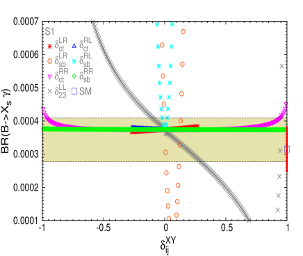
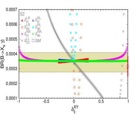
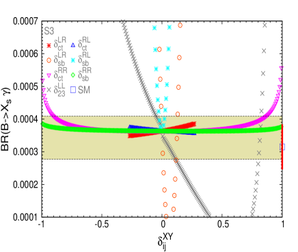
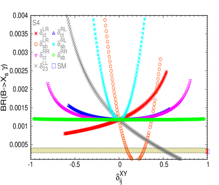
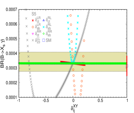
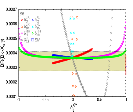
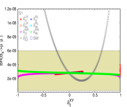
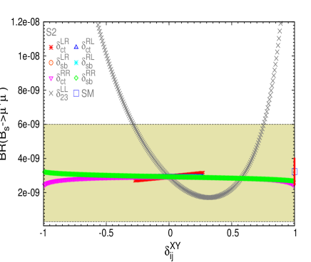
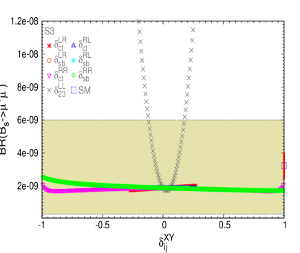
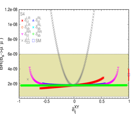
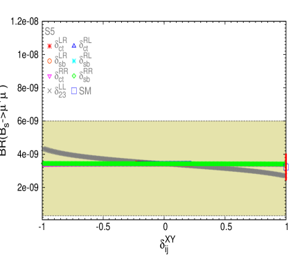
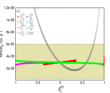
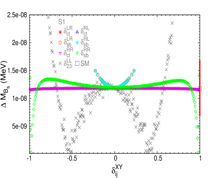
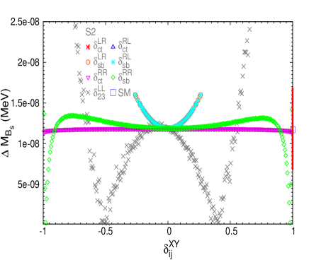
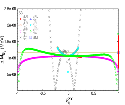
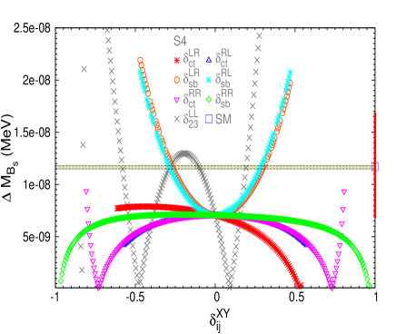
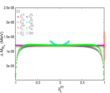
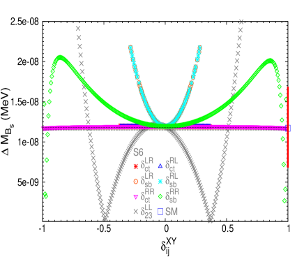
In Figs. 1 – 3 we show the results for the three flavor observables discussed in Sects. 3.2 – 3.4. The results are shown for the points S1…S6, see Tab. 1, where the various $\delta^{AB}_{ij}$ are varied individually. We have also included in the right vertical axis of these figures, for comparison, the respective SM prediction in Eqs. (31), (36), and (45). The red error bars displayed are the corresponding $3\,\sigma$ SM uncertainties (called $\Delta^{\rm theo}$). The shadowed horizontal bands in all cases, ${\rm BR}(B\to X_{s}\gamma)$ , ${\rm BR}(B_{s}\to\mu^{+}\mu^{-})$  and $\Delta M_{B_{s}}$, are their corresponding experimental measurements in Eqs. (30), (35) and (44), expanded with $3\,\sigma_{\rm exp}$ errors. In order to assess the total uncertainty the SM errors are also applied to the MSSM predictions. If this error bar is outside the experimental band the point can be regarded as excluded by the experimental measurement. It should be noted that the theory uncertainties can be larger in the MSSM than in the SM. However, estimates are much more complicated than in the SM and strongly dependent on the chosen SUSY parameters. Therefore we simply apply the SM uncertainty with $3\,\sigma$ errors.

Regarding the explored intervals for the deltas in the following Figs. 1 – 3, these will be $-1\leq\delta^{AB}_{ij}\leq 1$, as discussed above. However, in some cases these intervals are smaller: in computing the MSSM spectra with non-vanishing $\delta^{AB}_{ij}$ the code does not accept points that lead either to too low MSSM masses, excluded by experiment, or even non-physical negative squared masses. This is, for instance, the case of $\delta^{LR}_{ij}$ and $\delta^{RL}_{ij}$ with $ij=sb$ and $ij=ct$ that, as we can see in Figs. 1 – 3, are explored in smaller intervals since outside of them they lead to negative squared scalar masses. In particular, the contributions from the deltas leading to too low $M_{h}$ will be studied further in the following sections.

The analysis for ${\rm BR}(B\to X_{s}\gamma)$ is shown in Fig. 1 in the scenarios S1…S6. In the MFV case (i.e. for all $\delta^{AB}_{ij}=0$) we see that all points, except S4, are in agreement with experimental data. Only a very small variation with $\delta^{LR}_{ct}$, $\delta^{RL}_{ct}$, $\delta^{RR}_{ct}$, $\delta^{RR}_{sb}$ (except for S4) is observed. A clear dependence on $\delta^{LL}_{23}$ can be seen, placing bounds of ${\cal O}(0.1)$ on this NMFV parameter in all five scenarios, S1, S2, S3, S5 and S6. A very strong variation with $\delta^{LR}_{sb}$ and $\delta^{RL}_{sb}$ is found, which are restricted to very small values $\leq$ ${\cal O}(0.01)$ by the ${\rm BR}(B\to X_{s}\gamma)$ measurement. In scenario S4 the strong variation with $\delta^{LL}_{23}$ or $\delta^{LR}_{sb}$ can bring the prediction into agreement with the experimental data. Turning the argument around, the scenario S4, which appears to be excluded by the ${\rm BR}(B\to X_{s}\gamma)$ measurement is actually a valid scenario for certain values of $\delta^{LL}_{23}$ and $\delta^{LR}_{sb}$.

The results for ${\rm BR}(B_{s}\to\mu^{+}\mu^{-})$ are shown in Fig. 2 for the six scenarios. All $\delta^{AB}_{ij}$ show a relatively small impact, except for $\delta^{LL}_{23}$. From these plots we find the following allowed intervals for $\delta^{LL}_{23}$: $S1:(-0.3,0.7)$ , $S2:(-0.3,0.8)$, $S3:(-0.1,0.2)$, $S4:(-0.3,0.3)$, $S6:(-0.3,0.8)$. Therefore, bounds on this parameter ranging between $\sim-0.1$ and $\sim+0.8$ can be set in all scenarios except in S5 where we do not get any constraint. This scenario is characterized by a very large value of $M_{A}=1000\,\,\mathrm{GeV}$ and a relatively small value of $\tan\beta=10$, leading to a strong suppression of the contributions to ${\rm BR}(B_{s}\to\mu^{+}\mu^{-})$.

The predictions for $\Delta M_{B_{s}}$ in the six scenarios are shown in Fig. 3. While the experimental precision is very high the theoretical error is quite large, and the bounds on the $\delta^{AB}_{ij}$ are mainly given by the SM uncertainty in the $\Delta M_{B_{s}}$ prediction. All six scenarios for all $\delta^{AB}_{ij}=0$ are in agreement with the experimental data, once the SM uncertainty is taken into account. Except for S4, which is sensitive to all deltas, the other points are nearly insensitive to $\delta^{RR}_{ct}$, $\delta^{LR}_{ct}$ and $\delta^{RL}_{ct}$, therefore we do not get any additional bound for them in the allowed range from this observable. An important variation can be observed for $\delta^{LR}_{sb}$ and $\delta^{RL}_{sb}$. However, due to the MSSM particle mass restrictions commented above which shortened the allowed intervals, hardly any new bounds are placed by $\Delta M_{B_{s}}$, except in S4 and S6. Some sensitivity is found for $\delta^{RR}_{sb}$, especially in S4 and S6 where $|\delta^{RR}_{sb}|$ is bounded by $\leq{\cal O}(0.5)$. The strongest variation is found for $\delta^{LL}_{23}$, where due to the particular ’W-shape’ dependence, both intermediate and large values can be excluded.

The overall allowed intervals for the seven $\delta^{AB}_{ij}$ in the six scenarios and considering the three observables together, ${\rm BR}(B\to X_{s}\gamma)$, ${\rm BR}(B_{s}\to\mu^{+}\mu^{-})$and $\Delta M_{B_{s}}$, can be found in Tab. 2. From this table we then conclude on the strongest bounds that can be obtained from the combination of all three $B$-physics observables.

As a general comment, the main restrictions to the deltas come from ${\rm BR}(B\to X_{s}\gamma)$ and in some cases from $\Delta M_{B_{s}}$ and not yet from the young measurement ${\rm BR}(B_{s}\to\mu^{+}\mu^{-})$. The most restricted deltas are $\delta^{LR}_{sb}$ and $\delta^{RL}_{sb}$ that can reach values at most of ${\cal O}(0.01)$, then $\delta^{LL}_{23}$, $\delta^{LR}_{ct}$ and $\delta^{RL}_{ct}$ that can be at most of ${\cal O}(0.1)$, with the first one being slightly more restricted than the last two, and finally the less restricted deltas are $\delta^{RR}_{ct}$ and $\delta^{RR}_{sb}$ that in general can reach up to the largest explored values of ${\cal O}(1)$. Special attention deserves scenario S4, where, as mentioned above, setting $\delta^{AB}_{ij}=0$ leads to experimentally excluded predictions. Only non-zero values of $\delta^{LR}_{sb}$ can reconcile this scenario with experimental data. Consequently, assuming only one $\delta^{AB}_{ij}$ different from zero leads to an “excluded” scenario for all the other $\delta^{AB}_{ij}$ as shown in Tab. 2.

It can also be seen that larger constraints in the “$sb$ sector” than in the “$ct$ sector” are obtained, since the $B$-physics observables are in general more sensitive to mixing among $b$-type squarks. We also see that the $\delta^{LR}$ become more restricted than the others, since they involve the trilinear couplings that provide in general large corrections.

Regarding the comparison of our results with previous studies, we conclude that the bounds on the squark mixing deltas that we find here for the scenarios S1-S6 are more relaxed than in the set of benchmark scenarios that were analyzed in [5] before the LHC started operation. The scenarios investigated in the pre-LHC era contained relatively light scalar quarks (now excluded), leading to relatively large radiative corrections from NMFV effects. After the so far unsuccessful search for beyond SM physics at the LHC, scalar quark masses (in particular those of the first and second generation) have substantially higher lower bounds. Benchmark scenarios that take this into account (as our S1-S6) naturally permit larger values for the NMFV deltas.

		Total allowed intervals
$\delta^{LL}_{23}$	S1 S2 S3 S4 S5 S6	(-0.27:0.28) (-0.23:0.23) (-0.12:0.06) (0.17:0.19) excluded (-0.83:-0.78) (-0.14:0.14) (-0.076:0.14)
$\delta^{LR}_{ct}$	S1 S2 S3 S4 S5 S6	(-0.27:0.27) (-0.27:0.27) (-0.27:0.27) excluded (-0.22:0.22) (-0.37:0.37)
$\delta^{LR}_{sb}$	S1 S2 S3 S4 S5 S6	(-0.0069:0.014) (0.12:0.13) (-0.0069:0.014) (0.11:0.13) (-0.0069:0.014) (0.11:0.13) (0.076:0.12) (0.26:0.30) (-0.014:0.021) (0.17:0.19) (0:0.0069) (0.069:0.076)
$\delta^{RL}_{ct}$	S1 S2 S3 S4 S5 S6	(-0.27:0.27) (-0.27:0.27) (-0.27:0.27) excluded (-0.22:0.22) (-0.37:0.37)
$\delta^{RL}_{sb}$	S1 S2 S3 S4 S5 S6	(-0.034:0.034) (-0.034:0.034) (-0.034:0.034) excluded (-0.062:0.062) (-0.021:0.021)
$\delta^{RR}_{ct}$	S1 S2 S3 S4 S5 S6	(-0.99:0.99) (-0.99:0.99) (-0.98:0.97) excluded (-0.99:0.99) (-0.96:0.94)
$\delta^{RR}_{sb}$	S1 S2 S3 S4 S5 S6	(-0.96:0.96) (-0.96:0.96) (-0.96:0.94) excluded (-0.97:0.97) (-0.97:-0.94) (-0.63:0.64) (0.93:0.97)

Table 2: Present allowed intervals on the squark mixing parameters $\delta^{AB}_{ij}$ for the selected S1-S6 MSSM points defined in Tab. 1.

4.2 Framework 1: effects on Higgs boson masses

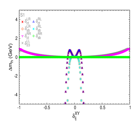
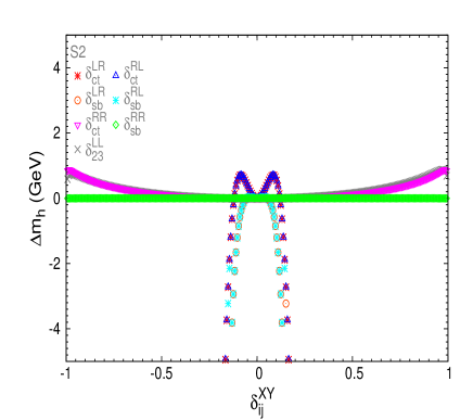
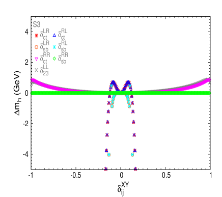
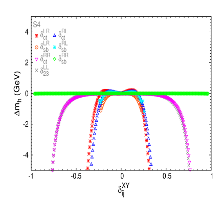
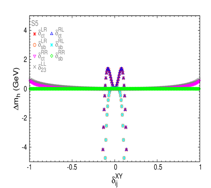
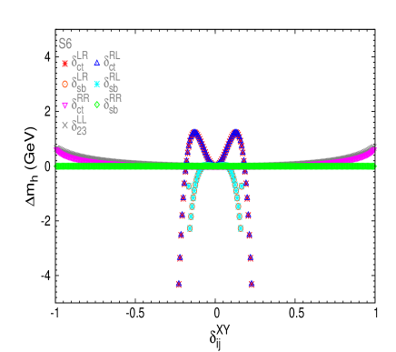
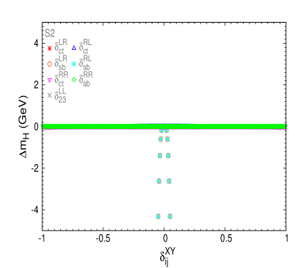
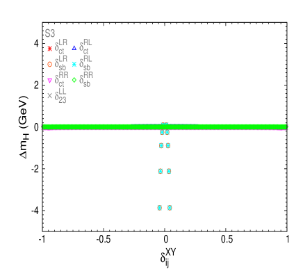
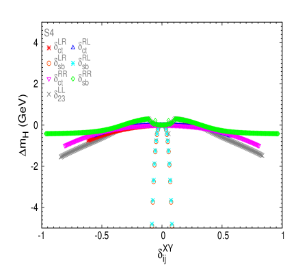
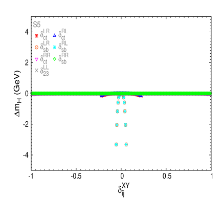
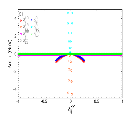
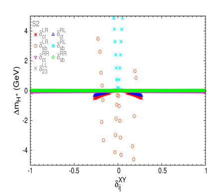
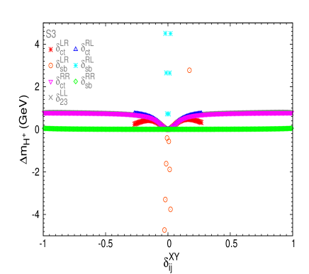
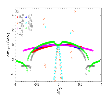
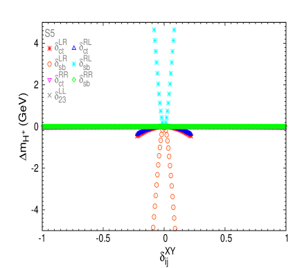
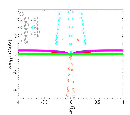
In this section we discuss the one-loop NMFV effects on the Higgs boson masses. A more detailed description of the computation of these one-loop NMFV effects in terms of one-loop diagrams and the corresponding corrections to the involved self-energies can be found in Ref. [5]. We are interested here mainly in the differences between the predictions within NMFV and MFV. We show, in Figs. 4, 5 and 6,

$$\Delta m_{\phi}:=M_{\phi}^{\rm NMFV}-M_{\phi}^{\rm MFV},\quad\phi=h,H,H^{\pm}$$ (46)

as a function of $\delta^{AB}_{ij}$ in the scenarios S1…S6.

We start our investigation with $\Delta m_{h}$ in Fig. 4. Bounds on the $\delta^{AB}_{ij}$ can in principle only be placed by the $M_{h}$ prediction, since this is the only mass parameter that has been measured experimentally so far. It should be noted that the value of $M_{h}^{\rm NMFV}$ depends strongly on the MFV SUSY parameters, in particular on $X_{t}$ (where $m_{t}X_{t}$ is the off-diagonal entry in the scalar top mass matrix). Consequently, delta values that produce an $M_{h}^{\rm NMFV}$ value slightly outside the allowed range, see Eqs. (23), (24), could be brought in agreement with experimental data by a small change in the scenario (e.g. by slightly changing the $X_{t}$ parameter).

As can be seen in Fig. 4, a negligible variation is found for $\delta^{RR}_{sb}$ in all scenarios. An enhancement of $M_{h}$ by up to $1\,\,\mathrm{GeV}$ is found for $\delta^{LL}_{23}$ and $\delta^{RR}_{ct}$ once the largest considered values of ${\cal O}(1)$ are reached. However, whereas these are possible for $\delta^{RR}_{ct}$, such large values are excluded in the $\delta^{LL}_{23}$ case, as we have seen in Tab. 2. The only exception here is scenario S4, where $\delta^{LL}_{23}$ and $\delta^{RR}_{ct}$ lead to a sizable reduction of $M_{h}$ once values larger than $\pm 0.5$ are reached. The remaining $\delta^{LR,RL}_{ij}$ have a larger impact on the $M_{h}$ prediction. Again the corresponding trilinear couplings involved play a relevant role here. Small $\delta^{LR,RL}_{ct}$ values lead to an enhancement of up to $1\,\,\mathrm{GeV}$, and larger values of ${\cal O}(0.1)$ yield a large negative contribution to $M_{h}$ (i.e. an effect similar to the dependence on $X_{t}$ can be observed). Consequently, bounds of ${\cal O}(0.2)$ can be placed on $\delta^{LR,RL}_{ct}$, predicting $M_{h}$ values that are outside the allowed range, see Eqs. (23), (24). Similar bounds can be derived for $\delta^{LR,RL}_{bs}$, however, these are in general weaker than the previous bounds found from the $B$-physics observables, as can be seen in Tab. 2. The strong sensitivity to $LR$ and $RL$ parameters can be understood due to the relevance of the ${\cal A}_{ij}$-terms in these Higgs mass corrections. It can be seen in the Feynman rules (i.e. see the coupling of two squarks and one/two Higgs bosons in Appendix A of Ref. [5]) that the ${\cal A}_{ij}$-terms enter directly into the couplings, and in some cases, as in the couplings of down-type squarks to the ${\cal CP}$-odd Higgs boson, enhanced by $\tan\beta$. Therefore, considering the relationship between the ${\cal A}_{ij}$-terms and these $LR$ and $RL$ parameters, as is shown in Eqs. (2), (7) and (8), the strong sensitivity to these parameters can be understood. A similar strong sensitivity to $\delta^{LR}_{ct}$ in $\Delta m_{h}$ has been found in [25].

The predictions for $\Delta m_{H}$ and $\Delta m_{H^{\pm}}$ are shown in Figs. 5 and 6. In general, only $\delta^{LR}_{sb}$ and $\delta^{RL}_{sb}$ lead to sizable effects in $M_{H}$ and $M_{H^{\pm}}$, where large (negative for $M_{H}$, and both negative and positive for $M_{H^{\pm}}$) contributions are found for delta values exceeding $\sim 0.05$. However, since these masses are mainly determined by the overall MSSM Higgs boson mass scale, $M_{A}$, no strong conclusions (or bounds stronger than from the $M_{h}$ prediction) can be drawn. On the other hand, these corrections will become relevant after a possible discovery of these heavy Higgs bosons.

Figure 4: One-loop corrections to $M_{h}$ in the scenarios S1…S6.

Figure 5: One-loop corrections to $M_{H}$ in the scenarios S1…S6.

Figure 6: One-loop corrections to $M_{H^{\pm}}$ in the scenarios S1…S6.

4.3 Framework 2:

The main goal of this part is to investigate how the upper bounds on the deltas can be placed from the corrections induced for the light MSSM Higgs boson mass. In order to explore the variation of these bounds for different choices in the MSSM parameter space, we investigate the four qualitatively different scenarios (a), (b), (c) and (d) defined in Eqs. (15), (16), (17) and (18), respectively. As explained above, the idea is to explore generic scenarios that are compatible with present data, in particular with the measurement of a Higgs boson mass, which we interpret as the mass of the light ${\cal CP}$-even Higgs boson in the MSSM (for all $\delta^{AB}_{ij}=0$), and the present experimental measurement of $(g-2)_{\mu}$. Taking these experimental results into account, we have re-analyzed the full set of bounds for the single deltas that are extracted from the requirement that the corrections to $M_{h}$ do not exceed $125.6\pm 5\,\,\mathrm{GeV}$  as a function of the two most relevant parameters in our framework 2: the generic SUSY mass scale $m_{\rm SUSY}$ $(\equiv m_{\rm SUSY-QCD})$ and $\tan\beta$. In order to find $M_{h}$ around $125.6\,\,\mathrm{GeV}$ for $\delta^{AB}_{ij}=0$ the scale $m_{\rm SUSY-QCD}$ as well as the trilinear couplings have been chosen to sufficiently high values, see Sect. 2.2.2. Alternatively one could choose scenarios with a light Higgs boson mass not in agreement with the experimental data and explore the regions of $\delta^{AB}_{ij}$ that reconcile the $M_{h}$ prediction with the experimental data. However, we will not pursue this alternative here.

We present the numerical results of our analysis in framework 2 in Fig. 7, where we restrict ourselves to the analysis of $\delta^{LR}_{ct}$ and $\delta^{RL}_{ct}$, which are the only parameters showing a strong impact on $M_{h}$, apart from $\delta^{LR}_{sb}$ and $\delta^{RL}_{sb}$ that are strongly restricted by $B$-physics observables, see the previous subsection. Furthermore, almost identical results are obtained for $\delta^{LR}_{ct}$ and $\delta^{RL}_{ct}$, and consequently, we restrict ourselves to one of those parameters. In each plot we show the resulting contourlines in the ($m_{\rm SUSY}$, $\tan\beta$) plane of maximum allowed value of $|\delta^{LR}_{ct}|$, i.e. the ones that do not lead to contributions to $M_{h}$ outside $125.6\pm 5\,\,\mathrm{GeV}$. The shaded areas in pink are the regions leading to a $(g-2)_{\mu}^{\rm SUSY}$ prediction, from the SUSY one-loop contributions, in the allowed interval of $(3.2,57.2)\times 10^{-10}$. The interior pink dashed contourline corresponds to $(g-2)_{\mu}^{\rm SUSY}$ exactly at the central value of the discrepancy $(g-2)_{\mu}^{\rm exp}-(g-2)_{\mu}^{\rm SM}=30.2\times 10^{-10}$. As in the previous framework 1, we use here again FeynHiggs [13, 14] to evaluate $M_{h}$ and SPHENO [46] to evaluate $(g-2)_{\mu}$ (where FeynHiggs gives very similar results). Due to the different relations between the SUSY-QCD and the SUSY-EW scales in our four scenarios the pink shaded areas differ substantially in the four plots. In particular in scenario (d), where we have set $m_{\rm SUSY-EW}:=m_{\rm SUSY-QCD}$ only relatively small values of $m_{\rm SUSY}$ yield a good prediction of $(g-2)_{\mu}^{\rm SUSY}$.

Figure 7: Contourlines in the ($m_{\rm SUSY}$, $\tan\beta$) plane of maximum squark mixing $|\delta^{LR}_{ct}|_{\rm max}$ that are allowed by the requirement that the correction to $M_{h}$ does not exceed $\pm 5\,\,\mathrm{GeV}$ for the scenarios (a), (b), (c) and (d) of our framework 2 The shaded (pink) areas are the regions leading to a $(g-2)_{\mu}^{\rm SUSY}$ prediction in the $(3.2,57.2)\times 10^{-10}$ interval. The interior pink dashed contourline corresponds to $(g-2)_{\mu}^{\rm SUSY}$ exactly at the central value of the discrepancy $(g-2)_{\mu}^{\rm exp}-(g-2)_{\mu}^{\rm SM}=30.2\times 10^{-10}$ .

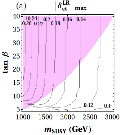
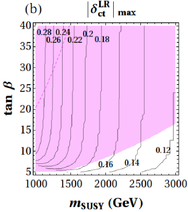
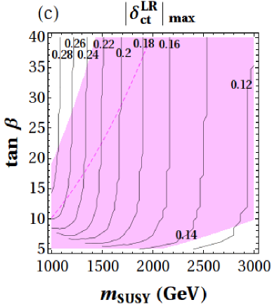
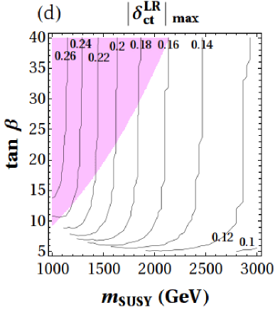
One can observe in Fig. 7 that the bounds on $|\delta^{LR}_{ct}|$ depend only weakly on the chosen scenario, such that they can be regarded as relatively general. For $m_{\rm SUSY}\sim 1\,\,\mathrm{TeV}$ bounds around $|\delta^{LR}_{ct}|\;\raisebox{-3.00003pt}{$\stackrel{{\scriptstyle\displaystyle<}}{{\sim}}$}\;0.28$ are found, whereas for $m_{\rm SUSY}\sim 3\,\,\mathrm{TeV}$ only $|\delta^{LR}_{ct}|\;\raisebox{-3.00003pt}{$\stackrel{{\scriptstyle\displaystyle<}}{{\sim}}$}\;0.12$ is allowed. For most of the parameter space the results are nearly independent of $\tan\beta$. Only for $\tan\beta\;\raisebox{-3.00003pt}{$\stackrel{{\scriptstyle\displaystyle<}}{{\sim}}$}\;7$ smaller bounds for smaller $m_{\rm SUSY}$ values are reached. The results are consistent with previous findings, i.e. large SUSY mass scales, leading to larger intergenerational mixing terms (and in particular $A$-terms) lead to larger effects and thus to smaller allowed $\delta^{AB}_{ij}$. Comparing the obtained contours, which depend on $m_{\rm SUSY-QCD}$, with the $(g-2)_{\mu}$ preferred regions, which depend on $m_{\rm SUSY-EW}$, slightly smaller $|\delta^{LR}_{ct}|_{\rm max}$ values as in (c) or slightly larger ones as in (d) are favored. However, this just reflects the choice of the hierarchy between these two fundamental mass scales used in the respective scenario.

5 Conclusions

We presented an up-to-date comparison of the predictions for flavor and Higgs observables based on NMFV parameters in the MSSM with the current experimental data. The flavor observables include ${\rm BR}(B\to X_{s}\gamma)$, ${\rm BR}(B_{s}\to\mu^{+}\mu^{-})$ and $\Delta M_{B_{s}}$. In the Higgs sector we evaluated the corrections to the light and heavy ${\cal CP}$-even Higgs masses as well as to the charged Higgs boson mass. Within the MSSM the calculations were performed at the full one-loop level with the full (s)quark flavor structure, i.e. not relying on the mass insertion or other approximations.

In the first part we analyzed six representative scenarios which are in agreement with current bounds on the SUSY and Higgs searches at the LHC. We derived the most up-to-date bounds on $\delta^{AB}_{ij}$ within these six scenarios from flavor observables, thus giving an idea of the overall size of these parameters taking the latest experimental bounds into account. The corresponding contributions indicate which level of higher-order corrections are possible and allowed by the inclusion of NMFV. In particular in the case of the light Higgs boson we find that the prediction of $M_{h}$ can lead to additional new constraints on the deltas, specifically on $\delta^{LR}_{ct}$ and $\delta^{RL}_{ct}$. This is due to the fact that ${\cal A}_{ij}$-terms enter directly into the couplings, creating a strong sensitivity to these parameters.

In the second part we analyzed four different two-dimensional scenarios, which are characterized by universal scales for the SUSY electroweak scale, $m_{\rm SUSY-EW}$, that determines the masses of the scalar leptons and electroweak particles, and for the SUSY QCD scale, $m_{\rm SUSY-QCD}$, that determines the masses of the scalar quarks. As additional free parameter we kept $\tan\beta$. Within this simplified model it is possible to analyze the behavior of the corrections to $M_{h}$, where at the same time agreement with the anomalous magnetic moment of the muon, $(g-2)_{\mu}$ is required. We demanded that the correction to $M_{h}$ does not yield values outside $125.6\pm 5\,\,\mathrm{GeV}$, leading to new improved bounds on $\delta^{LR}_{ct}$ and $\delta^{RL}_{ct}$, whereas no limits on the other $\delta^{AB}_{ij}$can be obtained. The limits on $|\delta^{LR}_{ct}|$ turn out to be relatively independent on the choice of the scenario. For $m_{\rm SUSY-QCD}\sim 1(3)\,\,\mathrm{TeV}$ bounds of $|\delta^{LR}_{ct}|\;\raisebox{-3.00003pt}{$\stackrel{{\scriptstyle\displaystyle<}}{{\sim}}$}\;0.28(0.12)$ were found. These bounds on $\delta^{LR}_{ct}$ and $\delta^{RL}_{ct}$ are genuine from Higgs physics and do not have competitive bounds from $B$-physics observables.

Acknowledgments

The work of S.H. was supported by the Spanish MICINN’s Consolider-Ingenio 2010 Program under grant MultiDark CSD2009-00064. The work of M.H. and M.A.-C. was partially supported by the European Union FP7 ITN INVISIBLES (Marie Curie Actions, PITN- GA-2011- 289442), by the CICYT through the project FPA2012-31880, by the Spanish Consolider-Ingenio 2010 Programme CPAN (CSD2007-00042) and by the Spanish MINECO’s “Centro de Excelencia Severo Ocho” Programme under grant SEV-2012-0249.