Power Scaling of Uplink Massive MIMO Systems with Arbitrary-Rank Channel Means

Abstract

This paper investigates the uplink achievable rates of massive multiple-input multiple-output (MIMO) antenna systems in Ricean fading channels, using maximal-ratio combining (MRC) and zero-forcing (ZF) receivers, assuming perfect and imperfect channel state information (CSI). In contrast to previous relevant works, the fast fading MIMO channel matrix is assumed to have an arbitrary-rank deterministic component as well as a Rayleigh-distributed random component. We derive tractable expressions for the achievable uplink rate in the large-antenna limit, along with approximating results that hold for any finite number of antennas. Based on these analytical results, we obtain the scaling law that the users’ transmit power should satisfy, while maintaining a desirable quality of service. In particular, it is found that regardless of the Ricean $K$-factor, in the case of perfect CSI, the approximations converge to the same constant value as the exact results, as the number of base station antennas, $M$, grows large, while the transmit power of each user can be scaled down proportionally to $1/M$. If CSI is estimated with uncertainty, the same result holds true but only when the Ricean $K$-factor is non-zero. Otherwise, if the channel experiences Rayleigh fading, we can only cut the transmit power of each user proportionally to $1/\sqrt{M}$. In addition, we show that with an increasing Ricean $K$-factor, the uplink rates will converge to fixed values for both MRC and ZF receivers.

I Introduction

Multiple-input multiple-output (MIMO) antenna technology has emerged as an effective technique for significantly improving the capacity of wireless communication systems [1, 2]. Recently, multiuser MIMO (MU-MIMO) systems, where a base station (BS) equipped with multiple antennas serves a number of users in the same time-frequency resource, have gained much attention because of their considerable spatial multiplexing gains even without multiple antennas at the users [3, 4, 5, 6]. To reap all the benefits of MIMO at a greater scale, the paradigm of massive MIMO, which considers the use of hundreds of antenna elements to serve tens of users simultaneously, has recently come at the forefront of wireless communications research [7].

Great efforts have been made to understand the spectral and energy efficiency gains of massive MIMO systems, e.g., [8, 9, 10, 11, 12, 7, 13, 14]. In particular, [8] indicates that the high number of degrees-of-freedom can average out the effects of fast fading. It has further been revealed in [10] that, when the number of antennas increases without bound, uncorrelated noise, fast fading and intracell interference vanish. The only impairment left is pilot-contamination. Another merit of massive MIMO is that the transmit power can be greatly reduced. In [12], the power-scaling law was investigated and it was shown that, as the number of BS antennas grows without limit, the uplink rate can be maintained while the transmit power can be substantially cut down. For example, ideally, to maintain the same quality-of-service as with a single-antenna BS, the transmit power of a 100-antenna BS would be only almost $1\%$ of the power of the single-antenna one.

The increasing physical size of massive MIMO arrays is a fundamental problem for practical deployment and utilization and the millimeter-wave operating from $30-300$ GHz finds a way out, since the small wavelengths make possible for many antenna elements to be packed with a finite volume. On top of this, due to the highly directional and quasi-optical nature of propagation at millimeter-waves, line-of-sight (LOS) propagation is dominating [15, 16, 17]. Therefore, massive MIMO systems operating in LOS conditions is expected to be a novel paradigm. Unfortunately, many of the existing pioneering works simply assume Rayleigh fading conditions [8, 10, 12]. While this assumption simplifies extensively all mathematical manipulations, it falls short of capturing the fading variations when there is a specular or LOS component between the transmitter and receiver. As such, more general fading models need to be considered.

In this paper, we extend the results in [12] to Ricean fading channels with arbitrary-rank mean matrices. In [12], the authors studied the potential of power savings in massive MU-MIMO systems, assuming that the fast fading channel matrix has zero-mean unit-variance entries. In our analysis, the fast fading channel matrix consists of an arbitrary-rank deterministic component, and a Rayleigh-distributed random component accounting for the scattered signals [18]. We consider a single-cell MU-MIMO system in the uplink, where both maximal-ratio combining (MRC) and zero-forcing (ZF) receivers are assumed at the BS, with perfect and imperfect channel state information (CSI). Some relevant works on Ricean fading in massive MIMO systems are [19, 20, 21, 22]. However, [19] considers the single-user scenario and in [20, 21, 22], the numbers of antennas at the transmitters and the receiver go to infinity with a constant ratio. Our main contributions include new, tractable expressions for the achievable uplink rate in the large-antenna limit, along with approximating results that hold for any finite number of antennas. We also elaborate on the power-scaling laws as follows:

• We reveal that under Ricean fading, with perfect CSI, if the number of BS antennas, $M$, grows asymptotically large, we can cut down the transmit power of each user proportionally to $1/M$ to maintain a desirable rate. In addition, as $M\to\infty$, the sum rates of both MRC and ZF receivers converge to the same constant value, indicating that in the large-system limit, intracell interference disappears.

• If CSI is estimated with uncertainty, then when $M$ gets asymptotically large, massive MIMO will still bring considerate power savings for each user. In particular, if the Ricean $K$-factor is non-zero, the transmit power for each user can be scaled down by $1/M$ to obtain the same rate, while the uplink rates will tend to a fixed value as a function of Ricean $K$-factor. However, when the Ricean $K$-factor is zero, the transmit power can be scaled down only by $1/{\sqrt{M}}$ and the uplink rates will again approach to a fixed value if $M\to\infty$.

The remainder of the paper is organized as follows. Section II describes the MU-MIMO system model in Ricean fading channels, and provides the definition of the uplink rate with perfect and imperfect CSI. Section III derives closed-form approximations for the achievable uplink rates and also investigates the power-scaling laws. In Section IV, we provide a set of numerical results, while Section V summarizes the main results of this paper.

Notation—Throughout the paper, vectors are expressed in lowercase boldface letters while matrices are denoted by uppercase boldface letters. We use ${{\bf{X}}^{H}},{{\bf{X}}^{T}},{\bf{X}^{*}}$ and $\mathbf{X}^{-1}$ to denote the conjugate-transpose, transpose, conjugate and inverse of $\bf{X}$, respectively. Moreover, $\mathbf{I}_{N}$ denotes an $N\times N$ identity matrix, $\delta_{ni}$ equals $1$ when $n=i$ and $0$ otherwise, and $[{\bf{X}}]_{ij}$ or ${\bf{X}}_{ij}$ gives the ($i,j$)th entry of $\bf{X}$. Finally, $\mathbb{E}\left\{\cdot\right\}$ is the expectation operator, $\left\|{\,\cdot\,}\right\|$ is the Euclidean norm and $\mathbf{Z}\sim{\cal CN}\left(\mathbf{A},\mathbf{B}\right)$ denotes that $\mathbf{Z}$ is a complex Gaussian matrix with mean matrix $\mathbf{A}$ and covariance matrix $\mathbf{B}$.

II System Model

We consider a MU-MIMO system with $N$ single-antenna users and an $M$-antenna BS, where users transmit their signals to the BS in the same time-frequency channel. The system is single-cell with no interference from neighboring cells. The received vector ${\mathbf{y}}\in{{\mathbb{C}}^{M\times 1}}$ at the BS can be written as [11]

$${\mathbf{y}}=\sqrt{{p_{u}}}{\mathbf{Gx}}+{\mathbf{n}},$$ (1)

where $\mathbf{G}$ denotes the $M\times N$ MIMO channel matrix between the BS and the $N$ users, $\sqrt{p_{u}}\mathbf{x}$ denotes the $N\times 1$ vector containing the transmitted signals from all users, $p_{u}$ is the average transmitted power of each user, and $\mathbf{n}$ represents the vector of zero-mean additive white Gaussian noise (AWGN). To facilitate our analysis and without loss of generality, the noise variance is assumed to be $1$.

II-A Channel Model

We denote the channel coefficient between the $n$th user and the $m$th antenna of the BS as ${g_{mn}}={[\mathbf{G}]_{mn}}$, which embraces independent fast fading, geometric attenuation and log-normal shadow fading [10] and can be expressed as

$${g_{mn}}={h_{mn}}\sqrt{{\beta_{n}}},$$ (2)

where $h_{mn}$ is the fast fading element from the $n$th user to the $m$th antenna of the BS, while $\beta_{n}$ is the large-scale fading coefficient to model both the geometric attenuation and shadow fading, which is assumed to be constant across the antenna array. Under this model, we can write

$${\mathbf{G}}={\mathbf{H}}{{\mathbf{D}}^{1/2}},$$ (3)

where $\mathbf{H}$ denotes the $M\times N$ channel matrix modeling fast fading between the users and the BS, i.e., ${[\mathbf{H}]_{mn}}={h_{mn}}$ and $\mathbf{D}$ is the $N\times N$ diagonal matrix with ${[\mathbf{D}]_{nn}}={\beta_{n}}$. The fast fading matrix consists of two parts, namely a deterministic component corresponding to the LOS signal and a Rayleigh-distributed random component which accounts for the scattered signals. Moreover, the Ricean factor, represents the ratio of the power of the deterministic component to the power of the scattered components. Here, we assume that the Ricean $K$-factor of each user is different and the $n$th user’s $K$-factor is denoted by $K_{n}$. Then, the fast fading matrix $\mathbf{H}$ can be written as [23]

$${\mathbf{H}}={\mathbf{\bar{H}}}{\left[{\boldsymbol{\Omega}{{\left({\boldsymbol{\Omega}+\mathbf{I}_{N}}\right)}^{-1}}}\right]^{1/2}}+{{\mathbf{H}}_{w}}{\left[{{{\left({\boldsymbol{\Omega}+\mathbf{I}_{N}}\right)}^{-1}}}\right]^{1/2}},$$ (4)

where $\boldsymbol{\Omega}$ is a $N\times N$ diagonal matrix with $\left[\boldsymbol{\Omega}\right]_{nn}=K_{n}$, ${\mathbf{H}_{w}}$ denotes the random component, the entries of which are independent and identically distributed (i.i.d.) Gaussian random variables with zero-mean, independent real and imaginary parts, each with variance $1/2$, and $\mathbf{\bar{H}}$ denotes the deterministic component, which was usually assumed to be rank-$1$ in previous studies, e.g., [18, 24, 25, 19]. In this paper, due to the assumption of multiple geographically distributed users, this constraint is relaxed and we let $\mathbf{\bar{H}}$ have an arbitrary rank as [26]

$${\left[{\mathbf{\bar{H}}}\right]_{mn}}={e^{-j(m-1)\frac{{2\pi d}}{\lambda}{\sin\left(\theta_{n}\right)}}},$$ (5)

where $d$ is the antenna spacing, $\lambda$ is the wavelength, and $\theta_{i}$ is the arrival angle of the $i$th user. For convenience, we will set $d=\lambda/2$ in the rest of this paper.

II-B Achievable Uplink Rate

II-B1 Perfect CSI

We first consider the case that the BS has perfect CSI. Let $\mathbf{A}$ be the $M\times N$ linear receiver matrix which depends on the channel matrix $\mathbf{G}$. The BS processes its received signal vector by multiplying it with the conjugate-transpose of the linear receiver as [10]

$${\mathbf{r}}=\mathbf{A}^{H}\mathbf{y}.$$ (6)

Then, substituting (1) into (6) gives

$${\mathbf{r}}=\sqrt{{p_{u}}}{\mathbf{A}^{H}}\mathbf{Gx}+{\mathbf{A}^{H}}\mathbf{n}.$$ (7)

The $n$th element of $\mathbf{r}$ can be written as

$${r_{n}}=\sqrt{{p_{u}}}\mathbf{a}_{n}^{H}\mathbf{Gx}+\mathbf{a}_{n}^{H}\mathbf{n},$$ (8)

where $\mathbf{a}_{n}$ is the $n$th column of $\mathbf{A}$. By the law of matrix multiplication, we further get

$${r_{n}}=\sqrt{{p_{u}}}\mathbf{a}_{n}^{H}{\mathbf{g}_{n}}{x_{n}}+\sqrt{{p_{u}}}\sum_{i=1\atop i\neq n}^{N}{\mathbf{a}_{n}^{H}{\mathbf{g}_{i}}{x_{i}}}+\mathbf{a}_{n}^{H}\mathbf{n},$$ (9)

where $x_{n}$ denotes the $n$th element of $\mathbf{x}$ and $\mathbf{g}_{n}$ is the $n$th column of $\mathbf{G}$. Assuming an ergodic channel, the achievable uplink rate of the $n$th user is given by [12]

$${R_{{\sf P},n}}=\mathbb{E}\left\{{{{\log}_{2}}\left({1+\frac{{{p_{u}}{{\left|{\mathbf{a}_{n}^{H}{\mathbf{g}_{n}}}\right|}^{2}}}}{{{p_{u}}\sum_{i=1\atop i\neq n}^{N}{{{\left|{\mathbf{a}_{n}^{H}{\mathbf{g}_{i}}}\right|}^{2}}}+{{\left\|{{\mathbf{a}_{n}}}\right\|}^{2}}}}}\right)}\right\}.$$ (10)

Therefore, the uplink sum rate per cell, measured in bits/s/Hz, can be defined as

$$C_{\sf P}=\sum\limits_{n=1}^{N}{{R_{\sf{P},n}}}.$$ (11)

II-B2 Imperfect CSI

In real situations, the channel matrix $\mathbf{G}$ is estimated at the BS. For the considered Ricean fading channel model, we assume that both the deterministic LOS component and the Ricean $K$-factor matrix $\boldsymbol{\Omega}$ are perfectly known at both the transmitter and receiver, such that the estimate of $\mathbf{G}$ can be expressed as

$${\bf{\hat{G}}}={\bf{\bar{G}}}{\left[{\boldsymbol{\Omega}{{\left({\boldsymbol{\Omega}+\mathbf{I}_{N}}\right)}^{-1}}}\right]^{1/2}}+{{\bf{\hat{G}}}_{w}}{\left[{{{\left({\boldsymbol{\Omega}+\mathbf{I}_{N}}\right)}^{-1}}}\right]^{1/2}},$$ (12)

where ${\bf{\bar{G}}}$ denotes the deterministic component of $\mathbf{G}$, i.e., ${\bf{\bar{G}}}\triangleq{\bf{\bar{H}}}{{\bf{D}}^{1/2}}$ and ${{\bf{\hat{G}}}_{w}}$ represents the estimate of the random component $\mathbf{G}_{w}\triangleq\mathbf{H}_{w}\mathbf{D}^{1/2}$. In this paper, we consider that the channel is estimated using uplink pilots. Let an interval of length $\tau$ symbols be used for uplink training, where $\tau$ is smaller than the coherence time of the channel. In the training stage, all users simultaneously transmit orthogonal pilot sequences of $\tau$ symbols, which can be stacked into a $\tau\times N$ matrix $\sqrt{p}_{p}\boldsymbol{\Phi}$ $\left(\tau\geq N\right)$, which satisfies $\mathbf{F}^{H}\mathbf{F}=\mathbf{I}_{N}$, where $\mathbf{F}\triangleq\boldsymbol{\Phi}\left[\left(\boldsymbol{\Omega}+\mathbf{I}_{N}\right)^{-1}\right]^{1/2}$ and $p_{p}=\tau p_{u}$ is the transmit pilot power. As a result, the BS receives the $M\times\tau$ noisy pilot matrix as

$${\mathbf{Y}_{p}}=\sqrt{{p_{p}}}\mathbf{G}{\boldsymbol{\Phi}^{T}}+\mathbf{N},$$ (13)

where $\mathbf{N}$ represents the $M\times\tau$ AWGN matrix with i.i.d. zero-mean and unit-variance elements. With (4), we can remove the LOS component, which is assumed to be already known from (13), and the remaining terms of the received matrix are

$$\mathbf{Y}_{p,w}=\sqrt{{p_{p}}}\mathbf{G}_{w}{\left[{{{\left({\boldsymbol{\Omega}+\mathbf{I}_{N}}\right)}^{-1}}}\right]^{1/2}}{\boldsymbol{\Phi}^{T}}+\mathbf{N},$$ (14)

which can be further written as

$$\mathbf{Y}_{p,w}=\sqrt{{p_{p}}}\mathbf{G}_{w}\mathbf{F}^{T}+\mathbf{N}.$$ (15)

The minimum mean-square-error (MMSE) estimate of ${{\bf{\hat{G}}}_{w}}$ from $\mathbf{Y}_{p,w}$ is [28]

$${{\bf{\hat{G}}}_{w}}=\frac{1}{{\sqrt{{p_{p}}}}}{\mathbf{Y}_{p}}{\mathbf{F}^{*}}{\bf{\tilde{D}}},$$ (16)

where ${\bf{\tilde{D}}}\triangleq{\left({\frac{1}{{{p_{p}}}}{{\bf{D}}^{-1}}+{{\bf{I}}_{N}}}\right)^{-1}}$. From (13), we can easily get

$${{\bf{\hat{G}}}_{w}}=\left({{{\bf{G}}_{w}}+\frac{1}{{\sqrt{{p_{p}}}}}{\bf{W}}}\right){\bf{\tilde{D}}},$$ (17)

where $\bf{W}\triangleq\bf{N}\mathbf{F}^{*}$. Noting that $\mathbf{F}^{H}\mathbf{F}={\bf I}_{N}$, the entries of $\bf W$ are i.i.d. Gaussian random variables with zero-mean and unit-variance. Let $\boldsymbol{\Xi}\triangleq\bf{\hat{G}}-\bf G$ denote the channel estimation error and $\mathbf{\hat{A}}$ be the linear receiver matrix which depends on $\mathbf{\hat{G}}$. Then, after linear reception, we have

$${\mathbf{\hat{r}}}=\sqrt{{p_{u}}}{\mathbf{\hat{A}}^{H}}\left(\mathbf{\hat{G}x}-\boldsymbol{\Xi x}\right)+{\mathbf{\hat{A}}^{H}}\mathbf{n}.$$ (18)

As such, the estimated signal for the $n$th user is given by

$${\hat{r}_{n}}=\sqrt{{p_{u}}}\mathbf{\hat{a}}_{n}^{H}\mathbf{\hat{G}x}-\sqrt{{p_{u}}}\mathbf{\hat{a}}_{n}^{H}\boldsymbol{\Xi}\mathbf{x}+\mathbf{\hat{a}}_{n}^{H}\mathbf{n},$$ (19)

where $\mathbf{\hat{a}}_{n}$ is the $n$th column of $\mathbf{\hat{A}}$, and (19) can be easily rewritten as

$${\hat{r}_{n}}\negthickspace=\negthickspace\sqrt{{p_{u}}}\mathbf{\hat{a}}_{n}^{H}{\mathbf{\hat{g}}_{n}}{x_{n}}+\sqrt{{p_{u}}}\negthickspace\sum_{i=1\atop i\neq n}^{N}{\mathbf{\hat{a}}_{n}^{H}{\mathbf{\hat{g}}_{i}}{x_{i}}}-\sqrt{p_{u}}\negthickspace\sum_{i=1}^{N}{\mathbf{\hat{a}}_{n}^{H}\boldsymbol{\xi_{i}}\mathbf{x_{i}}}+\mathbf{\hat{a}}_{n}^{H}\mathbf{n},$$ (20)

where $\mathbf{\hat{g}}_{i}$ and $\boldsymbol{\xi}_{i}$ are the $i$th columns of $\mathbf{\hat{G}}$ and $\boldsymbol{\Xi}$, respectively. Note that the last three terms in (20) correspond to intracell interference, channel estimation error and noise, respectively. According to the classical assumption of worst-case uncorrelated Gaussian noise [12], along with the fact that the variance of elements of estimation error vector $\boldsymbol{\xi}_{i}$ is

$$\mathbb{E}\left\{{\left|\right.}{\left[\boldsymbol{\Xi}\right]_{mi}}-\mathbb{E}\left\{\left[\boldsymbol{\Xi}\right]_{mi}\right\}{\left.\right|}^{2}\right\}={\frac{{{\beta_{i}}}}{{\left({1+{p_{p}}{\beta_{i}}}\right)\left({K_{i}+1}\right)}}},$$ (21)

the achievable uplink rate of the $n$th user can be given by (22) (at the top of the next page).

$${R_{{\sf IP},n}}=\mathbb{E}\left\{{{{\log}_{2}}\left({1+\frac{{{p_{u}}{{\left|{{\bf{\hat{a}}}_{n}^{H}{{{\bf{\hat{g}}}}_{n}}}\right|}^{2}}}}{{{p_{u}}\sum_{i=1\atop i\neq n}^{N}{{{\left|{{\bf{\hat{a}}}_{n}^{H}{{{\bf{\hat{g}}}}_{i}}}\right|}^{2}}}+\sum_{i=1}^{N}{{{\left\|{\bf{\hat{a}}}_{n}\right\|^{2}{\frac{{{p_{u}\beta_{i}}}}{{\left({1+{p_{p}}{\beta_{i}}}\right)\left({K_{i}+1}\right)}}}}}+}{{\left\|{{{{\bf{\hat{a}}}}_{n}}}\right\|}^{2}}}}}\right)}\right\}.$$ (22)

Similar to the perfect CSI case, the uplink sum rate per cell can be defined as

$$C_{\sf IP}=\frac{T-\tau}{T}\sum_{n=1}^{N}{{R_{\sf{IP},n}}},$$ (23)

where $T$ represents the coherence time of the channel, in terms of the number of symbols, during which $\tau$ $(\tau\leq T)$ symbols are used as pilots for channel estimation.

III Analysis of Achievable Uplink Rate

In this section, we derive closed-form expressions for the achievable uplink rates in the large-antenna limit along with tractable approximations that hold for any finite number of antennas. Note that our results are tight and apply for systems with arbitrary-rank Ricean fading channel mean matrices. We also quantify the power-scaling laws in the cases of perfect and imperfect CSI. A key preliminary result is given first.

Lemma 1

If $X=\sum_{i=1}^{t_{1}}{X_{i}}$ and $Y=\sum_{j=1}^{t_{2}}{Y_{j}}$ are both sums of nonnegative random variables $X_{i}$ and $Y_{j}$, then we get the following approximation

$$\mathbb{E}\left\{\log_{2}\left(1+\frac{X}{Y}\right)\right\}\approx\log_{2}\left(1+\frac{\mathbb{E}\left\{X\right\}}{\mathbb{E}\left\{Y\right\}}\right),$$ (24)

Proof:

See Appendix A. ∎

Note that the approximation in (24) does not require the random variables $X$ and $Y$ to be independent and becomes more accurate as $t_{1}$ and $t_{2}$ increase. Thus, in massive MIMO systems, due to the large number of BS antennas, this approximation will be particularly accurate.

III-A Perfect CSI

We begin by considering the case with perfect CSI and establishing some key preliminary results which will be useful in deriving our main results.

Lemma 2

By the law of large numbers, when $M$ is asymptotically large, we have

$$\frac{1}{M}\mathbf{H}^{H}\mathbf{H}\xrightarrow{a.s.}\mathbf{I}_{N},$$ (25)

where –a.s. denotes almost sure convergence.

Proof:

See Appendix B. ∎

Lemma 3

The expectation for the inner product of two same columns in $\mathbf{H}$ can be found as

$$\mathbb{E}{\left\{\left\|{{{\mathbf{h}}_{n}}}\right\|^{2}\right\}}=\mathbb{E}\left\{{\bf h}_{n}^{H}{\bf h}_{n}\right\}=M,$$ (26)

and the expectation of the norm-square of the inner product of any two columns in $\mathbf{H}$ is given by

$$\mathbb{E}{\left\{\left|{{\mathbf{h}}_{n}^{H}{{\mathbf{h}}_{i}}}\right|^{2}\right\}}\negthickspace=\negthickspace {\frac{{2MK_{n}\negthickspace+\negthickspace M}}{{{{(K_{n}\negthickspace+\negthickspace 1)}^{2}}}}\negthickspace+\negthickspace{M^{2}}},\negthickspace\negthickspace\negthickspace i=n$$ , (27)

$$\mathbb{E}{\left\{\left|{{\mathbf{h}}_{n}^{H}{{\mathbf{h}}_{i}}}\right|^{2}\right\}}\negthickspace=\negthickspace \frac{{{K_{n}K_{i}}{\phi^{2}_{ni}}\negthickspace+\negthickspace M\left(K_{n}\negthickspace+\negthickspace K_{i}\right)\negthickspace+\negthickspace M}}{{{{(K_{n}\negthickspace+\negthickspace 1)(K_{i}\negthickspace+\negthickspace 1)}}}},\negthickspace\negthickspace\negthickspace i\neq n$$ , (28)

where $\phi_{ni}$ is defined as

$$\phi_{ni}\triangleq\frac{{\sin\left({\frac{M\pi}{2}\left[{\sin\left({\theta_{n}}\right)-\sin\left({\theta_{i}}\right)}\right]}\right)}}{{{\sin\left({\frac{\pi}{2}\left[{\sin\left({\theta_{n}}\right)-\sin\left({\theta_{i}}\right)}\right]}\right)}}}.$$ (29)

Proof:

See Appendix C. ∎

III-A1 MRC Receivers

For MRC, the linear receiver matrix is given by

$$\mathbf{A}=\mathbf{G},$$ (30)

which yields $\mathbf{a}_{n}=\mathbf{g}_{n}$. From (10), the achievable rate of the $n$th user is

$${R_{{\sf P},n}^{\sf mrc}}=\mathbb{E}\left\{{{{\log}_{2}}\left({1+\frac{{{p_{u}}{{\left\|{{\mathbf{g}_{n}}}\right\|}^{4}}}}{{{p_{u}}\sum_{i=1\atop i\neq n}^{N}{{{\left|{\mathbf{g}_{n}^{H}{\mathbf{g}_{i}}}\right|}^{2}}}+{{\left\|{{\mathbf{g}_{n}}}\right\|}^{2}}}}}\right)}\right\}.$$ (31)

Next, we will investigate the power-scaling properties of the uplink rate in (31); this is done by first presenting the exact rate limit in the theorem below.

Theorem 1

Using MRC receivers with perfect CSI, if the transmit power of each user is scaled down by a factor of ${1}/{M^{\alpha}}$, i.e., $p_{u}={E_{u}}/{M^{\alpha}}$ for $\alpha>0$ and a fixed $E_{u}$, we have

$$R_{{\sf P},n}^{\sf mrc}-\accentset{\mbox{\large.}}{R}_{{\sf P},n}^{\sf mrc}\to 0,~{}\mbox{as }M\to\infty,$$ (32)

where $\accentset{\mbox{\large.}}{R}_{{\sf P},n}^{\sf mrc}\triangleq{\log_{2}}\left({1+\frac{{{E_{u}}{\beta_{n}}}}{{{M^{\alpha-1}}}}}\right)$.

Proof:

Let $p_{u}={E_{u}}/{M^{\alpha}}$, where $\alpha>0$. Substituting it into (31), we obtain

$$R_{{\sf P},n}^{\sf mrc}=\mathbb{E}\left\{{{{\log}_{2}}\left({1+\frac{{\frac{{{E_{u}}}}{M^{\alpha}}{{\left\|{{{\bf{g}}_{n}}}\right\|}^{4}}}}{{\frac{{{E_{u}}}}{M^{\alpha}}\sum_{i=1\atop i\neq n}^{N}{{{\left|{{\bf{g}}_{n}^{H}{{\bf{g}}_{i}}}\right|}^{2}}}+{{\left\|{{{\bf{g}}_{n}}}\right\|}^{2}}}}}\right)}\right\}.$$ (33)

We can also get

$$R_{{\sf P},n}^{\sf mrc}=\mathbb{E}\left\{{{{\log}_{2}}\left({1+\frac{{\frac{{{E_{u}}}}{M^{\alpha}}\frac{1}{M^{2}}{{\left\|{{{\bf{g}}_{n}}}\right\|}^{4}}}}{{\frac{{{E_{u}}}}{M^{\alpha}}\frac{1}{M^{2}}\sum_{i=1\atop i\neq n}^{N}{{{\left|{{\bf{g}}_{n}^{H}{{\bf{g}}_{i}}}\right|}^{2}}}+\frac{1}{M^{2}}{{\left\|{{{\bf{g}}_{n}}}\right\|}^{2}}}}}\right)}\right\}.$$ (34)

From Lemma 2, it is know that

$$\frac{1}{{{M^{\alpha}}}}\frac{1}{M^{2}}{\left|{{\bf{g}}_{n}^{H}{{\bf{g}}_{i}}}\right|^{2}}{\rm{}}=\frac{{\beta_{n}}{\beta_{i}}}{M^{\alpha}}{\left|{\frac{1}{M}{\bf{h}}_{n}^{H}{{\bf{h}}_{i}}}\right|^{2}}\xrightarrow{a.s.}0,~{}\mbox{as }M\to\infty.$$ (35)

Then, (34) becomes

$$R_{{\sf P},n}^{\sf mrc}-\mathbb{E}\left\{\log_{2}\left(1+\frac{{{E_{u}}}}{{{M^{\alpha}}}}{\left\|{{{\bf{g}}_{n}}}\right\|^{2}}\right)\right\}\to 0,~{}\mbox{as }M\to\infty.$$ (36)

Using

$$\frac{{{E_{u}}}}{{{M^{\alpha}}}}{\left\|{{{\bf{g}}_{n}}}\right\|^{2}}=\frac{{{E_{u}}}}{{{M^{\alpha-1}}}}\left|{\frac{1}{M}{\bf{g}}_{n}^{H}{{\bf{g}}_{n}}}\right|,$$ (37)

and Lemma 2 again, it can be easily shown that

$$\frac{{{E_{u}}}}{{{M^{\alpha}}}}{\left\|{{{\bf{g}}_{n}}}\right\|^{2}}-\frac{{{E_{u}}{\beta_{n}}}}{{{M^{\alpha-1}}}}\xrightarrow{a.s.}0,~{}\mbox{as }M\to\infty.$$ (38)

Applying (38) in (36) yields the desired result. ∎

Note that we find a deterministic equivalent for $R_{{\sf P},n}^{\sf mrc}$ in Theorem 1 and the value of $\accentset{\mbox{\large.}}{R}_{{\sf P},n}^{\sf mrc}$ varies depending on $\alpha$. If $\alpha>1$, $\accentset{\mbox{\large.}}{R}_{{\sf P},n}^{\sf mrc}$ will converge to zero, which means that the transmit power of each user has been cut down too much. In contrast, if $\alpha<1$, $\accentset{\mbox{\large.}}{R}_{{\sf P},n}^{\sf mrc}$ will grow without bound, which means that the transmit power of each user can be reduced more to maintain the same performance. These observations illustrate that only $\alpha=1$ can make $\accentset{\mbox{\large.}}{R}_{{\sf P},n}^{\sf mrc}$ become a fixed non-zero value. Hence, by setting $\alpha=1$ in (32), we have the following corollary:

Corollary 1

With no degradation in the $n$th user’s rate, using MRC receivers and perfect CSI, the transmit power of each user can be cut down at most by ${1}/{M}$. Then, the achievable uplink rate becomes

$$R_{{\sf P},n}^{\sf mrc}\to{\log_{2}}\left({1+{{E_{u}}{\beta_{n}}}}\right),~{}\mbox{as }M\to\infty.$$ (39)

Corollary 1 shows that when $M$ grows without bound, we can scale down the transmit power proportionally to ${1}/{M}$ to maintain the same rate, which aligns with the conclusion in [12] for the case of Rayleigh fading. It also indicates that the exact limit of the uplink rate with MRC processing and perfect CSI is irrelevant to the underlying fading model, since the Ricean $K$-factor does not appear in the limiting expression.

The following theorem presents a closed-form approximation for the achievable uplink rate with MRC receivers and perfect CSI. This approximation hold for any finite number of antennas; it can also reveal more effectively the impact of the Ricean $K$-factor on the rate performance.

Theorem 2

Using MRC receivers with perfect CSI, the achievable uplink rate of the $n$th user can be approximated as

$$R_{{\sf P},n}^{\sf mrc}\approx\tilde{R}_{{\sf P},n}^{\sf mrc}=\\ {\log_{2}}\left({1+\frac{{{p_{u}}{\beta_{n}}\left[{2MK_{n}+M+{M^{2}}{{\left({K_{n}+1}\right)}^{2}}}\right]}}{{{p_{u}}(K_{n}+1)\sum_{i=1\atop i\neq n}^{N}{{\beta_{i}}\Delta_{1}}+M{{\left({K_{n}+1}\right)}^{2}}}}}\right),$$ (40)

where $\Delta_{1}\buildrel\Delta\over{=}\left[{K_{n}K_{i}}\phi^{2}_{ni}+M(K_{n}+K_{i})+M\right]/(K_{i}+1)$.

Proof:

Applying Lemma 1 on (31) yields

$$R_{{\sf P},n}^{\sf mrc}\approx\tilde{R}_{{\sf P},n}^{\sf mrc}=\\ {\log_{2}}\left({1+\frac{{{p_{u}}\mathbb{E}\left\{{{\left\|{{{\bf{g}}_{n}}}\right\|}^{4}}\right\}}}{{{p_{u}}\sum_{i=1\atop i\neq n}^{N}{\mathbb{E}\left\{{{\left|{{\bf{g}}_{n}^{H}{{\bf{g}}_{i}}}\right|}^{2}}\right\}}+\mathbb{E}\left\{{{\left\|{{{\bf{g}}_{n}}}\right\|}^{2}}\right\}}}}\right).$$ (41)

The three expectations in (41) can be evaluated using the results in Lemma 3. Now, with $\mathbf{g}_{n}=\beta_{n}\mathbf{h}_{n}$, the substitution of (26)–(28) into (41) leads to the final result. ∎

When $K_{n}=K_{i}=0$, (40) reduces to the special case of Rayleigh fading channels:

$$\tilde{R}_{{\sf Rayleigh,P},n}^{\sf mrc}\mathop{=}{\log_{2}}\left({1+\frac{{{p_{u}}{\beta_{n}}\left({M+1}\right)}}{{{p_{u}}\sum_{i=1\atop i\neq n}^{N}{{\beta_{i}}}+1}}}\right).$$ (42)

It is known that

$$\tilde{R}_{{\sf Rayleigh,P},n}^{\sf mrc}\mathop{>}{\log_{2}}\left({1+\frac{{{p_{u}}{\beta_{n}}\left({M-1}\right)}}{{{p_{u}}\sum_{i=1\atop i\neq n}^{N}{{\beta_{i}}}+1}}}\right),$$ (43)

and the right hand side of (43) is the uplink rate lower bound with perfect CSI in Rayleigh fading channels given by [12, Proposition 2].

We use the expression in Theorem 2 to analyze how the uplink rate changes with the Ricean $K$-factor. The following corollary presents the uplink rate limit when the Ricean $K$-factor grows without bound. To the best of our knowledge, this result is also new.

Corollary 2

If for any $n$ and $i$, $K_{n}=K_{i}\to\infty$, the approximation in (40) converges to

$$\tilde{R}_{{\sf P},n}^{\sf mrc}\to{\log_{2}}\left({1+\frac{{{p_{u}}{\beta_{n}}{M^{2}}}}{{{p_{u}}\sum_{i=1\atop i\neq n}^{N}{{\beta_{i}}{\phi^{2}_{ni}}}+M}}}\right).$$ (44)

It is interesting to note from Corollary 2 that as $K$ grows, the uplink rate of MRC will also approach a constant value. With the power-scaling law uncovered in Corollary 1, we now investigate the impact of power reduction on the uplink rate approximation.

Corollary 3

With $p_{u}={E_{u}}/{M}$, when $M$ grows without bound while the Ricean $K$-factor is fixed, the result in Theorem 2 tends to

$$\tilde{R}_{{\sf P},n}^{\sf mrc}\to{\log_{2}}\left({1+{E_{u}}{\beta_{n}}}\right).$$ (45)

Comparing Corollary 3 with Corollary 1, we find that when $M$ is large, the uplink rate approximation becomes the same as the exact rate. This is because as $M\to\infty$, things that are random become deterministic and (24) will hold with equality.

III-A2 ZF Receivers

For ZF with $M\geq N+1$, the linear receiver is given by $\mathbf{A}^{H}\mathbf{G}={\mathbf{I}_{N}}$ so that [29]

$${\bf{a}}_{n}^{H}{{\bf{g}}_{i}}={\delta_{ni}}.$$ (46)

Substituting (46) into (10) yields [25]

$$R_{{\sf P},n}^{\sf zf}=\mathbb{E}\left\{{{{\log}_{2}}\left({1+\frac{{{p_{u}}}}{{{{\left[{{{\left({{{\bf{G}}^{H}}{\bf{G}}}\right)}^{-1}}}\right]}_{nn}}}}}\right)}\right\}.$$ (47)

Similar to the case with MRC receivers, we first quantify the power-scaling law as follows.

Theorem 3

Using ZF receivers with perfect CSI, if the transmit power of each user is scaled down by a factor of ${1}/{M^{\alpha}}$, i.e., $p_{u}={E_{u}}/{M^{\alpha}}$ for $\alpha>0$ and a fixed $E_{u}$, we have

$$R_{{\sf P},n}^{\sf zf}-\accentset{\mbox{\large.}}{R}_{{\sf P},n}^{\sf zf}\to 0,~{}\mbox{as }M\to\infty,$$ (48)

where $\accentset{\mbox{\large.}}{R}_{{\sf P},n}^{\sf zf}\triangleq{\log_{2}}\left({1+\frac{{E_{u}}{\beta_{n}}}{M^{\alpha-1}}}\right)$.

Proof:

With $p_{u}={E_{u}}/{M^{\alpha}}$, we can write (47) as

$$R_{{\sf P},n}^{\sf zf}=\mathbb{E}\left\{{{{\log}_{2}}\left({1+\frac{{{E_{u}\beta_{n}}}}{M^{\alpha}{{{\left[{{{\left({{{\bf{H}}^{H}}{\bf{H}}}\right)}^{-1}}}\right]}_{nn}}}}}\right)}\right\},$$ (49)

which leads to

$$R_{{\sf P},n}^{\sf zf}=\mathbb{E}\left\{{{{\log}_{2}}\left({1+\frac{{{E_{u}\beta_{n}}}}{M^{\alpha-1}{{{\left[{{{\left(\frac{1}{M}{{{\bf{H}}^{H}}{\bf{H}}}\right)}^{-1}}}\right]}_{nn}}}}}\right)}\right\}.$$ (50)

With the aid of Lemma 2, we can easily get the desired result. ∎

It is interesting to note from Theorem 3 that with increasing $M$, the deterministic equivalent for the uplink rate of ZF receivers, $\accentset{\mbox{\large.}}{R}_{{\sf P},n}^{\sf zf}$, is the same as that of MRC receivers, $\accentset{\mbox{\large.}}{R}_{{\sf P},n}^{\sf mrc}$. Hence, we can draw the conclusion that with no degradation in the $n$th user’s rate, in the case of ZF receivers and perfect CSI, the transmit power of each user can be cut down at most by ${1}/{M}$; then, the achievable uplink rate becomes

$$R_{{\sf P},n}^{\sf zf}\to{\log_{2}}\left({1+E_{u}\beta_{n}}\right),~{}\mbox{as }M\to\infty.$$ (51)

The following theorem gives a closed-form approximation for the uplink rate using ZF receivers with perfect CSI. Note that the steps to derive this expression are more complicated than in the case with MRC receivers, since we need to deal with complex non-central Wishart matrices.

Theorem 4

Using ZF receivers with perfect CSI, the achievable uplink rate of the $n$th user can be approximated by

$$R_{{\sf P},n}^{\sf zf}\approx\tilde{R}_{{\sf P},n}^{\sf zf}={\log_{2}}\left({1+\frac{{{p_{u}}{\beta_{n}}\left({M-N}\right)}}{{{{\left[{{\boldsymbol{\hat{\Sigma}}^{-1}}}\right]}_{nn}}}}}\right),$$ (52)

where

$$\boldsymbol{\hat{\Sigma}} \triangleq\left(\boldsymbol{\Omega}+\mathbf{I}_{N}\right)^{-1}$$ (53)

$$+\frac{1}{M}{\left[{\boldsymbol{\Omega}{{\left({\boldsymbol{\Omega}+\mathbf{I}_{N}}\right)}^{-1}}}\right]^{1/2}}{{{\bf{\bar{H}}}}^{H}}{\bf{\bar{H}}}{\left[{\boldsymbol{\Omega}{{\left({\boldsymbol{\Omega}+\mathbf{I}_{N}}\right)}^{-1}}}\right]^{1/2}}.$$ (54)

Proof:

By the convexity of $\log_{2}\left(1+\frac{1}{x}\right)$ and Jensen’s inequality, we obtain the following lower bound on the achievable uplink rate in (47)

$$R_{{\sf P},n}^{\sf zf}\geq{\log_{2}}\left({1+\frac{{{p_{u}}}}{{\mathbb{E}\left\{{{\left[{{{\left({{{\bf{G}}^{H}}{\bf{G}}}\right)}^{-1}}}\right]}_{nn}}\right\}}}}\right).$$ (55)

With $\mathbf{G}=\mathbf{H}\mathbf{D}^{1/2}$, we can rewrite (55) as

$$R_{{\sf P},n}^{\sf zf}\geq{\log_{2}}\left({1+\frac{{{p_{u}}{\beta_{n}}}}{{\mathbb{E}\left\{{{\left[{{{\left({{{\bf{H}}^{H}}{\bf{H}}}\right)}^{-1}}}\right]}_{nn}}\right\}}}}\right).$$ (56)

Note that ${{\mathbf{H}}^{H}}{\bf{H}}$ follows a non-central Wishart distribution, denoted by ${{\bf{H}}^{H}}{\bf{H}}\sim{\cal W}_{N}\left({M,{\mathbf{P}},\boldsymbol{\Sigma}}\right)$ [30], where $\Sigma$ is the covariance matrix of the row vectors of $\mathbf{H}$, i.e., $\boldsymbol{\Sigma}\triangleq\left(\boldsymbol{\Omega}+\mathbf{I}_{N}\right)^{-1}$ and $\mathbf{P}$ is the mean matrix of $\mathbf{H}$, i.e.,

$$\mathbf{P}\triangleq{\bf{\bar{H}}}{\left[{\boldsymbol{\Omega}{{\left({\boldsymbol{\Omega}+\mathbf{I}_{N}}\right)}^{-1}}}\right]^{1/2}}.$$

Now, we can approximate ${{\mathbf{H}}^{H}}{\bf{H}}$ by a central Wishart distribution with covariance matrix as [31]

$$\boldsymbol{\hat{\Sigma}} =\left(\boldsymbol{\Omega}+\mathbf{I}_{N}\right)^{-1}$$ (57)

$$+\frac{1}{M}{\left[{\boldsymbol{\Omega}{{\left({\boldsymbol{\Omega}+\mathbf{I}_{N}}\right)}^{-1}}}\right]^{1/2}}{{{\bf{\bar{H}}}}^{H}}{\bf{\bar{H}}}{\left[{\boldsymbol{\Omega}{{\left({\boldsymbol{\Omega}+\mathbf{I}_{N}}\right)}^{-1}}}\right]^{1/2}}.$$ (58)

Now, let ${r_{n}}=\frac{1}{{{{\left[{{{\left({{{\bf{H}}^{H}}{\bf{H}}}\right)}^{-1}}}\right]}_{nn}}}}$. Under the above assumption, this is a Chi-squared random variable with distribution [34]

$$f({r_{n}})=\frac{{{{\left[{{{\boldsymbol{\hat{\Sigma}}}^{-1}}}\right]}_{nn}}{e^{-{r_{n}}{{\left[{{{\boldsymbol{\hat{\Sigma}}}^{-1}}}\right]}_{nn}}}}}}{{\Gamma\left({M-N+1}\right)}}{\left({{r_{n}}{{\left[{{{\boldsymbol{\hat{\Sigma}}}^{-1}}}\right]}_{nn}}}\right)^{M-N}},$$ (59)

where $\Gamma\left(M\right)=\left(M-1\right)!$ is the gamma function. By expressing the integral $\int_{0}^{\infty}{\frac{1}{{{r_{n}}}}f\left({{r_{n}}}\right)d{r_{n}}}$, we have

$$\mathbb{E}\left\{{\left[{{{\left({{{\bf{H}}^{H}}{\bf{H}}}\right)}^{-1}}}\right]_{nn}}\right\}=\frac{{{{\left[{{{\boldsymbol{\hat{\Sigma}}}^{-1}}}\right]}_{nn}}}}{{M-N}}.$$ (60)

From (60) and (56), (52) can be easily obtained. ∎

The following corollary presents the exact limit of the approximation in (52) for ZF receivers with perfect CSI as the Ricean $K$-factor becomes large.

Corollary 4

If for any $n$ and $i$, $K_{n}=K_{i}\to\infty$, the approximation in (52) converges to

$$\tilde{R}_{{\sf P},n}^{\sf zf}\to{\log_{2}}\left({1+\frac{{{p_{u}}{\beta_{n}}\left(M-N\right)}}{{\left[{\left(\frac{1}{M}{{{\bf{\bar{H}}}}^{H}}{\bf{\bar{H}}}\right)^{-1}}\right]_{nn}}}}\right).$$ (61)

By the discussion after Theorem 3, we know that the transmit power of each user with ZF receivers and perfect CSI can be at most scaled down by ${1}/{M}$. Applying this result into the approximation (52) gives the following corollary.

Corollary 5

With $p_{u}={E_{u}}/{M}$, when $M$ grows without bound while $K$ is fixed, the result in Theorem 4 tends to

$$\tilde{R}_{{\sf P},n}^{\sf zf}\to{\log_{2}}\left({1+{E_{u}}{\beta_{n}}}\right).$$ (62)

Proof:

Substituting $p_{u}={E_{u}}/{M}$ into (52), we obtain

$$\tilde{R}_{{\sf P},n}^{\sf zf}={\log_{2}}\left({1+\frac{{{E_{u}}{\beta_{n}}\left({1-\frac{N}{M}}\right)}}{{{{\left[{{\boldsymbol{\hat{\Sigma}}^{-1}}}\right]}_{nn}}}}}\right).$$ (63)

The entries of ${\bf{\bar{H}}}^{H}{\bf{\bar{H}}}$ are known as

$$\left[{{{{\bf{\bar{H}}}}^{H}}{\bf{\bar{H}}}}\right]_{n,i}=\begin{cases}M,&\mbox{if }i=n.\\ \phi_{ni}{e^{j\frac{\left({M-1}\right)\pi}{2}\left[{\sin\left({\theta_{n}}\right)-\sin\left({\theta_{i}}\right)}\right]}},&\mbox{if }i\neq n.\end{cases}$$ (64)

When $M$ grows large, we asymptotically have

$$\frac{\phi_{ni}}{M}{e^{j\frac{\left({M-1}\right)\pi}{2}\left[{\sin\left({\theta_{n}}\right)-\sin\left({\theta_{i}}\right)}\right]}}=\\ \frac{{\sin\left({\frac{M\pi}{2}\left[{\sin\left({\theta_{n}}\right)-\sin\left({\theta_{i}}\right)}\right]}\right)}}{M{{\sin\left({\frac{\pi}{2}\left[{\sin\left({\theta_{n}}\right)-\sin\left({\theta_{i}}\right)}\right]}\right)}}}{e^{j\frac{\left({M-1}\right)\pi}{2}\left[{\sin\left({\theta_{n}}\right)-\sin\left({\theta_{i}}\right)}\right]}}\to 0.$$ (65)

Therefore, $\frac{1}{M}{\bf{\bar{H}}}^{H}{\bf{\bar{H}}}$ becomes asymptotically an identity matrix. Applying this result into (58) and then combining it with (63), we obtain the desired result. ∎

Corollary 5 shows that when $M$ is large, similar to MRC, the approximation for ZF also converges to the exact limit.

III-B Imperfect CSI

In real scenarios, CSI is estimated at the receiver. A typical channel estimation process using pilots is assumed in this paper and has been described in Section II. Following a similar approach as for the case with perfect CSI, we first give some key preliminary results.

Lemma 4

By the law of large numbers, when $M$ is asymptotically large, the inner product of any two columns in the channel matrix $\mathbf{\hat{G}}$ can be found as

$$\frac{1}{M}{\bf{\hat{g}}}_{n}^{H}{{{\bf{\hat{g}}}}_{i}}\xrightarrow{a.s.} \frac{{{\beta_{n}}}}{{K_{n}+1}}\left({K_{n}+\eta_{n}}\right), i=n$$ if , (66)

$$\frac{1}{M}{\bf{\hat{g}}}_{n}^{H}{{{\bf{\hat{g}}}}_{i}}\xrightarrow{a.s.} 0, i\neq n$$ if , (67)

where $\eta_{n}$ denotes the $n$th column of $\mathbf{\tilde{D}}$, i.e.,

$$\eta_{n}\triangleq\frac{{{p_{p}}{\beta_{n}}}}{{1+{p_{p}}{\beta_{n}}}}.$$ (68)

Proof:

See Appendix D. ∎

Lemma 5

The expectation for the inner product of two same columns in $\mathbf{\hat{G}}$ can be found as

$$\mathbb{E}\left\{\left\|{\mathbf{\hat{g}}_{n}}\right\|^{2}\right\}=\mathbb{E}\left\{{{\bf{\hat{g}}}_{n}^{H}{{{\bf{\hat{g}}}}_{n}}}\right\}={\beta_{n}}\left({\frac{{MK_{n}}}{{K_{n}+1}}+\frac{{M{\eta_{n}}}}{{K_{n}+1}}}\right),$$ (69)

and the expectation for the norm-square of the inner product of any two columns in $\mathbf{\hat{G}}$ is expressed as (70) (at the top of the next page).

$${\mathbb{E}\left\{{\left|{{\bf{\hat{g}}}_{n}^{H}{{{\bf{\hat{g}}}}_{i}}}\right|^{2}}\right\}\negthickspace=\negthickspace}\begin{cases}\dfrac{{\beta_{n}^{2}}}{{{{\left({K_{n}+1}\right)}^{2}}}}\left[{{M^{2}}{K_{n}^{2}}\negthickspace+\negthickspace\left({2MK_{n}+2M^{2}{K_{n}}}\right){\eta_{n}}\negthickspace+\negthickspace\left({{M^{2}}+M}\right)\eta_{n}^{2}}\right],&\text{if $i=n$}\\[5.0pt] \dfrac{{{\beta_{n}}{\beta_{i}}}}{{{{\left({K_{n}+1}\right)\left(K_{i}+1\right)}}}}\left[{{K_{n}K_{i}}{\phi^{2}_{ni}}\negthickspace+\negthickspace MK_{i}{\eta_{n}}+MK_{n}{\eta_{i}}+M{\eta_{n}}{\eta_{i}}}\right],&\text{if $i\neq n$}\end{cases}$$ (70)

Proof:

See Appendix E. ∎

III-B1 MRC Receivers

For MRC, we have $\mathbf{\hat{a}}_{n}=\mathbf{\hat{g}}_{n}$. As a result, from (22), the uplink rate of the $n$th user with MRC receivers can be written as

$$R_{{\sf IP},n}^{\sf mrc}=\\ \mathbb{E}\negthickspace\left\{\negthickspace{{{\log}_{2}}\negthickspace\left(\negthickspace{1\negthickspace+\negthickspace\frac{{{p_{u}}{{\left\|{{{{\bf{\hat{g}}}}_{n}}}\right\|}^{4}}}}{{{p_{u}}\sum_{i=1\atop i\neq n}^{N}\negthickspace{{{\left|{{\bf{\hat{g}}}_{n}^{H}\negmedspace{{{\bf{\hat{g}}}}_{i}}}\right|}^{2}}}\negthickspace+\negthickspace\left[\negmedspace\sum_{i=1}^{N}\negthickspace{\frac{{{p_{u}\beta_{i}}}}{{\left({1+{p_{p}}{\beta_{i}}}\right)\left({K_{i}+1}\right)}}}\negthickspace+\negthickspace 1\negmedspace\right]\negthickspace{{\left\|{{{{\bf{\hat{g}}}}_{n}}}\right\|}^{2}}}}}\negthickspace\right)}\negthickspace\right\}.$$ (71)

Same as before, we will investigate the power-scaling law but this time with imperfect CSI. We will first derive the exact uplink rate and then an approximation for further analysis.

Theorem 5

Using MRC receivers with imperfect CSI from MMSE estimation, if the transmit power of each user is scaled down by a factor of ${1}/{M^{\alpha}}$, i.e., $p_{u}={E_{u}}/{M^{\alpha}}$ for $\alpha>0$ and a fixed $E_{u}$, we have

$$R_{{\sf IP},n}^{\sf mrc}-\accentset{\mbox{\large.}}{R}_{{\sf IP},n}^{\sf mrc}\to 0,~{}\mbox{as }M\to\infty,$$ (72)

where $\accentset{\mbox{\large.}}{R}_{{\sf IP},n}^{\sf mrc}\triangleq{\log_{2}}\left({1+\left[{\frac{{{E_{u}}{\beta_{n}}K_{n}}}{{{M^{\alpha-1}}\left({K_{n}+1}\right)}}+\frac{{\tau E_{u}^{2}\beta_{n}^{2}}}{{{M^{2\alpha-1}}\left({K_{n}+1}\right)}}}\right]}\right)$.

Proof:

Let ${p_{u}}={E_{u}}/{M^{\alpha}}$, where $\alpha>0$. Substituting it into (71) yields (73) (at the top of the next page).

$$R_{{\sf IP},n}^{\sf mrc}=\mathbb{E}\left\{{{{\log}_{2}}\left({1+\frac{{{\frac{E_{u}}{M^{\alpha}}}{{\left\|{{{{\bf{\hat{g}}}}_{n}}}\right\|}^{4}}}}{{{\frac{E_{u}}{M^{\alpha}}}\sum_{i=1\atop i\neq n}^{N}{{{\left|{{\bf{\hat{g}}}_{n}^{H}{{{\bf{\hat{g}}}}_{i}}}\right|}^{2}}}+\left[\sum_{i=1}^{N}{\frac{{{\frac{E_{u}}{M^{\alpha}}\beta_{i}}}}{{\left({1+{\tau\frac{E_{u}}{M^{\alpha}}}{\beta_{i}}}\right)\left({K_{i}+1}\right)}}}+1\right]{{\left\|{{{{\bf{\hat{g}}}}_{n}}}\right\|}^{2}}}}}\right)}\right\}.$$ (73)

Let the numerator and denominator of (73) be multiplied by $1/M^{2}$, we obtain (74) (at the top of the next page).

$$R_{{\sf IP},n}^{\sf mrc}=\mathbb{E}\left\{{{{\log}_{2}}\left({1+\frac{{{\frac{E_{u}}{M^{\alpha}}\frac{1}{M^{2}}}{{\left\|{{{{\bf{\hat{g}}}}_{n}}}\right\|}^{4}}}}{{{\frac{E_{u}}{M^{\alpha}}\frac{1}{M^{2}}}\sum_{i=1\atop i\neq n}^{N}{{{\left|{{\bf{\hat{g}}}_{n}^{H}{{{\bf{\hat{g}}}}_{i}}}\right|}^{2}}}+\frac{1}{M^{2}}\left[\sum_{i=1}^{N}{\frac{{{\frac{E_{u}}{M^{\alpha}}\beta_{i}}}}{{\left({1+{\tau\frac{E_{u}}{M^{\alpha}}}{\beta_{i}}}\right)\left({K_{i}+1}\right)}}}+1\right]{{\left\|{{{{\bf{\hat{g}}}}_{n}}}\right\|}^{2}}}}}\right)}\right\}.$$ (74)

When $M\to\infty$, using (67) in Lemma 4, it can be easily obtained that

$$\frac{{{E_{u}}}}{{{M^{\alpha}}}}\frac{1}{M^{2}}{\left|{{\bf{\hat{g}}}_{n}^{H}{{{\bf{\hat{g}}}}_{i}}}\right|^{2}}=\frac{{{E_{u}}}}{{{M^{\alpha}}}}{\left|{\frac{1}{M}{\bf{\hat{g}}}_{n}^{H}{{{\bf{\hat{g}}}}_{i}}}\right|^{2}}\xrightarrow{a.s.}0,$$ (75)

and with

$$\sum_{i=1}^{N}{\frac{{{\frac{E_{u}}{M^{\alpha}}\beta_{i}}}}{{\left({1+{\tau\frac{E_{u}}{M^{\alpha}}}{\beta_{i}}}\right)\left({K_{i}+1}\right)}}}+1\to 1,~{}\mbox{as }M\to\infty,$$ (76)

we can further simplify (74) as

$$R_{{\sf IP},n}^{\sf mrc}-\mathbb{E}\left\{{{{\log}_{2}}\left({1+\frac{{{E_{u}}}}{{{M^{\alpha}}}}{{\left\|{{{{\bf{\hat{g}}}}_{n}}}\right\|}^{2}}}\right)}\right\}\to 0,~{}\mbox{as }M\to\infty.$$ (77)

The remaining task is to evaluate the limit of $\frac{1}{M^{\alpha}}{{\left\|{{{{\bf{\hat{g}}}}_{n}}}\right\|}^{2}}$. Using (66) in Lemma 4, along with the fact that

$$\frac{{{E_{u}}}}{{{M^{\alpha}}}}{\left\|{{\mathbf{\hat{g}}_{n}}}\right\|^{2}}=\frac{{{E_{u}}}}{{{M^{\alpha-1}}}}\left|{\frac{1}{M}{\mathbf{\hat{g}}}_{n}^{H}{{\mathbf{\hat{g}}}_{n}}}\right|,$$ (78)

and $p_{p}=\tau p_{u}=\tau E_{u}/M^{\alpha}$, we get

$$\frac{{{E_{u}}}}{{{M^{\alpha}}}}{\left\|{{{{\bf{\hat{g}}}}_{n}}}\right\|^{2}}-\\ \left[\frac{{{E_{u}}{\beta_{n}}K_{n}}}{{{M^{\alpha-1}}\left({K_{n}+1}\right)}}+\frac{{\tau E_{u}^{2}\beta_{n}^{2}}}{{{M^{2\alpha-1}}\left({K_{n}+1}\right)\left({1+\frac{\tau{E_{u}}{\beta_{n}}}{M^{\alpha}}}\right)}}\right]\xrightarrow{a.s.}0.$$ (79)

Since $\alpha>0$, ${1}/{M^{\alpha}}\to 0$ and we can further simplify (79) to complete the proof. ∎

It is important to note from Theorem 5 that the value of the deterministic equivalent for $R_{{\sf IP},n}^{\sf mrc}$ is dependent on both the Ricean $K$-factor and the scaling parameter $\alpha$, which can be more precisely described as follows. When $K_{n}=0$, with increasing $M$, only $\alpha=0.5$ can make $\accentset{\mbox{\large.}}{R}_{{\sf IP},n}^{\sf mrc}$ approach a non-zero constant value. Otherwise, it will tend to zero with $\alpha>0.5$ and grow without bound with $\alpha<0.5$, which will change the rate performance. For the case $K_{n}\neq 0$, we find that only $\alpha=1$ can lead $\accentset{\mbox{\large.}}{R}_{{\sf IP},n}^{\sf mrc}$ to a fixed value, and when $\alpha>1$ and $\alpha<1$, it will approximately become zero and $\infty$, respectively. These observations can be summarized as the power-scaling law in the following corollary.

Corollary 6

With no degradation in the $n$th user’s rate, using MRC receivers with imperfect CSI and for a fixed $E_{u}$, we obtain the following power-scaling law. When the $n$th user’s Ricean $K$-factor is zero, we can at most scale down the transmit power to ${p_{u}}={E_{u}}/{\sqrt{M}}$ and the achievable uplink rates becomes

$$R_{{\sf IP},n}^{\sf mrc}\to{\log_{2}}\left({1+\tau E_{u}^{2}\beta_{n}^{2}}\right),~{}\mbox{as }M\to\infty.$$ (80)

On the other hand, with a non-zero Ricean $K$-factor, the transmit power can be at most scaled down to ${p_{u}}={E_{u}}/{M}$ and we have

$$R_{{\sf IP},n}^{\sf mrc}\to{\log_{2}}\left({1+\frac{{K_{n}{E_{u}}{\beta_{n}}}}{{K_{n}+1}}}\right),~{}\mbox{as }M\to\infty.$$ (81)

Corollary 6 reveals that with imperfect CSI, the amount of power reduction achievable on the $n$th user depends on $K_{n}$. For Rayleigh fading channels, i.e., $K_{n}=0$, the transmit power can be at most cut down by a factor of ${1}/{\sqrt{M}}$, which agrees with the result in [12, Proposition 5]; however, for channels with LOS components, i.e., $K_{n}\neq 0$, the transmit power can be cut down by ${1}/{M}$. This is reasonable since LOS propagation reduces fading fluctuations, thereby increasing the received signal-to-interference-plus-noise ratio. As a consequence, with no reduction in the rate performance, the transmit power for non-zero Ricean $K$-factor can be cut down more aggressively. The following theorem presents a closed-form approximation for the uplink rate using MRC with imperfect CSI.

Theorem 6

Using MRC receivers with imperfect CSI from MMSE estimation, the achievable uplink rate of the $n$th user can be approximated by (82) (at the top of the next page),

$$R_{{\sf IP},n}^{\sf mrc}\approx\tilde{R}_{{\sf IP},n}^{\sf mrc}=\\ {\log_{2}}\left({1+\frac{{{p_{u}}{\beta_{n}}\left[{{M^{2}}{K_{n}^{2}}+\left({2MK_{n}+2{M^{2}}K_{n}}\right){\eta_{n}}+\left({M+{M^{2}}}\right)\eta_{n}^{2}}\right]}}{{{p_{u}}\left(K_{n}+1\right)\sum_{i=1\atop i\neq n}^{N}{{\beta_{i}}\Delta_{2}}+M{p_{u}}{\beta_{n}}\frac{{K_{n}+{\eta_{n}}}}{{1+{\beta_{n}}{p_{p}}}}+M\left({K_{n}+1}\right)\left({K_{n}+{\eta_{n}}}\right)}}}\right).$$ (82)

where $\Delta_{2}\triangleq\left[{{K_{n}K_{i}}{\phi^{2}_{ni}}+M{\eta_{n}}\left({K_{i}+1}\right)+MK_{n}}\right]/(K_{i}+1)$.

Proof:

Follow the same procedure as Theorem 2. After utilizing Lemma 1 and (69)–(70), we can obtain the desired result after some simplifications. ∎

Note that when $K_{n}=K_{i}=0$, $\tilde{R}_{{\sf IP},n}^{\sf mrc}$ reduces to the special case of Rayleigh fading channel. After performing some simplifications, we have

$$\tilde{R}_{{\sf Rayleigh,IP},n}^{\sf mrc}=\\ {\log_{2}}\negthickspace\left(\negthickspace{1\negthickspace+\negthickspace\frac{{\tau p_{u}^{2}\beta_{n}^{2}\left({M+1}\right)}}{{{p_{u}}\left({\tau{p_{u}}{\beta_{n}}+1}\right)\sum_{i=1\atop i\neq n}^{N}{{\beta_{i}}}+\left({\tau+1}\right){p_{u}}{\beta_{n}}+1}}}\right).$$ (83)

It is known that

$$\tilde{R}_{{\sf Rayleigh,IP},n}^{\sf mrc}>\\ {\log_{2}}\negthickspace\left(\negthickspace{1\negthickspace+\negthickspace\frac{{\tau p_{u}^{2}\beta_{n}^{2}\left({M-1}\right)}}{{{p_{u}}\left({\tau{p_{u}}{\beta_{n}}+1}\right)\sum_{i=1\atop i\neq n}^{N}{{\beta_{i}}}+\left({\tau+1}\right){p_{u}}{\beta_{n}}+1}}}\right),$$ (84)

and the right hand side of (84) is the uplink rate lower bound with imperfect CSI in Rayleigh fading channels given by [12, Proposition 6].

Now, we consider the particular case when the Ricean $K$-factor grows infinite for the approximation in Theorem 6.

Corollary 7

If for any $n$ and $i$, $K_{n}=K_{i}\to\infty$, the approximation in (82) converges to

$$\tilde{R}_{{\sf IP},n}^{\sf mrc}\to{\log_{2}}\left({1+\frac{{{p_{u}}{\beta_{n}}{M^{2}}}}{{{p_{u}}\sum_{i=1\atop i\neq n}^{N}{{\beta_{i}}{\phi^{2}_{ni}}}+M}}}\right).$$ (85)

This conclusion indicates that when the Ricean $K$-factor grows large, the approximation of the uplink rate using MRC with imperfect CSI will approach a fixed value, which is the same as the constant value in the case of perfect CSI given by (44). That is, in a purely deterministic channel, the approximation for MRC receivers will tend to the same constant value regardless of the CSI quality at the BS.

With the power-scaling law already derived in Corollary 6, we now perform the same analysis but on the uplink rate approximation in Theorem 6.

Corollary 8

If $p_{u}={E_{u}}/{\sqrt{M}}$ for a fixed $E_{u}$, when $M$ grows without bound, the limit of (82) will exist only when $K_{n}=0$ and (82) becomes

$$\tilde{R}_{{\sf IP},n}^{\sf mrc}\to{\log_{2}}\left({1+\tau E_{u}^{2}\beta_{n}^{2}}\right),~{}\mbox{as }M\to\infty.$$ (86)

If $p_{u}={E_{u}}/{M}$ for a fixed $E_{u}$, when $M$ grows without bound, (82) will converge to a non-zero constant value only when $K_{n}\neq 0$ and (82) becomes

$$\tilde{R}_{{\sf IP},n}^{\sf mrc}\to{\log_{2}}\left({1+\frac{{K_{n}{E_{u}}{\beta_{n}}}}{{K_{n}+1}}}\right),~{}\mbox{as }M\to\infty.$$ (87)

Proof:

With the fact that

$$\frac{1}{\sqrt{M}}\phi^{2}_{ni}\to 0,~{}\mbox{as }M\to\infty,$$ (88)

the result then follows by performing some basic algebraic manipulations. ∎

Again, it is noted that when $M\to\infty$, the approximation of the uplink rate becomes identical to the exact limit obtained from Corollary 6.

III-B2 ZF Receivers

For ZF receivers, we have ${\bf{\hat{a}}}_{n}^{H}{{\bf{\hat{g}}}_{i}}={\delta_{ni}}$. According to (22), the achievable uplink rate of ZF receivers with imperfect CSI is given by

$${R_{{\sf IP},n}^{\sf zf}}\negthickspace=\\ \mathbb{E}\left\{{{{\log}_{2}}\negthickspace\left(\negthickspace{1+\frac{{{p_{u}}}}{{\left({\sum\nolimits_{i=1}^{N}{\frac{{{p_{u}}{\beta_{i}}}}{{\left({1+{p_{p}}{\beta_{i}}}\right)\left({K_{i}+1}\right)}}}+1}\right)\left[{{{{\bf{\hat{G}}}}^{H}}{\bf{\hat{G}}}}\right]_{nn}^{-1}}}}\right)}\right\}.$$ (89)

Similar to the case with MRC receivers, we next investigate the power-scaling law for ZF receivers.

Theorem 7

Using ZF receivers with imperfect CSI from MMSE estimation, if the transmit power of each user is scaled down by a factor of ${1}/{M^{\alpha}}$, i.e., $p_{u}={E_{u}}/{M^{\alpha}}$ for $\alpha>0$ and a fixed $E_{u}$, we have

$$R_{{\sf IP},n}^{\sf zf}-\accentset{\mbox{\large.}}{R}_{{\sf IP},n}^{\sf zf}\to 0,~{}\mbox{as }M\to\infty,$$ (90)

where $\accentset{\mbox{\large.}}{R}_{{\sf IP},n}^{\sf zf}\triangleq\log_{2}\left(1+\left[\frac{{{E_{u}}{\beta_{n}}K_{n}}}{{{M^{\alpha-1}}\left({K_{n}+1}\right)}}+\frac{{\tau E_{u}^{2}\beta_{n}^{2}}}{{{M^{2\alpha-1}}\left({K_{n}+1}\right)}}\right]\right)$.

Proof:

Let $p_{u}={E_{u}}/{M^{\alpha}}$, where $\alpha>0$. Then, (89) becomes

$${R_{{\sf IP},n}^{\sf zf}}=\\ \mathbb{E}\left\{\negthickspace{{{\log}_{2}}\negthickspace\left(\negthickspace{1\negthickspace+\negthickspace\frac{{{E_{u}}}}{{\left({\sum\nolimits_{i=1}^{N}{\frac{{{\frac{E_{u}}{M^{\alpha}}}{\beta_{i}}}}{{\left({1+{\tau\frac{E_{u}}{M^{\alpha}}}{\beta_{i}}}\right)\left({K_{i}+1}\right)}}}\negthickspace+\negthickspace 1}\right){M^{\alpha\negmedspace-\negmedspace 1}}\left[{\frac{1}{M}{{{\mathbf{\hat{G}}}}^{H}}{\mathbf{\hat{G}}}}\right]_{nn}^{-1}}}}\right)}\negthickspace\right\}.$$ (91)

By Lemma 4, we know that

$$\frac{1}{M}{{{\bf{\hat{G}}}}^{H}}{\bf{\hat{G}}}\xrightarrow{a.s.}\boldsymbol{\Psi},$$ (92)

where $\boldsymbol{\Psi}$ is a diagonal matrix containing $\left[{\frac{{{\beta_{1}}}}{{K_{1}+1}}\left({K_{1}\negthickspace+\negthickspace{\eta_{1}}}\right),\cdots,\frac{{{\beta_{n}}}}{{K_{n}+1}}\left({K_{n}\negthickspace+\negthickspace{\eta_{n}}}\right),\cdots,\frac{{{\beta_{N}}}}{{K_{N}+1}}\left({K_{N}\negthickspace+\negthickspace{\eta_{N}}}\right)}\right]$ along its main diagonal. The inverse matrix of $\boldsymbol{\Psi}$ can be easily obtained by calculating the reciprocals of its main diagonal. As a consequence, using the fact $\eta_{n}=p_{p}\beta_{n}/\left(1+p_{p}\beta_{n}\right)$, we have

$${{M^{\alpha-1}}\left[{\frac{1}{M}{{{\bf{\hat{G}}}}^{H}}{\bf{\hat{G}}}}\right]_{nn}^{-1}}-\\ \left[\frac{K_{n}\beta_{n}}{{{M^{\alpha-1}}\left({K_{n}+1}\right)}}+\frac{{\tau p_{p}\beta_{n}^{2}}}{{{M^{\alpha-1}}\left({K_{n}+1}\right)\left(1+p_{p}\beta_{n}\right)}}\right]^{-1}\xrightarrow{a.s.}0.$$ (93)

Due to $\alpha>0$, as $M\to\infty$, the substitution of $p_{p}=\tau p_{u}=\tau E_{u}/M^{\alpha}$ into (93) yields

$${{M^{\alpha-1}}\left[{\frac{1}{M}{{{\bf{\hat{G}}}}^{H}}{\bf{\hat{G}}}}\right]_{nn}^{-1}}-\\ \left[\frac{K_{n}\beta_{n}}{{{M^{\alpha-1}}\left({K_{n}+1}\right)}}+\frac{{\tau E_{u}\beta_{n}^{2}}}{{{M^{2\alpha-1}}\left({K_{n}+1}\right)}}\right]^{-1}\xrightarrow{a.s.}0,$$ (94)

and we can also easily get

$${\sum\nolimits_{i=1}^{N}{\frac{{{\frac{E_{u}}{M^{\alpha}}}{\beta_{i}}}}{{\left({1+{\tau\frac{E_{u}}{M^{\alpha}}}{\beta_{i}}}\right)\left({K_{i}+1}\right)}}}+1}\to 1,~{}\mbox{as }M\to\infty.$$ (95)

The desired result is obtained by substituting (94) and (95) into (91). ∎

From Theorem 7, it is worth pointing out that with imperfect CSI and increasing $M$, the deterministic equivalent for the uplink rate of ZF receivers becomes the same as that of MRC receivers in (72), which agrees with the conclusion in the case of perfect CSI. Therefore, we can easily obtain the conclusion that with no degradation in the $n$th user’s rate performance, using ZF receivers with imperfect CSI for a fixed $E_{u}$, when $K_{n}=0$, we can at most scale down the transmit power of each user to ${1}/{\sqrt{M}}$ and the achievable uplink rates becomes

$$R_{{\sf IP},n}^{\sf zf}\to{\log_{2}}\left({1+\tau E_{u}^{2}\beta_{n}^{2}}\right),~{}\mbox{as }M\to\infty.$$ (96)

On the other hand, with a non-zero $K_{n}$, the transmit power of each user can be at most scaled down to $p_{u}=E_{u}/M$ and we have

$$R_{{\sf IP},n}^{\sf zf}\to{\log_{2}}\left({1+\frac{{K_{n}{E_{u}}{\beta_{n}}}}{{K_{n}+1}}}\right),~{}\mbox{as }M\to\infty.$$ (97)

It is also important to point out that for both perfect and imperfect CSI, the exact limit of the uplink rate of ZF receivers equals that of MRC receivers, which is consistent with the conclusion given in [12]. The following theorem presents a closed-form approximation for the achievable uplink rate using ZF receivers with imperfect CSI.

Theorem 8

Using ZF receivers with imperfect CSI from MMSE estimation, the achievable uplink rate of the $n$th user can be approximated by

$$R_{{\sf IP},n}^{\sf zf}\negthickspace\approx\negthickspace\tilde{R}_{{\sf IP},n}^{\sf zf}\negthickspace=\negthickspace{\log_{2}}\negthickspace\left(\negthickspace{1\negthickspace+\negthickspace\frac{{{p_{u}}{\beta_{n}}\left({M-N}\right)}}{\left(\negthickspace{\sum\nolimits_{i=1}^{N}\negthickspace{\frac{{{p_{u}}{\beta_{i}}}}{{\left({1+{p_{p}}{\beta_{i}}}\right)\left({K_{i}+1}\right)}}}\negthickspace+\negthickspace 1\negthickspace}\right){{{\left[{{\boldsymbol{\tilde{\Sigma}}^{-1}}}\right]}_{nn}}}}}\negthickspace\right),$$ (98)

where

$$\boldsymbol{\tilde{\Sigma}}\triangleq{\boldsymbol{\Lambda}}+\frac{1}{M}{\left[{\boldsymbol{\Omega}{{\left({\boldsymbol{\Omega}+\mathbf{I}_{N}}\right)}^{-1}}}\right]^{1/2}}{{{\bf{\bar{H}}}}^{H}}{\bf{\bar{H}}}{\left[{\boldsymbol{\Omega}{{\left({\boldsymbol{\Omega}+\mathbf{I}_{N}}\right)}^{-1}}}\right]^{1/2}},$$ (99)

and $\boldsymbol{\Lambda}$ is a diagonal matrix consisting of $\left[\frac{\eta_{1}}{K_{1}+1},\cdots,\frac{\eta_{n}}{K_{n}+1},\cdots,\frac{\eta_{N}}{K_{N}+1}\right]$.

Proof:

Applying Jensen’s inequality in (89), we get

$$R_{{\sf IP},n}^{\sf zf}\geq\\ {{{\log}_{2}}\negthickspace\left(\negthickspace{1+\frac{{{p_{u}}}}{{\left({\sum\nolimits_{i=1}^{N}{\frac{{{p_{u}}{\beta_{i}}}}{{\left({1+{p_{p}}{\beta_{i}}}\right)\left({K_{i}+1}\right)}}}+1}\right)\mathbb{E}\left[{{{{\bf{\hat{G}}}}^{H}}{\bf{\hat{G}}}}\right]_{nn}^{-1}}}}\right)}.$$ (100)

The proof then follows the same procedure as in Theorem 4. ∎

Corollary 9

If for any $n$ and $i$, $K_{n}=K_{i}\to\infty$, the approximation in (98) converges to

$$\tilde{R}_{{\sf IP},n}^{\sf zf}\to{\log_{2}}\left({1+\frac{{{p_{u}}{\beta_{n}}\left(M-N\right)}}{{\left[{\frac{1}{M}{{{\bf{\bar{H}}}}^{H}}{\bf{\bar{H}}}}\right]_{nn}^{-1}}}}\right).$$ (101)

Note that the fixed value in this case is the same as the limit in Corollary 4 given by (61), which shows that for both MRC and ZF receivers, as the Ricean $K$-factor grows without bound, the approximations of the uplink rate will tend to the same fixed value regardless of the CSI quality.

Corollary 10

If $p_{u}={E_{u}}/{\sqrt{M}}$ for a fixed $E_{u}$, when $M$ grows without bound, the limit of (98) will exist only when $K_{n}=0$ and (98) becomes

$$\tilde{R}_{{\sf IP},n}^{\sf zf}\to{\log_{2}}\left({1+\tau E_{u}^{2}\beta_{n}^{2}}\right),~{}\mbox{as }M\to\infty.$$ (102)

If $p_{u}={E_{u}}/{M}$ for a fixed $E_{u}$, when $M$ grows without bound, (98) will converge to a non-zero constant value only when $K_{n}\neq 0$ and (98) becomes

$$\tilde{R}_{{\sf IP},n}^{\sf zf}\to{\log_{2}}\left({1+\frac{{K_{n}{E_{u}}{\beta_{n}}}}{{K_{n}+1}}}\right),~{}\mbox{as }M\to\infty.$$ (103)

Proof:

From the proof of Corollary 5, we know that when $M$ is large, $\frac{1}{M}{\bf{\bar{H}}}^{H}{\bf{\bar{H}}}$ becomes asymptotically an identity matrix. With the fact that

$$\sum\nolimits_{i=1}^{N}{\frac{{{p_{u}}{\beta_{i}}}}{{\left({1+{p_{p}}{\beta_{i}}}\right)\left({K_{i}+1}\right)}}}+1\to 1,~{}\mbox{as }M\to\infty,$$ (104)

the result then follows by some basic algebraic manipulations. ∎

It is interesting to note from Corollary 10 that for both perfect and imperfect CSI, as $M$ grows large, the exact limit equals the approximating expression regardless of the type of the receiver.

IV Numerical Results

Figure 1: Uplink sum rate per cell versus the number of BS antennas, with $N=10$ users and transmit power $p_{u}=10$dB.

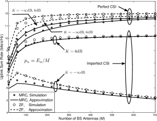
Figure 2: Uplink sum rate per cell versus the number of BS antennas, with $N=10$ users and scaled-down power $p_{u}={E_{u}}/{M}$, where $E_{u}=20$dB.

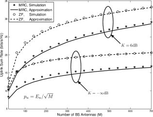
Figure 3: Uplink sum rate per cell versus the number of BS antennas with $N=10$ users and scaled-down power $p_{u}={E_{u}}/{\sqrt{M}}$, where $E_{u}=20$dB.

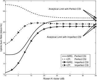
Figure 4: Uplink sum rate per cell versus the Ricean $K$-factor with $N=10$ users, number of BS antennas $M=100$ and transmit power $p_{u}=10$dB.

For our simulations, we consider a cell with a radius of $1000$m and $N$ users distributed randomly and uniformly over the cell, with the exclusion of a central disk of radius $r_{h}=100$m. For convenience, we assume that every user has the same Ricean $K$-factor, denoted by $K$. The large-scale channel fading is modelled using $\beta_{n}={z_{n}}/{\left({r_{n}}/{r_{h}}\right)^{v}}$, where $z_{n}$ is a log-normal random variable with standard deviation $\sigma$, $v$ is the path loss exponent, and $r_{n}$ is the distance between the $n$th user and the BS. We have assumed that $\sigma=8$dB and $v=3.8$. Also, the transmitted data are modulated using orthogonal frequency-division multiplexing (OFDM). The parameters were chosen according to the LTE standard: an OFDM symbol interval of $T_{s}=500/7\approx 71.4\mu$s, a subcarrier spacing of $\Delta_{f}=15k$Hz, a useful symbol duration $T_{u}=1/\Delta_{f}\approx 66.7\mu$s. We choose the channel coherence time to be $T_{c}=1m$s. As a result, the coherence time of the channel becomes $T=\frac{T_{c}}{T_{s}}\frac{T_{u}}{T_{s}-T_{u}}=196$ symbols.

In Fig. 1, the simulated uplink sum rates per cell of MRC and ZF receivers in (31), (47), (71) and (89) are compared with their corresponding analytical approximations in (40), (52), (82) and (98), respectively. Results are presented for two different scenarios – perfect CSI and imperfect CSI. In this example, the number of users $N$ is assumed to be $10$ with the transmit power $p_{u}=10$dB. For each receiver, results are shown for different values of the Ricean $K$-factor, which are $0(-\infty$dB$)$, $3$dB, $6$dB, $10$dB, respectively. Clearly, in all cases, we see a precise agreement between the simulation results and our analytical results. For MRC receivers, as $K$ increases, the sum rate grows obviously for both perfect and imperfect CSI. For ZF receivers, the sum rate has a noticeable growth only with imperfect CSI. We also find that both rates grow without bound, when no power normalization is being performed.

Fig. 2 investigates the power-scaling law when the transmit power of each user is scaled down by ${1}/{M}$. In the simulations, we choose $E_{u}=20$dB and $K$ has two different values, $0(-\infty$dB$)$ and $6$dB. With $p_{u}={E_{u}}/{M}$ and when $M\to\infty$, results show that the analytic approximations are the same as the exact results. In the case of perfect CSI, the sum rates of MRC and ZF receivers approach the same value, independent of the Ricean $K$-factor, as predicted in Section III-A. For imperfect CSI, the sum rates of MRC and ZF receivers always tend to the same value as $M$ becomes large, which depends on $K$. Note that when $K=0$, the sum rates do not have a monotonic behavior. This is because when $M$ is small, $p_{u}$ has not been cut down so much. Therefore, the improvement of the sum rate caused by the increased $M$ is greater than the loss of the sum rate caused by the reduced $p_{u}$. However, as $M$ gets larger, $p_{u}$ is cut down more aggressively. For the case $K=0$ with imperfect CSI, the decay of the sum rate brought by the reduced $p_{u}$ exceeds the growth of the sum rate brought by the increased $M$. Hence, the sum-rate curve will first rise and then drop as increasing $M$. In all other cases, with large $M$, there is a balance between the increase and decrease of the sum rate brought by the increased $M$ and scaling-down $p_{u}$, respectively. Therefore, these curves eventually saturate with an increased $M$. Note that all these observations agree with (81) and (97) and the curves for the case $K=0$ are consistent with the simulation results given by [12, Fig. 2].

In Fig. 3, we consider the same setting as in Fig. 2, but the transmit power for each user is scaled down by a factor of ${1}/{\sqrt{M}}$. For convenience, we only show the results in the case with imperfect CSI. As can be seen, the sum rates of both MRC and ZF receivers converge to deterministic constants when $K=0$ but increase with $M$ when $K\neq 0$, which implies that the transmit power $p_{u}$ can be cut down more, just as predicted in Section III-B. Compared with Fig. 2, we see that ZF performs much better than MRC. This is because ZF performs inherently better than MRC at high signal to noise ratio (SNR) and the transmit power here is only scaled down as $1/\sqrt{M}$, which makes the SNR relatively high. Again, all these observations are consistent with the conclusions in Section III-B. Interestingly, the convergence speed of the curves corresponding to the case $K=0$ is rather slow (approximately $\sqrt{M}$ times slower than that in the case considered in Fig. 2).

To conclude this section, we study how the uplink sum rate varies with the Ricean $K$-factor in Fig. 4. Due to the tightness between the simulated values and the approximations, here we only use the approximations in (40), (52), (82) and (98) for analysis. The parameters were assumed to be $N=10$, $p_{u}=10$dB, and $M=100$. In all cases, as expected, the sum rates approximate the fixed value as $K\to\infty$. The two black dots represent the values obtained by (44) and (61), respectively. The two black stars correspond to the values of the black dots multiplied by a coefficient $\left(T-\tau\right)/T$ for the calculation of the sum rate with imperfect CSI, as defined in (23). It is observed that every dot is indistinguishable from the curve limit, which not only means that our analytical results are accurate, but also that for both MRC and ZF receivers, the sum rates will tend to the same value as $K$ increases for both CSI cases. We also find that the sum rates rise as increases with $K$, except for the case of ZF with perfect CSI. This is because the performance of ZF receivers can be severely limited if the channel matrix is ill-conditioned [35, 36]. For the case of ZF receivers with perfect CSI, we experience no inter-user interference and no estimation-error. When $K$ grows, the channel matrix becomes identical to $\mathbf{\bar{H}}$, whose singular values have a large spread. Then, the condition number of $\mathbf{\bar{H}}$ attains very high values, which implies that is ill-conditioned. However, for the case of ZF with imperfect CSI, the main limiting factor is the estimation error. When $K$ grows large, channel estimation becomes far more robust, since quantities that were random before become deterministic. The same holds true for both cases of MRC receivers, where a higher Ricean $K$-factor reduces the effects of inter-user interference.

V Conclusion

This paper worked out the achievable uplink rate of massive MIMO systems over Ricean fading channels with arbitrary-rank mean. We deduced new, tractable expressions for the uplink rate in the large-antenna limit along with exact approximations. Our analysis incorporated both ZF and MRC receivers and the cases of both perfect and imperfect CSI. These results were used to pursue a detailed analysis of the power-scaling law and of how the uplink rates change with the Ricean $K$-factor. We observed that with no degradation in the rate performance, the transmit power of each user can be at most cut down by a factor of ${1}/{M}$, except for the case of Rayleigh fading channels with imperfect CSI where the transmit power can only be scaled down up to a factor of ${1}/{\sqrt{M}}$. With scaling power and the same CSI quality, it was also shown that the uplink rates of MRC and ZF receivers will tend to the same constant value. Finally, with increasing Ricean $K$-factor and the same receiver, the uplink rates for perfect and imperfect CSI will also converge to the same fixed value.

Appendix A Proof of Lemma 1

We know that

$$\mathbb{E}\left\{\log_{2}\left(1+\frac{X}{Y}\right)\right\}=\mathbb{E}\left\{\log_{2}\left(X+Y\right)\right\}-\mathbb{E}\left\{\log_{2}\left(Y\right)\right\}.$$ (105)

With the Jensen’s inequality, we can get the following bounds:

$$\log_{2}\left(\frac{1}{\mathbb{E}\left\{\frac{1}{X+Y}\right\}}\right)\leq\mathbb{E}\left\{\log_{2}\left(X+Y\right)\right\}\leq\log_{2}\left(\mathbb{E}\left\{X+Y\right\}\right),$$ (106)

and

$$\log_{2}\left(\frac{1}{\mathbb{E}\left\{\frac{1}{Y}\right\}}\right)\leq\mathbb{E}\left\{\log_{2}\left(Y\right)\right\}\leq\log_{2}\left(\mathbb{E}\left\{Y\right\}\right).$$ (107)

Combing (106) and (107), a lower and upper bound on (105) can be obtained as follows

$$\log_{2}\left(\negthickspace\frac{1}{\mathbb{E}\left\{\negthickspace\frac{1}{X+Y}\negthickspace\right\}}\negthickspace\right)-\log_{2}\left(\mathbb{E}\left\{Y\right\}\right)\leq\mathbb{E}\left\{\log_{2}\left(\negmedspace X\negthickspace+\negthickspace Y\negmedspace\right)\right\}-\mathbb{E}\left\{\log_{2}\negmedspace\left(Y\negmedspace\right)\right\}\\ \leq\log_{2}\left(\mathbb{E}\left\{X+Y\right\}\right)-\log_{2}\left(\frac{1}{\mathbb{E}\left\{\frac{1}{Y}\right\}}\right).$$ (108)

Utilizing $\mathbb{E}\left\{\frac{1}{X+Y}\right\}\geq\frac{1}{\mathbb{E}\left\{X+Y\right\}}$ and $\mathbb{E}\left\{\frac{1}{Y}\right\}\geq\frac{1}{\mathbb{E}\left\{Y\right\}}$ and combining them with the left and right hand side of (108), respectively, we get that

$$\log_{2}\left(\negthickspace\frac{1}{\mathbb{E}\left\{\negthickspace\frac{1}{X+Y}\negthickspace\right\}}\negthickspace\right)-\log_{2}\left(\mathbb{E}\left\{Y\right\}\right)\leq\log_{2}\left(\mathbb{E}\negthickspace\left\{\negmedspace X\negthickspace+\negthickspace Y\negmedspace\right\}\right)-\log_{2}\left(\mathbb{E}\left\{Y\right\}\right)\\ \leq\log_{2}\left(\mathbb{E}\left\{X+Y\right\}\right)-\log_{2}\left(\frac{1}{\mathbb{E}\left\{\frac{1}{Y}\right\}}\right).$$ (109)

The above equation can be further written as

$$\log_{2}\left(\frac{1}{\mathbb{E}\left\{\frac{1}{X+Y}\right\}}\right)-\log_{2}\left(\mathbb{E}\left\{Y\right\}\right)\leq\log_{2}\left(1+\frac{\mathbb{E}\left\{X\right\}}{\mathbb{E}\left\{Y\right\}}\right)\\ \leq\log_{2}\left(\mathbb{E}\left\{X+Y\right\}\right)-\log_{2}\left(\frac{1}{\mathbb{E}\left\{\frac{1}{Y}\right\}}\right).$$ (110)

Comparing (108) and (110), we find that $\log_{2}\left(1+\frac{\mathbb{E}\left\{X\right\}}{\mathbb{E}\left\{Y\right\}}\right)$ is a quantity that lies between the upper and lower bound of $\mathbb{E}\left\{\log_{2}\left(1+\frac{X}{Y}\right)\right\}$. Therefore, it can be used as an approximation.

Moreover, we can quantify the offset between these two bounds as

$$d=\log_{2}\left({\mathbb{E}\left\{{X+Y}\right\}\mathbb{E}\left\{{\frac{1}{{X+Y}}}\right\}\mathbb{E}\left\{Y\right\}\mathbb{E}\left\{{\frac{1}{Y}}\right\}}\right).$$ (111)

By applying a Taylor series expansion of $\frac{1}{Y}$ around $\mathbb{E}\left\{Y\right\}$, we get that

$$\mathbb{E}\left\{Y\right\}\mathbb{E}\left\{\frac{1}{Y}\right\}\approx\mathbb{E}\left\{Y\right\}\\ \times\mathbb{E}\left\{\negthickspace{\frac{1}{{\mathbb{E}\negthickspace\left\{Y\right\}}}\negthickspace-\negthickspace\frac{1}{{{{{\mathbb{E}^{2}\negthickspace\left\{Y\right\}}}}}}\left({Y\negthickspace-\negthickspace\mathbb{E}\negthickspace\left\{Y\right\}}\right)\negthickspace+\negthickspace\frac{1}{{{{{\mathbb{E}^{3}\negthickspace\left\{Y\right\}}}}}}{{\left({Y\negthickspace-\negthickspace\mathbb{E}\negthickspace\left\{Y\right\}}\right)}^{2}}}\negthickspace\right\}\\ =1+\frac{1}{\mathbb{E}^{2}\left\{Y\right\}}{\tt Var}\left\{Y\right\}$$ (112)

The substitution of (112) into (111) yields

$$d\approx\log_{2}\left(\left(1+\frac{1}{\mathbb{E}^{2}\left\{X+Y\right\}}{\tt Var}\left\{X+Y\right\}\right)\right.\\ \times\left.\left(1+\frac{1}{\mathbb{E}^{2}\left\{Y\right\}}{\tt Var}\left\{Y\right\}\right)\right).$$ (113)

Since both $X$ and $Y$ are nonnegative, as $t_{1}$ and $t_{2}$ grow large, $\mathbb{E}\left\{X+Y\right\}$ and $\mathbb{E}\left\{Y\right\}$ will increase, and according to the law of large numbers, $X+Y$ and $Y$ will approach their means, that is, their variances will become small. Hence, the offset $d$ decreases with the increase of $t_{1}$ and $t_{2}$, that is, this approximation will be more and more accurate as the number of random variables of $X$ and $Y$ increase.

Appendix B Proof of Lemma 2

According to the law of large numbers, we know that

$$\frac{1}{M}\mathbf{h}_{n}^{H}{\mathbf{h}_{i}}-\frac{1}{M}\sum_{m=1}^{M}\mathbb{E}\left\{{\left[\mathbf{H}\right]_{mn}^{*}{{\left[\mathbf{H}\right]}_{mi}}}\right\}\xrightarrow{a.s.}0.$$ (114)

The entries of $\mathbf{H}$ can be obtained from (4) and (5) described in Section II-A. Hence,

$$\left[\mathbf{H}\right]_{mn} =\sqrt{\frac{K_{n}}{{K_{n}+1}}}{e^{-j\left({m-1}\right)\pi\sin\left({{\theta_{n}}}\right)}}+\sqrt{\frac{1}{{K_{n}+1}}}\left({{s_{mn}}+j{t_{mn}}}\right),$$ (115)

with $s_{mn}$ and $t_{mn}$ representing the independent real and imaginary parts of $\left[{\mathbf{H}_{w}}\right]_{mn}$, respectively, each with zero-mean and variance of ${1}/{2}$. After substituting (115) into (114) and with the definition

$${e^{-j\left({m-1}\right)\pi\sin\left({{\theta_{n}}}\right)}}=\sigma_{mn},\quad{s_{mn}}+j{t_{mn}}=q_{mn},$$ (116)

we have, as $M\to\infty$,

$$\frac{1}{M}\mathbf{h}_{n}^{H}{\mathbf{h}_{i}} -\frac{1}{M\sqrt{\left(K_{n}+1\right)\left(K_{i}+1\right)}}\sum\limits_{m=1}^{M}\mathbb{E}\left\{{\sqrt{K_{n}K_{i}}\sigma_{mn}^{*}{\sigma_{mi}}}\right.$$

$$\left.{+\sqrt{K_{n}}\sigma_{mn}^{*}{q_{mi}}}{+\sqrt{K_{i}}{\sigma_{mi}}q_{mn}^{*}+q_{mn}^{*}{q_{mi}}}\right\}\xrightarrow{a.s.}0.$$ (117)

If $i=n$, it can be easily obtained that $\frac{1}{M}\mathbf{h}_{n}^{H}{\mathbf{h}_{n}}\to 1$. If $i\neq n$, the last three terms of (117) all become zero and the only remaining term is

$$\frac{\sqrt{K_{n}K_{i}}}{M\sqrt{\left(K_{n}+1\right)\left(K_{i}+1\right)}}\sum_{m=1}^{M}{e^{j\left({m-1}\right)\pi\left[{\sin\left({\theta_{n}}\right)-\sin\left({\theta_{i}}\right)}\right]}}\\ \mathop{=}\limits^{(a)}\frac{\sqrt{K_{n}K_{i}}}{M\sqrt{\left(K_{n}+1\right)\left(K_{i}+1\right)}}\phi_{ni}{e^{j\frac{\left({M-1}\right)\pi}{2}\left[{\sin\left({\theta_{n}}\right)-\sin\left({\theta_{i}}\right)}\right]}},$$ (118)

where $\phi_{ni}$ is defined in (29) and $(a)$ is obtained by using [26, Eq. (14)]. Due to the fact that ${{\sin\left({\frac{M\pi}{2}\left[{\sin\left({\theta_{n}}\right)-\sin\left({\theta_{i}}\right)}\right]}\right)}}{e^{j\frac{\left({M-1}\right)\pi}{2}\left[{\sin\left({\theta_{n}}\right)-\sin\left({\theta_{i}}\right)}\right]}}$ is bounded, we get as $M\to\infty$

$$\frac{\sin\left({\frac{M\pi}{2}\left[{\sin\left({\theta_{n}}\right)-\sin\left({\theta_{i}}\right)}\right]}\right)}{M}{e^{j\frac{\left({M-1}\right)\pi}{2}\left[{\sin\left({\theta_{n}}\right)-\sin\left({\theta_{i}}\right)}\right]}}\to 0.$$ (119)

Hence, we arrive at the desired result in (25).

Appendix C Proof of Lemma 3

Using (117) in Appendix B, we first consider the case $i=n$ and we have

$$\mathbf{h}_{n}^{H}\mathbf{h}_{n} =\sum_{m=1}^{M}{\left\{{\frac{K_{n}}{{K_{n}+1}}+\frac{{\sqrt{K_{n}}}}{{K_{n}+1}}\sigma_{mn}^{*}{q_{mn}}{\rm{}}}\right.}$$

$$\left.{+\frac{{\sqrt{K_{n}}}}{{K_{n}+1}}{\sigma_{mn}}q_{mn}^{*}+\frac{1}{{K_{n}+1}}\left({s_{mn}^{2}+t_{mn}^{2}}\right)}\right\}.$$ (120)

Then, it is easily obtained that

$$\mathbb{E}\left\{\mathbf{h}^{H}_{n}\mathbf{h}_{n}\right\}=\sum_{m=1}^{M}\left(\frac{K_{n}}{K_{n}+1}+\frac{1}{K_{n}+1}\right)=M.$$ (121)

To evaluate the norm-square of a vector, we first should extract its real and imaginary parts. Note that $\mathbf{h}_{n}^{H}\mathbf{h}_{n}$ has only real parts. Hence, its norm-square can be obtained by squaring (C) directly as (122) (at the top of the next page).

$$\left\|\mathbf{h}_{n}\right\|^{4} =\left|\mathbf{h}^{H}_{n}\mathbf{h}_{n}\right|^{2}=\frac{{4K_{n}}}{{{{\left({K_{n}+1}\right)}^{2}}}}{\left[{\mathop{\sum}\limits_{m=1}^{M}\left({s_{mn}}\rho^{c}_{mn}-{t_{mn}}\rho^{s}_{mn}\right)}\right]^{2}}+\frac{1}{{{{\left({K_{n}+1}\right)}^{2}}}}{\left[{\mathop{\sum}\limits_{m=1}^{M}\left({s_{mn}^{2}+t_{mn}^{2}}\right)}\right]^{2}}+\frac{{2MK_{n}}}{{{{\left({K_{n}+1}\right)}^{2}}}}\mathop{\sum}\limits_{m=1}^{M}\left({s_{mn}^{2}+t_{mn}^{2}}\right)$$

$$+\frac{{4MK_{n}\sqrt{K_{n}}}}{{{{\left({K_{n}+1}\right)}^{2}}}}\mathop{\sum}\limits_{m=1}^{M}\left({{s_{mn}}\rho^{c}_{mn}}-{t_{mn}}\rho^{s}_{mn}\right)+\frac{{4\sqrt{K_{n}}}}{{{{\left({K_{n}+1}\right)}^{2}}}}\sum\limits_{{m_{1}}=1}^{M}{\sum\limits_{{m_{2}}=1}^{M}{\left({{s_{m_{1}n}}\rho^{c}_{m_{1}n}-{t_{m_{1}n}}\rho^{s}_{m_{1}n}}\right)}}\left({s_{m_{2}n}^{2}+t_{m_{2}n}^{2}}\right)+{\left({\frac{{MK_{n}}}{{K_{n}+1}}}\right)^{2}}.$$ (122)

Applying $\mathbb{E}\left\{\left(s_{mn}\right)^{4}\right\}=\mathbb{E}\left\{\left(t_{mn}\right)^{4}\right\}={3}/{4}$ in (122) and removing all the terms with zero mean, we can get

$$\mathbb{E}\left\{\left\|\mathbf{h}_{n}\right\|^{4}\right\} =\left(\frac{{MK_{n}}}{{K_{n}+1}}\right)^{2}\negthickspace+\negthickspace\frac{2MK_{n}}{\left(K_{n}+1\right)^{2}}\negthickspace+\negthickspace\frac{M^{2}+M}{\left(K_{n}+1\right)^{2}}\negthickspace+\negthickspace\frac{2M^{2}K_{n}}{\left(K_{n}+1\right)^{2}}$$

$$=\frac{2MK_{n}+M}{\left(K_{n}+1\right)^{2}}+M^{2}.$$ (123)

If $i\neq n$, from (117) we know that

$$\mathbf{h}_{n}^{H}\mathbf{h}_{i}=\frac{1}{\sqrt{(K_{n}+1)(K_{i}+1)}}\sum\limits_{m=1}^{M}\left\{{\sqrt{K_{n}K_{i}}\sigma_{mn}^{*}{\sigma_{mi}}}\right.\\ +\left.{\sqrt{K_{n}}\sigma_{mn}^{*}{q_{mi}}}{+\sqrt{K_{i}}{\sigma_{mi}}q_{mn}^{*}+q_{mn}^{*}{q_{mi}}}\right\}.$$ (124)

To obtain the norm-square of (124), both the real and imaginary parts should be extracted. Recalling (118), we can rewrite (124) as

$$\left({\mathbf{h}_{n}^{H}\mathbf{h}_{i}}\right)_{\sf real}\negthickspace =\negthickspace\frac{1}{\sqrt{(K_{n}+1)(K_{i}+1)}}\left\{\negthickspace\sum\limits_{m=1}^{M}{\negthickspace\left[\negthickspace\sqrt{K_{n}}\left({{s_{mi}}\rho^{c}_{mn}\negthickspace-\negthickspace{t_{mi}}\rho^{s}_{mn}}\right)\right.}\right.$$

$$+\left.{\left.\sqrt{K_{i}}\left({s_{mn}}\rho^{c}_{mi}-{t_{mn}}\rho^{s}_{mi}\right)+\left({{s_{mn}}{s_{mi}}+{t_{mn}}{t_{mi}}}\right)\right]}\right.$$

$$+\left.\sqrt{K_{n}K_{i}}\phi_{ni}\cos\left({\frac{{M-1}}{2}\pi\left[{\sin\left({{\theta_{n}}}\right)-\sin\left({{\theta_{i}}}\right)}\right]}\right)\right\},$$ (125)

$$\left({\mathbf{h}_{n}^{H}\mathbf{h}_{i}}\right)_{\sf imag}\negthickspace =\negthickspace\frac{1}{\sqrt{(K_{n}+1)(K_{i}+1)}}\left\{\negthickspace\sum\limits_{m=1}^{M}\negthickspace\left[\sqrt{K_{n}}\left({{t_{mi}}\rho^{c}_{mn}\negthickspace+\negthickspace{s_{mi}}\rho^{s}_{mn}}\right)\right.\right.$$

$$-\left.\sqrt{K_{i}}\left({s_{mn}}\rho^{s}_{mi}+{t_{mn}}\rho^{c}_{mi}\right)+{\left({{s_{mn}}{t_{mi}}-{t_{mn}}{s_{mi}}}\right)}\right]$$

$$+\left.\sqrt{K_{n}K_{i}}\phi_{ni}\sin\left({\frac{{M-1}}{2}\pi\left[{\sin\left({{\theta_{n}}}\right)-\sin\left({{\theta_{i}}}\right)}\right]}\right)\right\}.$$ (126)

Then, with

$$\mathbb{E}\left\{\left|\mathbf{h}_{n}^{H}\mathbf{h}_{i}\right|^{2}\right\}=\mathbb{E}\left\{\left({\mathbf{h}_{n}^{H}\mathbf{h}_{i}}\right)_{\sf real}^{2}+\left({\mathbf{h}_{n}^{H}\mathbf{h}_{i}}\right)_{\sf imag}^{2}\right\},$$ (127)

substituting (125) and (126) into (127) and removing the terms with zero expectation, we get the final result as

$$\mathbb{E}\left\{\left|\mathbf{h}_{n}^{H}\mathbf{h}_{i}\right|^{2}\right\}=\frac{{{K_{n}K_{i}}{\phi^{2}_{ni}}+M\left(K_{n}+K_{i}\right)+M}}{{{{\left({K_{n}+1}\right)\left(K_{i}+1\right)}}}}.$$ (128)

As we have obtained all expectations used in Lemma 3, we now conclude the proof.

Appendix D Proof of Lemma 4

Following the similar procedure as in the proof of Lemma 2, we start by giving the entries of the channel matrix. The imperfect CSI model has been described in (12) of Section II-B2, which yields

$${\left[\mathbf{\hat{G}}\right]_{mn}}=\sqrt{\frac{K_{n}}{{K_{n}+1}}}{\left[\mathbf{\bar{G}}\right]_{mn}}+\sqrt{\frac{1}{{K_{n}+1}}}{\left[{{{\mathbf{\hat{G}}}_{w}}}\right]_{mn}}.$$ (129)

The first term which does not need to be estimated is the same as in the case with perfect CSI. For $\mathbf{\hat{G}}_{w}$, we use the MMSE estimation to get it and the details of the method have been introduced in Section II-B2. Therefore, we have

$${\left[\mathbf{\hat{G}}\right]_{mn}} =\sqrt{\frac{K_{n}}{{K_{n}+1}}}\sqrt{{\beta_{n}}}{\sigma_{mn}}$$

$$+\sqrt{\frac{1}{{K_{n}+1}}}{\eta_{n}}\left[{\sqrt{{\beta_{n}}}{q_{mn}}+\frac{1}{{\sqrt{{p_{p}}}}}\left({s{w_{mn}}+jt{w_{mn}}}\right)}\right]$$ (130)

where $\sigma_{mn}$, $s_{mn}$ and $t_{mn}$ have all been defined in (116) of Appendix C, $sw_{mn}$ and $tw_{mn}$ represent the independent real and imaginary part of $\left[\mathbf{W}\right]_{mn}$ with zero-mean and variance ${1}/{2}$, and $\eta_{n}$ is defined in (68). By the law of large numbers, it can be got that

$$\frac{1}{M}\mathbf{\hat{g}}_{n}^{H}{{\mathbf{\hat{g}}}_{n}}-\frac{1}{M}\sum\limits_{m=1}^{M}\mathbb{E}{\left\{{\left[\mathbf{\hat{G}}\right]_{mn}^{*}{{\left[\mathbf{\hat{G}}\right]}_{mn}}}\right\}}\xrightarrow{a.s.}0.$$ (131)

With (131) and the definition

$$sw_{mn}+jtw_{mn}=qw_{mn},$$ (132)

we can obtain (133) (at the top of the next page), as $M\to\infty$,

$$\frac{1}{M}\mathbf{\hat{g}}_{n}^{H}{{\mathbf{\hat{g}}}_{n}} -\frac{1}{M}\sum\limits_{m=1}^{M}\mathbb{E}\left\{\frac{K_{n}}{{K_{n}+1}}{\beta_{n}}+\frac{{\sqrt{K_{n}}}}{{K_{n}+1}}\sqrt{{\beta_{n}}}{\eta_{n}}\sigma_{mn}^{*}\left({\sqrt{{\beta_{n}}}{q_{mn}}+\frac{1}{{\sqrt{{p_{p}}}}}q{w_{mn}}}\right)+\frac{1}{{K_{n}+1}}\frac{\sqrt{\eta_{n}^{2}\beta_{n}}}{\sqrt{p_{p}}}\left({q_{mn}^{*}q{w_{mn}}+{q_{mn}}qw_{mn}^{*}}\right)\right.$$

$$+\frac{{\sqrt{K_{n}}}}{{K_{n}+1}}\sqrt{{\beta_{n}}}{\eta_{n}}{\sigma_{mn}}\left({\sqrt{{\beta_{n}}}q_{mn}^{*}+\frac{1}{{\sqrt{{p_{p}}}}}qw_{mn}^{*}}\right)\left.+\frac{1}{{K_{n}+1}}\eta_{n}^{2}\left[{{\beta_{n}}\left({s_{mn}^{2}+t_{mn}^{2}}\right)}+\frac{1}{p_{p}}\left(sw_{mn}^{2}+tw_{mn}^{2}\right)\right]\right\}\xrightarrow{a.s.}0.$$ (133)

Evaluating the expectation of all terms in (133) and removing the terms with zero expectation, (133) can be simplified as

$$\frac{1}{M}\mathbf{\hat{g}}_{n}^{H}{{\mathbf{\hat{g}}}_{n}}-\\ \frac{1}{M}\sum_{m=1}^{M}\left[\frac{K_{n}}{K_{n}+1}\beta_{n}+\frac{1}{K_{n}+1}\eta_{n}^{2}\left(\beta_{n}+\frac{1}{p_{p}}\right)\right]\xrightarrow{a.s.}0,$$ (134)

which yields that

$$\frac{1}{M}\mathbf{\hat{g}}_{n}^{H}{{\mathbf{\hat{g}}}_{n}}\xrightarrow{a.s.}\frac{\beta_{n}}{K_{n}+1}\left(K_{n}+\eta_{n}\right).$$ (135)

Now consider $\mathbf{\hat{g}}_{n}^{H}\mathbf{\hat{g}}_{i}$. Following the same operations as in (133), with

$$\frac{1}{M}\mathbf{\hat{g}}_{n}^{H}{{\mathbf{\hat{g}}}_{i}}-\frac{1}{M}\sum\limits_{m=1}^{M}\mathbb{E}{\left\{{\left[\mathbf{\hat{G}}\right]_{mn}^{*}{{\left[\mathbf{\hat{G}}\right]}_{mi}}}\right\}}\xrightarrow{a.s.}0$$ (136)

we find (137) (at the top of the next page).

$$\frac{1}{M}\mathbf{\hat{g}}_{n}^{H}{{\mathbf{\hat{g}}}_{i}} -\frac{1}{M\sqrt{(K_{n}+1)(K_{i}+1)}}\sum\limits_{m=1}^{M}\mathbb{E}\left\{\sqrt{K_{n}K_{i}}\sqrt{{\beta_{n}}{\beta_{i}}}\sigma_{mn}^{*}{\sigma_{mn}}+\sqrt{K_{n}}\sqrt{{\beta_{n}}}{\eta_{i}}\sigma_{mn}^{*}\left({\sqrt{{\beta_{i}}}{q_{mi}}+\frac{1}{{\sqrt{{p_{p}}}}}q{w_{mi}}}\right)\right.$$

$$\left.+\sqrt{K_{i}}\sqrt{{\beta_{i}}}{\eta_{n}}{\sigma_{mi}}\left({\sqrt{{\beta_{n}}}q_{mn}^{*}+\frac{1}{{\sqrt{{p_{p}}}}}qw_{mn}^{*}}\right)+{\eta_{n}}{\eta_{i}}\left({q_{mn}^{*}{q_{mi}}+qw_{mn}^{*}q{w_{mi}}+q_{mn}^{*}q{w_{mi}}+{q_{mi}}qw_{mn}^{*}}\right)\right\}\xrightarrow{a.s.}0.$$ (137)

Since the entries of $\mathbf{H}$ and $\mathbf{W}$ are all i.i.d. zero-mean with unit-variance, many terms in (137) have zero expectation. The only remaining term is the element of the channel mean matrix. Hence, (137) can be written as

$$\frac{1}{M}\mathbf{\hat{g}}_{n}^{H}{{\mathbf{\hat{g}}}_{i}}-\\ \frac{1}{M}\sum\limits_{m=1}^{M}\frac{\sqrt{K_{n}K_{i}}}{{\sqrt{(K_{n}+1)(K_{i}+1)}}}\sqrt{{\beta_{n}}{\beta_{i}}}\sigma_{mn}^{*}{\sigma_{mi}}\xrightarrow{a.s.}0,$$ (138)

which can be simplified as

$$\frac{1}{M}\mathbf{\hat{g}}_{n}^{H}{{\mathbf{\hat{g}}}_{i}}-\\ \frac{\sqrt{{\beta_{n}}{\beta_{i}}}\sqrt{K_{n}K_{i}}\phi_{ni}}{M\sqrt{(K_{n}+1)(K_{i}+1)}}e^{\frac{M-1}{2}\pi\left[\sin\left(\theta_{n}\right)-\sin\left(\theta_{i}\right)\right]}\xrightarrow{a.s.}0.$$ (139)

According to (119), we know that, as $M\to\infty$

$$\frac{\phi_{ni}}{M}e^{\frac{M-1}{2}\pi\left[\sin\left(\theta_{n}\right)-\sin\left(\theta_{i}\right)\right]}\to 0.$$ (140)

As a consequence, (139) can be further simplified as

$$\frac{1}{M}\mathbf{\hat{g}}_{n}^{H}\mathbf{\hat{g}}_{i}\xrightarrow{a.s.}0.$$ (141)

Appendix E Proof of Lemma 5

The expectation of $\mathbf{\hat{g}}_{n}^{H}\mathbf{\hat{g}}_{n}$ can be easily obtained by (134) in Appendix D. Hence, we have

$$\mathbb{E}\left\{\mathbf{\hat{g}}_{n}^{H}\mathbf{\hat{g}}_{n}\right\}=\frac{M\beta_{n}}{K_{n}+1}\left(K_{n}+\eta_{n}\right).$$ (142)

Following the same procedure as in the proof of Lemma 3, we can obtain the remaining three norm-square expectations. First consider the case $i=n$. According to (133), we have (143) (at the top of the next page).

$$\mathbb{E}\left\{\left|\mathbf{\hat{g}}_{n}^{H}\mathbf{\hat{g}}_{n}\right|^{2}\right\} =\mathbb{E}\left\{\sum\limits_{m=1}^{M}\frac{K_{n}}{{K_{n}+1}}{\beta_{n}}+\frac{{\sqrt{K_{n}}}}{{K_{n}+1}}\sqrt{{\beta_{n}}}{\eta_{n}}\sigma_{mn}^{*}\left[{\sqrt{{\beta_{n}}}{q_{mn}}+\frac{1}{{\sqrt{{p_{p}}}}}q{w_{mn}}}\right]+\frac{1}{{K_{n}+1}}\eta_{n}^{2}\left({q_{mn}^{*}q{w_{mn}}+{q_{mn}}qw_{mn}^{*}}\right)\right.$$

$$\left.+\frac{{\sqrt{K_{n}}}}{{K_{n}+1}}\sqrt{{\beta_{n}}}{\eta_{n}}{\sigma_{mn}}\left[{\sqrt{{\beta_{n}}}q_{mn}^{*}+\frac{1}{{\sqrt{{p_{p}}}}}qw_{mn}^{*}}\right]+\frac{1}{{K_{n}+1}}\eta_{n}^{2}\left[{{\beta_{n}}\left({s_{mn}^{2}+t_{mn}^{2}}\right)}+\frac{1}{p_{p}}\left(sw_{mn}^{2}+tw_{mn}^{2}\right)\right]\right\}^{2}.$$ (143)

After expanding the above equation and removing all the terms with zero expectation, the remaining terms are written as (144) (at the top of the next page).

$$\mathbb{E}\left\{\left|\mathbf{\hat{g}}_{n}^{H}\mathbf{\hat{g}}_{n}\right|^{2}\right\} ={\left({\frac{{MK_{n}}}{{K_{n}+1}}}\right)^{2}}\beta_{n}^{2}+\frac{{2MK_{n}}}{{{{\left({K_{n}+1}\right)}^{2}}}}{\beta_{n}}\eta_{n}^{2}\left({{\beta_{n}}+\frac{1}{{{p_{p}}}}}\right)+\frac{{2M{\beta_{n}}}}{{{{\left({K_{n}+1}\right)}^{2}}}}\eta_{n}^{4}+\left({{M^{2}}+M}\right)\left({\beta_{n}^{2}+\frac{1}{{p_{p}^{2}}}}\right)\frac{{\eta_{n}^{4}}}{{{{\left({K_{n}+1}\right)}^{2}}}}$$

$$+\frac{{2{M^{2}}K_{n}\eta_{n}^{2}}}{{{{\left({K_{n}+1}\right)}^{2}}}}\left({\beta_{n}^{2}+\frac{{{\beta_{n}}}}{{{p_{p}}}}}\right)+\frac{{2{M^{2}}\eta_{n}^{4}}}{{{{\left({K_{n}+1}\right)}^{2}}}}\frac{{{\beta_{n}}}}{{{p_{p}}}}=\frac{{\beta_{n}^{2}}}{{{{\left({K_{n}+1}\right)}^{2}}}}\left[{{M^{2}}{K_{n}^{2}}+\left({2MK_{n}+2M^{2}{K_{n}}}\right){\eta_{n}}+\left({{M^{2}}+M}\right)\eta_{n}^{2}}\right].$$ (144)

For the case $i\neq n$, we use the same method as in the proof of Lemma 3. With (137), it is noted that the inner product $\mathbf{\hat{g}}_{n}^{H}\mathbf{\hat{g}}_{i}$ has non-zero real and imaginary parts. The result then follows trivially by some algebraic manipulations.

Qi Zhang received the B.S. degree in Electrical & Information Engineering from Nanjing University of Posts & Telecommunications, Nanjing, China, in 2010. She is currently working toward the Ph.D. degree in Communication & Information System at the Nanjing University of Posts & Telecommunications, China. Her research interests include massive MIMO systems and space-time wireless communications.

Shi Jin (S’06-M’07) received the B.S. degree in communications engineering from Guilin University of Electronic Technology, Guilin, China, in 1996, the M.S. degree from Nanjing University of Posts and Telecommunications, Nanjing, China, in 2003, and the Ph.D. degree in communications and information systems from the Southeast University, Nanjing, in 2007. From June 2007 to October 2009, he was a Research Fellow with the Adastral Park Research Campus, University College London, London, U.K. He is currently with the faculty of the National Mobile Communications Research Laboratory, Southeast University. His research interests include space time wireless communications, random matrix theory, and information theory. He serves as an Associate Editor for the IEEE Transactions on Wireless Communications, and IEEE Communications Letters, and IET Communications. Dr. Jin and his co-authors have been awarded the 2011 IEEE Communications Society Stephen O. Rice Prize Paper Award in the field of communication theory and a 2010 Young Author Best Paper Award by the IEEE Signal Processing Society.

Kai-Kit Wong (S’99-M’01-SM’08) received the BEng, the MPhil, and the PhD degrees, all in Electrical and Electronic Engineering, from the Hong Kong University of Science & Technology, Hong Kong, in 1996, 1998, and 2001, respectively. Since August 2006, he has been with University College London, first at Adastral Park Campus and at present the Department of Electronic & Electrical Engineering, where he is a Reader in Wireless Communications. Dr Wong is a Senior Member of IEEE and Fellow of the IET. He is on the editorial board of IEEE Wireless Communications Letters, IEEE Communications Letters, IEEE ComSoc/KICS Journal of Communications and Networks, and IET Communications. He also previously served as Editor for IEEE Transactions on Wireless Communications from 2005-2011 and IEEE Signal Processing Letters from 2009-2012.

Hongbo Zhu received the bachelor degree in Telecommunications Engineering from the Nanjing University of Posts & Telecommunications, Nanjing, China and Ph.D. degree in Information & Communications Engineering from Beijing University of Posts & Telecommunications, Beijing, China, in 1982 and 1996, respectively. He is presently working as a Professor and Vice-president in Nanjing University of Posts & Telecommunications, Nanjing, China. He is also the head of the Coordination Innovative Center of IoT Technology and Application (Jiangsu), which is the first governmental authorized Coordination Innovative Center of IoT in China. He also serves as referee or expert in multiple national organizations and committees. He has published more than 200 papers on information and communication area, such as IEEE Trans. Presently, he is leading a big group and multiple funds on IoT and wireless communications with current focus on architecture and enabling technologies for Internet of Things.

Michail Matthaiou (S’05–M’08–SM’13) was born in Thessaloniki, Greece in 1981. He obtained the Diploma degree (5 years) in Electrical and Computer Engineering from the Aristotle University of Thessaloniki, Greece in 2004. He then received the M.Sc. (with distinction) in Communication Systems and Signal Processing from the University of Bristol, U.K. and Ph.D. degrees from the University of Edinburgh, U.K. in 2005 and 2008, respectively. From September 2008 through May 2010, he was with the Institute for Circuit Theory and Signal Processing, Munich University of Technology (TUM), Germany working as a Postdoctoral Research Associate. He is currently a Senior Lecturer at Queen’s University Belfast, U.K. and also holds an adjunct Assistant Professor position at Chalmers University of Technology, Sweden. His research interests span signal processing for wireless communications, massive MIMO, hardware-constrained communications, and performance analysis of fading channels. Dr. Matthaiou is the recipient of the 2011 IEEE ComSoc Young Researcher Award for the Europe, Middle East and Africa Region and a co-recipient of the 2006 IEEE Communications Chapter Project Prize for the best M.Sc. dissertation in the area of communications. He was an Exemplary Reviewer for IEEE Communications Letters for 2010. He has been a member of Technical Program Committees for several IEEE conferences such as ICC, GLOBECOM, VTC etc. He currently serves as an Associate Editor for the IEEE Transactions on Communications, IEEE Communications Letters and was the Lead Guest Editor of the special issue on “Large-scale multiple antenna wireless systems” of the IEEE Journal on Selected Areas in Communications. He is an associate member of the IEEE Signal Processing Society SPCOM and SAM technical committees.

References

• [1] A. Paulraj, R. Nabar, and D. Gore, Introduction to Space-time Wireless Communications.   Cambridge University Press, 2003.
• [2] D. N. C. Tse and P. Viswanath, Fundamentals of Wireless Communication.   Cambridge University Press, 2005.
• [3] D. Gesbert, M. Kountouris, R. W. Heath Jr., C.-B. Chae, and T. Salzer, “Shifting the MIMO paradigm,” IEEE Signal Process. Mag., vol. 24, no. 5, pp. 36–46, Sept. 2007.
• [4] P. Viswanath and D. N. C. Tse, “Sum capacity of the vector Gaussian broadcast channel and uplink-downlink duality,” IEEE Trans. Inf. Theory, vol. 49, no. 8, pp. 1912–1921, Aug. 2003.
• [5] G. Caire, N. Jindal, M. Kobayashi, and N. Ravindran, “Multiuser MIMO achievable rates with downlink training and channel state feedback,” IEEE Trans. Inf. Theory, vol. 56, no. 6, pp. 2845–2866, June 2010.
• [6] J. Jose, A. Ashikhmin, T. L. Marzetta, and S. Vishwanath, “Pilot contamination and precoding in multi-cell TDD systems,” IEEE Trans. Wireless Commun., vol. 10, no. 8, pp. 2640–2651, Aug. 2011.
• [7] F. Rusek, D. Persson, B. K. Lau, E. G. Larsson, T. L. Marzetta, O. Edfors, and F. Tufvesson, “Scaling up MIMO: Opportunities and challenges with very large arrays,” IEEE Signal Process. Mag., vol. 30, no. 1, pp. 40–60, Jan. 2013.
• [8] I. E. Telatar, “Capacity of multi-antenna Gaussian channels,” Europ. Trans. Commun., pp. 585–595, Nov.-Dec. 1999.
• [9] T. L. Marzetta, “How much training is required for multiuser MIMO?” in Proc. Asilomar Conf. Signals, Systems, Comput., Oct. 2006, pp. 359–363.
• [10] ——, “Noncooperative cellular wireless with unlimited numbers of base station antennas,” IEEE Trans. Wireless Commun., vol. 9, no. 11, pp. 3590–3600, Nov. 2010.
• [11] J. Hoydis, S. ten Brink, and M. Debbah, “Massive MIMO in the UL/DL of cellular networks: How many antennas do we need?” IEEE J. Sel. Areas Commun., vol. 31, no. 2, pp. 160–171, Feb. 2013.
• [12] H. Q. Ngo, E. G. Larsson, and T. L. Marzetta, “Energy and spectral efficiency of very large multiuser MIMO systems,” IEEE Trans. Commun., vol. 61, no. 4, pp. 1436–1449, Apr. 2013.
• [13] A. Pitarokoilis, S. K. Mohammed, and E. G. Larsson, “On the optimality of single-carrier transmission in large-scale antenna systems,” IEEE Wireless Commun. Lett., vol. 1, no. 4, pp. 276–279, Aug. 2012.
• [14] S. Wagner, R. Couillet, D. T. M. Slock, and M. Debbah, “Large system analysis of zero-forcing precoding in MISO broadcast channels with limited feedback,” in Proc. IEEE Int. Work. Signal Process. Adv. Wireless Commun. (SPAWC), June 2010.
• [15] A. M. Sayeed and N. Behdad, “Continuous aperture phased MIMO: A new architecture for optimum line-of-sight links,” in Proc. IEEE Int. Symp. Ant. Propag. (APS), July 2011, pp. 293–296.
• [16] J. Brady, N. Behdad, and A. M. Sayeed, “Beamspace MIMO for millimeter-wave communications: System architecture, modeling, analysis, and measurements,” IEEE Trans. Antennas Propagat., vol. 61, no. 7, pp. 3814–3827, July 2013.
• [17] A. M. Sayeed and J. Brady, “Beamspace MIMO for high-dimensional multiuser communication at millimeter-wave frequencies,” in Proc. IEEE Global Telecommun. Conf. (GLOBECOM), Dec. 2013.
• [18] A. Lozano, A. M. Tulino, and S. Verdú, “Multiple-antenna capacity in the low-power regime,” IEEE Trans. Inf. Theory, vol. 49, no. 10, pp. 2527–2544, Oct. 2003.
• [19] S. Jin, X. Q. Gao, and X. H. You, “On the ergodic capacity of rank-1 Ricean fading MIMO channels,” IEEE Trans. Inf. Theory, vol. 53, no. 2, pp. 502–517, Feb. 2007.
• [20] J. Zhang, C. K. Wen, S. Jin, X. Gao, and K.-K. Wong, “On capacity of large-scale MIMO multiple access channels with distributed sets of correlated antennas,” IEEE J. Sel. Areas Commun., vol. 31, no. 2, pp. 133–148, Feb. 2013.
• [21] C. K. Wen, S. Jin, and K.-K. Wong, “On the sum-rate of multiuser MIMO uplink channels with jointly-correlated Rician fading,” IEEE Trans. Commun., vol. 59, no. 10, pp. 2883–2895, Oct. 2011.
• [22] C. K. Wen, K.-K. Wong, and J. C. Chen, “Asymptotic mutual information for Rician MIMO-MA channels with arbitrary inputs: A replica analysis,” IEEE Trans. Commun., vol. 58, no. 10, pp. 2782–2788, Oct. 2010.
• [23] J. G. Proakis, Digital Communications, 4th ed.   McGraw-Hill, 2001.
• [24] G. Alfano, A. Lozano, A. M. Tulino, and S. Verdú, “Mutual information and eigenvalue distribution of MIMO Ricean channels,” in Proc. IEEE Int. Symp. Inf. Theory Appl. (ISITA), Oct. 2004, pp. 10–13.
• [25] M. Matthaiou, C. Zhong, and T. Ratnarajah, “Novel generic bounds on the sum rate of MIMO ZF receivers,” IEEE Trans. Signal Process., vol. 59, no. 9, pp. 4341–4353, Sept. 2011.
• [26] N. Ravindran, N. Jindal, and H. C. Huang, “Beamforming with finite rate feedback for LOS MIMO downlink channels,” in Proc. IEEE Global Commun. Conf. (GLOBECOM), Nov. 2007, pp. 4200–4204.
• [27] E. Torkildson, U. Madhow, and M. Rodwell, “Indoor millimeter wave MIMO: Feasibility and performance,” IEEE Trans. Wireless Commun., vol. 10, no. 12, pp. 4150–4160, Dec. 2011.
• [28] S. M. Kay, Fundamentals of statistical signal processing: Estimation Theory (volume 1).   Prentice Hall, 1993.
• [29] C. Wang, E. Au, R. Murch, W. Mow, R. Cheng, and V. Lau, “On the performance of the MIMO zero-forcing receiver in the presence of channel estimation error,” IEEE Trans. Wireless Commun., vol. 6, no. 3, pp. 805–810, Mar. 2007.
• [30] A. M. Tulino and S. Verdú, “Random matrix theory and wireless communications,” Foundations and Trends in Communicaations and Information Theory, vol. 1, no. 1, pp. 1–182, June 2004.
• [31] H. Steyn and J. Roux, “Approximations for the non-central Wishart distribution,” South African Statist J., vol. 6, pp. 165–173, 1972.
• [32] M. Matthaiou, M. R. McKay, P. J. Smith, and J. A. Nossek, “On the condition number distribution of complex Wishart matrices,” IEEE Trans. Commun., vol. 58, no. 6, pp. 1705–1717, June 2010.
• [33] C. Siriteanu, Y. Miyanaga, S. D. Blostein, S. Kuriki, and X. Shi, “MIMO zero-forcing detection analysis for correlated and estimated Rician fading,” IEEE Trans. Veh. Technol., vol. 61, no. 7, pp. 3087–3099, Sept. 2012.
• [34] D. Gore, R. W. Heath Jr., and A. Paulraj, “Transmit selection in spatial multiplexing systems,” IEEE Commun. Lett., vol. 6, no. 11, pp. 491–493, Nov. 2002.
• [35] E. G. Larsson, “MIMO detection methods: How they work,” IEEE Signal Process. Mag., vol. 26, no. 3, pp. 91–95, May 2009.
• [36] H. Artes, D. Seethaler, and F. Hlawatsch, “Efficient detection algorithms for MIMO channels: A geometrical approach to approximate ML detection,” IEEE Trans. Signal Process., vol. 51, no. 11, pp. 2808–2820, Nov. 2003.