Modulus stabilization in higher curvature dilaton gravity

Abstract

We propose a framework of modulus stabilization in two brane warped geometry scenario in presence of higher curvature gravity and dilaton in bulk space-time. In the prescribed setup we study various features of the stabilized potential for the modulus field, generated by a bulk scalar degrees of freedom with quartic interactions localized on the two 3-branes placed at the orbifold fixed points. We determine the parameter space for the gravidilaton and Gauss-Bonnet couplings required to stabilize the modulus in such higher curvature dilaton gravity setup.

1 Introduction

The Gauss-Bonnet (GB) dilaton gravity is known to be an active area of research in theoretical physics through decades, which was proposed to include the perturbative effects within effective theory based on the well known Einstein’s gravity at the two-loop level [1, 2, 3, 4, 5, 6]. For such theories the two-loop effective coupling signifies the strength of the self-interaction between the spin 2 graviton degrees of freedom below the Ultra-Violet (UV) cut-off of the quantum theory of gravity. Usually such corrections originate naturally in string theory where power expansion in terms of inverse of Regge slope (or string tension) yields the higher curvature corrections to pure Einstein’s gravity. Supergravity, as the low energy limit [7, 8, 9, 10, 11, 12, 13, 14, 15, 16, 17, 18] of heterotic string theory [19, 20, 21, 22, 23, 24, 25, 26, 27], yields the Gauss-Bonnet (GB) term along with dilaton coupling at the leading order correction. Consequently it became an active area of interest as a modified theory of gravity. In the context of black hole it has been shown that GB correction suppresses graviton emission which makes the black hole more stable.The correction to black hole entropy due to GB term has also been explored.Moreover in search of extra dimensions, GB dilaton term in a warped braneworld model has been studied in the context of first kaluza-klein graviton decay channel investigated by ATLAS group in LHC experiments. Thus the Gauss-Bonnet dilaton gravity as a modified gravity theory has been studied extensively in different contexts as a first step to include the higher curvature effects over Einstein’ gravity.

Stability of the modulus in such models is an important issue from phenomenological point of view. Goldberger and Wise (GW) [28, 29, 30] first explicitly showed that the dynamics of a five dimensional bulk scalar field in Randall Sundrum (RS) two brane setup can stabilize the size of the fifth (extra) dimension to a permissible value to solve the gauge hierarchy problem. In this paper we examine such scenario in the context of higher curvature gravity, where the usual Einstein’s gravity is modified by the perturbative GB coupling and dilaton coupling. In this theoretical prescription the stabilized effective potential for the bulk modulus is generated by the presence of a bulk scalar field with quartic self interactions localized in two 3-branes. This results in a modulus potential which after minimization yields a compactification scale in terms of the VEV’s of the scalar fields at the two branes. This concomitantly solves the gauge hierarchy problem without introducing any fine tuning of the model parameters in the prescribed theoretical setup. Here we extend this study to include higher curvature-dilaton term in the bulk space-time where we neglect the effects of back reaction of the bulk scalar on the geometry as was done in case of the original GW mechanism.Some critical studies have been made in this context [31, 32, 33, 34, 35]. Broad aspects of the moduli stabilization mechanism in higher dimensions [36, 37, 38, 39], specifically in the context of cosmological studies [40, 41, 42, 43] from braneworlds i.e. inflation, dark energy and with non minimal scalar fields coupled to the gravity sector have been reported in [44, 45, 46, 47, 48, 49, 50, 51, 52].

The plan of this paper is as follows: In section 2 we study the framework of the modulus stabilization mechanism in the context of GB dilaton gravity. First we propose the background model in higher curvature gravity from which we compute the the expression of the warp factor. Further using this warped solution we determine the analytical expression for the stabilized potential for the bulk modulus field. To check the consistency of our present analysis we then study our setup in three distinct limiting situations namely in RS limit and limit when either of GB coupling or dilaton coupling is present.

2 Modulus Stabilization Mechanism in Gauss-Bonnet dilaton gravity

Here we generalize the analysis of modulus stabilization mechanism in warped geometry in presence of Gauss-Bonnet coupling and gravidilaton coupling in a 5D bulk. The background warped geometry model is proposed by making use of the following sets of assumptions:

• The leading order Einstein’s gravity sector is modified by the Gauss-Bonnet [53, 54, 55, 56, 57, 58, 60, 61, 62, 63] and dilaton coupling [56, 57, 58, 59] which originates from heterotic string theory.

• The background warped metric has a RS like structure [64, 65] on a slice of ${\bf AdS_{5}}$ geometry. For example, from 10-dimensional string model compactified on ${\bf AdS_{5}\times S^{5}}$, one typically obtains moduli from ${\bf S^{5}}$ as scalar degrees of freedom. Such moduli can be stabilized by fluxes. In our model, which is similar to a 5-dimensional Randall-Sundrum (RS) model, it is assumed that these degrees of freedom are frozen to their VEV and are non-dynamical at the energy scale under consideration [66]. We therefore focus into the slice of ${\bf AdS_{5}}$ as is done for the 5-dimensional RS model.

• The dilaton degrees of freedom is assumed to be confined within the bulk.

• We allow the interaction between dilaton and the 5D bulk cosmological constant via dilaton coupling.

• The Higgs field is localized at the visible (TeV) brane and the hierarchy problem is resolved via Planck to TeV scale warping.

• Additionally while determining the values of the model parameters we require that the bulk curvature to be less than the five dimensional Planck scale $M_{5}$ so that the classical solution of the 5-dimensional gravitational equations can be trusted [67, 68].

2.1 The background setup

We start our discussion with the following 5D action of the two brane warped geometry model [58]:

$$\begin{array}[]{llll}\displaystyle S=\int d^{5}x\left[\sqrt{-g_{(5)}}\left\{\frac{M^{3}_{(5)}}{2}R_{(5)}+\frac{\alpha_{(5)}M_{(5)}}{2}\left[R^{ABCD(5)}R^{(5)}_{ABCD}-4R^{AB(5)}R^{(5)}_{AB}+R^{2}_{(5)}\right]\right.\right.\\ \left.\left.\displaystyle~{}~{}~{}~{}~{}~{}~{}~{}~{}~{}~{}~{}~{}~{}~{}~{}~{}~{}~{}~{}~{}~{}~{}~{}~{}~{}~{}+\frac{g^{AB}}{2}\partial_{A}\Phi\partial_{B}\Phi-\frac{m^{2}_{\Phi}}{2}\Phi^{2}+\frac{g^{AB}}{2}\partial_{A}\chi(y)\partial_{B}\chi(y)-2\Lambda_{5}e^{\chi(y)}\right\}\right.\\ \left.\displaystyle~{}~{}~{}~{}~{}~{}~{}~{}~{}~{}~{}~{}~{}~{}~{}~{}~{}~{}~{}~{}~{}~{}~{}~{}~{}~{}~{}~{}~{}~{}~{}~{}~{}~{}~{}~{}~{}~{}~{}~{}~{}~{}~{}~{}~{}~{}~{}~{}-\displaystyle\sum^{2}_{i=1}\sqrt{-g^{(i)}_{(5)}}\left[\lambda_{i}\left(\Phi^{2}-{\cal V}^{2}_{i}\right)^{2}+T_{i}\right]\delta(y-y_{i})\right]\end{array}$$ (2.1)

with $A,B,C,D=0,1,2,3,4$. Here $i$ signifies the brane index, $i=1(\text{hidden})$, $2(\text{visible})$. ${\cal V}_{i}$ and $\lambda_{i}$ signifies the VEV and self coupling of the bulk scalar fields on the ith brane where $T_{i}$ is the brane tension and $\Phi$ represent the bulk scalar degrees of freedom. Additionally $\alpha_{5}$ and $\chi(y)$ represent the GB coupling and dilaton field. The background metric describing slice of the ${\bf AdS_{5}}$ is given by,

$$\begin{array}[]{llllll}\displaystyle ds^{2}_{5}=g_{AB}dx^{A}dx^{B}=e^{-2A(y)}\eta_{\alpha\beta}dx^{\alpha}dx^{\beta}+r^{2}_{c}dy^{2}\end{array}$$ (2.2)

where $r_{c}$ represents the compactification radius of extra dimension. Here the orbifold points are $y_{i}=[0,\pi]$ and periodic boundary condition is imposed in the closed interval $-\pi\leq y\leq\pi$. After orbifolding, the size of the extra dimensional interval is $\pi r_{c}$. Moreover in the above metric ansatz $e^{-2A(y)}$ represents the warp factor while $\eta_{\alpha\beta}=(-1,+1,+1,+1)$ is flat Minkowski metric. A more general brane metric for a purely Einsteinian bulk has been discussed in [69].

2.2 Warp factor

After varying the model action stated in equation(2.1) with respect to the background metric the 5D bulk equation of motion turns out to be,

$$\begin{array}[]{lllll}\displaystyle\sqrt{-g_{(5)}}\left[G^{(5)}_{AB}+\frac{\alpha_{(5)}}{M^{2}_{(5)}}H^{(5)}_{AB}\right]=-\frac{e^{\chi(y)}}{M^{3}_{(5)}}\left[\Lambda_{(5)}\sqrt{-g_{(5)}}g^{(5)}_{AB}+\sum^{2}_{i=1}T_{i}\sqrt{-g^{(i)}_{(5)}}g^{(i)}_{\alpha\beta}\delta^{\alpha}_{A}\delta^{\beta}_{B}\delta(y-y_{i})\right]\end{array}$$ (2.3)

where the five dimensional Einstein’s tensor and the Gauss-Bonnet tensor are given by

$$\begin{array}[]{llll}G^{(5)}_{AB}=\left[R^{(5)}_{AB}-\frac{1}{2}g^{(5)}_{AB}R_{(5)}\right],\end{array}$$ (2.4)

and

$$\begin{array}[]{llll}H^{(5)}_{AB}=2R^{(5)}_{ACDE}R_{B}^{CDE(5)}-4R_{ACBD}^{(5)}R^{CD(5)}-4R_{AC}^{(5)}R_{B}^{C(5)}+2R^{(5)}R_{AB}^{(5)}\\ ~{}~{}~{}~{}~{}~{}~{}~{}~{}~{}~{}~{}~{}~{}~{}~{}~{}~{}~{}~{}~{}~{}~{}~{}~{}~{}~{}~{}~{}~{}~{}~{}~{}~{}~{}~{}~{}~{}~{}~{}~{}~{}~{}-\frac{1}{2}g^{(5)}_{AB}\left(R^{ABCD(5)}R^{(5)}_{ABCD}-4R^{AB(5)}R^{(5)}_{AB}+R^{2}_{(5)}\right).\end{array}$$ (2.5)

Similarly varying equation(2.1) with respect to the dilaton field the gravidilaton equation of motion turns out to be

$$\begin{array}[]{llll}\displaystyle\frac{1}{M^{2}_{(5)}}\sum^{2}_{i=1}T_{i}\sqrt{-g^{(i)}_{(5)}}e^{\chi(y)}\delta(y-y_{i})=\sqrt{-g_{(5)}}\left\{\displaystyle 2\frac{\Lambda_{(5)}}{M^{2}_{(5)}}e^{\chi(y)}+\frac{\Box_{(5)}\chi}{M_{(5)}}\right\}\end{array}$$ (2.6)

where the five dimensional D’Alembertian operator is defined as:

$$\Box_{(5)}\chi(y)=\frac{1}{\sqrt{-g_{(5)}}}\partial_{A}\left(\sqrt{-g_{(5)}}\partial^{A}\chi(y)\right).$$ (2.7)

Now using the ${\bf Z_{2}}$ orbifolding, we obtain at the leading order of $\alpha_{(5)}$ [58]:

$$\begin{array}[]{llll}\displaystyle\chi(y)=\left(c_{1}|y|+c_{2}\right)\end{array}$$ (2.8)

where $c_{1}$ and $c_{2}$ are arbitrary integration constants in which $c_{1}$ characterizes the strength of the dilaton self interaction within the bulk. The corresponding warp factor turns out to be [58]:,

$$\begin{array}[]{llll}\displaystyle A(y):=A_{\pm}(y)=k_{\pm}(y)r_{c}|y|\end{array}$$ (2.9)

where

$$\begin{array}[]{llll}\displaystyle k_{\pm}(y)=\sqrt{\frac{3M^{2}_{(5)}}{16\alpha_{(5)}}\left[1\pm\sqrt{\left(1+\frac{4\alpha_{(5)}\Lambda_{5}e^{\chi(y)}}{9M^{5}_{(5)}}\right)}\right]}.\end{array}$$ (2.10)

In the small $\alpha_{(5)}$, $c_{1}$ and $c_{2}$ limit we retrieve the results as in the case of RS model with:

$$k_{-}(y)\rightarrow k_{RS}=\sqrt{-\frac{\Lambda_{5}}{24M^{3}_{(5)}}}.$$ (2.11)

Here we have discarded the +ve branch of solution of $k_{+}$ which diverges in the small $\alpha_{(5)}$ limit, bringing in ghost fields [70, 71, 72, 73, 63, 74]. Now expanding Eq (2.10) in the perturbation series order by order around $\alpha_{5}\rightarrow 0$, $c_{1}\rightarrow 0$ and $c_{2}\rightarrow 0$ we can write:

$$\begin{array}[]{lll}\displaystyle k_{\bf M}(y):=k_{-}(y)=k_{RS}~{}e^{\frac{\chi(y)}{2}}\left[1+\frac{4\alpha_{(5)}k^{2}_{RS}}{M^{2}_{(5)}}+{\cal O}\left(\frac{\alpha^{2}_{(5)}k^{4}_{RS}}{M^{4}_{(5)}}\right)+\cdots\right].\end{array}$$ (2.12)

2.3 Stabilized potential for the modulus field

Here we start with the background model action stated in Eq (2.1). After varying the Eq (2.1) with respect to the scalar field $\Phi$ we get the following equation of motion:

$$\begin{array}[]{llll}\displaystyle-\frac{1}{r^{2}_{c}}\partial_{y}\left(e^{-4k_{\bf M}(y)r_{c}|y|}\partial_{y}\Phi\right)+m^{2}_{\Phi}e^{-4k_{\bf M}(y)r_{c}|y|}\Phi+\frac{4}{r_{c}}\sum^{2}_{i=1}e^{-k_{\bf M}(y)r_{c}|y|}\lambda_{i}\Phi\left(\Phi^{2}-{\cal V}^{2}_{i}\right)\delta(y-y_{i})=0\end{array}$$ (2.13)

which clearly shows that the equation of motion changes from its RS counterpart due an additional coordinate dependence of the function via the dilaton field $\chi(y)$ in $k_{\bf M}(y)$. For convenience we introduce a set of parameters as:

$$\begin{array}[]{llll}\displaystyle L=\frac{4\alpha_{(5)}k^{2}_{RS}}{M^{2}_{(5)}},~{}~{}~{}\displaystyle G=m_{\Phi}^{2}r_{c}^{2}=M_{1}r_{c}\\ \displaystyle S=4k_{RS}c_{1}r_{c},~{}~{}~{}\displaystyle Q=4k_{RS}r_{c},\\ \displaystyle Z_{L}=(1+L+{\cal O}(L^{2})).\end{array}$$ (2.14)

Further using Eq. (2.14) in Eq (2.12) one can re-express the warp function $k_{\bf M}(y)$ as:

$$k_{\bf M}(y)=k_{RS}~{}e^{\frac{c_{1}|y|}{2}}Z_{L}.$$ (2.15)

Now solving the Eq (2.13) we obtain the solution for the bulk scalar field as,

$$\begin{array}[]{llll}\Phi(y)=A_{1}H_{-A}(B+BSy)+B_{1}~{}{}_{1}F_{1}[\frac{A}{2},\frac{1}{2},(BQ+BSy)^{2}]\\ \end{array}$$ (2.16)

where,

$$\begin{array}[]{llll}\displaystyle A=\frac{G}{Z_{L}S},~{}~{}~{}~{}B=\frac{\sqrt{Z_{L}}}{\sqrt{2S}}.\end{array}$$ (2.17)

Here ${}_{1}F_{1}$ represents the hypergeometric function of first kind and $H_{-A}$ represents the Hermite function. Also $A_{1}$ and $B_{1}$ are the arbitrary integration constants which can be evaluated by using appropriate boundary conditions at the locations of the branes in the prescribed two brane setup.

Since in the perturbative regime of the warping solution the GB coupling $\alpha_{(5)}$ and dilaton coupling $c_{1}$ is usually small, hence we can expand the above solution in a series form and retain upto second order terms which enables us to recast the solution for the bulk scalar field stated in Eq (2.16) as,

$$\begin{array}[]{llll}\displaystyle\Phi(y)=A_{1}\frac{\left[\left\{-2B(Q+Sy)Z_{L}S\Gamma\left[1+\frac{A}{4}\right]\right\}+\left\{(B^{2}G(Q+Sy)^{2}+2Z_{L}S)\Gamma[\frac{1}{2}+\frac{A}{4}]\right\}\right]}{2Z_{L}S\Gamma[1+\frac{A}{2}]}\\ ~{}~{}~{}~{}~{}~{}~{}~{}~{}~{}~{}~{}~{}~{}~{}~{}~{}~{}~{}~{}~{}~{}~{}~{}~{}~{}~{}~{}~{}~{}~{}~{}~{}~{}~{}~{}~{}~{}~{}~{}~{}~{}~{}~{}~{}~{}~{}~{}~{}~{}~{}~{}~{}~{}~{}~{}~{}~{}~{}~{}~{}\displaystyle+B_{1}\left(1+AB^{2}(Q+Sy)^{2}\right).\end{array}$$ (2.18)

The effective potential $V_{\Phi}(r_{c})$ can be obtained by substituting the above Eq (2.18) into the scalar field action stated in Eq (2.1) and integrating out the extra dimensional coordinate within $0\leq y\leq\pi$. This results in an effective potential for the modulus $r_{c}$ which is given in the appendix.

2.4 Some limiting cases of Einstein-GB-dilaton model

We now discuss various limits that can emerge from our proposed model.

2.4.1 Randall-Sundrum (RS) limit

Before discussing the effects of GB and dilaton term let us quickly recall that in absence of these terms the action corresponds to the stabilization mechanism proposed by Goldberger and Wise. In this case the modulus potential takes the form [28, 29, 30]:

$$\begin{array}[]{llll}\displaystyle V_{\Phi}({r_{c}})=k_{RS}\epsilon{\cal V}^{2}_{h}+4k_{RS}e^{-4k_{RS}r_{c}\pi}({\cal V}_{v}-{\cal V}_{h}e^{-\epsilon k_{RS}r_{c}\pi})^{2}\left(1+\frac{\epsilon}{4}\right)\\ \displaystyle~{}~{}~{}~{}~{}~{}~{}~{}~{}~{}~{}~{}~{}~{}~{}~{}~{}~{}~{}~{}~{}~{}~{}~{}~{}~{}+k_{RS}\epsilon{\cal V}_{h}e^{-(4+\epsilon)k_{RS}r_{c}\pi}(2{\cal V}_{v}-{\cal V}_{h}e^{-\epsilon k_{RS}r_{c}\pi})\end{array}$$ (2.19)

where $\epsilon=\frac{m^{2}_{\Phi}}{4k^{2}_{RS}}<<1$ for which the terms of ${\cal O}(\epsilon^{2})$ can be neglected.

One therefore obtains the minimum of the potential at:

$$k_{RS}r_{c}=\frac{4}{\pi}\frac{k^{2}_{RS}}{m^{2}_{\Phi}}\ln\left(\frac{{\cal V}_{h}}{{\cal V}_{v}}\right)$$ (2.20)

Using Eq (2.20) one can solve the hierarchy problem by choosing the ratio of VEVs at $\frac{{\cal V}_{h}}{{\cal V}_{v}}=1.5$ and $\frac{m_{\Phi}}{k_{RS}}=0.2$. This choice yields $k_{RS}r_{c}\sim 12$.

2.4.2 Gauss-Bonnet (GB) gravity limit

In this case we choose the dilation coupling, $c_{1}=0$, but the GB coupling $\alpha_{(5)}\neq 0$. Substituting this in Eq (2.14) we get, $S=0$. Here, the warp factor takes the form:

$$k_{M}(y)\rightarrow k_{L}=k_{RS}Z_{L}=k_{RS}(1+L+{\cal O}(L^{2}))$$ (2.21)

This clearly implies that the warp factor in the RS case gets rescaled by a constant factor $Z_{L}=(1+L+{\cal O}(L^{2}))$ in pure GB limit. One can obtain the same result as in the case of RS limit by replacing $k_{RS}$ to $k_{L}$ yielding the stabilized potential:

$$\begin{array}[]{llll}\displaystyle V_{\Phi}({r_{c}})=k_{L}\epsilon_{L}{\cal V}^{2}_{h}+4k_{L}e^{-4k_{L}r_{c}\pi}({\cal V}_{v}-{\cal V}_{h}e^{-\epsilon_{L}k_{L}r_{c}\pi})^{2}\left(1+\frac{\epsilon_{L}}{4}\right)\\ \displaystyle~{}~{}~{}~{}~{}~{}~{}~{}~{}~{}~{}~{}~{}~{}~{}~{}~{}~{}~{}~{}~{}~{}~{}~{}~{}~{}+k_{L}\epsilon_{L}{\cal V}_{h}e^{-(4+\epsilon_{L})k_{L}r_{c}\pi}(2{\cal V}_{v}-{\cal V}_{h}e^{-\epsilon_{L}k_{L}r_{c}\pi})\end{array}$$ (2.22)

where $\epsilon_{L}=\frac{m^{2}_{\Phi}}{4k^{2}_{L}}<<1$ for which the terms of ${\cal O}(\epsilon^{2}_{L})$ has been neglected. Consequently the minima appears at:

$$k_{L}r_{c}=\frac{4}{\pi}\frac{k^{2}_{L}}{m^{2}_{\Phi}}ln\left(\frac{{\cal V}_{h}}{{\cal V}_{v}}\right)\Rightarrow k_{RS}r_{c}=\frac{4}{\pi}\frac{k^{2}_{RS}}{m^{2}_{\Phi}}Z_{L}\ln\left(\frac{{\cal V}_{h}}{{\cal V}_{v}}\right)$$ (2.23)

where ${\cal O}(L^{2})<<1$ terms can be neglected in the perturbative regime of the solution. Since $k_{L}$ depends on both $\alpha_{(5)}$ and $k_{RS}$, we can get a family of solutions in terms of $k_{RS}$ and $\alpha_{5}$ to solve the gauge hierarchy problem in the Einstein Gauss-Bonnet gravity. This we shall discuss in a more general set up later.

2.4.3 Dilaton gravity limit

In this particular case, the GB coupling $\alpha_{(5)}=0$, but the dilaton coupling $c_{1}\neq 0$, which results in pure dilaton gravity limit. Substituting this limit in Eq (2.14) we get, $L=0,Z_{L}=1$. The warp factor in this case takes the form:

$$k_{\bf M}(y)\rightarrow k_{D}(y)=k_{RS}~{}e^{\frac{c_{1}|y|}{2}}.$$ (2.24)

The classical differential equation for scalar field in the bulk turn out to be

$$\begin{array}[]{llll}\displaystyle-\frac{1}{r^{2}_{c}}\partial_{y}\left(e^{-4k_{D}(y)r_{c}|y|}\partial_{y}\Phi(y)\right)+m^{2}_{\Phi}e^{-4k_{D}(y)r_{c}|y|}\Phi(y)+\frac{4}{r_{c}}\sum^{2}_{i=1}e^{-k_{D}(y)r_{c}|y|}\lambda_{i}\Phi\left(\Phi^{2}-{\cal V}^{2}_{i}\right)\delta(y-y_{i})=0\end{array}$$ (2.25)

Away from the boundaries at $y=0,\pi$, the general solution of Eq (2.25) can be written as:

$$\begin{array}[]{llll}\displaystyle\Phi(y)=A_{1}\frac{\left[\left\{-2\sqrt{2S}\Gamma\left[\frac{2+\frac{G}{2S}}{4}\right]\right\}+\left\{(\frac{G}{2S}(Q+Sy)^{2}+2S)\Gamma[\frac{1}{2}+\frac{G}{4S}]\right\}\right]}{4S\Gamma[\frac{G}{2S}]}\\ ~{}~{}~{}~{}~{}~{}~{}~{}~{}~{}~{}~{}~{}~{}~{}~{}~{}~{}~{}~{}~{}~{}~{}~{}~{}~{}~{}~{}~{}~{}~{}~{}~{}~{}~{}~{}~{}~{}~{}~{}~{}~{}~{}~{}~{}~{}~{}~{}~{}~{}~{}~{}~{}~{}~{}~{}~{}~{}~{}~{}\displaystyle+B_{1}\left(1+\frac{G(Q+Sy)^{2}}{2S^{2}}\right).\end{array}$$ (2.26)

This results in an effective potential which is explicitly given in the appendix.

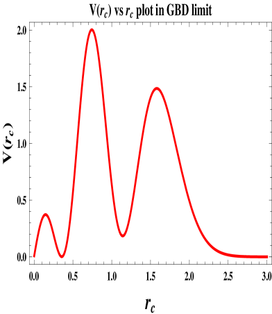
(a) $L=10^{-7},S=0.09,\frac{{\cal V}_{h}}{{\cal V}_{v}}=1.25$

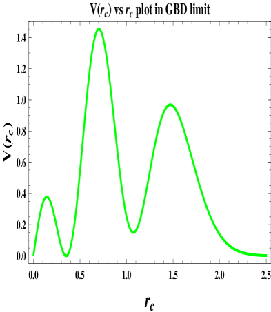
(b) $L=10^{-1},S=0.09,\frac{{\cal V}_{h}}{{\cal V}_{v}}=1.25$

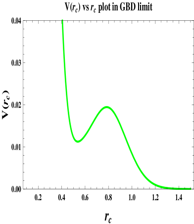
(c) $L=0.78,S=0.09,\frac{{\cal V}_{h}}{{\cal V}_{v}}=1.25$

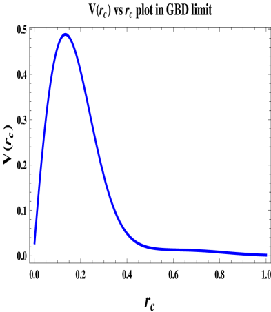
(d) $L=0.92,S=0.09,\frac{{\cal V}_{h}}{{\cal V}_{v}}=1.25$

Figure 1: Behaviour of the moduli stabilized potential with respect to the compactification radius $r_{c}$ in Gauss Bonnet dilaton (GBD) limit.

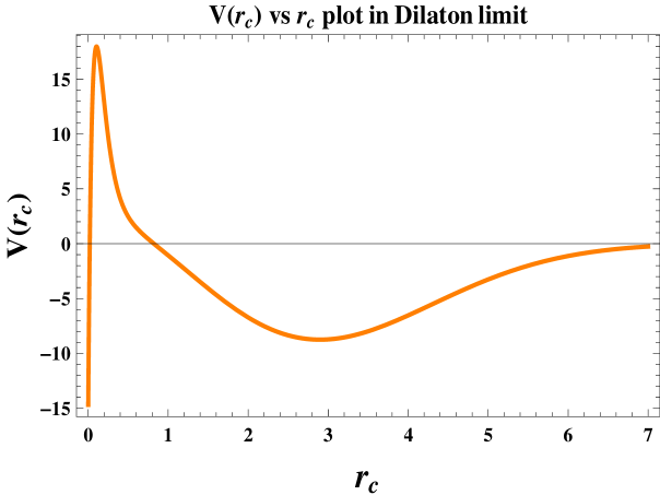
(a) $L=0,S=50,\frac{{\cal V}_{h}}{{\cal V}_{v}}=1.25$

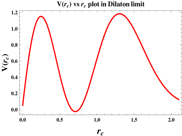
(b) $L=0,S=0.4,\frac{{\cal V}_{h}}{{\cal V}_{v}}=1.25$

Figure 2: Behaviour of the modulus potential with respect to the compactification radius $r_{c}$ in pure dilaton limit.

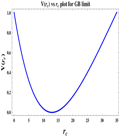
(a) $L=4\times 10^{-7},S=0,\frac{{\cal V}_{h}}{{\cal V}_{v}}=1.5$

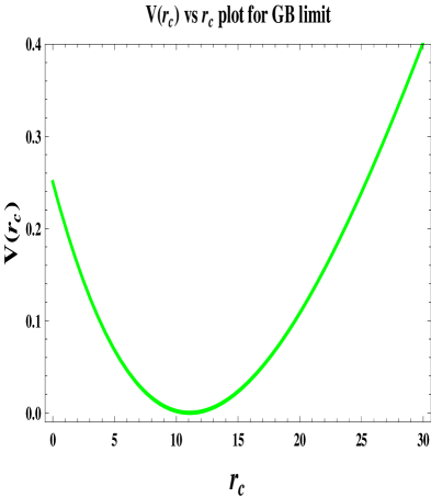
(b) $L=10^{-1},S=0,\frac{{\cal V}_{h}}{{\cal V}_{v}}=1.25$

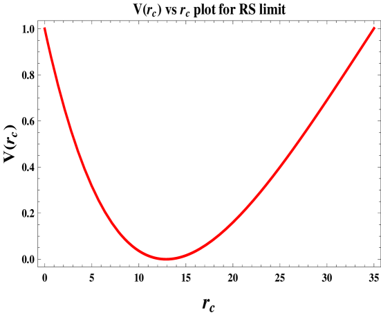
(c) $L=0,S=0,\frac{{\cal V}_{h}}{{\cal V}_{v}}=1.5$

Figure 3: Behaviour of the modulus potential with respect to the compactification radius $r_{c}$ for Einstein-GB-dilaton gravity.

3 Features of the stabilized potential in higher curvature gravity

Different	L	S	$\frac{{\cal V}_{h}}{{\cal V}_{v}}$	existence of		value of $r_{c}$		value of Potential$V(r_{c})$
features				$minima$	$Maxima$	$minima$	$maxima$	$minima$	$maxima$
Gauss-Bonnet	$10^{-7}$	0.09	1.25	double	double	0.3465,1.14	0.7379,1.573	0.004842,0.1855	2.013,1.491
Dilaton	$10^{-1}$	0.09	1.25	double	double	0.3461,1.07	0.7031, 1.495	0.003442,0.1441	7.421, 3.621
(GBD limit)	$0.78$	0.09	1.25	Single	X	0.4975	X	0.01214	X
	$0.92$	0.09	1.25	X	Single	X	0.1281	X	0.4865
Dilaton limit	0	50	1.25	Single	single	2.873	0.1019	-8.719	17.79
	0	0.4	1.25	Single	double	0.7119	0.2496, 1.312	-0.01827	1.156, 1.192
GB limit	$4\times 10^{-7}$	0	1.5	minima	X	12.77	X	-0.002217	X
	$10^{-1}$	0	1.25	minima	X	11.19	X	-0.001096	X
RS limit	0	0	1.5	minima	X	12.74	X	-0.00067	X

Table 1: Values of moduli radius and moduli potential in GBD, dilaton limit, GB and RS limit.

3.1 Case I: Einstein-Gauss Bonnet-dilaton bulk $(\alpha_{5}\neq 0,c_{1}\neq 0)$:

It is clear from the table (1), fig (1(a)) and fig (1(b)) that in this case there exists multiple (double) number of minima of the modulus potential obtained from the stabilization condition of modulus within the interval, $10^{-1}\leq L\leq 10^{-7}$ for fixed dilaton coupling at $S\sim 0.09$. In fig (1(a)) and fig (1(b)), the first minima appears to be more stable than the second one. The presence of more than one minimum implies the possibility of tunneling from one minimum to a more stable one i.e.the one with a lesser value of the moduli potential $V(r_{c})$. From the table (1) it may be seen that this causes decrease in the value of rc. For a given ${\cal V}_{h}/{\cal V}_{v}$, this will result into an increase in the value of the warp factor causing an enhancement of the value of the graviton Kaluza Klien (KK) mode masses and decrease in the value of the KK graviton coupling to brane fields. As a result the cross section for the KK graviton exchange will fall.Though the presence of two minima may imply the possibility of tunneling, however as the two minima are separated by a width ${\cal O}(M_{p})$ one can rule out the possibility of tunneling from one stabilized minimum to the adjacent one. We also observe from our analysis that if one increases the ratio of VEV, then the position of the minimum of the potential slightly shifts toward the higher value of the $r_{c}$. We have seen that as the strength of the GB coupling increases, one passes from double minima to single minimum. Most significantly, the increase in GB coupling causes the minima to disappear while a maximum appears in the moduli potential.This signals disappearance of any stable value for the modulus implying that large GB coupling leads to instability. See fig (1(d)) for details. Moreover it can be seen that as the VEV decreases (ratio becomes $\sim 1.25$), the potential becomes deeper implying greater stability. Additionally, for $L=0.78,S=0.09$ and $L=0.92,S=0.09$ we get one minimum and one maximum respectively as shown in fig (1(c)-1(d)). Also we observe that when $L$ changes from $10^{-7}$ to $10^{-1}$, for $S\sim 0.2-0.9$ we get double minima of the potential. As $S$ increases from 0.9 the double minima disappears and we have single minimum. On the other hand, if $S$ decreases from 0.2, at about $S\sim 0.014$, we have an appearance of single minimum in the modulus potential.We always keep $L$ from $10^{-7}$ to $10^{-1}$ since $L\geq 1$ is not a feasible value as the perturbative setup will no longer be valid and the theory goes to the non-perturbative regime of the solution which is beyond the scope of the present analysis.

3.2 Case II: Dilaton limit $(\alpha_{5}=0,c_{1}\neq 0)$:

If one considers the dilaton limit, then from the table (1), one single minimum is observed. In fig (2(a)) and fig (2(b)) we have depicted such features of stabilized potential with respect to modulus for the weak and strong dilaton coupling fixed at $S=0.4$ and $S=50$ respectively. We also observe from the present analysis that as in case of GBD scenario no such double minima appears in the scenario where only dilaton coupling is present. Moreover as the strength of the dilaton coupling increases, stability of the effective potential decreases.

3.3 Case III: Gauss-Bonnet limit $(\alpha_{5}\neq 0,c_{1}=0)$:

In GB limit, only single minimum is observed as mentioned in table (1). The behaviour of the modulus potential is depicted in fig (3(a)) for the ratio of the VEV$\sim 1.5$. Here we choose the value of the GB coupling $\sim{\cal O}(10^{-7})$ as constrained by various collider (i.e. higgs mass, $H\rightarrow\gamma\gamma,\tau\bar{\tau}$ decay [56] obtained from ATLAS [75, 76, 77] and CMS data [78]) and solar system observations [79]. There is no known dynamical origin of the small value of the Gauss-Bonnet coupling ${\cal O}(10^{−7})$. The consistency of the experimental results points towards this value. We have analyzed that as the VEV decreases (ratio becomes $\sim 1.25$) for a fixed GB coupling, the position of the minimum gets closer to the origin. By adjusting the GB parameter $L$ , we can address the well known hierarchy problem. For example, initially the ratio of VEV is fixed at $1.5$. In such a case $k_{L}r_{c}\sim{\cal O}(12.77)$ through which one can solve the hierarchy problem even in the weak GB coupling $\sim{\cal O}(10^{-7})$. Now if the ratio of the VEV is decreased to $1.25$ then we observe that $k_{L}r_{c}\sim{\cal O}(6.98)$, which implies that fine tuning problem cannot be addressed with a very weak GB coupling $\sim{\cal O}(10^{-7})$. But if we increase the GB coupling to $\sim{\cal O}(10^{-1})$ within the perturbative regime then even with the decreased value of the ratio of VEV to $1.25$ the gauge hierarchy problem can be addressed. See fig (3(b)) for the details. Using the Eq (2.23) we find that the ratio of the VEV can be expressed in the GB limit as:

$$\frac{{\cal V}_{h}}{{\cal V}_{v}}=e^{\frac{\pi r_{c}m_{\phi}^{2}}{4k_{RS}(1+L)}}.$$ (3.1)

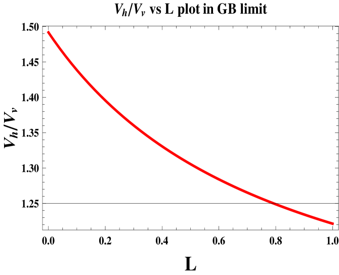
Figure 4: Variation of the ratio of VEV with respect to the GB parameter $L$ for $\frac{\pi r_{c}m_{\phi}^{2}}{4k_{RS}}\sim\frac{2}{5}$.

The variation of the ratio of VEV is given with respect to the GB parameter $L$ in Fig (4).From this figure, it can be clearly seen that in the limit $L\rightarrow 0$,we retrieve the RS limit. Thus we can generate a parameter space consisting of the GB coupling and ratio of the VEV to resolve the hierarchy problem.

Recently, in the context of radion phenomenology,[80] it has been shown that in the presence of GB coupling, radion VEV can be consistently adjusted to give first graviton excitation mass well above $\sim$ $3$ TeV as required from the latest ATLAS data.

3.4 Case IV: Randall-Sundrum limit $(\alpha_{5}=0,c_{1}=0)$:

In the RS limit, single minimum has been observed as mentioned in table (1) The behaviour of the moduli potential is depicted in fig (3(c)) for the ratio of the VEV $\sim 1.5$. To resolve the hierarchy problem, one should fix the ratio to this prescribed value. If the ratio of the VEV decreases( ratio becomes $\sim 1.25$) , the position of the minimum gets closer to the origin and stability of the effective moduli potential increases. However unlike the previous case now we have no parameter like GB parameter to the value of $k_{RS}r_{c}$ so that a Planck to TeV scale warping can be achieved. Hence, we can conclude that in case of zero GB coupling and zero dialton coupling, we have a specific choice for the ratio of the VEVs of the bulk scalar to address the hierarchy issue. The presence of GB and dilaton in the bulk provide us with flexibility in this choice.

4 Conclusion

In this work, we have studied the modulus stabilization mechanism in warped braneworld model when higher curvature gravity is present in the bulk via GB and dilaton coupling (GBD). We have also studied different limiting situations such as pure GB limit, pure dilaton limit and the RS limit. Analytical expressions for the stabilized potentials are derived for different cases. We summarize our results as follows:

• We observe the existence of double minima when both GB and dilaton coupling are present. As the strength of the GB coupling increases the unstable minimum of these two double minima disappears, resulting into a single minimum. If we go on increasing the strength of the GB coupling then it is observed that the single minimum disappears and a single maximum in the modulus potential appears. Thus increasing the GB coupling beyond a value leads to instability. Hence, in the perturbative regime of the solution we can always obtain a stabilized modulus potential although these stabilized values of the modulus radius $r_{c}$ are not effective in resolving the gauge hierarchy or fine-tuning problem as $k_{\bf M}r_{c}<<{\cal O}(12)$. We observe that as $S$ goes beyond the value $\sim 0.9$ the minimum of the potential disappears and we move to the region of instability. On the other hand, if value of the dilaton coupling decreases from a value $\sim 0.2$ we have appearance of single minimum.

• The existence of double minima of the moduli potential in higher curvature gravity may have interesting consequences in the context of stability of the model. As the minima in GBD case are separated by a width ${\cal O}(M_{p})$ one can rule out the possibility of tunneling from one stabilized minimum to the adjacent one.

• In case of pure dilaton limit we observe that as the strength of the dilaton coupling increases the stability of the effective moduli potential increases. Also we have only one minimum of the potential in this case.

• In case of pure GB limit also only single minimum is observed. For a fixed weak GB coupling, as the ratio of the VEV decreases, position of the minimum gets closer to the origin. It is also observed that using weak GB coupling and large ratio of VEV one cannot solve the hierarchy issue. However in the GB limit we observe that if the value of the GB coupling is increased then by decreasing the ratio of VEV it is still possible to resolve the gauge hierarchy problem.

• In the RS limit single minimum is observed as found in GW mechanism. One can solve the fine-tuning problem by taking a small value of the ratio of the VEV.

• It is well known that in RS model the various KK graviton modes are important sources for phenomenological signatures. The possible diphoton/dilepton decay channel of such gravitons are being studied by ATLAS collaboration in LHC. The most recent result has set stringent lower bounds on the 1st KK graviton $\sim 3$ TeV [68]. With pure Einstein gravity in the bulk it is very difficult to satisfy this bound and it has been demonstrated that the presence of higher curvature terms along with dilaton can explain the ATLAS result. In this context the study of stability of our proposed model is of utmost importance. Through this work we therefore undertake to present a detailed analysis of stabilizing the higher curvature modified warped geometry model in presence of dilaton.

In summary, if we compare our findings with the original Goldberger-Wise stabilization mechanism we observe that the presence of Gauss-Bonnet (GB) higher curvature term and dilaton term produces the following modification in the modulus stabilization scenario.

• If GB coupling $L$ increases beyond a desired value, for a given dilaton coupling $S$, then the minima of the potential disappears.
  

• The value of the dilaton coupling $S$ should be below a critical value to avoid the appearance of double minima which removes the possibility of tunneling.
  

• The reduction in the stabilized value of the modulus $r_{c}$ (Please see the Table 1) than Goldberger-Wise scenario implies an improvement in reducing the hierarchy between $r_{c}$ and inverse of the 4D Planck scale $M^{-1}_{pl}$.

5 Appendix

Let us explicitly write down the expression for the stabilized potential for the modulus in case of Gauss-Bonnet dilaton:

$$\begin{array}[]{lllll}V_{\Phi}(r_{c})=V_{1}(r_{c})+V_{2}(r_{c}),\end{array}$$ (5.1)

where for Gauss-Bonnet dilaton gravity $V_{1}(r_{c})$ and $V_{2}(r_{c})$ are given by the following expressions:

$$\small\begin{array}[]{llll}V_{1}(r_{c})=-\frac{1}{\Gamma[(1+A/4)^{2}]}M_{1}(-1/(Z_{L}^{5}Q^{5})e^{-Z_{L}BQ^{2}}\\ ~{}~{}~{}~{}~{}~{}~{}~{}~{}~{}~{}~{}~{}~{}(-M^{2}(6A^{2}+6Z_{L}BQ^{2}A^{2}+2Z^{3}_{L}BQ^{4}A(1+B^{2}Q^{2}A/2)+Z^{4}_{L}Q^{4}(1+B^{2}Q^{2}A/2)^{2}\\ ~{}~{}~{}~{}+2Z^{2}_{L}Q^{2}A(1+3B^{2}Q^{2}A/2))\Gamma(1+A/4)^{2}-Z_{L}^{2}M^{2}Q^{2}(2+Z_{L}^{2}B^{2}Q^{4}+2Z_{L}BQ^{2})A^{2}\Gamma[(1+A/2)/2]^{2}\\ ~{}~{}~{}~{}~{}~{}~{}~{}~{}~{}~{}~{}~{}~{}~{}~{}~{}~{}+Z_{L}MQA(6A+6Z_{L}BQ^{2}A+Z_{L}^{3}BQ^{4}(1+B^{2}Q^{2}A)\\ ~{}~{}~{}~{}~{}~{}~{}~{}~{}~{}~{}~{}~{}~{}~{}~{}~{}+Z_{L}^{2}Q^{2}(1+3B^{2}Q^{2}A))W\Gamma[(1+A/2)/2]\Gamma[(1+A/2)]\\ ~{}~{}~{}~{}~{}~{}~{}~{}~{}~{}-(24A^{2}+24Z_{L}BQ^{2}A^{2}+4Z_{L}^{3}BQ^{4}A(1+B^{2}Q^{2}A)+Z_{L}^{4}Q^{4}(1+B^{2}Q^{2}A)^{2}\\ ~{}~{}~{}~{}~{}~{}~{}~{}~{}~{}~{}~{}+4Z_{L}^{2}Q^{2}A(1+3B^{2}Q^{2}A))W^{2}\Gamma[(1+A/2)^{2}]\\ ~{}~{}~{}~{}~{}~{}~{}~{}+2M\Gamma[(1+A/4)](Z_{L}MQA/2(3A+3Z_{L}BQ^{2}A+Z_{L}^{3}BQ^{4}(1+B^{2}Q^{2}A/2)\\ ~{}~{}~{}~{}~{}~{}~{}~{}+Z_{L}^{2}Q^{2}(1+3B^{2}Q^{2}A/2))\Gamma[(1+A/2)/2]--(12A^{2}+12Z_{L}BQ^{2}A^{2}+3Z_{L}^{2}Q^{2}A(1+2B^{2}Q^{2}A)\\ ~{}~{}~{}~{}~{}~{}~{}+Z_{L}^{3}BQ^{4}A(3+2B^{2}Q^{2}A)+Z_{L}^{4}Q^{4}(1+3B^{2}Q^{2}A/2+B^{4}Q^{4}A^{2}/2))W\Gamma[(1+A/2)]))\\ ~{}~{}~{}~{}~{}~{}~{}+1/(Z_{L}^{5}Q^{5})e^{-Z_{L}BQ(Q+\pi S)}(-M^{2}(6A^{2}+6Z_{L}BQ(Q+\pi S)A^{2}\\ ~{}~{}~{}~{}~{}~{}~{}~{}~{}+2z^{3}BQ^{3}(Q+\pi S)A(1+B^{2}(Q+\pi S)^{2}A/2)+z^{4}Q^{4}(1+B^{2}(Q+\pi S)^{2}A/2)^{2}\\ ~{}~{}~{}~{}~{}~{}~{}~{}~{}+2z^{2}Q^{2}A(1+3B^{2}(Q+\pi S)^{2}A/2))\Gamma(1+A/4)^{2}-(Z_{L}^{2}M^{2}Q^{2}/4)(2+2Z_{L}BQ(Q+\pi S)\\ ~{}~{}~{}~{}~{}~{}~{}~{}+Z_{L}^{2}B^{2}Q^{2}(Q+\pi S))A^{2}\Gamma[(1+A/2)/2]^{2}+Z_{L}MQA(6A+6Z_{L}BQ(Q+\pi S)A\\ ~{}~{}~{}~{}~{}~{}~{}~{}~{}~{}+Z_{L}^{3}BQ^{3}(Q+\pi S)(1+B^{2}(Q+\pi S)^{2}A/2)\\ ~{}~{}~{}~{}~{}~{}~{}~{}~{}+Z_{L}^{2}Q^{2}(1+3B^{2}(Q+\pi S)^{2}A/2))W\Gamma[(1+A/2)/2]\Gamma[(1+A/2)]\\ ~{}~{}~{}~{}~{}~{}~{}-(24A^{2}+24Z_{L}BQ(Q+\pi S)A^{2}+4Z_{L}^{3}BQ^{3}(Q+\pi S)A(1+B^{2}(Q+\pi S)^{2}A)\\ ~{}~{}~{}~{}~{}~{}~{}~{}~{}~{}~{}~{}+Z_{L}^{4}Q^{4}(1+B^{2}(Q+\pi S)^{2}A)^{2}+4Z_{L}^{2}Q^{2}A(1+3B^{2}(Q+\pi S)^{2}A))W^{2}\Gamma[(1+A/2)^{2}]\\ ~{}~{}~{}~{}~{}~{}~{}~{}~{}~{}~{}~{}~{}~{}~{}~{}~{}~{}+2M\Gamma[(1+A/4)](Z_{L}MQA/2(3A+3Z_{L}BQ(Q+\pi S)A\\ ~{}~{}~{}~{}+Z_{L}^{3}BQ^{3}(Q+\pi S)(1+B^{2}(Q+\pi S)^{2}A/2)+Z_{L}^{2}Q^{2}(1+3B^{2}(Q+\pi S)^{2}A/2))\Gamma[(1+A/2)/2]-\\ ~{}~{}~{}~{}~{}~{}~{}~{}-(12A^{2}+12Z_{L}BQ(Q+\pi S)A^{2}+3Z_{L}^{2}Q^{2}A(1+2B^{2}(Q+\pi S)^{2}A)\\ ~{}~{}~{}~{}~{}~{}~{}~{}~{}~{}+Z_{L}^{3}BQ^{3}(Q+\pi S)A(3+2B^{2}(Q+\pi S)^{2}A)+Z_{L}^{4}Q^{4}(1+3B^{2}(Q+\pi S)^{2}A/2\\ ~{}~{}~{}~{}~{}~{}~{}~{}~{}~{}~{}~{}+B^{4}(Q+\pi S)^{4}A^{2}/2))W\Gamma[(1+A/2)])))\end{array}$$ (5.2)

$$\small\begin{array}[]{llll}V_{2}(r_{c})=-\frac{1}{\Gamma[(1+A/2)]^{2}}Z_{L}SA(e^{-Z_{L}BQ^{2}}(-\frac{1}{4S}QA(-4M\Gamma[(1+A/4)]+3Z_{L}MQ\Gamma[(1+A/2)/2]\\ ~{}~{}~{}~{}~{}~{}~{}~{}~{}~{}~{}~{}-8W\Gamma[(1+A/2)](M\Gamma[(1+A/4)]+2W\Gamma[(1+A/2)])+B^{3}Q^{3}A(M\Gamma[(1+A/4)]\\ ~{}~{}~{}~{}~{}~{}~{}~{}~{}~{}~{}~{}+2W\Gamma[(1+A/2)])^{2}-\frac{1}{Z_{L}^{3}Q^{3}}(-4M^{2}A\Gamma[(1+A/4)]^{2}-Z_{L}^{2}M^{2}Q^{2}A/2\Gamma[(1+A/2)/2]^{2}\\ ~{}~{}~{}~{}~{}~{}~{}~{}~{}~{}~{}~{}~{}+Z_{L}MQ(Z_{L}^{2}Q^{2}+4A)W\Gamma[(1+A/2)/2]\Gamma[1+(A/2)]-16AW^{2}\Gamma[1+(A/2)]^{2}\\ ~{}~{}~{}~{}~{}~{}~{}~{}~{}~{}~{}~{}+M\Gamma[(1+A/4)](Z_{L}MQ(Z_{L}^{2}Q^{2}+2A)\Gamma[(1+A/2)/2]-16AW\Gamma[1+(A/2)]))\\ ~{}~{}~{}~{}~{}~{}~{}~{}~{}~{}~{}~{}+\frac{1}{2Z_{L}BQS}(2M^{2}(Z_{L}^{2}Q^{2}+2A)\Gamma[(1+A/4)]^{2}+Z_{L}^{2}M^{2}Q^{2}A/2\Gamma[1+(A/2)]^{2}\\ ~{}~{}~{}~{}~{}~{}~{}~{}~{}~{}~{}-4Z_{L}MQAW\Gamma[(1+(A/2)/2)]\Gamma[1+(A/2)]+4(Z_{L}^{2}Q^{2}+4A)W^{2}\Gamma[1+(A/2)]^{2}\\ ~{}~{}~{}~{}~{}~{}~{}~{}~{}~{}~{}~{}~{}+2M\Gamma[(1+A/4)](-Z_{L}MQA\Gamma[(1+(A/2)/2)]+(3Z_{L}^{2}Q^{2}+8A)W\Gamma[(1+(A/2))])))\\ ~{}~{}~{}~{}~{}~{}~{}~{}~{}~{}~{}~{}+e^{-Z_{L}BQ(Q+\pi S)}(\frac{1}{4QS}(Q+\pi S)^{2}A(-4M\Gamma[(1+A/4)]\\ ~{}~{}~{}~{}~{}~{}~{}~{}~{}~{}~{}+3Z_{L}MQ\Gamma[(1+A/2)/2]-8W\Gamma[(1+A/2)])(M\Gamma[(1+A/4)]+2W\Gamma[(1+A/2)])\\ ~{}~{}~{}~{}~{}~{}~{}~{}~{}~{}~{}~{}-B^{3}(Q+\pi S)^{3}A(M\Gamma[(1+A/4)]+2W\Gamma[(1+A/2)])^{2}\\ ~{}~{}~{}~{}~{}~{}~{}~{}~{}~{}~{}~{}+\frac{1}{Z_{L}^{3}Q^{3}}(-4M^{2}A\Gamma[(1+A/4)]^{2}-(Z_{L}^{2}M^{2}Q^{2}A/2)\Gamma[(1+A/2)/2]^{2}\\ ~{}~{}~{}~{}~{}~{}~{}~{}~{}~{}~{}~{}+Z_{L}MQ(Z_{L}^{2}Q^{2}+4A)W\Gamma[(1+A/2)/2]\Gamma[1+(A/2)]-16AW^{2}\Gamma[1+(A/2)]^{2}\\ ~{}~{}~{}~{}~{}~{}~{}~{}~{}~{}~{}~{}+M\Gamma[(1+A/4)](Z_{L}MQ(Z_{L}^{2}Q^{2}+2A)\Gamma[(1+A/2)/2]-16AW\Gamma[1+(A/2)]))\\ ~{}~{}~{}~{}~{}~{}~{}~{}~{}~{}~{}~{}~{}-\frac{1}{2Z_{L}BQ^{2}S}(Q+\pi S)(2M^{2}(Z_{L}^{2}Q^{2}+2A)\Gamma[(1+A/4)]^{2}+Z_{L}^{2}M^{2}Q^{2}A/2\Gamma[(1+(A/2))/2]^{2}\\ ~{}~{}~{}~{}~{}~{}~{}~{}~{}~{}~{}-4Z_{L}MQAW\Gamma[(1+(A/2)/2)]\Gamma[1+(A/2)]+4(Z_{L}^{2}Q^{2}+4A)W^{2}\Gamma[1+(A/2)]^{2}\\ ~{}~{}~{}~{}~{}~{}~{}~{}~{}~{}~{}~{}~{}+2M\Gamma[(1+A/4)](-Z_{L}MQA\Gamma[(1+(A/2)/2)]+(3Z_{L}^{2}Q^{2}+8A)W\Gamma[(1+(A/2))]))))\end{array}$$ (5.3)

where all the parameters $Q,S,L,Z_{L},A,B$ are deined in Eq (2.14) and Eq (2.17). Further if we substitute $Z_{L}=1$ in Eq (5.1), Eq (5.2) and Eq (5.3) then it results in the stabilized potential for modulus in case of pure dilaton gravity limit as mentioned in 2.4.3.

References

- [1] M. Berg, M. Haack and B. Kors, JHEP 0511 (2005) 030 [hep-th/0508043].
- [2] M. Cicoli, J. P. Conlon and F. Quevedo, JHEP 0801 (2008) 052 [arXiv:0708.1873 [hep-th]].
- [3] M. A. Bershadsky, Mod. Phys. Lett. A 3 (1988) 91.
- [4] Z. Kakushadze and T. R. Taylor, Nucl. Phys. B 562 (1999) 78 [hep-th/9905137].
- [5] M. B. Green, H. -h. Kwon and P. Vanhove, Phys. Rev. D 61 (2000) 104010 [hep-th/9910055].
- [6] R. Roiban, A. Tirziu and A. A. Tseytlin, JHEP 0707 (2007) 056 [arXiv:0704.3638 [hep-th]].
- [7] H. P. Nilles, Phys. Rept. 110 (1984) 1.
- [8] D. H. Lyth and A. Riotto, Phys. Rept. 314 (1999) 1 [hep-ph/9807278].
- [9] P. Van Nieuwenhuizen, Phys. Rept. 68 (1981) 189.
- [10] A. Mazumdar and J. Rocher, Phys. Rept. 497 (2011) 85 [arXiv:1001.0993 [hep-ph]].
- [11] D. Z. Freedman, P. van Nieuwenhuizen and S. Ferrara, Phys. Rev. D 13 (1976) 3214.
- [12] S. Choudhury, A. Mazumdar and E. Pukartas, JHEP 1404 (2014) 077 [arXiv:1402.1227 [hep-th]].
- [13] S. Choudhury, JHEP 04 (2014) 105 [arXiv:1402.1251 [hep-th]].
- [14] S. Choudhury, A. Mazumdar and S. Pal, JCAP 1307 (2013) 041 [arXiv:1305.6398 [hep-ph]].
- [15] S. Choudhury, T. Chakraborty and S. Pal, Nucl. Phys. B 880 (2014) 155 [arXiv:1305.0981 [hep-th]].
- [16] S. Choudhury and S. Pal, J. Phys. Conf. Ser. 405 (2012) 012009 [arXiv:1209.5883 [hep-th]].
- [17] S. Choudhury and S. Pal, Phys. Rev. D 85 (2012) 043529 [arXiv:1102.4206 [hep-th]].
- [18] S. Choudhury and S. Pal, Nucl. Phys. B 857 (2012) 85 [arXiv:1108.5676 [hep-ph]].
- [19] Superstring Theory. Vol. 1: Introduction - Green, Michael B. et al. Cambridge, Uk: Univ. Pr. ( 1987) 469 P. ( Cambridge Monographs On Mathematical Physics).
- [20] Superstring Theory. Vol. 2: Loop Amplitudes, Anomalies And Phenomenology - Green, Michael B. et al. Cambridge, Uk: Univ. Pr. ( 1987) 596 P. ( Cambridge Monographs On Mathematical Physics).
- [21] String theory. Vol. 1: An introduction to the bosonic string - Polchinski, J. Cambridge, UK: Univ. Pr. (1998) 402 p.
- [22] String theory. Vol. 2: Superstring theory and beyond - Polchinski, J. Cambridge, UK: Univ. Pr. (1998) 531 p.
- [23] M. Evans and B. A. Ovrut, Phys. Lett. B 171 (1986) 177.
- [24] T. D. Robb and J. G. Taylor, Phys. Lett. B 176 (1986) 355.
- [25] D. J. Gross, J. A. Harvey, E. J. Martinec and R. Rohm, Nucl. Phys. B 267 (1986) 75.
- [26] P. Candelas, M. D. Freeman, C. N. Pope, M. F. Sohnius and K. S. Stelle, Phys. Lett. B 177 (1986) 341.
- [27] Y. Cai and C. A. Nunez, Nucl. Phys. B 287 (1987) 279.
- [28] W. D. Goldberger and M. B. Wise, Phys. Rev. Lett. 83 (1999) 4922 [hep-ph/9907447].
- [29] W. D. Goldberger and M. B. Wise, Phys. Lett. B 475 (2000) 275 [hep-ph/9911457].
- [30] W. D. Goldberger and M. B. Wise, Phys. Rev. D 60 (1999) 107505 [hep-ph/9907218].
- [31] O. DeWolfe, D. Z. Freedman, S. S. Gubser and A. Karch, Phys. Rev. D 62 (2000) 046008 [hep-th/9909134].
- [32] A. Dey, D. Maity and S. SenGupta, Phys. Rev. D 75 (2007) 107901 [hep-th/0611262].
- [33] S. Das, A. Dey and S. SenGupta, Europhys. Lett. 83 (2008) 51002 [arXiv:0704.3119 [hep-th]].
- [34] A. Das, S. Kar and S. SenGupta, Int. J. Mod. Phys. A 24 (2009) [arXiv:0804.1757 [hep-th]].
- [35] D. Maity, S. SenGupta and S. Sur, Class. Quant. Grav. 26 (2009) 055003 [hep-th/0609171].
- [36] Z. Chacko and A. E. Nelson, Phys. Rev. D 62 (2000) 085006 [hep-th/9912186]
- [37] E. Ponton and E. Poppitz, JHEP 0106 (2001) 019 [hep-ph/0105021].
- [38] C. Charmousis and U. Ellwanger, JHEP 0402 (2004) 058 [hep-th/0402019].
- [39] C. P. Burgess, D. Hoover and G. Tasinato, JHEP 0709 (2007) 124 [arXiv:0705.3212 [hep-th]].
- [40] J. M. Cline and H. Firouzjahi, Phys. Rev. D 64 (2001) 023505 [hep-ph/0005235].
- [41] P. Kanti, I. I. Kogan, K. A. Olive and M. Pospelov, Phys. Rev. D 61 (2000) 106004 [hep-ph/9912266].
- [42] P. Binetruy, J. M. Cline and C. Grojean, Phys. Lett. B 489 (2000) 403 [hep-th/0007029].
- [43] P. R. Ashcroft, C. van de Bruck and A. -C. Davis, Phys. Rev. D 71 (2005) 023508 [astro-ph/0408448].
- [44] K. Ghoroku and A. Nakamura, Phys. Rev. D 64 (2001) 084028 [hep-th/0103071].
- [45] A. Lewandowski and R. Sundrum, Phys. Rev. D 65 (2002) 044003 [hep-th/0108025].
- [46] J. Lesgourgues and L. Sorbo, Phys. Rev. D 69 (2004) 084010 [hep-th/0310007].
- [47] T. Kobayashi and K. Yoshioka, JHEP 0411 (2004) 024 [hep-ph/0409355].
- [48] M. Eto, N. Maru and N. Sakai, Phys. Rev. D 70 (2004) 086002 [hep-th/0403009].
- [49] I. H. Brevik, K. Ghoroku and M. Yahiro, Phys. Rev. D 70 (2004) 064012 [hep-th/0402176].
- [50] N. J. Nunes and M. Peloso, Phys. Lett. B 623 (2005) 147 [hep-th/0506039].
- [51] S. Ichinose and A. Murayama, Phys. Lett. B 625 (2005) 106 [hep-th/0409193].
- [52] F. Brummer, A. Hebecker and E. Trincherini, Nucl. Phys. B 738 (2006) 283 [hep-th/0510113].
- [53] S. Choudhury and S. Pal, Nucl. Phys. B 874 (2013) 85 [arXiv:1208.4433 [hep-th]].
- [54] S. Choudhury and S. Pal, arXiv:1210.4478 [hep-th].
- [55] S. Choudhury and A. Dasgupta, Nucl. Phys. B 882 (2014) 195 [arXiv:1309.1934 [hep-ph]].
- [56] S. Choudhury, S. Sadhukhan and S. SenGupta, arXiv:1308.1477 [hep-ph].
- [57] S. Choudhury and S. SenGupta, arXiv:1306.0492 [hep-th].
- [58] S. Choudhury and S. SenGupta, JHEP 1302 (2013) 136 [arXiv:1301.0918 [hep-th]].
- [59] S. Choudhury and S. SenGupta, arXiv:1311.0730 [hep-ph].
- [60] J. E. Kim, B. Kyae and H. M. Lee, Phys. Rev. D 62 (2000) 045013 [hep-ph/9912344].
- [61] H. M. Lee, hep-th/0010193.
- [62] J. E. Kim, B. Kyae and H. M. Lee, Nucl. Phys. B 582 (2000) 296 [Erratum-ibid. B 591 (2000) 587] [hep-th/0004005].
- [63] J. E. Kim and H. M. Lee, Nucl. Phys. B 602 (2001) 346 [Erratum-ibid. B 619 (2001) 763] [hep-th/0010093].
- [64] L. Randall and R. Sundrum, Phys. Rev. Lett. 83 (1999) 3370 [hep-ph/9905221].
- [65] L. Randall and R. Sundrum, Phys. Rev. Lett. 83 (1999) 4690 [hep-th/9906064].
- [66] M. Reece and L. -T. Wang, JHEP 1007 (2010) 040 [arXiv:1003.5669 [hep-ph]].
- [67] H. Davoudiasl, J. L. Hewett and T. G. Rizzo, Phys. Rev. Lett. 84 (2000) 2080 [hep-ph/9909255].
- [68] A. Das and S. SenGupta, arXiv:1303.2512 [hep-ph].
- [69] R. Koley, J. Mitra and S. SenGupta, Europhys. Lett. 91 (2010) 31001 [arXiv:1001.2666 [hep-th]].
- [70] T. G. Rizzo, JHEP 0501 (2005) 028 [hep-ph/0412087].
- [71] G. Dotti, J. Oliva and R. Troncoso, Phys. Rev. D 76 (2007) 064038 [arXiv:0706.1830 [hep-th]].
- [72] T. Torii and H. Maeda, Phys. Rev. D 71 (2005) 124002 [hep-th/0504127].
- [73] R. A. Konoplya and A. Zhidenko, Phys. Rev. D 82 (2010) 084003 [arXiv:1004.3772 [hep-th]].
- [74] S. ’i. Nojiri and S. D. Odintsov, Phys. Rept. 505 (2011) 59 [arXiv:1011.0544 [gr-qc]].
- [75] [ATLAS Collaboration], ATLAS-CONF-2013-014.
- [76] G. Aad et al. [ATLAS Collaboration], Phys. Lett. B 716 (2012) 1 [arXiv:1207.7214 [hep-ex]].
- [77] G. Aad et al. [ATLAS Collaboration], Phys. Lett. B 710 (2012) 538 [arXiv:1112.2194 [hep-ex]].
- [78] S. Chatrchyan et al. [CMS Collaboration], JHEP 1306 (2013) 081 [arXiv:1303.4571 [hep-ex]].
- [79] S. Chakraborty and S. SenGupta, Phys. Rev. D 89 (2014) 026003 [arXiv:1208.1433 [gr-qc]].
- [80] U. Maitra, B. Mukhopadhyaya and S. SenGupta, arXiv:1307.3018.