Numerical simulations of quiet Sun magnetism: On the contribution from a small-scale dynamo

Abstract

We present a series of radiative MHD simulations addressing the origin and distribution of mixed polarity magnetic field in the solar photosphere. To this end we consider numerical simulations that cover the uppermost $2-6$ Mm of the solar convection zone and we explore scales ranging from $2$ km to $25$ Mm. We study how the strength and distribution of magnetic field in the photosphere and subsurface layers depend on resolution, domain size and boundary conditions. We find that $50\%$ of the magnetic energy at the $\tau=1$ level comes from field with the less than $500$ G strength and that $50\%$ of the energy resides on scales smaller than about $100$ km. While probability distribution functions are essentially independent of resolution, properly describing the spectral energy distribution requires grid spacings of $8$ km or smaller. The formation of flux concentrations in the photosphere exceeding $1$ kG requires a mean vertical field strength greater than $30-40$ G at $\tau=1$. The filling factor of kG flux concentrations increases with overall domain size as magnetic field becomes organized by larger, longer lived flow structures. A solution with a mean vertical field strength of around $85$ G at $\tau=1$ requires a subsurface RMS field strength increasing with depth at the same rate as the equipartition field strength. We consider this an upper limit for the quiet Sun field strength, which implies that most of the convection zone is magnetized close to equipartition. We discuss these findings in view of recent high-resolution spectropolarimetric observations of quiet Sun magnetism.

1. Introduction

Small-scale turbulent magnetic field is ubiquitous on the solar surface and provides the dominant contribution to the magnetic energy in the quiet Sun photosphere (see, e.g., Lites et al. (1996); Khomenko et al. (2003); Domínguez Cerdeña et al. (2003); Sánchez Almeida (2003); Trujillo Bueno et al. (2004); Domínguez Cerdeña et al. (2006); Orozco Suárez et al. (2007); Lites et al. (2008); Bellot Rubio & Orozco Suárez (2012) and recent reviews by de Wijn et al. (2009); Martínez Pillet (2013)). Several investigations found that inter-network magnetic field shows only little dependence on the solar cycle (Trujillo Bueno et al., 2004; Buehler et al., 2013) and also little correlation with the strength of the surrounding network field (Lites, 2011; Ishikawa & Tsuneta, 2009). This points toward an origin of the quiet Sun magnetic field largely independent from the global solar dynamo responsible for the solar cycle.

It was suggested by Petrovay & Szakaly (1993), based on a simplified transport model for signed and unsigned flux in the convection zone, that a small-scale dynamo is the key process maintaining turbulent magnetic field in the quiet Sun. Small-scale dynamos were first studied through MHD simulations in incompressible setups by Cattaneo (1999) and later with stratification (anelastic approximation) by Bercik et al. (2005). Vögler & Schüssler (2007) used the most ”solar-like” setup by including realistic physics in terms of equation of state and 3-dimensional radiative transfer. They were able to demonstrate that despite the lack of significant recirculation within the computational domain (use of open bottom boundary conditions that mimic the deep convection zone), a considerable amount of magnetic field can be maintained in the photosphere. It was found later that the photospheric field strength falls still short by a factor of $2-3$ compared to observations based on Zeeman diagnostics (Danilovic et al., 2010); an even more dramatic shortfall by about one order of magnitude was found by Shchukina & Trujillo Bueno (2011) based on Hanle-effect diagnostics. To which degree the discrepancy between the magnetic field strength found in solar photospheric dynamo simulations and observations is due to boundary conditions and resolution (which relates to the magnetic Reynolds numbers reached) is still an open issue, which we aim to adress primarily in this paper.

On a more fundamental level the operation as well as non-linear saturation of small-scale dynamos at very small magnetic Prandtl numbers ($P_{M}=\nu/\eta\ll 1$, with viscosity $\nu$ and magnetic diffusivity $\eta$) as encountered on the Sun ($P_{M}\sim 10^{-5}$) remains an open question. While the regime $P_{M}>1$ has been studied in great detail including the non-linear saturation phase (Schekochihin et al., 2004), the regime $P_{M}\ll 1$ is less accessible by direct numerical simulations. Small-scale dynamos at low $P_{M}$ were studied in the kinematic regime by Iskakov et al. (2007); Schekochihin et al. (2007) and in the non-linear regime by Brandenburg (2011). These investigations indicate that the threshold for dynamo action increases moderately when approaching the $P_{M}\ll 1$ regime, but small-scale dynamo action remains possible for large values of the magnetic Reynolds number typically found in astrophysical systems (Tobias et al., 2011; Brandenburg, 2011).

We present here an investigation which follows along the lines of comprehensive photospheric MHD simulations similar to the work presented by Vögler & Schüssler (2007); Pietarila Graham et al. (2010). In particular we address the problem that these simulations fall short by a factor of about $2-3$ in field strength when compared to observations as pointed out by Danilovic et al. (2010). We explore here the potential role of two factors: 1. Numerical resolution and magnetic diffusivities, 2. Influence from the bottom boundary condition. While numerical resolution and treatment of diffusivities determine the dynamo growth rate in the kinematic phase, $\gamma_{K}$, the bottom boundary condition determines the amount of magnetic energy that recirculates within the computational domain. It was first pointed out by Stein et al. (2003) that the rather small recirculation of plasma found in the top layers of the convection zone could be a major hurdle for a small-scale dynamo to exist locally in the photosphere. While the recirculation is small it is not zero, since some level of turbulent mixing between up- and downflow regions is unavoidable. Magnetic energy loss due to overturning convection happens on a rather slow time-scale $\sim H_{\varrho}/v_{z{\rm RMS}}$ (with density scale height $H_{\varrho}$ and vertical RMS velocity $v_{z{\rm RMS}}$), which can be compensated by a sufficiently efficient small-scale dynamo. Vögler & Schüssler (2007) showed that a local dynamo in the photosphere can operate despite small recirculation if the value of the magnetic diffusivity $\eta$ is smaller than $2.5\cdot 10^{10}\mbox{cm}^{2}\mbox{s}^{-1}$ (for a magnetic Prandtl number close to unity). Pietarila Graham et al. (2010) studied photospheric dynamos in the kinematic growth phase using values of $\eta$ as low as $4\cdot 10^{9}\mbox{cm}^{2}\mbox{s}^{-1}$, but did not study the non-linear saturation. The setup of Vögler & Schüssler (2007); Pietarila Graham et al. (2010) is conservative in terms of the bottom boundary condition. There is no vertical Poynting flux in upflow regions and in addition an enhanced magnetic diffusivity near the bottom boundary. Since it is likely that the bulk of the convection zone has strong magnetic field, it is reasonable to assume that upflow regions are magnetized and transport magnetic energy into the photosphere.

In order to adress these questions we consider models that differ from previous studies in the following aspects:
1. We use only numerical diffusivities in an attempt to minimize the influence from dissipation for a given numerical resolution. In comparison to direct numerical simulations (DNS) that use explicit diffusivities and fully resolve the dissipation range, our setup is more along the lines of large eddy simulations (LES) in which a high Reynolds number regime is realized on large scales, while the dissipation range is truncated through the use of a subgrid-scale model. In our case the latter is entirely based on monotonicity constraints through the use of a slope-limited diffusion scheme (see Section 2 for detail). This is an attempt to make the small-scale dynamo maximally efficient, i.e. to maximize the kinematic growth rate $\gamma_{K}$ for a given numerical resolution. This setup allows us to study a regime with strong non-linear feedback (saturated phase of the dynamo), but it does not allow us to address questions related to the magnetic Prandtl number (implicitly set by the numerical dissipation terms, in general close to unity).
2. We use generalized open boundary conditions which allow also for the presence of (mixed polarity) horizontal field in upflow regions. These are setups that explore a stronger coupling between the top layers (including photosphere) and the bulk of the convection zone. Formally these boundary conditions lead to different magnetic energy loss rates at the bottom boundary. While they do not strongly affect the kinematic growth phase of an efficient dynamo with $\gamma_{K}\gg v_{z{\rm RMS}}/H_{\varrho}$, they do become relevant in the non-linear saturation regime, which we primarily focus on here.
In addition we compare models with different resolutions as well as domain sizes to evaluate the robustness of results. Our aim is to investigate with this setup a small-scale dynamo operating in a regime that is consistent with observational constraints on the quiet Sun magnetic field strength, like those inferred by Danilovic et al. (2010). This regime is currently not accessible with comprehensive solar MHD simulations that use only physical diffusion terms (DNS) or even operate in a low $P_{M}$ regime.

The remainder of the paper is organized as follows: In Section 2 we describe in detail the numerical setup in terms of the equations solved, the formulation of numerical diffusivites, boundary conditions and domain sizes used. In Section 3 we present the results, subsections describe in detail the resolution dependence of results, the dependence on domain size and boundary conditions, and a detailed analysis of the dynamo process based on transfer functions in spectral space. In Section 4 we discuss our main findings in relation to observational constraints on quiet Sun magnetism, a detailed comparison with observations through forward modeling of spectral lines is deferred to future publications. Concluding remarks are presented in Section 5.

2. Numerical setup

2.1. Numerical scheme

We use for our simulations the MURaM radiative MHD code (Vögler et al., 2005; Rempel et al., 2009). This code uses a $4^{th}$ order accurate (in space and time) conservative, centered finite difference scheme for discretization of the MHD equations, combined with a short characteristics approach for radiative transfer. The code uses a tabulated OPAL equation of state (Rogers et al., 1996). We solve the MHD equations in the following form:

$$\frac{\partial\varrho}{\partial t} = -\nabla\cdot\left(\varrho\mathbf{v}\right)$$ (1)

$$\frac{\partial\varrho\mathbf{v}}{\partial t} = -\nabla\cdot(\varrho\mathbf{v}\mathbf{v})+\frac{f_{v_{A}}}{4\pi}\nabla\cdot\left(\mathbf{B}\mathbf{B}-\frac{1}{2}\mathbf{I}\,B^{2}\right)$$ (2)

$$-\nabla P+\varrho\mathbf{g}$$

$$\frac{\partial E_{\rm HD}}{\partial t} = -\nabla\cdot\left[\mathbf{v}\,(E_{\rm HD}+P)\right]+\varrho\mathbf{v}\cdot\mathbf{g}+\frac{\eta}{4\pi}(\nabla\times\mathbf{B})^{2}$$ (3)

$$+\mathbf{v}\cdot\frac{f_{v_{A}}}{4\pi}\nabla\cdot\left(\mathbf{B}\mathbf{B}-\frac{1}{2}\mathbf{I}\,B^{2}\right)+Q_{\rm rad}$$

$$\frac{\partial\mathbf{B}}{\partial t} = \nabla\times\left(\mathbf{v}\times\mathbf{B}-\eta\nabla\times\mathbf{B}\right)$$ (4)

Here $\varrho$, $P$, $\mathbf{v}$, and $\mathbf{B}$ denote mass density, pressure, velocity and magnetic field. For the gravitational acceleration $\mathbf{g}$ we use a constant value of $-2.74\cdot 10^{4}\mbox{cm}^{2}\mbox{s}^{-1}$ in the vertical direction (small local domains), $\eta$ is an optional magnetic diffusivity. Furthermore $Q_{\rm rad}$ denotes the radiative heating term. We use in the energy equation Eq. 3 a treatment that is conservative for the quantity $E_{\rm HD}=E_{\rm int}+0.5\varrho v^{2}$ ($E_{\rm int}$ denotes the internal energy). We separated out magnetic energy to avoid numerical problems in regions with small values of the plasma beta $8\pi P/B^{2}$, which can be encountered above the photosphere in strong field regions. In addition the Lorentz force pre-factor $f_{v_{A}}$ can be used to artificially limit the Alfvén velocity in those regions in order to prevent severe time step constraints. We use here the same functional form as Rempel et al. (2009)

$$f_{v_{A}}=\frac{1}{\sqrt{1+\left(\frac{v_{A}}{v_{\rm max}}\right)^{4}}}\;,$$ (5)

where $v_{A}=B/\sqrt{4\pi\varrho}$ and $v_{\rm max}$ denotes the maximum permissible Alfvén velocity. While the latter two features were mostly implemented for sunspot simulations, we limit also here in all simulations the maximum Alfvén velocity to $31.6\,\mbox{km s}^{-1}$ in order to prevent severe numerical time step constraints that can arise from strong magnetic field near the top boundary (in particular in the two simulations that extend $1.5$ Mm above the photosphere). This does not impact any of the results presented here for which mostly the sub-photospheric dynamics matter ($f_{v_{A}}=1$ until about a few $100$ km above the photosphere), but it dramatically reduces the required computing time by more than a factor of $10$ in some cases. This allows us to focus our study on higher resolution setups. We do not consider explicit viscosity and also set $\eta$ to zero except for one control experiment. As a consequence we require additional artificial diffusion terms in order to maintain numerical stability. These terms are computed as described below.

We use here a modified version of the scheme first introduced by Rempel et al. (2009), which we explain here in detail. Our approach is based on a slope-limited diffusion scheme that uses a piecewise linear reconstruction of the discrete solution $u_{i}$ to compute extrapolated values at cell interfaces:

$$u_{l} = u_{i}+0.5\,\Delta u_{i}$$ (6)

$$u_{r} = u_{i+1}-0.5\,\Delta u_{i+1}\;.$$ (7)

Here $\Delta u_{i}$ denotes the reconstruction slope for the $i^{th}$ cell, $u_{l}$ ($u_{r}$) are the interface values extrapolated from the cells on the left (right). The reconstruction slopes $\Delta u_{i}$ are computed using the monotonized central difference limiter, given by

$$\Delta u_{i} = \mbox{minmod}\left[(u_{i+1}-u_{i-1})/2,\right.$$

$$\left.2\,(u_{i+1}-u_{i}),2\,(u_{i}-u_{i-1})\right]\;.$$

Numerical diffusive fluxes at cell interfaces are computed from the extrapolated values through the expression

$$f_{i+\frac{1}{2}}=-\frac{1}{2}\,c_{i+\frac{1}{2}}\,\Phi_{h}(u_{r}-u_{l},u_{i+1}-u_{i})\cdot(u_{r}-u_{l})\;.$$ (9)

Here $c_{i+\frac{1}{2}}$ is a characteristic velocity at the cell interface, the function $\Phi_{h}$ is given by

$$\Phi_{h}=\mbox{max}\left[0,1+h\left(\frac{u_{r}-u_{l}}{u_{i+1}-u_{i}}-1\right)\right]$$ (10)

in regions with $(u_{r}-u_{l})\cdot(u_{i+1}-u_{i})>0$, while $\Phi_{h}=0$ if $(u_{r}-u_{l})\cdot(u_{i+1}-u_{i})\leq 0$ (no anti-diffusion). Here $h$ is a parameter that allows to control the (hyper-) diffusive character of the scheme. A choice of $h=0$ reduces the diffusive flux to that of a standard second order Lax-Friedrichs scheme. For $h>0$ the diffusivity is reduced for smooth regions in which $|(u_{r}-u_{l})/(u_{i+1}-u_{i})|<1$, while the maximum diffusivity of $0.5\,c_{i+\frac{1}{2}}\,\Delta x$ is always kept in regions with $|(u_{r}-u_{l})/(u_{i+1}-u_{i})|=1$. For values of $h>1$ the diffusive fluxes are switched off in regions with $|(u_{r}-u_{l})/(u_{i+1}-u_{i})|<1-1/h$, leading to a diffusivity that is concentrated to monotonicity changes or features resolved by only a few grid points. For the work presented here we use a choice of $h=2$. Rempel et al. (2009) used a different functional form of $\Phi_{h}=[(u_{r}-u_{l})/(u_{i+1}-u_{i})]^{2}$ in regions with $(u_{r}-u_{l})\cdot(u_{i+1}-u_{i})>0$ that suppresses, but does not completely disable diffusion for well-resolved features.

The above describe diffusion scheme is applied to the variables $\{\log(\varrho),v_{x},v_{y},v_{z},\varepsilon,B_{x},B_{y},B_{z}\}$, where $\varepsilon=E_{\rm int}/\varrho$. In addition we make the assumption that the diffusive mass flux also transports momentum and internal energy, i.e., we add to the momentum flux a term $\mathbf{f_{\varrho}}\mathbf{v}$ and to the energy flux a term $\mathbf{f_{\varrho}}\varepsilon$, where $\mathbf{f_{\varrho}}$ denotes the diffusive mass flux. This correction is identical with the assumption that momentum and energy are transported by the total mass flux $\varrho\mathbf{v}+\mathbf{f_{\varrho}}$. Since at the same time the induction equation uses only the velocity $\mathbf{v}$ without a contribution from the diffusive mass flux, the presence of mass diffusion mimics to some degree ambipolar diffusion.

For enhanced stability we also implemented a switch, which limits the maximum density contrast between neighboring grid cells to $10$. If the density contrast exceeds that threshold we disable the piecewise linear reconstruction and set the diffusivity to the maximum value allowed for by the CFL condition to prevent a further increase.

We also added an additional optional $4^{th}$ hyper-diffusion term that scales with the advection velocity and acts only in the vertical direction on the quantities $\log(\varrho)$, $v_{z}$, and $\varepsilon$. This term allows to damp some low level spurious oscillations on the grid scale that are too small to cause monotonicity changes in the presence of a background gradient (stratification) and go mostly undetected by the slope-limited diffusion scheme.

The numerical diffusion scheme is implemented in a dimensional split way to ensure maximum stability and is applied to the solution in a separate filtering step after a full time-step update of our $4^{th}$-order time integration scheme. In the energy equation we account for artificial viscous and ohmic heating.

Errors caused in ${\rm div}\mathbf{B}$ are controlled with the help of an iterative hyperbolic divergence cleaning approach (Dedner et al., 2002).

Estimating the effective diffusivity of our numerical scheme is not a trivial task. The numerical diffusivity is in general highly intermittent and inhomogeneous as well as scale-dependent (see Section 3.9 for further detail). Comparing results obtained at $4$ km grid spacing with simulations that use only a physical magnetic diffusivity of $\eta=5\cdot 10^{9}\mbox{cm}^{2}\mbox{s}^{-1}$ (which is the minimum value required for numerical stability in that case) we find an about $6$ times larger kinematic growth rate with numerical diffusivity, indicating a significantly lower effective diffusivity.

2.2. Domain size, boundary conditions, simulation setup

We present numerical simulations in two domains: $6.144\times 6.144\times 3.072\,\mbox{Mm}^{3}$ and $24.576\times 24.576\times 7.680\,\mbox{Mm}^{3}$. In the smaller domain the top boundary condition is located about $700$ km above the average $\tau=1$ level, in the large domain about $1.5$ Mm. This leads to depths of the convective part of about $2.3$ Mm and $6.2$ Mm, respectively. In addition we performed also a series of simulations in a $98.304\times 98.304\times 18.432\,\mbox{Mm}^{3}$ sized domain, but we will not discuss them in great detail in this publication.

All simulations presented here use a setup with no vertical netflux, i.e. $\langle B_{z}\rangle=0$. Since we use for most setups open boundary conditions and allow for the transport of horizontal flux across the bottom boundary, the domain averaged horizontal flux can fluctuate, but stays on average close to zero. Our primary aim is to study the contributions from a small-scale dynamo to quiet Sun magnetism separate from potential contributions of a large-scale dynamo. We will discuss how both dynamos could be coupled in Section 4.3.

In the horizontal direction the domains are periodic, the top boundary is semi-transparent (open for outflows, closed for inflows). For the magnetic field we use two top boundary conditions: vertical magnetic field and a potential field extrapolation.

Since the details of the formulation of the bottom boundary condition have significant influence on the solutions in terms of the saturation field strength reached, we explore here a total of $5$ different boundary conditions. These boundary conditions are a balance between a self-contained dynamo problem (best achieved with closed boundaries) and an attempt to capture the deep convection zone (open boundaries).

In our numerical formulation we have 2 ghost cells and the position of the domain boundary is between the first domain and first ghost cell. For many variables we use boundary conditions which prescribe a symmetric or anti-symmetric behavior across the boundary. If $v_{1}$ and $v_{2}$ are the values in the first and second domain cell and $v_{1}^{*}$ and $v_{2}^{*}$ are the corresponding quantities in the first and second ghost cell ($v_{1}^{*}$ is the ghost cell closest to the boundary), a symmetric boundary implies $v_{1}^{*}=v_{1}$ and $v_{2}^{*}=v_{2}$, an anti-symmetric boundary implies $v_{1}^{*}=-v_{1}$ and $v_{2}^{*}=-v_{2}$.

Most of our simulations use open hydrodynamic boundary conditions, which aim to mimic the presence of a deep convection zone beneath the domain boundary. We use here two different formulations for open and one formulation for a closed boundary condition, which we describe first before we detail the magnetic boundary conditions:

1. All three mass flux components are symmetric with respect to the boundary. The pressure $P_{\rm BND}=P_{\rm gas}+B_{z}^{2}/(8\pi)$ is uniform and fixed at the boundary. If $P_{1}$ and $P_{2}$ are the values of the gas pressure in the first and second domain cell, we assign the ghost cell values as follows (linear extrapolation into ghost cells):

   $$P_{1}^{*} = 1.5\,P_{\rm gas}-0.5\,\sqrt{P_{1}\,P_{2}}$$ (11)

   $$P_{2}^{*} = 2.5\,P_{\rm gas}-1.5\,\sqrt{P_{1}\,P_{2}}$$ (12)

   The entropy is symmetric in downflow regions and is specified in upflow regions such that the resulting radiative losses in the photosphere lead to a solar-like energy flux (within a few $\%$). The corresponding values for density and internal energy follow from the equation of state. In addition upflow velocities are capped at $1.5$ times the vertical RMS velocity at the boundary to prevent extreme events.

2. All three mass flux components are symmetric with respect to the boundary. We decompose the gas pressure into mean pressure and fluctuation, $P=\bar{P}+P^{\prime}$. The mean pressure is extrapolated into the ghost cells such that its value at the boundary is fixed, while the pressure fluctuations are damped in the ghost cells. This is achieved the following way:

   $$\bar{P}_{1}^{*} = \bar{P}_{1}\cdot\frac{P_{\rm BND}}{\sqrt{\bar{P}_{1}\bar{P}_{2}}}$$ (13)

   $$\bar{P}_{2}^{*} = \bar{P}_{1}\cdot\frac{P_{\rm BND}^{2}}{\bar{P}_{1}\bar{P}_{2}}$$ (14)

   $$P_{1}^{\prime*} = P_{1}^{\prime}\cdot C_{\rm dmp}$$ (15)

   $$P_{2}^{\prime*} = P_{1}^{\prime}\cdot C_{\rm dmp}^{2}\$$ (16)

   We use a value of $C_{\rm dmp}=0.95$. We used first a symmetric boundary condition for $P^{\prime}$, but found problems with over-excited standing pressure waves in deeper domains. The entropy is symmetric in downflow regions and is specified in upflow regions such that the resulting radiative losses in the photosphere lead to a solar-like energy flux (within a few $\%$). The corresponding values for density and internal energy follow from the equation of state.

3. This is a closed boundary condition. The vertical mass flux is antisymmetric, the horizontal velocity components are symmetric (closed for vertical mass flux and stress free for horizontal motions). The gas pressure is extrapolated into the ghost cells as follows:

   $$P_{1}^{*} = P_{1}^{2}/P_{2}$$ (17)

   $$P_{2}^{*} = P_{1}^{3}/P_{2}^{2}\,.$$ (18)

   The entropy is symmetric across the boundary. We added a heating term in the lower $10\%$ of the domain to replenish the energy radiated away in the photosphere.

We used in our investigation initially the boundary HD1. Since the pressure at the boundary is fixed, this boundary condition does not allow for pressure differences between up- and downflow regions, which are expected for dynamical reasons. As a consequence this boundary condition underestimates the value of horizontal flow divergence in upflow regions when compared to a deeper reference run. The boundary condition HD2 puts less constraints on the pressure at the boundary and does allow for systematic pressure differences between up- and downflow regions and improves the properties of the flow at the boundary. While HD1 accounts only for magnetic pressure from vertical field, HD2 incorporates the total magnetic pressure to the degree it is reflected in the gas pressure perturbation $P^{\prime}$ (we exclude magnetic pressure contributions from the damping in Eqs. 15 and 16). The boundary HD3 is used for control experiments using a closed domain.

In addition to the above described hydrodynamic boundary conditions we implement the following magnetic boundary conditions in our experiments:

1. (Open boundary/vertical field) We use HD1, the magnetic field is vertical at the boundary ($B_{z}$ symmetric, $B_{x}$ and $B_{y}$ antisymmetric).

2. (Open boundary/symmetric field) We use HD1, all three magnetic field components are symmetric. We impose an upper limit of $600$ G for the horizontal RMS field strength in inflow regions and limit the maximum horizontal magnetic field strength to $3$ times the RMS value. We set net horizontal magnetic flux in inflow regions to zero and rescale the vertical magnetic field such that the horizontal and vertical RMS field strength are identical in inflow regions (since we consider here only situations with $\langle B_{z}\rangle=0$ the rescaling of $B_{z}$ does not affect the vertical net flux).

3. (Open boundary/symmetric field) We use HD2, all three magnetic field components are symmetric.

4. (Open boundary/zero field) We use HD2, similar to OSb, but we set $\mathbf{B}=0$ in inflow regions, i.e. $\mathbf{B}$ is antisymmetric in inflow and symmetric in outflow regions.

5. (Closed boundary/horizontal field) We use HD3, the magnetic field is horizontal at the bottom boundary ($B_{z}$ antisymmetric, $B_{x}$ and $B_{y}$ symmetric).

The boundary condition OV is similar to that used by Vögler & Schüssler (2007) and we included one simulation with this boundary condition to better connect our results to previous work. We started our investigation with OSa, but found that we had to implement several corrections to the magnetic field to prevent runaway solutions when we also allow for a horizontal magnetic to be present in inflow regions in combination with the hydrodynamic boundary condition HD1. Most importantly, we limit the horizontal RMS field strength to $600$ G (for the $6.144\times 6.144\times 3.072\,\mbox{Mm}^{3}$ domain), which corresponds to a solution in which $B_{\rm RMS}$ increases with depth approximately at the same rate as the equipartition field strength $B_{\rm eq}=\sqrt{4\pi\varrho}\,v_{\rm RMS}$ (see Section 3.6 for further detail). Using the hydrodynamic boundary condition HD2 resolves most of these issues and a much simpler magnetic boundary conditions is sufficient (OSb). The differences between boundary conditions OSa,b affect mostly the first pressure scale height above the bottom boundary, boundary OSb performs overall better when comparing simulations with different domain depths (see Section 3.6). The boundary OZ is a control experiment making the very conservative (and likely unrealistic) assumption that the deep convection zone is unmagnetized. We use boundary CH as an additional control experiment to study a setup in which we have a complete recirculation of mass and all magnetic induction effects are confined to the simulation domain.

As a general note we want to point out that none of the above boundary conditions is ”perfect”. Closed boundary are not a representation for the deep solar convection zone and open boundaries suffer all from the same problem that the properties of quantities leaving the domain are well determined by the solution, while the properties of quantities entering the domain have to be assumed, i.e. these boundary conditions cannot be free from implicit or explicit assumptions. It is therefore crucial to compare simulations with different boundary conditions as well as domain depths in order to quantify their potential influence on solution properties.

ID	Size [Mm3]	Res [km]	Bot	Top
V16	$6.144\times 6.144\times 3.072$	$16$	OV	V
O32a	$6.144\times 6.144\times 3.072$	$32$	OSa	V
O16a	$6.144\times 6.144\times 3.072$	$16$	OSa	V
O8a	$6.144\times 6.144\times 3.072$	$8$	OSa	V
O4a	$6.144\times 6.144\times 3.072$	$4$	OSa	V
O2a	$6.144\times 6.144\times 3.072$	$2$	OSa	V
O32b	$6.144\times 6.144\times 3.072$	$32$	OSb	P
O16b	$6.144\times 6.144\times 3.072$	$16$	OSb	P
O8b	$6.144\times 6.144\times 3.072$	$8$	OSb	P
Z32	$6.144\times 6.144\times 3.072$	$32$	OZ	P
Z16	$6.144\times 6.144\times 3.072$	$16$	OZ	P
Z8	$6.144\times 6.144\times 3.072$	$8$	OZ	P
C32	$6.144\times 6.144\times 3.072$	$32$	CH	V
C16	$6.144\times 6.144\times 3.072$	$16$	CH	V
C8	$6.144\times 6.144\times 3.072$	$8$	CH	V
C8$\eta$	$6.144\times 6.144\times 3.072$	$8$	CH	V
O16bM	$24.576\times 24.576\times 7.68$	$16$	OSb	P
Z16M	$24.576\times 24.576\times 7.68$	$16$	OZ	P
O32bSG	$98.304\times 98.304\times 18.432$	$32$	OSb	P

Table 1Overview of numerical simulations discussed in this publication. See text for further explanation.

In Table 1 we present all the simulations we discuss in this publication. With the exception of O2a, C8, and C8$\eta$ all simulations were started from a thermally relaxed non-magnetic convection simulation after addition of a $\sim 10^{-3}$ G random field (pointing in the z-direction, random in the horizontal plane and uniform in the vertical direction). The run O2a was restarted from a saturated snapshot of O4a and evolved for an additional 5 minutes to further explore the resolution dependence. The simulation C8 and C8$\eta$ were restarted from C16. C8$\eta$ uses a Laplacian diffusivity of $\eta=10^{10}\,\mbox{cm}^{2}\,\mbox{s}^{-1}$ for the magnetic field instead of numerical diffusivity (we kept numerical diffusivity for all other variables).

The simulation O32bSG was restarted from a sequence of lower resolution runs we do not list in Table 1. As a consequence the spectral energy distribution is in this run likely biased toward larger scales. We use this simulation here mostly to explore the connection toward deeper layers of the convection zone through comparison of horizontally averaged mean quantities.

The column ”Bot” refers to the boundary condition used at the bottom boundary, the column ”Top” to the magnetic field boundary condition used at the top. Here ”V” and ”P” refer to vertical magnetic field and potential field extrapolation. The hydrodynamical boundary condition at the top boundary is in all cases open for upflows (i.e. upward directed shocks can leave the domain) and closed for downflows. In the simulations O16bM and Z16M the top boundary is about $1.5$ Mm above the photosphere, while it is about $700$ km in all other simulations.

Figure 1.— Comparison of kinematic growth phase (panels a-c) and saturated phase (panels d-f) of the simulation run O4a. Shown are the bolometric intensity (panels a, d), the vertical velocity at $\tau=1$ (panels b, e), and the magnetogram at $\tau=1$ (panels c, f). Two animations of this figure for the kinematic and saturated phase are provided with the online material. During the kinematic growth phase we clipped the displayed values of $B_{z}$ in the movie at $\pm 5\langle|B_{z}|\rangle$ to follow the fast growth of the field; in the saturated phase we display values in the range $\pm 400$ G similar to panel f.

2.3. Scope of the simulations presented here

Are the simulations we present here small-scale dynamos? This question arises because of two aspects of our setup: open boundary conditions and the use of (unphysical) numerical diffusivities. The open boundaries we use allow for a magnetic energy flux across domain boundaries, which implies that the maintenance of the magnetic field is not restricted to processes within the simulation domain. Although, as we show later, the Poynting flux transports significantly more energy out of the domain than is returning back in inflow regions. We have conducted experiments that use closed boundary conditions and only a physical Laplacian diffusivity for the magnetic field (run C8$\eta$) and we confirmed that we have a small scale dynamo operating under these conditions. In addition a comparison of the spectral energy transfers presented in Section 3.9 does not reveal any significant differences (apart from the saturation field strength reached) between this reference simulation and a simulation solely based on numerical diffusivities. While our numerical experiments should be more carefully labeled as large eddy simulations of photospheric magneto-convection with zero imposed magnetic flux, we did not find any indication that they are not small-scale dynamos.

Since we apply the same numerical dissipation scheme to all MHD variables, the resulting ”numerical magnetic Prandtl number” is close to 1 in all our experiments. We do not address here the role of the magnetic Prandtl number for the small-scale dynamo process.

3. Results

In the following subsections we analyze our simulations by presenting quantities in the photosphere on constant $\tau$ levels. Since we use here only simulations computed with gray radiative transfer these layers refer to a $\tau$-scale computed with mean opacities. Further $\tau$ levels always refer to warped $\tau=\mbox{const.}$ surfaces and not the constant geometric height surface with the corresponding average $\tau$ value.

We further discuss in detail (mostly) photospheric power spectra and probability distribution functions of magnetic field. On the one hand we use these quantities to simply compare different simulations, on the other hand they have a strong connection to results from observational studies of quiet Sun magnetism. We refer the reader to Sections 4.4 and 4.5 for a summary and discussion of their importance.

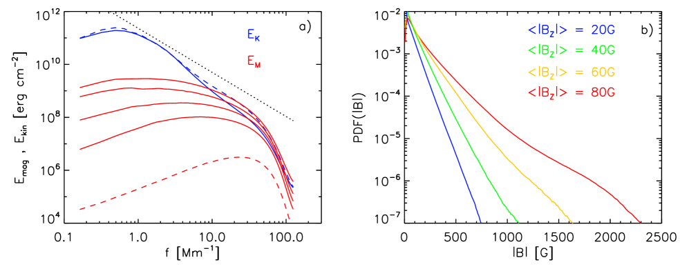
Figure 2.— a) Photospheric ($\tau=1$) power spectra for magnetic energy (red) and kinetic energy (blue) in simulation O4a. The dashed lines correspond to the kinematic growth phase during times when Lorentz-force feedback was negligible. We scaled up the magnetic energy spectrum in order to show clearly in the same figure. The solid red lines correspond bottom to top to snapshots with $20,40,60$, and $80$ G vertical mean field strength at $\tau=1$. For increasing field strength the peak of magnetic power moves toward larger scales. The solid blue line shows the kinetic energy spectrum for the $80$ G case. The dotted line in panel a) indicates a Kolmogorov slope of $-5/3$. b) Probability distribution functions for $|B|$ at $\tau=1$ for vertical mean field strength from $20$ to $80$ G.

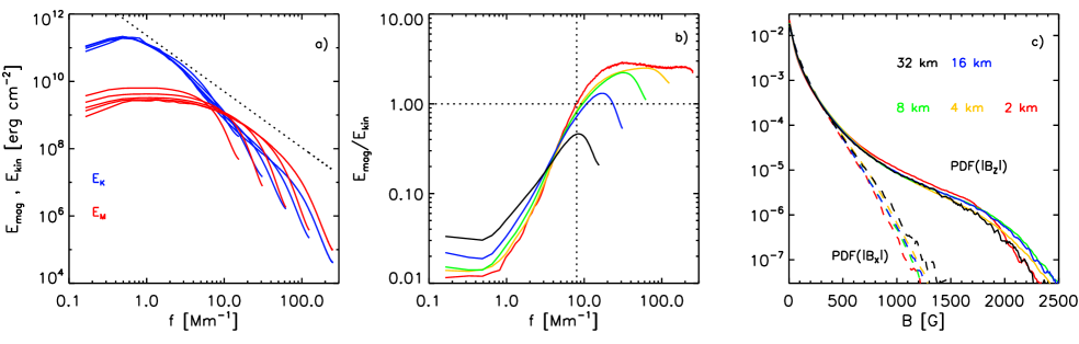
Figure 3.— a) Resolution dependence of magnetic (red) and kinetic (blue) energy power spectra comparing the simulations O32a-O2a. All simulations reached about $80$ G vertical mean field strength at $\tau=1$, the grid spacing was varied from $32$ to $2$ km. The dotted line in panel a) indicates a Kolmogorov slope of $-5/3$. b) Ratio of magnetic to kinetic energy as function of resolution. For grid spacings smaller than $16$ km the magnetic energy is in super-equipartition on scales smaller than about $100$ km. For the highest resolution cases ($4$ and $2$ km) we see some indication that the ratio might reach asymptotically a value around $2$. c) Resolution dependence of the probability distribution function for $|B_{x}|$ and $|B_{z}|$.

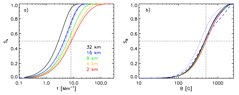
Figure 4.— a) Normalized integrated magnetic energy spectra from Figure 3. For the highest resolution case (grid spacing of $2$ km) $50\%$ of the magnetic energy found at the $\tau=1$ surface is present on scales smaller than $100$ km. b) Normalized integrated magnetic energy distribution functions. $50\%$ of the magnetic energy on the $\tau=1$ surface is found in field with less than $500$ G strength. Solid lines correspond to simulations O32a-O2a with $\langle|B_{z}|\rangle=80$ G, dashed (dotted) lines correspond to simulations O16b and O16bM with $\langle|B_{z}|\rangle=60$ G.

3.1. Kinematic to saturated phase

We start our discussion of results with numerical simulations using the $6.144\times 6.144\times 3.072\,\mbox{Mm}^{3}$ domain and the boundary condition OSa. We limit the horizontal RMS field strength in inflow regions to $600$ G, which corresponds approximately to a solution in which the RMS field strength increases with depth as the same rate as the equipartition field strength. As we will discuss in Section 3.6, these solutions are close to an upper limit for the quiet Sun field strength. We use the small domain to explore the resolution dependence of the results and repeated the same experiment with grid spacings of $32$, $16$, $8$, and $4$ km. All simulations were started from a thermally relaxed $B=0$ G convection simulation to which we added a $10^{-3}$ G seed field (pointing in the z-direction, random in the horizontal plane and uniform in the vertical direction). In addition we present a simulation with $2$ km grid spacing, which was restarted from the $4$ km case.

Figure 1 presents for the simulation with $4$ km grid spacing (O4a) two snapshots, one during the early growth phase (panels a-c) at a time when $\langle|B_{z}|\rangle(\tau=1)=8.4$ G and one during during a later phase (panels d-f) when $\langle|B_{z}|\rangle(\tau=1)=86$ G. The panels a) and d) show the intensity for a vertical ray, panels b) and e) the vertical velocity at $\tau=1$, and the panels c) and f) the vertical magnetic field at $\tau=1$. While the snapshot with $\langle|B_{z}|\rangle(\tau=1)=8.4$ G shows magnetic field organized on scales close to the grid spacing of the simulation, the snapshot with $\langle|B_{z}|\rangle(\tau=1)=86$ G shows magnetic field organized more on the scale of granular downflows with a mostly sheet-like appearance. Several downflow lanes show sheets with opposite polarity nearby. Panel d) shows also several brightness enhancements associated with strong field on scales of $100$ km and less. We provide also 2 animations of Figure 1 in the online material (one for the kinematic and one for the saturated phase). These animation show the same quantities as presented in Figure 1.

Figure 2a) shows kinetic and magnetic energy spectra (at $\tau=1$), which were computed for the $4$ km grid spacing case. As the solution is evolving from the kinematic growth phase to the saturated regime, the peak of the magnetic energy spectrum is moving toward larger scales. At the same time kinetic energy becomes suppressed by about a factor of $2$ on scales smaller than $100$ km as a consequence of Lorentz-force feedback. We will discuss the saturation process further in Section 3.9. For the solution reaching a vertical mean field strength of $80$ G in the photosphere, the magnetic energy is in super-equipartition by about a factor of $2$ on scales smaller than $100$ km.

For the case with $4$ km grid spacing presented here the e-folding time scale for magnetic energy in the photosphere is about $50$ sec during the kinematic growth phase. The growth rate is strongly resolution dependent, we find time scales of $120$, $350$, and $850$ sec for grid spacings of $8$, $16$, and $32$ km. This leads on average to a resolution dependence of the kinematic growth rate $\gamma_{K}\sim\Delta x^{-1.36}$. This resolution dependence is significantly steeper compared to simple estimates that yield for $P_{M}\ll 1$ $\gamma_{K}\sim Re_{M}^{1/2}$, where $Re_{M}=vL/\eta$, $v$ and $L$ are typical velocity and length scales of the problem (for $P_{M}\gg 1$ $Re_{M}$ has to be replaced by $Re=vL/\nu$) . Since we do not have explicit viscosity and magnetic diffusivity we further assume that $Re_{M}$ is linked to the scale separation allowed for by the numerical simulation. Assuming a 5/3 Kolmogorov spectrum, we would expect $Re_{M}\sim\Delta x^{-4/3}$, leading to $\gamma_{K}\sim\Delta x^{-2/3}$. The growth rate is more consistent with a $\gamma_{K}\sim Re_{M}$ dependence, which was also found by Pietarila Graham et al. (2010). Since we do not use here any explicit numerical diffusivity a detailed interpretation is difficult.

Figure 2b) shows the corresponding probability distribution functions (PDFs) for $|B|$ at $\tau=1$. The PDF has a peak at around $30$ G and a nearly exponential drop for stronger field. For the snapshots with $\langle|B_{z}|\rangle>60$ G strong kG field concentrations cause a bulge for $|B|>1000$ G. In snapshots with $\langle|B_{z}|\rangle=80$ G we find at $\tau=1$ field concentrations with more than $2$ kG.

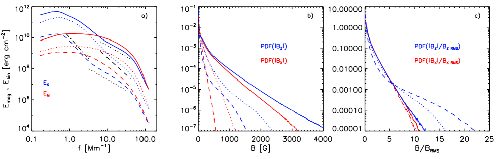
Figure 5.— Comparison of a) power spectra and b), c) probability distribution functions for $|B_{x}|$ and $|B_{z}|$ for 3 different height levels in simulation O4a. Solid lines show quantities in $1$ Mm depth, dotted lines on the $\tau=1$ and dashed lines on the $\tau=0.01$ levels. Panel c) compares normalized PDFs, which allow for a direct comparison of the shape regardless of field strength. In panel a) the black dotted, dashed and dashed-dotted lines indicate $-1.4$, $-2.2$ and $-2.7$ power law slopes, respectively.

3.2. Resolution dependence

Figure 3 compares simulations with 5 different grid spacings ranging from $32$ to $2$ km. The simulation with $2$ km grid spacing was restarted from the saturated $4$ km simulation and evolved for an additional $5$ minutes. Power spectra and PDFs were averaged over snapshots with values of $\langle|B_{z}|\rangle(\tau=1)$ between $75$ and $85$ G. Panel a) shows kinetic (blue) and magnetic (red) energy spectra for the simulations O32a-O2a. Increasing the resolution leads to a convergence of the power spectra on the large scales while smaller scales are added. The simulations with $32$ and $16$ km grid spacing show excess power on large scales, since the same amount of magnetic energy is distributed over less wave numbers. The simulations with $8$ to $2$ km grid spacing do not show a significant difference indicating that a grid spacing of $8$ km or smaller is required to properly represent the energy distribution on larger scales in the photosphere. The dotted line in panel a) indicates a Kolmogorov slope of $-5/3$ as a rough reference. Over the scale-range explored we don’t see a clear indication of a power law for the magnetic energy, there is some indication of power laws for the kinetic energy (see also Figure 5). Panel b) shows the ratio of magnetic to kinetic energy as function of scale. For grid spacings smaller than $16$ km we find a super-equipartition regime on scales smaller than $100$ km and see some indication that the ratio of magnetic to kinetic energy asymptotically reaches a factor of about $2-2.5$. Panel c) shows the PDF for $|B_{x}|$ and $|B_{z}|$ at $\tau=1$. We do not see a systematic dependence on resolution, differences for stronger field are mostly realization noise. For field with less than $500$ G strength the PDFs for $|B_{x}|$ and $|B_{z}|$ are essentially identical. Note that we show here the PDFs for the absolute values of the field components since the simulations do not have any net magnetic flux, leading to symmetric PDFs with respect to $B=0$.

Figure 4 shows normalized integrated magnetic energy spectra and distribution functions for the simulations O32a-O2a (solid lines) . The quantities shown are defined as

$$S_{k} = \frac{\int_{0}^{k}E_{M}(k)dk}{\int_{0}^{k_{max}}E_{M}(k)dk}$$ (19)

$$S_{B} = \frac{\int_{0}^{B}PDF(B)B^{2}dB}{\int_{0}^{B_{max}}PDF(B)B^{2}dB}$$ (20)

The quantity $S_{k}$ shows resolution dependence as expected from Figure 3a). In the highest resolution case about $50\%$ of the magnetic energy in the photosphere on the $\tau=1$ level is found on scales smaller than about $100$ km. Properly resolving the spectral magnetic energy distribution in the photosphere requires grid spacings of $8$ km or smaller. In contrast to this the quantity $S_{B}$ shows only little resolution dependence. In all cases $50\%$ of the magnetic energy is found in regions with $|B|$ of less than $500$ G. Kilo-Gauss field contributes about $10\%$ to the total magnetic energy. For comparison we also show these quantities for the simulation O16b (dotted) and O16bM (dashed). Both simulations have $25\%$ less unsigned flux in the photosphere. The differences in $S_{k}$ are very minor. $S_{B}$ is shifted for the simulation O16b to the left toward weaker field. In contrast to that the simulation O16bM (larger domain) is very similar to the $80$ G cases and has an even larger contribution from kG field. We will discuss kG field concentrations further in Section 3.4.

Figure 6.— Results from run O2a with a grid spacing of $2$ km. a) Intensity, b) $B_{z}(\tau=1)$, c) Intensity patterns magnified for lower left corner of domain. Contour lines indicate regions with $|B|>1$ kG, d) $B_{z}(\tau=1)$ magnified for lower left corner.

3.3. Height dependence

Figure 5 presents how power spectra and probability distribution functions for the magnetic field strength depend on the vertical position in the simulation domain (based on run O4a). Here we focus on three levels that are indicated by different line styles (solid: $-1$ Mm depth, dotted: $\tau=1$, dashed: $\tau=0.01$). Panel a) presents the kinetic and magnetic energy spectra for the three levels. They show the same overall behavior with a super-equipartition regime toward small scales. While the super-equipartition regime is reached at $\tau=1$ for scales smaller than $100$ km, it extends to $500$ km at $\tau=0.01$ since the kinetic energy drops more rapidly than magnetic energy above the photosphere (short density scale height). The super-equipartition regime extends also to moderately larger scales beneath the photosphere, since the overall scale of convective motions increases with the increasing scale height, although the difference is small between $\tau=1$ and $1$ Mm deeper. The black dotted, dashed and dashed-dotted lines indicate power law slopes of $-1.4$, $-2.2$ and $-2.7$, respectively. While we do not find a clear power law for $E_{M}$ at any height level there is some indication of a power law for $E_{k}$ on scales smaller than downflow lanes (few $100$ km). At $1$ Mm depth and $\tau=0.01$ we find slopes of about $-1.4$, while the $\tau=1$ level is with $-2.2$ substantially steeper. Extrapolating the approximate slopes to smaller scales implies that the spectra of $E_{k}$ on the $\tau=1$ and $\tau=0.01$ levels will cross unless there is a change of slope toward smaller scales in either layer, which is more likely. For all three layers we also find steeper slopes on scales larger than a few $100$ km. At $\tau=0.01$ we find with $-2.7$ the steepest slope.

Comparing the PDFs for $|B_{x}|$ and $|B_{z}|$ (panel b) shows systematic differences in the overall shape between the distribution for vertical field at $\tau=1$ and $\tau=0.01$ and the rest. This difference is most obvious if we consider PDFs for the normalized magnetic field components (panel c). Here the PDFs for $|B_{x}|$ at all three height levels and the PDF for $|B_{z}|$ in $1$ Mm depth are essentially identical, while the PDFs for $|B_{z}|$ at $\tau=1$ and $\tau=0.01$ show a much more extended tail toward stronger field. This is a strong indication for the presence of a distinct amplification process operating only on vertical field in the photosphere, while the distribution of $B_{x}$ in all three levels and $B_{z}$ beneath the photosphere is of mostly turbulent origin. While it is non-trivial to separate out the additional amplification process in the photosphere, we conjecture that it is related to a process along the lines of ”convective intensification” (Schüssler, 1990), which is a combination of flux-expulsion, back-reaction of magnetic field leading to partial evacuation, enhanced radiative cooling and related downflows. These processes go beyond the idealized picture of ”convective collapse” (Spruit, 1979).

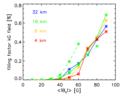
Figure 7.— Filling factor of kG field at $\tau=1$. Solid lines are computed from simulations O32a-O4a, the dotted (dashed) lines corresponds to O16b (O16bM). Field concentrations with more than $1$ kG strength appear independent of resolution once $\langle|B_{z}|\rangle$ exceeds about $30-40$ G. For $80$ G the filling factor reaches about $0.45\%$. This fraction is not systematically dependent on resolution, but does increase with domain size (dashed line).

Figure 8.— a) Intensity and b) $B_{z}$ at $\tau=1$ taken from the simulation O16bM. The lower left corner ($x,y<6.144$ Mm) shows $I$ and $B_{z}$ from the simulation O16b for comparison. The larger domain shows indications of a network structure significantly larger than granulation that cannot form in the small domain. An animation of this figure displaying only O16bM is provided with the online material.

3.4. kG flux concentrations

Figure 1 shows the presence of several kG field concentrations in the photosphere that lead to brightness enhancements in the downflow lanes. Here we analyze in more detail how these flux concentrations depend on the overall field strength as well as domain size.

Figure 6 shows examples of kG flux concentrations in the highest resolution simulation O2a. The panels a) and b) show $I$ and $B_{z}(\tau=1)$ for the full horizontal domain extent, while panels c) and d) show a magnification of the lower left corner of the domain. In panel c) contour lines highlight regions with $|B|>1$ kG. Many kG field concentrations exist on scales smaller than $100$ km down to scales comparable to the grid resolution. Strong magnetic field is typically organized in sheets, often with alternating polarities. kG flux concentrations are small knots along these sheets in which the field strength is increased temporarily due to dynamical effects. Some longer lived flux concentrations may be found in granular downflow vertices. We do not present here a detailed analysis of the temporal evolution of kG field concentrations, but refer the interested reader to the animations of Figure 1 provided with the online material.

Figure 7 presents how the filling factor of kG field at $\tau=1$ depends on the vertical mean field strength, resolution as well as domain depth. To this end we computed for the simulations O32a-O4a the filling factor of regions with $|B|>1$ kG at $\tau=1$, while these simulations were evolving from the kinematic phase into the saturated phase. The data points presented in Figure 7 result from binning snapshots in $\pm 5$ G intervals. For all 4 simulations we find regardless of the resolution that kG flux concentrations appear when the vertical mean field strength exceeds about $30-40$ G at $\tau=1$. For $\langle|B_{z}|\rangle=80$ G around $0.45\%$ of the area is occupied by kG flux concentrations. While the results show some scatter due to realization noise in the simulation domain with small horizontal extent, there is no indication of a systematic resolution dependence of this result.

For comparison we also show the simulations O16b (dotted green) and O16bM (dashed green). While O16b is comparable to O16a, for the same field strength O16bM shows about twice the filling factor. This difference is related to the formation of a larger scale magnetic network structure we discuss further in Section 3.5.

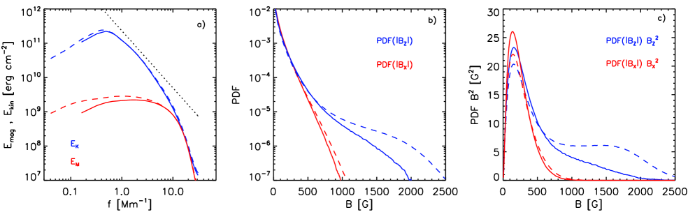
Figure 9.— a) Photospheric ($\tau=1$) power spectra for magnetic energy (red) and kinetic energy (blue) in simulations O16b and O16bM (same resolution, but different domain size). Solid (dashed) lines refer to OS16b (OS16bM). b) Probability distribution functions for $|B_{x}|$ and $|B_{z}|$at $\tau=1$. Increasing the domain size increases the magnetic power at larger scales and leads to a significantly higher fraction of field with more than $1$ kG field strength. c) Distribution of magnetic energy. In the larger domain the quantity $PDF(|B_{z}|)\,B_{z}^{2}$ shows a plateau toward $1700$ G.

3.5. From granular to meso-granular scales

Figure 8 presents a comparison of snapshots from simulations O16b and O16bM. Both simulations have a grid spacing of $16$ km and differ only in domain size. Presented are intensity and the $\tau=1$ magnetograms. In the larger domain magnetic field becomes organized on a scale larger then granulation. We find more pronounced kG flux concentrations that show up mostly as bright features in the intensity image. We do not find the spontaneous formation of larger pore-like field concentrations in O16bM. We provide also an animation of Figure 8 in the online material. The animation shows only the simulation O16bM, but otherwise the same quantities as presented in Figure 8. Figure 9 compares the magnetic and kinetic energy spectra as well as probability distribution function for the simulations O16b and O16bM. We compare here time averages of snapshots with values of $\langle|B_{z}|\rangle$ from $55$ to $65$ G. In the larger domain the magnetic power spectrum extends toward larger scales, while the kinetic energy spectrum continues to fall off. We see an increase of magnetic power on scales larger than about $300$ km, while there is no significant change on smaller scales.

The PDF for $|B_{x}|$ remains mostly unchanged, while the PDF for $|B_{z}|$ shows a significant increase toward kG fields in O16bM. We find that the filling factor of kG field is in O16bM with $0.4\%$ more than twice as large as in O16b ($0.16\%$). Computing the the distribution of energy from vertical magnetic field, $PDF(|B_{z}|)\,B_{z}^{2}$, leads to a plateau toward $1700$ G in O16bM that is not present in the smaller domain. We find the plateau only in the contribution from $B_{z}$. In terms of the fraction of the total magnetic energy that is present in kG field at $\tau=1$ we find the values $9\%$ (O16b) and $23\%$ (O16bM). In addition we studied also similar setups in larger domain ($98.304\times 98.304\times 18.432\,\mbox{Mm}^{3}$) at lower resolution and found that the trends indicated here (mostly flat magnetic energy spectrum on scales larger than granulation, increasing fraction of kG field) continue. In the simulation O32bSG we find a filling factor of $1.1\%$ for kG field, which contribute around $50\%$ to the magnetic energy at $\tau=1$.

The differences we see between the small and large domain arise from the presence of longer-lived, larger-scale convection flows present in the larger domain, which lead to the formation longer-lived flux concentrations. The trend of an increasing fraction of kG field with domain size indicates that perhaps even a super-granular network structure could be maintained by a small-scale dynamo, provided the domain is large enough. While the fraction of kG field increases with domain size, we did not find any indication for a secondary peak in the probability distribution functions of the magnetic field (including O32bSG).

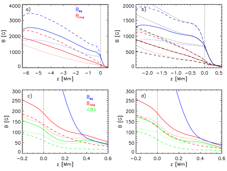
Figure 10.— Comparison of simulations in domains of different depth and horizontal extent. Both simulations use the boundary OSb and have a grid spacing of $16$ km (simulations O16b and O16bM). Panels a) and b) show $B_{\rm eq}$ and $B_{\rm RMS}$ as function of depth. Solid lines correspond to horizontal averages, while dotted (dashed) lines are averages over up- (down-) flow regions. Panel a) shows results for the simulation O16bM ($\sim 6.2$ Mm deep domain), panel b) the same quantities for simulation O16b ($\sim 2.3$ Mm deep domain). Both simulations are consistent with each other in terms of the RMS field strength. Black (dotted) dashed lines indicate in panel b) the profiles of $B_{\rm eq}$ and $B_{\rm RMS}$ from panel a) for comparison. Panels c) and d) show the magnetic field structure at and above the photosphere. Red (green) lines indicate the RMS (mean) field strengths, while blue lines show the equipartition field strength. The meaning of line styles is different from panels a) and b): dashed (dotted) lines refer to the corresponding averages of vertical (horizontal) field components.

3.6. Subsurface field structure, role of boundary conditions

Figure 10 presents for the simulations O16b and O16bM the vertical profiles of the equipartition field strength $B_{\rm eq}$ (blue) and $B_{\rm RMS}$ (red). The equipartition field strength $B_{\rm eq}=\sqrt{4\pi\varrho}\,v_{\rm RMS}$ is a measure for energy available in convective motions. Different line styles correspond to upflow regions (dotted), downflow regions (dashed) and the averages over the whole domain (solid). In Panel b) black lines indicate the profiles from Panel a) for better comparison ($B_{\rm RMS}$ is dashed, $B_{\rm eq}$ dotted). The simulations O16b and O16bM show a lot of similarity, in terms of the total $B_{\rm RMS}$ both simulations match each other in the part of the domain where they overlap. Differences are present when we compare $B_{\rm RMS}$ in up and downflow regions in separation. Also $B_{\rm eq}$ is lower throughout most of the shallow domain, except for the near photospheric layers. The fact that the average magnetic properties in the shallow domain stay very close to those in the deep domain is an indication that the bottom boundary condition OSb does perform fairly well in ”mimicking” a deep convection zone and leads to consistent results independent from the location of the bottom boundary. The panels c) and d) give a more detailed view of the magnetic field structure in and above the photosphere. For both simulations we find a secondary peak of the horizontal mean field strength about $450$ km above $\tau=1$ (green dotted line). In the larger domain, panel c), this translates into a secondary peak of the total field strength, while the RMS field strength continues to drop monotonically above the photosphere. We discuss the inclination of magnetic field above the photosphere in more detail in Figure 14.

Figure 11 presents a comparison of simulations with different bottom boundary conditions. Panel a) compares the boundaries OSb and OZ in the deep (runs O16bM and Z16M) and shallow domain (runs O16b and Z16). Changing from OSb to OZ drops the field strength in the bulk of the convection zone by about a factor of $2$. The difference between both boundary conditions does not depend on the domain depth within the range explored here. The boundary condition OZ is very conservative in the sense that it assumes that the deeper convection zone is field free, which is unlikely to be the case. But even with this assumption a still considerable amount of magnetic field is maintained within the computational domain, although the mean vertical magnetic field at $\tau=1$ levels out at about $30$ G. This value is not strongly dependent on resolution as long as a critical value is passed (i.e. the kinematic dynamo growth rate has to be sufficiently large compared to the flux loss rate $\sim v_{z{\rm RMS}}/H_{\varrho}$). We repeated this experiment with the resolutions from $32$ to $8$km. While we find for $32$ km resolution only a vertical magnetic field strength of $20$ G at $\tau=1$, the simulations with $16$ and $8$ km grid spacing reach both values around $30$ G.

The simulations with the boundary condition OSb reach $>0.5B_{\rm eq}$ in the deeper parts of the domain. These solutions are not far from an upper bound for the field strength in which $B_{\rm RMS}$ and $B_{\rm eq}$ increase with depth at the same rate. To better illustrate this asymptotic limit we show also the results from O32bSG, which uses a $18$ Mm deep domain. The dotted lines indicate $B_{\rm RMS}$ profiles for O16bM and O32bSG that are rescaled by a factor of $1.5$ to illustrate this asymptotic limit. Substantially stronger field would require a $B_{\rm RMS}$ increasing with depth faster than $B_{\rm eq}$ and exceeding equipartition in only a few Mm of depth. This asymptotic limit corresponds to a solution with $\langle|B_{z}|\rangle=85$ G, $\langle B\rangle=160$ G, and $B_{\rm RMS}=275$ G at $\tau=1$.

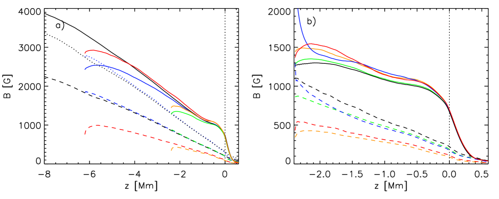
Figure 11.— Comparison of different bottom boundary conditions for a fixed grid spacing of $16$ km. Solid (dashed) lines correspond to equipartition (RMS) field strength, the color indicates simulations with different bottom boundary conditions. In panel a) we compare boundary OSb: O16bM (blue) and O16b (green) with boundary OZ: Z16M (red) and Z16 (orange). The black line show the results from O32bSG, for which the bottom boundary is in about $18$ Mm depth. In addition the dotted lines show scaled subsurface $B_{\rm RMS}$ profiles for O16bM and O32bSG to indicate a solution we consider the upper limit ($B_{\rm RMS}$ increases with depth at the same rate as $B_{\rm eq}$). This solution corresponds to about $\langle|B_{z}|\rangle=85$ G at $\tau=1$ (based on O16bM). Panel b) presents additional experiments in the shallow domain. Here we present simulations with the boundaries OSa (O16a, black), OSb (O16b, green), OZ (Z16, orange), OV (V16, red) and CH (C16, blue).

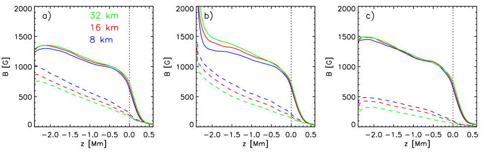
Figure 12.— Resolution dependence of $B_{\rm RMS}$ (dashed) and $B_{\rm eq}$ (solid) for simulations with the boundary a): OSb, runs O32b-O8b; b) CH, runs C32-C8; and c) OZ, runs Z32-Z8.

Figure 11b) compares results of all 5 boundary conditions considered here for the shallow domain. We do not find a significant difference between zero field in inflows OZ (orange) and vertical field everywhere at the bottom boundary OV (red). Due to the strong horizontal divergence in upflows, vertical magnetic field present at the bottom boundary condition becomes quickly expelled from upflows. Solutions with stronger magnetic field require the presence of horizontal field in upflow regions, which is less affected by horizontally divergent flows. The solutions with the boundary conditions OSa,b (black, green) are very similar to a solution computed with a closed bottom boundary condition CH (blue). The saturation field strength for the latter is fully determined by processes within the computational domain, while the former exchange magnetic field through the bottom boundary.

Figure 12 analyses further the resolution dependence of the saturation field strength for the simulations using the boundaries OSb, CH, and OZ. In all three cases we find a similar trend of increasing $B_{\rm RMS}$ with resolution. While the saturation field strength is not yet fully converged, it cannot grow much further in the simulations with the boundary conditions OSb and CH without creating a super-equipartition regime near the bottom of the domain.

3.7. Subsurface Poynting flux and energy conversion rates

Figure 13a) shows the Poynting flux for the simulations O16bM and Z16bM. The flux is normalized by the solar photospheric energy flux of $F_{\odot}=6.3\cdot 10^{10}\,\mbox{erg}\,\mbox{cm}^{-2}\,\mbox{s}^{-1}$. Although we have magnetic energy entering the domain in upflow regions in simulation O16bM (solid lines) using the boundary condition OSb, the magnetic energy leaving the domain in downflow regions over-compensates this contribution by more than a factor of $6$. In the simulation Z16M (dashed lines) the Poynting flux is zero in upflow regions at the bottom boundary by construction (boundary condition OZ). However, about $1-2$ Mm above the bottom boundary mixing between up and downflows provided enough field in upflow regions to have also here an upward directed Poynting flux. The relative contributions from up and downflows in case Z16M are almost identical with case O16bM if we stay $1-2$ Mm away from the bottom boundary condition. Panel b) shows the resulting magnetic energy loss rates for both simulations, which are defined as (with the Poynting flux $P(z)$)

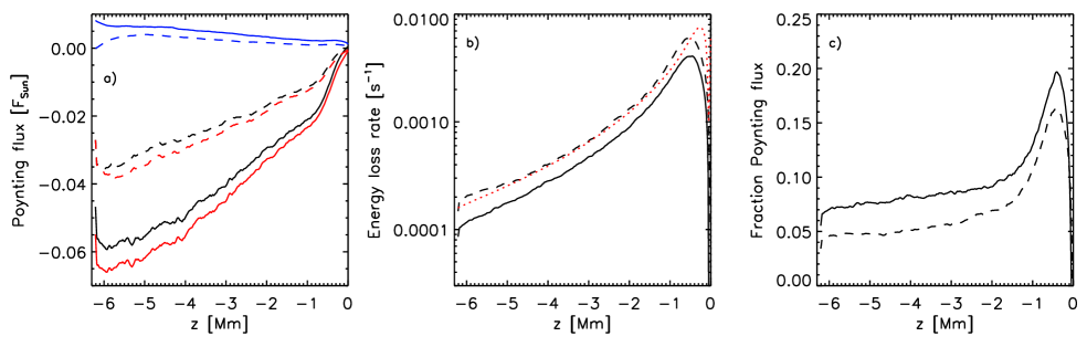
Figure 13.— Comparison of Poynting flux and associated time scales for the simulations O16bM (solid) and Z16M (dashed). a) Black lines show the horizontally averaged Poynting flux, blue and red lines present the contributions from up and downflows. b) Energy loss rate due to Poynting flux ($\zeta(z)$, Eq. 21). The red dotted line indicates a convective overturning time scale $v_{z{\rm RMS}}/H_{\varrho}$. c) Fraction of energy transported by Poynting flux relative to energy converted by Lorentz force ($\varepsilon(z)$, Eq. 22).

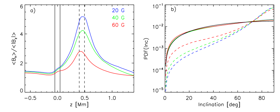
Figure 14.— a) Ratio of horizontal to vertical field strength as function of height. Different colors refer to simulations with the average vertical field strength at $\tau=1$ as indicated. The ratio of horizontal to vertical field has a maximum about $450$ km above $\tau=1$ and is strongly dependent on the overall field strength of the simulation and decreases with increasing field strength. b) Probability distribution functions for the field inclination with respect to the vertical. Solid lines refer to the deep photosphere around $\tau=1$, dashed lines to about $450$ km height as indicated in panel a). The black solid line indicates an isotropic distribution of field inclinations.

$$\zeta(z)=\frac{-P(z)}{\int_{z}^{z_{top}}E_{M}\,{\rm d}z}\;,$$ (21)

i.e. we compare the Poynting flux at a height $z$ to the total magnetic energy of the domain above $z$. For this analysis we can ignore the Poynting flux at the top boundary, which is around $10^{-5}F_{\odot}$. In simulation Z16M with zero magnetic field in inflow regions we find an about $1.8$ times larger loss rate. The vertical profile of $\zeta$ agrees very well with a convective time scale $v_{z{\rm RMS}}/H_{\varrho}$, indicated by a red dotted line. The kinematic growth phase of the dynamo is not affected by details of the bottom boundary condition as long as the growth rate fullfils $\gamma_{K}\gg v_{z{\rm RMS}}/H_{\varrho}$ (this condition is fulfilled well by the higher resolution cases with a grid spacing of $8$ km or smaller, for the cases with $16$ and $32$ km grid spacing this condition is fulfilled in the lower parts of the domain, but not in the photosphere). The bottom boundary matters when non-linear saturation effects cause $\gamma(B)\rightarrow v_{z{\rm RMS}}/H_{\varrho}$. The simulation Z16M presents a setup with the maximum possible energy loss at the bottom boundary, since the time-scale of magnetic energy loss is the same as the time scale for mass exchange. In that sense this setup presents a lower limit for an efficient dynamo with $\gamma_{K}\gg v_{z{\rm RMS}}/H_{\varrho}$ (a less efficient dynamo could have of course an even lower saturation field strength). Stronger saturation field strengths require less leaky bottom boundary conditions, which require the presence of a Poynting flux in upflow regions, like in O16bM.

Panel c) compares the energy lost by the Poynting flux to the energy converted via the Lorentz force in the domain above a height $z$:

$$\varepsilon(z)=\frac{P(z)}{\int_{z}^{z_{top}}\mathbf{v}\cdot(\mathbf{j}\times\mathbf{B})\,{\rm d}z}\;.$$ (22)

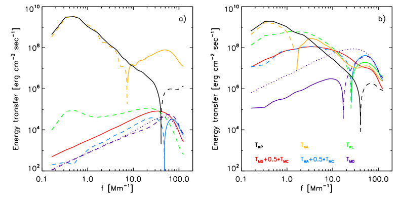
Figure 15.— Energy transfer functions for the simulation O16a with $4$ km grid spacing. Panel a) shows the kinematic growth phase, panel b) the saturated phase. The line color corresponds to contributions from pressure/buoyancy (black), advection of momentum (yellow), Lorentz force (green), stretching of magnetic field (red), and advection of magnetic field (blue). Contributions from the magnetic compression term are split 50/50 among stretching and advection. Solid lines correspond to positive contributions, dashed lines to negative contributions. Contributions from numerical diffusivity in the induction equation are indicated by the purple lines. Here the dotted line shows a Laplacian diffusivity with $\eta=5\cdot 10^{9}\,\mbox{cm}^{2}\mbox{s}^{-1}$ for comparison.

This fraction is lower in Z16M because of non-linear saturation effects in O16bM, which affect $\mathbf{v}\cdot(\mathbf{j}\times\mathbf{B})$ more strongly than $(\mathbf{v}\times\mathbf{B})\times\mathbf{B}$ (see also Figure 16). While the simulation domain of O16bM contains almost $4$ times the magnetic energy of Z16M, the average amount of energy converted from kinetic to magnetic energy is in both simulations comparable within a few $\%$, i.e. $85\,\mbox{erg}\,\mbox{cm}^{-3}\,\mbox{s}^{-1}$ (O16bM) and $80\,\mbox{erg}\,\mbox{cm}^{-3}\,\mbox{s}^{-1}$ (Z16M), which is about $50\%$ of the energy conversion by pressure/buoyancy forces in the domain, see also Section 3.9 for further detail. Integrated over the depth of the domain this energy conversion rate equals to about $80\%$ of the energy flux through the domain. Note that we discuss here conversion rates between energy reservoirs and not true sinks of energy, since the energy is returned to internal energy through dissipation processes. The conversion rates can be comparable or even exceed the energy flux through the system. Most of the energy converted from kinetic to magnetic is preferentially dissipated in downflow regions, while work against the Lorentz force reduces the kinetic energy there. This changes the overall balance of convective energy transport by reducing the contribution from the kinetic energy flux. We find in a non-magnetic convection simulation in $6$ Mm depth a downward directed kinetic energy flux of about $-0.3\,F_{\odot}$, this value is reduced to $-0.2\,F_{\odot}$ in simulation O16bM.

Recently Hotta et al. (2014) presented small-scale dynamo simulations in a global setup covering the convection zone up to $7$ Mm beneath the photosphere. Using a similar numerical approach, but a substantially lower grid spacing of $1100$ km horizontally and $375$ km vertically, they were able to maintain a field with $0.15-0.25\,B_{\rm eq}$ throughout the convection zone. The maintenance of the field requires in their setup around $5-10\,\mbox{erg}\,\mbox{cm}^{-3}\,\mbox{s}^{-1}$, which is consistent with our results considering the differences in the overall field strength reached (their field near the top boundary falls short of our values by a factor of $4$, which is reflected in a more than a factor of $10$ lower energy conversion rate). Integrated over the entire convection zone the energy conversion rate by a small-scale dynamo could account to as much as few $L_{\odot}$ ($L_{\odot}=3.84\cdot 10^{33}\mbox{erg}\,\mbox{s}^{-1}$). Compared to that the energy extracted from large-scale mean flows in mean field dynamo models (Rempel, 2006) as well as 3D global dynamo simulations (Nelson et al., 2013) is about 2 orders of magnitude smaller.

3.8. Horizontal magnetic field above $\tau=1$

In Figure 14 we further analyze how the ratio of horizontal and vertical field as well as distribution of inclination angles varies as function of height. In Panel a) we present the quantity $\langle(B_{x}^{2}+B_{y}^{2})^{0.5}\rangle/\langle|B_{z}|\rangle$ as function of height for the simulation O16bM. Since this simulation was started from a weak seed field we selected during the growth phase 3 snapshots with the field strength of $\langle|B_{z}|\rangle=20$, $40$, and $60$ G at $\tau=1$. We find that independent from the field strength $\langle(B_{x}^{2}+B_{y}^{2})^{0.5}\rangle/\langle|B_{z}|\rangle$ peaks about $450$ km above $\tau=1$. The peak value reached drops monotonically with increasing field strength from about $5$ at $20$ G to $2.75$ at $60$ G. The dashed vertical lines indicate regions for which we computed the PDFs for the inclination angle with respect to the vertical direction (panel b). Solid lines refer to the PDFs around $\tau=1$, while dashed lines correspond to about $450$ km height. For reference the black line indicates the distribution for an isotropic field. For all three field strengths shown the PDFs are close to isotropic in the deep photosphere, but strongly skewed toward horizontal field in $450$ km height. The contribution from horizontal field is strong enough to create a distinct peak in the field strength about $450$ km above $\tau=1$ as presented in Figure 10, panel c).

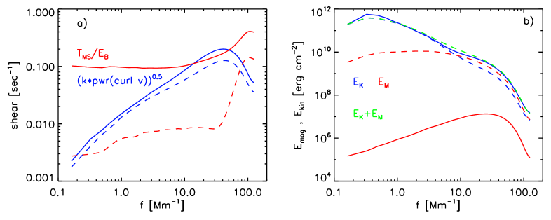
Figure 16.— Saturation of the dynamo comparing the kinematic growth phase with the saturated phase of O4a. Panel a) shows the vorticity spectrum $\sqrt{k\,P(\omega)}$ (blue) and $T_{MS}/E_{M}$ (red). Solid (dashed) lines indicate the kinematic (saturated) phase. Panel b) shows the corresponding kinetic energy and magnetic energy power spectra.

3.9. Transfer functions and saturation process

Figure 15 presents energy transfer functions computed for the simulation O4a (4 km grid spacing). We compare here the kinematic growth phase (panel a) with the saturated phase (panel b). The transfer functions are computed at a depth of about $800$ km beneath the photosphere. They are averaged over a depth range of $160$ km. In addition we conducted a time average and applied smoothing to the transfer functions in order to suppress realization noise. Since the magnetic energy is varying rapidly during the kinematic growth phase we normalized the transfer functions that depend on the magnetic field by the total magnetic energy in each time step and averaged the normalized transfer functions (the kinematic growth is self-similar, i.e. only the amplitude and not the shape of the transfer functions is changing). In Figure 15a) we scaled the corresponding transfer functions arbitrarily to show them on the same scale as the non-magnetic ones.

Colors refer to the transfer function defined in the Appendix. The energy transfers to the kinetic energy reservoir are $T_{KP}$ (black, energy transfer by pressure and buoyancy), $T_{KA}$ (orange, kinetic energy transfer by advection), and $T_{KL}$ (green, kinetic energy transfer by the Lorentz force). The energy transfers to the magnetic energy reservoir are $T_{MS}+0.5\,T_{MC}$ (red, energy transfer by stretching and compression), $T_{MA}+0.5\,T_{MC}$ (blue, energy transfer by advection and compression), and $T_{MD}$ (purple, energy transfer due to magnetic numerical diffusivity). Solid (dashed) lines indicate positive (negative) contributions, the purple dotted lines indicate the transfer of a Laplacian magnetic diffusivity with $\eta=5\cdot 10^{9}\,\mbox{cm}^{2}\mbox{s}^{-1}$ for comparison (the simulations were only run with numerical diffusivity). We do not show the terms $T_{KD}$ for better readability of the figures. We also split the term $T_{MC}$ $50/50$ among $T_{MA}$ and $T_{MS}$. The reason for this (apart from reducing the number of quantities shown in Figure 15) is that we can expand the underlying terms as:

$$-\mathbf{B} \cdot \left((\mathbf{v}\cdot\nabla)\mathbf{B}+\frac{\mathbf{B}}{2}\nabla\cdot\mathbf{v}\right)=-\nabla\cdot\left(\mathbf{v}\frac{B^{2}}{2}\right)$$ (23)

$$\mathbf{B} \cdot \left((\mathbf{B}\cdot\nabla)\mathbf{v}-\frac{\mathbf{B}}{2}\nabla\cdot\mathbf{v}\right)=\nabla\cdot\left(\mathbf{B}(\mathbf{v}\cdot\mathbf{B})-\mathbf{v}\frac{B^{2}}{2}\right)$$ (24)

$$-\mathbf{v}\cdot\nabla\cdot\left(\mathbf{B}\mathbf{B}-\frac{1}{2}\mathbf{I}\,B^{2}\right)$$

i.e. the terms underlying $T_{MA}+0.5T_{MC}$ (Eq. 23) can be identified with an advective energy transport within the magnetic energy reservoir analogous to the terms underlying $T_{KA}$ that refer to the turbulent momentum cascade. The terms underlying $T_{MS}+0.5T_{MC}$ (Eq. 24) describe in part a transport within the magnetic energy reservoir (remaining non-advective terms of Poynting flux) and in part the energy transfer with the kinetic energy reservoir (via Lorentz force).

During the kinematic growth phase (panel a) $T_{MS}+0.5T_{MC}$ peaks on a scale of about $25-30$ km, which is about about $6-8\,\Delta x$, i.e. close to the smallest features that can be resolved with the given grid spacing. With increasing resolution this scale is decreasing as it stays near $6-8\,\Delta x$. The corresponding Lorentz force related energy transfer $T_{KL}$ shows two peaks, one at around $50$ km and one around $2$ Mm. The peak at around $50$ km is related to the magnetic tension force, while the peak at $2$ Mm is caused by magnetic pressure. The dominant contribution to the energy exchange comes from the peak at small scales. On scales larger than $20$ km $T_{MS}+0.5T_{MC}$ is partially opposed by the transport term $T_{MA}+0.5T_{MC}$ and a numerical diffusion term of similar amplitude. The remainder leads to an exponential growth of magnetic energy with a e-folding time scale of about $50$ sec. On scales smaller than $20$ km positive contributions from $T_{MS}+0.5T_{MC}$ and $T_{MA}+0.5T_{MC}$ are opposed by numerical diffusivity. The contribution from numerical magnetic diffusivity (dashed purple line) is on scales larger than $100$ km very similar to a Laplacian diffusivity with $\eta=5\cdot 10^{9}\,\mbox{cm}^{2}\mbox{s}^{-1}$ (dotted purple line), moderate differences exist on smaller scales. However, replacing our numerical diffusivity with Laplacian diffusivity of $\eta=5\cdot 10^{9}\,\mbox{cm}^{2}\mbox{s}^{-1}$ leads to an about $6$ times smaller kinematic growth rate of the dynamo, which implies that it is non-trivial to estimate the effective numerical diffusivity by looking at transfer functions or energy dissipation rates.

In the saturated phase (panel b) $T_{MS}+0.5T_{MC}$ peaks on a scale of about $250-300$ km, about a factor of $10$ larger than during the kinematic growth phase. Similarly $T_{KL}$ peaks now at a scale of $500$ km, i.e. most of the energy transfers from kinetic to magnetic energy happen on a scale comparable to downflow lanes. Unlike the kinematic growth phase these scales are independent of resolution and realized in all simulations presented here regardless of their resolution. On scales larger than $100$ km $T_{MS}+0.5T_{MC}$ is in balance with $T_{MA}+0.5T_{MC}$, contributions from numerical diffusivity, $T_{MD}$, are about 2 orders of magnitude smaller. While $T_{MD}$ was close to Laplacian during the kinematic growth phase, it differs substantially during the saturated phase. Contributions on scales larger than about $70$ km are in amplitude about a factor of $10$ smaller than a Laplacian with $\eta=5\cdot 10^{9}\,\mbox{cm}^{2}\mbox{s}^{-1}$ (dotted purple line) and have the opposite sign. The latter is related to the cutoff we introduced in Eq. (10) for a setting of $h=2$. Integrated over all scales the positive contribution accounts to about $1.7\%$ of the total unsigned dissipation. The sign change is not present for grid spacings of $8$ km and larger and can be avoided by using a setting of $h=1$ in higher resolution cases (with no significant difference to the obtained results). On the smallest scales the contribution from numerical diffusivity remains similar to a Laplacian diffusivity with $\eta=5\cdot 10^{9}\,\mbox{cm}^{2}\mbox{s}^{-1}$.

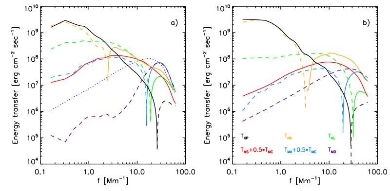
Figure 17.— Energy transfer functions for simulations C8 and C8$\eta$ with $8$ km grid spacing using the boundary CH. The meaning of the line styles is the same as in Figure 15. Panel a) shows a simulation computed with artificial magnetic diffusivity, panel b) a simulation computed with a Laplacian diffusivity using a values of $\eta=10^{10}\,\mbox{cm}^{2}\mbox{s}^{-1}$. The dotted purple line in panel a) indicates a Laplacian diffusivity with $\eta=10^{10}\,\mbox{cm}^{2}\mbox{s}^{-1}$ for comparison.

In the saturated phase the Lorentz force is a dominant contributor in the momentum equation and dominates energy transfers on scales smaller than $500-1000$ km. While we find in the kinematic growth phase a balance between pressure/buoyancy driving, $T_{KP}$, and the kinetic energy cascade, $T_{KA}$, down to scales of about $150$ km, this balance is only realized on scales larger than $1000$ km in the saturated phase. From scales of $500$ km down to scales of $50$ km the term $T_{KA}$ balances mostly $T_{KL}$ and as a consequence the amount of kinetic energy that is transported to small scales by $T_{KA}$ is significantly reduced. Not all of the energy that is extracted by the Lorentz force is transferred into magnetic energy. On scales smaller than $40$ km $T_{KL}$ becomes the dominant source of kinetic energy. Overall $30\%$ of the energy extracted from kinetic energy on large scales is returned to kinetic energy on small scales. Comparing transfer functions computed for simulations with different resolution, we find that this fraction increases with resolution.

The total amount of energy that is dissipated numerically is within $10\%$ the same between kinematic and saturated phase. In the saturated phase about $55\%$ of the energy dissipation happens through the magnetic channel. That we find about the same energy dissipation rates from magnetic and viscous dissipation is possibly related to an intrinsic numerical $P_{M}$ close to $1$. Brandenburg (2011) found that this ratio depends on $P_{M}$ and that more energy is dissipated through the magnetic channel for low $P_{M}$.

Figure 16a) analyzes the saturation mechanism of the dynamo. To this end we compare the vorticity spectrum and the normalized transfer function $T_{MS}/E_{M}$ between kinematic growth phase and saturated phase. We present these quantities averaged over the same depth range as the transfer functions in Figure 15. We see only a moderate reduction of the overall shear by about $40\%$, mostly on smaller scales. $T_{MS}/E_{M}$ drops by more than a factor of $10$, which indicates that most of the saturation happens though a misalignment of magnetic field and velocity shear. Panel b) shows the corresponding kinetic and magnetic energy spectra, which are not very different from the photospheric spectra shown in Figure 2. In the saturated phase kinetic energy is suppressed on scales smaller than $100$ km and magnetic energy is in super equipartition by about a factor of $1.7$. The sum of kinetic and magnetic energy in the saturated phase is similar to the kinetic energy during the kinematic phase.

Figure 17 compares a solution computed with numerical diffusivity (panel a) to a solution computed with a Laplacian magnetic diffusivity using $\eta=10^{10}\,\mbox{cm}^{2}\mbox{s}^{-1}$. These simulations are both computed with a closed bottom boundary, i.e. the saturation level reached is determined by processes within the computational domain and not sensitive to the magnetic bottom boundary condition. We present the same quantities as in Figure 15. In panel a) the dotted purple line shows the transfer functions of a Laplacian diffusivity with the same values as in panel b) for comparison. The solution computed with a Laplacian diffusivity saturates at about half the field strength compared to the case with only numerical diffusivity. The differences seen in the transfer functions for both cases are mostly a reflection of the differences in overall field strength, i.e. we see the peak of $T_{MS}+0.5T_{MC}$ shifted toward smaller scales as expected. The contribution from numerical diffusivity on large scales in panel a) is by about one order of magnitude smaller than the contribution from the Laplacian diffusivity in panel b) (relative to the terms $T_{MS}+0.5T_{MC}$. The value of $\eta=10^{10}\,\mbox{cm}^{2}\mbox{s}^{-1}$ is very close to the smallest value we can use for a grid spacing of $8$ km without excessive ringing and numerical instability on small scales. Achieving a regime similar to that shown in panel a) on large scales using a Laplacian magnetic diffusivity would likely require about 10 times higher resolution, i.e. $10^{4}$ times more computing time.

4. Discussion

Since a significant fraction of the magnetic energy in the presented simulations is found on scales smaller than the resolution of current instrumentation, a detailed comparison with observations is only possible through spectro-polarimetric forward modeling. We defer such in-depth comparison to future publications, and limit the discussion here to a more qualitative level.

4.1. Field strength of quiet Sun

We presented a series of simulations that lead to saturation field strength about a factor of $2-3$ higher than previously found by Vögler & Schüssler (2007). We achieved that by a combination of a sufficiently high resolution in combination with an LES approach (i.e. sufficient low numerical diffusivities) and different bottom boundary conditions. Higher resolution alone is not sufficient, we found that the bottom boundary condition plays a crucial role. Using a conservative boundary assuming zero magnetic field in inflow regions or only vertical magnetic field (similar to Vögler & Schüssler (2007)), we obtain a lower limit of about $\langle|B_{z}|\rangle=30$ G at $\tau=1$. The term ”lower limit” refers here to efficient dynamos, which have a growth rate $\gamma_{K}\gg v_{z{\rm RMS}}/H_{\varrho}$ during their kinematic phase. Less efficient dynamos can have of course a lower saturation field strength. We derive an upper asymptotic limit of about $85$ G based on the assumption that $B_{\rm RMS}$ cannot increase faster with depth than $B_{\rm eq}$. While our lower limit is possibly affected by the overall dynamo efficiency including potential magnetic Prandtl-number effects we do not account for, the upper limit is only set by the available kinetic energy of the near surface convection zone. Similar values are also found in a setup with a closed bottom boundary, which, while less solar-like, provides a better posed dynamo problem. If we take our simulation O16bM as basis for the extrapolation, our ”upper limit” of $\langle|B_{z}|\rangle=85$ G implies a value of $B_{\rm RMS}=275$ G, $\langle B\rangle=160$ G, and $\langle B_{h}\rangle=120$ G (all at $\tau=1$). These values are similar to those found by Danilovic et al. (2010) through spectropolarimetric forward modeling of rescaled dynamo models and comparison with observations ($\langle|B_{z}|\rangle=84$ G, $\langle B\rangle=170$). We have repeated their analysis with non-grey versions of some of the simulations presented here (Danilovic $\&$ Rempel in prep.) and found that a model with $\langle|B_{z}|\rangle=60$ G agrees best with the data used in Danilovic et al. (2010). The difference comes from the fact that due to non-linear feedback a rescaled weak-field solution is not identical to the fully non-linear strong field solutions we consider here. Inversion results by Orozco Suárez & Bellot Rubio (2012) ($\langle|B_{z}|\rangle=64$ G, $\langle B\rangle=220$) lead to similar values for $\langle|B_{z}|\rangle$, but significantly stronger field strength, which is due to an about a factor of $2$ stronger horizontal field ($198$ G) in their case..

Trujillo Bueno et al. (2004) and Shchukina & Trujillo Bueno (2011) inferred from Hanle depolarization measurements values of $\langle B\rangle$ around $130$ G a few $100$ km above $\tau=1$. If we use our upper limit as reference, we find a field strength in that height range around $80-90$ G, about a factor of $1.5$ less. If we use a model with $\langle|B_{z}|\rangle=60$ G (best fit to Hinode Zeeman data) the disagreement is almost a factor of $2$.

Overall these results indicate that the quiet Sun is magnetized near the upper limit we find, i.e. the observed field strength implies that the subphotospheric layers have to be magnetized close to equipartition. The experiments with $B=0$ at the bottom boundary indicate that a small-scale dynamo restricted to the top $1-2$ Mm of the convection zone could only explain about $50\%$ of the observationally inferred field strength, i.e. the origin and strength of the quiet Sun magnetic field cannot be understood in separation from the deeper layers of the convection zone.

4.2. Scales beyond granulation

We presented one simulation on meso-granular scales using a domain $25$ Mm wide and $6$ Mm deep. Compared to the smaller domains in which no scales larger than granulation are allowed for, this simulation shows an organization of magnetic field on scales larger than granulation and also a stronger contribution from kG field. On a fundamental level this shows that the organization of magnetic field on a wide range of scales is not inconsistent with a small-scale dynamo, provided that the small-scale dynamo operates itself on a wide range of scales. The latter is a natural consequence of stratified convection in larger domains and does not require the contribution from a global dynamo, although that contribution becomes unavoidable once the domain size approaches scales on which rotation and shear become important. In that case a separation of contributions from a small-scale and large-scale dynamo is not trivial and not necessarily meaningful.

4.3. Coupling between the large- and small-scale dynamos

In our numerical experiments we focused entirely on setups with no imposed netflux, which leads to the question of how the presence of a (cyclic) mean field produced by a large-scale dynamo might influence these results. We conducted an additional experiment (similar to O16bM) in which we imposed initially a vertical mean field of $30$ G. We found roughly a doubling of the photospheric magnetic energy, which is mostly due to the formation of a strong meso-granular network with $|B|>1$ kG, while the core of the probability distribution functions remains unchanged (the magnetic energy in regions with $|B|<500$ G is unchanged, in regions with $|B|<1$ kG we find only a $10\%$ increase). This result is expected since there is little recirculation of mass in the top layers of the convection zone. The imposed netflux is expelled quickly into longer lived downflow regions forming a magnetic network structure. The resulting inter-network regions are mostly void of netflux and have properties similar to a simulation without any netflux. A similar weak dependence of the strength of inter-network field and the strength of the surrounding network field was also found by Lites (2011) in Hinode data. Overall this indicates that the strength of mixed polarity field in the photosphere is only weakly influenceable by a vertical mean field. A much stronger modulation is possible through the properties of horizontal field in upflows regions, which is reflected in the strong dependence of our results on the details of the bottom boundary condition. How much the strength of the quiet Sun is modulated by such a coupling depends ultimately on how strongly the large-scale mean and small-scale mixed polarity field in the bulk of the convection zone vary throughout the cycle. Current global dynamo models do not have sufficient resolution to properly capture small-scale field and likely underestimate its contribution. As discussed in Section 3.7 our estimates indicate that the energy converted by small-scale induction effects exceeds the induction by large-scale mean flows (mostly differential rotation) by about two orders of magnitude.

There are also possible feedbacks from the small-scale on the large-scale dynamo as well as convective dynamics. The presence of small-scale field suppresses turbulent motions and reduces the kinetic energy flux. The amount of energy taken out of convective motions through the Lorentz-force is substantial, if we equate this energy transfer with a viscous energy transfer we would require an effective viscosity of a few times $10^{11}\mbox{cm}^{2}\mbox{s}^{-1}$ to mimic this effect. Recently Fan & Fang (2014) showed that the presence of magnetic field in the convection zone can be crucial for maintaining a solar-like differential rotation and that the contribution of the magnetic field can be approximated to some degree by an enhanced effective viscosity of the flow. To which degree small- and large-scale field components contribute to this effects requires further investigation.

4.4. Distribution functions, kG field concentrations

We find that probability distribution functions are very robust, i.e. they barely depend on numerical resolution (we varied the grid spacing by a factor of $16$!). The shape of PDFs is mostly determined by the average field strength and domain size. For a given average field strength we find more strong field in a larger domain. Comparing photospheres with $\langle|B_{z}|\rangle=80$ G we find that $50\%$ of the energy comes from field with less than $500$ G, kG field concentrations contribute about $16\%$ to the total energy. The latter drops to $9\%$ for a $60$ G case and increases to $23\%$ for a $60$ G case in a larger domain. In our simulations the filling factor of kG field concentrations is strongly field strength dependent. More than $\langle|B_{z}|\rangle\sim 30-40$ G is required at $\tau=1$ before they form and the filling factor increases steeply as the field strength increases beyond that threshold. Comparing the shape of normalized PDFs for vertical and horizontal field components we find that the PDFs for vertical field in the photosphere deviate substantially from those of horizontal field as well as vertical field beneath the photosphere (see Figure 5). This is a strong hint for the presence of a convective intensification mechanism (Schüssler, 1990) that is restricted to the photosphere and mostly affects vertical field. While we find strong field at $\tau=1$ reaching up $2.5$ kG, this field component is not organized in form of flux tubes, nor does it have a preferred scale around $100$ km. Strong magnetic field is typically organized in sheets, often with alternating polarities. kG flux concentrations are small knots along these sheets in which the field strength is increased temporarily due to dynamical effects. We find kG flux concentrations down to the smallest scales we can resolve. The kG field present in our simulations does not produce a distinct feature in the PDFs like a secondary peak around kG field strength found in many observations (Ishikawa & Tsuneta, 2009; Lites, 2011; Orozco Suárez & Bellot Rubio, 2012). These observation also indicate that the second peak is possibly caused by contributions from network field and may not be present for inter-network field alone.

4.5. Power spectra

In our highest resolution simulation (grid spacing of $2$ km) we find that about $50\%$ of the magnetic energy in the deep photosphere is found on scales smaller than $100$ km. Therefore properly reproducing the spectral energy distribution requires the highest possible resolution. Performing simulations with lower resolution will artificially move magnetic energy toward larger scales in spectral space, for example we find $50\%$ on scales smaller than $300$ km for a grid spacing of $32$ km. On scales smaller than $100$ km magnetic energy is in super-equipartition buy about a factor of $2$. A similar feature has been found in several small-scale dynamo simulations and LES models of MHD turbulence (see, e.g., review by Brandenburg et al., 2012). We further find that the sum of kinetic and magnetic energy power spectrum in the saturated state is similar to the kinetic energy power spectrum of a pure HD simulation, i.e. kinetic energy is suppressed on scales smaller than $100$ km and that gap is filled with magnetic energy. Even in the highest resolution case it is difficult to identify power laws, in particular for magnetic energy. We see some indication for power laws in the kinetic energy. Steeper slopes (as steep as $-2.7$) are typically found for scales larger than a few $100$ km (width of downflow lanes). On smaller scales the slope is height dependent, we find $-1.4$ at $\tau=0.01$ and $1$ Mm beneath $\tau=1$, while we see a steeper $-2.2$ slope at $\tau=1$ in between these layers. This likely indicates that the slope at $\tau=1$ will change when approaching smaller scale, otherwise the kinetic energy at $\tau=1$ would drop below that at $\tau=0.01$. Recently Katsukawa & Orozco Suárez (2012) derived power spectra for kinetic and magnetic energy from Hinode data. They found in the frequency range from $1.5$ to $3.5\,\mbox{Mm}^{-1}$ kinetic energy spectra with slopes around $-3.3$ to $-3.6$, while the slope of the magnetic energy spectrum is less steep with a slope around $-1.4$. While a detailed comparison of these slopes is likely difficult without properly accounting for resolution and noise effects, we see in our simulations at least some indication for the substantially different slopes for kinetic and magnetic energy. In the frequency range $1.5$ to $3.5\,\mbox{Mm}^{-1}$ we find at $\tau=1$ and $0.01$ steep kinetic energy spectra with slopes as steep as $-2.7$, while magnetic energy spectra are flat with slopes of less than $-1$. Based on these simulations we caution not to extrapolate these slopes as they still change significantly toward smaller scales.

We see no indication that kG magnetic field present in our simulations would create a secondary peak in the magnetic power spectrum around $100$ km as suggested by Stenflo (2012).

4.6. Field inclination

We find in the deep photosphere a close to isotropic magnetic field distribution, while higher layers are dominated by horizontal field. The ratio of horizontal to vertical field peaks about $450$ km above $\tau=1$. The exact value of this ratio is strongly field strength dependent. While we can find ratios as high as $5$ for a solution with $\langle|B_{z}|\rangle=20$ G, the ratio drops to less than $3$ for field strength values that are most compatible with observations. Over the height range where for example Hinode observations are taken the ratio is more close to $2$. These values are consistent with those reported by Schüssler & Vögler (2008) when we take into account that they considered a dynamo model reaching only $\langle|B_{z}|\rangle=25$ G, and that they used in their estimates the horizontal RMS field strength which is up to a factor of $2$ stronger than the mean horizontal field we use. On the observational side Lites et al. (2008) found a ratio of $5$, while recently Orozco Suárez & Bellot Rubio (2012) deduced a lower value of $3.1$. In contrast to that other investigations such as Martínez González et al. (2008); Asensio Ramos (2009) find a mostly isotropic field. Recently Stenflo (2013) showed that the angular distribution of magnetic field in the quiet Sun varies with height. While the deep photosphere is more vertical, the upper photosphere tends to be more horizontal. At least on a qualitative level we find a similar result, the deep photosphere is close to isotropic and higher layers are more horizontally inclined, with the most horizontal distribution found $450$ km above $\tau=1$.

4.7. Spectral energy transfers

We computed for our models spectral energy transfer functions in order to analyze in detail the operation of the dynamo during kinematic and saturated phase. During the kinematic growth phase most energy transfers happen on scales $\sim 6-8\,\Delta x$, i.e. this scale is resolution dependent. Overall the transfer functions for the kinematic growth phase are similar to those presented by Pietarila Graham et al. (2010). In the saturated phase energy transfers happen on a scale of $250-500$ km, i.e. the scale of downflow lanes. This scale is found independent of the adopted numerical resolution. Contributions from numerical diffusivity on scales larger than $10\,\Delta x$ km are negligible and a balance between stretching and non-linear transport terms is achieved, i.e. the regime expected for $R_{M}\gg 1$ (which is the main reason for using an LES approach in the first place). In the saturated phase the Lorentz force becomes the major player in the momentum equation on scales smaller than $1$ Mm. Comparing models using physical and numerical magnetic diffusivity we do not find a significant difference in the transfer functions, but differences exist in the kinematic growth rate (about $6$ times larger with numerical diffusivity) and saturation field strength (about $2$ times stronger with numerical diffusivity). Ultimately the validity of a LES approach for a small-scale dynamo problem has to be tested against high resolution DNS models. While the latter is becoming feasible for simplified setups, it will remain a substantial challenge for realistic solar-like MHD simulations as discussed here.

5. Concluding remarks

We presented a series of MHD simulations of the solar photosphere with the aim of understanding better the origin of small-scale mixed polarity magnetic field in the solar photosphere. Such field is ubiquitous on the solar surface and provides the dominant contribution to the magnetic energy in the quiet Sun photosphere. Previous simulations of small-scale dynamos fell short by a factor of $2-3$ in terms of the field strength required to explain the observed level of Zeeman polarisation(Danilovic et al., 2010). In our study we showed that increasing resolution and reducing numerical diffusivities alone is not sufficient to reach the observationally inferred field strength. The saturated solutions remain strongly dependent on the (open) bottom boundary condition typically used in photospheric MHD simulations (note: the kinematic growth phase is not very sensitive to the choice of the bottom boundary condition). Physically this boundary condition dependence implies a strong coupling between the photosphere and the deeper convection zone, i.e. the magnetism of the photosphere cannot be understood in separation from the rest of the convection zone. Solutions that agree with observational constraints on the field strength in the photosphere imply a subsurface magnetic field with an energy density comparable to the kinetic energy density. By that measure the small-scale magnetic field is far from being a weak field. The energy conversion through the associated Maxwell-stresses accounts to about a solar luminosity when integrated over the top $10$ Mm of the convection zone, which is about $50\%$ of the energy conversion by pressure/buoyancy forces. The Lorentz-force feedback on the flow leads to a significant reduction of kinetic energy flux as well as kinetic energy on small scales. Such feedback has potentially dynamical consequences for the convective dynamics of the convection zone including the maintenance of mean flows and operation of a large-scale dynamo (Fan & Fang, 2014).

We further studied how the strength and distribution of magnetic field in the photosphere is influence by numerical resolution. Since about $50\%$ of the magnetic energy resides in the deep photosphere on scale smaller than $100$ km, a sufficiently high numerical resolution (ideally a grid spacing smaller than $8$ km) is required for properly capturing the spectral energy distribution. Probability distribution functions of the magnetic field strength are on the other hand insensitive to numerical resolution in the explored range (grid spacings from $32$ down to $2$ km) and can be considered converged. Our models are all based on the strong assumption that an LES approach (using only numerical diffusivities) with an intrinsic $P_{M}$ close to unity is a proper way to deal with the regime found on the Sun. Within this approach results are very consistent and robust, which implies that they are either correct or systematically wrong. A detailed comparison with observations through forward modeling, which is work in progress, should tell which is the case.

We present here the definitions of the transfer functions that are discussed in detail in Section 3.9. We follow here mostly the derivation of Pietarila Graham et al. (2010), but use a slightly different definition for the transfer functions based on the momentum equation. We also use a slightly different nomenclature, in the following a term $T_{XY}$ refers to an energy transfer to the reservoir $X$ by a process $Y$. Here $X$ is either kinetic energy ($K$) or magnetic energy ($M$). In the kinetic energy reservoir $Y$ refers to advection ($A$), pressure/buoyancy ($P$), and Lorentz force ($L$), in the magnetic energy reservoir to advection ($A$), stretching ($S$), and compression ($C$). In both reservoirs $D$ refers to contributions from numerical diffusivity.

The spectral magnetic energy is given by (here ”$\widehat{\ldots}$” denotes the Fourier transform and ”^∗” the complex conjugate)

$$E_{M}(k)=\frac{1}{8\pi}\widehat{\mathbf{B}}(k)\cdot\widehat{\mathbf{B}}^{*}(k)$$ (1)

The time evolution of $E_{M}(k)$ is given by

$$\frac{\partial}{\partial t}E_{M}(k)=\frac{1}{8\pi}\left(\widehat{\mathbf{B}}(k)\cdot\frac{\partial\widehat{\mathbf{B}}^{*}(k)}{\partial t}+\widehat{\mathbf{B}}^{*}(k)\cdot\frac{\partial\widehat{\mathbf{B}}(k)}{\partial t}\right)$$ (2)

Using the induction equation we can write the time evolution of $E_{M}(k)$ as

$$\frac{\partial}{\partial t}E_{M}(k)=T_{MA}(k)+T_{MS}(k)+T_{MC}(k)+T_{MD}(k)$$ (3)

with the terms (here $c.c.$ refers to the complex conjugate expression)

$$T_{MA}(k) = -\frac{1}{8\pi}\widehat{\mathbf{B}}(k)\cdot\widehat{[\mathbf{v}\cdot\nabla\mathbf{B}]}^{*}(k)+c.c.$$ (4)

$$T_{MS}(k) = \frac{1}{8\pi}\widehat{\mathbf{B}}(k)\cdot\widehat{[\mathbf{B}\cdot\nabla\mathbf{v}]}^{*}(k)+c.c.$$ (5)

$$T_{MC}(k) = -\frac{1}{8\pi}\widehat{\mathbf{B}}(k)\cdot\widehat{[\mathbf{B}\nabla\cdot\mathbf{v}]}^{*}(k)+c.c.$$ (6)

Here the terms $T_{MA}$, $T_{MS}$, and $T_{MC}$ are energy transfers to magnetic energy through advection, shear and compression. $T_{MD}$ denotes the energy transfer due to numerical diffusivity according to the scheme described in Section 2.1.

We define the spectral kinetic energy through the expression

$$E_{K}(k)=\frac{1}{2}\widehat{[\sqrt{\varrho}\mathbf{v}]}(k)\cdot\widehat{[\sqrt{\varrho}\mathbf{v}]}^{*}(k)$$ (7)

The time evolution of $E_{K}(k)$ is given by

$$\frac{\partial}{\partial t}E_{K}(k)=\frac{1}{2}\left(\widehat{[\sqrt{\varrho}\mathbf{v}]}(k)\cdot\frac{\partial\widehat{[\sqrt{\varrho}\mathbf{v}]}^{*}(k)}{\partial t}+\widehat{[\sqrt{\varrho}\mathbf{v}]}^{*}(k)\cdot\frac{\partial\widehat{[\sqrt{\varrho}\mathbf{v}]}(k)}{\partial t}\right)$$ (8)

To derive the corresponding transfer functions we need an expression for the time evolution of the quantity $\sqrt{\varrho}v$, which follows from the momentum equation as

$$\frac{\partial\sqrt{\varrho}\mathbf{v}}{\partial t}=\frac{1}{\sqrt{\varrho}}\left[-\nabla\cdot(\varrho\mathbf{v}\mathbf{v})-\frac{1}{2}\mathbf{v}\nabla\cdot(\varrho\mathbf{v})-\nabla P+\varrho\mathbf{g}+\frac{1}{4\pi}\nabla\cdot\left(\mathbf{B}\mathbf{B}-\frac{1}{2}\mathbf{I}\,B^{2}\right)\right]\;.$$ (9)

This leads to

$$\frac{\partial}{\partial t}E_{K}(k)=T_{KA}(k)+T_{KP}(k)++T_{KL}+T_{KD}(k)$$ (10)

with the transfer functions:

$$T_{KA}(k) = -\frac{1}{2}\widehat{[\sqrt{\varrho}\mathbf{v}]}(k)\cdot\widehat{\left[\frac{\nabla\cdot(\varrho\mathbf{v}\mathbf{v})}{\sqrt{\varrho}}\right]}^{*}(k)-\frac{1}{4}\widehat{[\sqrt{\varrho}\mathbf{v}]}(k)\cdot\widehat{\left[\frac{\mathbf{v}\nabla\cdot(\varrho\mathbf{v})}{\sqrt{\varrho}}\right]}^{*}(k)+c.c.$$ (11)

$$T_{KP}(k) = \frac{1}{2}\widehat{[\sqrt{\varrho}\mathbf{v}]}(k)\cdot\widehat{\left[\frac{-\nabla P+\varrho\mathbf{g}}{\sqrt{\varrho}}\right]}^{*}(k)+c.c.$$ (12)

$$T_{KL}(k) = \frac{1}{8\pi}\widehat{[\sqrt{\varrho}\mathbf{v}]}(k)\cdot\widehat{\left[\frac{\nabla\cdot(\mathbf{B}\mathbf{B})}{\sqrt{\varrho}}\right]}^{*}(k)-\frac{1}{8\pi}\widehat{[\sqrt{\varrho}\mathbf{v}]}(k)\cdot\widehat{\left[\frac{\nabla B^{2}}{2\sqrt{\varrho}}\right]}^{*}(k)+c.c.$$ (13)

Here the terms $T_{KA}$ is the energy transfer within the kinetic energy reservoir by advection, $T_{KP}$ is the energy transfer from pressure forces and buoyancy, and $T_{KL}$ is the energy transfer via Lorentz force. $T_{KD}$ denotes the energy transfer due to numerical diffusivity according to the scheme described in Section 2.1.

Similar to Pietarila Graham et al. (2010) we use only Fourier transformations in the horizontal directions to compute all transfer functions and average those over a certain height range in the vertical direction. The resulting expressions do not account for the contributions from spectral energy transport in the vertical direction and as a consequence do not necessarily balance each other completely.

References

- Asensio Ramos (2009) Asensio Ramos, A. 2009, ApJ, 701, 1032
- Bellot Rubio & Orozco Suárez (2012) Bellot Rubio, L. R., & Orozco Suárez, D. 2012, ApJ, 757, 19
- Bercik et al. (2005) Bercik, D. J., Fisher, G. H., Johns-Krull, C. M., & Abbett, W. P. 2005, ApJ, 631, 529
- Brandenburg (2011) Brandenburg, A. 2011, ApJ, 741, 92
- Brandenburg et al. (2012) Brandenburg, A., Sokoloff, D., & Subramanian, K. 2012, Space Sci. Rev., 169, 123
- Buehler et al. (2013) Buehler, D., Lagg, A., & Solanki, S. K. 2013, A&A, 555, A33
- Cattaneo (1999) Cattaneo, F. 1999, ApJ, 515, L39
- Danilovic et al. (2010) Danilovic, S., Schüssler, M., & Solanki, S. K. 2010, A&A, 513, A1
- de Wijn et al. (2009) de Wijn, A. G., Stenflo, J. O., Solanki, S. K., & Tsuneta, S. 2009, Space Sci. Rev., 144, 275
- Dedner et al. (2002) Dedner, A., Kemm, F., Kröner, D., et al. 2002, Journal of Computational Physics, 175, 645
- Domínguez Cerdeña et al. (2003) Domínguez Cerdeña, I., Kneer, F., & Sánchez Almeida, J. 2003, ApJ, 582, L55
- Domínguez Cerdeña et al. (2006) Domínguez Cerdeña, I., Sánchez Almeida, J., & Kneer, F. 2006, ApJ, 646, 1421
- Fan & Fang (2014) Fan, Y., & Fang, F. 2014, ArXiv e-prints, arXiv:1405.3926
- Hotta et al. (2014) Hotta, H., Rempel, M., & Yokoyama, T. 2014, ApJ, 786, 24
- Ishikawa & Tsuneta (2009) Ishikawa, R., & Tsuneta, S. 2009, A&A, 495, 607
- Iskakov et al. (2007) Iskakov, A. B., Schekochihin, A. A., Cowley, S. C., McWilliams, J. C., & Proctor, M. R. E. 2007, Physical Review Letters, 98, 208501
- Katsukawa & Orozco Suárez (2012) Katsukawa, Y., & Orozco Suárez, D. 2012, ApJ, 758, 139
- Khomenko et al. (2003) Khomenko, E. V., Collados, M., Solanki, S. K., Lagg, A., & Trujillo Bueno, J. 2003, A&A, 408, 1115
- Lites (2011) Lites, B. W. 2011, ApJ, 737, 52
- Lites et al. (1996) Lites, B. W., Leka, K. D., Skumanich, A., Martinez Pillet, V., & Shimizu, T. 1996, ApJ, 460, 1019
- Lites et al. (2008) Lites, B. W., Kubo, M., Socas Navarro, H., et al. 2008, ApJ, 672, 1237
- Martínez González et al. (2008) Martínez González, M. J., Asensio Ramos, A., López Ariste, A., & Manso Sainz, R. 2008, A&A, 479, 229
- Martínez Pillet (2013) Martínez Pillet, V. 2013, Space Sci. Rev., 178, 141
- Nelson et al. (2013) Nelson, N. J., Brown, B. P., Brun, A. S., Miesch, M. S., & Toomre, J. 2013, ApJ, 762, 73
- Orozco Suárez & Bellot Rubio (2012) Orozco Suárez, D., & Bellot Rubio, L. R. 2012, ApJ, 751, 2
- Orozco Suárez et al. (2007) Orozco Suárez, D., Bellot Rubio, L. R., del Toro Iniesta, J. C., et al. 2007, ApJ, 670, L61
- Petrovay & Szakaly (1993) Petrovay, K., & Szakaly, G. 1993, A&A, 274, 543
- Pietarila Graham et al. (2010) Pietarila Graham, J., Cameron, R., & Schüssler, M. 2010, ApJ, 714, 1606
- Rempel (2006) Rempel, M. 2006, ApJ, 647, 662
- Rempel et al. (2009) Rempel, M., Schüssler, M., & Knölker, M. 2009, ApJ, 691, 640
- Rogers et al. (1996) Rogers, F. J., Swenson, F. J., & Iglesias, C. A. 1996, ApJ, 456, 902
- Sánchez Almeida (2003) Sánchez Almeida, J. 2003, A&A, 411, 615
- Schekochihin et al. (2004) Schekochihin, A. A., Cowley, S. C., Taylor, S. F., Maron, J. L., & McWilliams, J. C. 2004, ApJ, 612, 276
- Schekochihin et al. (2007) Schekochihin, A. A., Iskakov, A. B., Cowley, S. C., et al. 2007, New Journal of Physics, 9, 300
- Schüssler (1990) Schüssler, M. 1990, in IAU Symposium, Vol. 138, Solar Photosphere: Structure, Convection, and Magnetic Fields, ed. J. O. Stenflo, 161
- Schüssler & Vögler (2008) Schüssler, M., & Vögler, A. 2008, A&A, 481, L5
- Shchukina & Trujillo Bueno (2011) Shchukina, N., & Trujillo Bueno, J. 2011, ApJ, 731, L21
- Spruit (1979) Spruit, H. C. 1979, Sol. Phys., 61, 363
- Stein et al. (2003) Stein, R. F., Bercik, D., & Nordlund, Å. 2003, in Astronomical Society of the Pacific Conference Series, Vol. 286, Current Theoretical Models and Future High Resolution Solar Observations: Preparing for ATST, ed. A. A. Pevtsov & H. Uitenbroek, 121
- Stenflo (2012) Stenflo, J. O. 2012, A&A, 541, A17
- Stenflo (2013) —. 2013, A&A, 555, A132
- Tobias et al. (2011) Tobias, S. M., Cattaneo, F., & Boldyrev, S. 2011, ArXiv e-prints, arXiv:1103.3138