Rejoinder: “A significance test for the lasso”

10.1214/13-AOS1175

, ,
and Reply to discussions of “A significance test for the lasso”

We would like to thank the Editors and referees for their considerable efforts that improved our paper, and all of the discussants for their feedback, and their thoughtful and stimulating comments. Linear models are central in applied statistics, and inference for adaptive linear modeling is an important active area of research. Our paper is clearly not the last word on the subject. Several of the discussants introduce novel proposals for this problem; in fact, many of the discussions are interesting “mini-papers” on their own, and we will not attempt to reply to all of the points that they raise. Our hope is that our paper and the excellent accompanying discussions will serve as a helpful resource for researchers interested in this topic.

Since the writing of our original paper, we have (with many our of graduate students) extended the work considerably. Before responding to the discussants, we will first summarize this new work because it will be relevant to our responses.

• As mentioned in the last section of the paper, we have derived a “spacing” test of the global null hypothesis, $\beta^{*}=0$, which takes the form

  $$\frac{1-\Phi(\lambda_{1}/\sigma)}{1-\Phi(\lambda_{2}/\sigma)}\sim\operatorname{Unif}(0,1)$$ (1)

  for unit normed predictors, $\|X_{i}\|_{2}=1$, $i=1,\ldots,p$. As opposed to the covariance test theory, this result is exact in finite samples, that is, it is valid for any $n$ and $p$ (and so nonasymptotic). It requires (essentially) only normality of the errors, and no truly stringent assumptions about the predictor matrix $X$. In many cases, the agreement between this test and the covariance test is very high; details are in Taylor, Loftus and Tibshirani (2013) and Taylor et al. (2014).

• The spacing test (1) is designed for the first step of the lasso path. In Taylor et al. (2014), we generalize it to subsequent steps (this work is most clearly explained when we assume no variable deletions occur along the path, i.e., when we assume the least angle regression path, but can also be extended to the lasso path). In addition, we study a more general pivot that can be inverted to yield “selection intervals” for coefficients of active variables at any step.

• Similar ideas can be used to derive $p$-values and confidence intervals for lasso active or inactive variables at any fixed value of $\lambda$; see Lee et al. (2013).

• It should be noted that, in their most general form, both of the above tests—the test at knot values of $\lambda$ in Taylor et al. (2014) and the test at fixed values of $\lambda$ in Lee et al. (2013)—do not assume that the underlying true model is actually sparse or even linear. For an arbitrary underlying mean vector $\mu\in\mathbb{R}^{n}$, the setup allows for testing whether linear contrasts of the mean are zero, that is, $\eta^{T}\mu=0$ for some $\eta\in\mathbb{R}^{n}$. Importantly, the choice of $\eta$ can be random, that is, it can depend on the lasso active model at either a given step or a given value of $\lambda$—in other words, both setups can be used for post-selection inference.

• The question of how to use the sequential $p$-values from the covariance test (or spacing test) is not a simple one. As was also mentioned in the last section of our paper, in Grazier G’Sell et al. (2013), we propose procedures for dealing with the sequential hypothesis that have good power properties, and have provable false discovery rate control. The simplest approach we call “ForwardStop,” which rejects for steps $1,2,\ldots,\hat{k}_{F}$ where $\hat{k}_{F}={\max}\{k\dvtx(1/k)\sum_{1}^{k}Y_{i}\leq\alpha\}$, and $Y_{i}=-\log(1-p_{i})$.

We will now briefly respond to the discussants.

1 Bühlmann, Meier and van de Geer.

We thank Professors Bühlmann, Meier and van de Geer for their extensive and detailed discussion—they raise many interesting points. Before addressing these, there are a few issues worth clarifying.

• These authors rewrite the covariance test in what they claim is an alternate form. Sticking to the notation in our original paper, the quantity that they consider is

  $$T(A,\lambda_{k+1}) = \bigl{(}\bigl{\|}y-X_{A}\tilde{\beta}_{A}(\lambda_{k+1})\bigr{\|}_{2}^{2}+\lambda_{k+1}\bigl{\|}\tilde{\beta}_{A}(\lambda_{k+1})\bigr{\|}_{1}\bigr{)}/\sigma^{2}$$

  $${}-\bigl{(}\bigl{\|}y-X\hat{\beta}(\lambda_{k+1})\bigr{\|}_{2}^{2}+\lambda_{k+1}\bigl{\|}\hat{\beta}(\lambda_{k+1})\bigr{\|}_{1}\bigr{)}/\sigma^{2}.$$

  (In Bühlmann et al. the quantities $A$ and $\lambda_{k+1}$ above are written as $\hat{A}_{k-1}$ and $\hat{\lambda}_{k+1}$.) This is not actually equivalent to the covariance statistic. Expanding the above expression yields

  $$2\bigl{(}\bigl{\langle}y,X\hat{\beta}(\lambda_{k+1})\bigr{\rangle}-\bigl{\langle}y,X_{A}\tilde{\beta}_{A}(\lambda_{k+1})\bigr{\rangle}\bigr{)}/\sigma^{2}$$

  $$\quad{}+\bigl{\|}X_{A}\tilde{\beta}_{A}(\lambda_{k+1})\bigr{\|}_{2}^{2}-\bigl{\|}X\hat{\beta}(\lambda_{k+1})\bigr{\|}_{2}^{2}+\lambda_{k+1}\bigl{(}\bigl{\|}\tilde{\beta}_{A}(\lambda_{k+1})\bigr{\|}_{1}-\bigl{\|}\hat{\beta}(\lambda_{k+1})\bigr{\|}_{1}\bigr{)},$$

  which is (two times) the covariance test statistic plus several additional terms (the difference in squared $\ell_{2}$ norms of fitted values, plus $\lambda_{k+1}$ times the difference in $\ell_{1}$ norms of coefficients). These additional terms can be small, especially if $\lambda_{k}$ and $\lambda_{k+1}$ are close together, since in this case the solutions $\hat{\beta}(\lambda_{k+1})$ and $\tilde{\beta}_{A}(\lambda_{k+1})$ can themselves be close—however, they are certainly not zero. We wonder whether this discrepancy has affected the simulation results of Bühlmann et al., in Section 5 of their discussion.

• The authors note that the asymptotic null distributions that we derive for the covariance test statistic require that $\mathbb{P}(B)\rightarrow 1$ as $n,p\rightarrow\infty$, for a particular event $B$. This event is defined slightly differently in Section 3.2, which handles the orthogonal $X$ case, than it is in Section 4.2, which handles the general $X$ case. Regardless, the event $B$ can be roughly interpreted as follows: “the lasso active model at the given step $k$ converges to a fixed model containing the truth (i.e., its active set contains the truly active variables, and its active signs match those of the truly active coefficients).”

  Bühlmann et al. comment that, to ensure that $\mathbb{P}(B)\rightarrow 1$, we assume a “beta-min” condition and an “irrepresentable-type” condition. However, this is not quite correct. The main result of our paper, Theorem 3 in Section 4.2, assumes that $\mathbb{P}(B)\rightarrow 1$, and uses an irrepresentable-type condition to ensure that the conditions of the critical Lemma 8 are met—namely, that each quantity $M^{+}(j_{k},s_{k})$ diverges to $\infty$ quickly enough. There is no beta-min condition employed here. If we were to have additionally assumed a beta-min type condition, then from this we could have shown that $\mathbb{P}(B)\rightarrow 1$. Instead, we left $\mathbb{P}(B)\rightarrow 1$ as a direct assumption, for good reason: as described in the remarks following Theorem 3, we believe there are weaker sufficient conditions for $\mathbb{P}(B)\rightarrow 1$ that do not require the true coefficients to be well separated from zero—remember, for the event $B$ to hold we only need the computed active set to contain the set of the true variables, not equal it.

  This distinction—between exact variable recovery and correct variable screening—is an important one. Figure 1 in the discussion by Bühlmann et al. shows empirical probabilities of exact variable recovery by the lasso. It demonstrates that, as the size $k_{0}$ of the true active set increases, the minimum absolute value of true nonzero coefficients must be quite high in order for the lasso to recover the exact model with high probability. But the story is quite different when we look at variable screening; see our Figure 1 below, which replicates the simulation setup of Bühlmann et al., but now records the empirical probabilities that the computed lasso model contains the true model, after some number of steps $k\geq k_{0}$. We can see that the story here is much more hopeful. For example, while the underlying model with $k_{0}=10$ truly nonzero coefficients cannot be consistently recovered after $k=10$ lasso steps, even when beta-min is large (middle panel), this model is indeed consistently contained in the computed lasso model after $k=20$ steps, even for very modest values of beta-min. What this means for the covariance test, in such a setup: the asymptotic $\operatorname{Exp}(1)$ null distribution of the covariance statistic kicks in at some step $k\geq k_{0}$, and we start to see large $p$-values. Then, by failing to reject the null hypothesis, we correctly screen out a sizeable proportion of truly inactive variables.

  

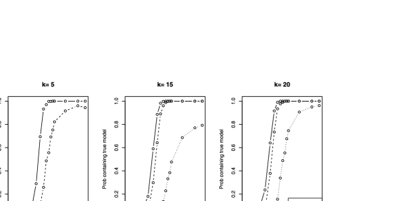
  Figure 1: Replication of the simulation setup considered in the discussion by Bühlmann et al., but now with attention being paid to correct variable screening, rather than exact variable recovery. Here, $k_{0}$ denotes the true number of nonzero coefficients, and $k$ the number of chosen lasso predictors (steps along the lasso path). We see that, with high probability, the true model is contained in the first 5, 15 or 20 chosen predictors.

  In any case, it is important to point out that the newer sequential testing procedure in Taylor et al. (2014) and the fixed-$\lambda$ testing procedure in Lee et al. (2013) do not assume a beta-min or irrepresentable condition whatsoever, and do not require any conditions like $\mathbb{P}(B)\rightarrow 1$.

Now we respond to some of the other points raised. One of the remarks that we made after the main result in Theorem 3 of our original paper claims that this result can be extended to cover just the “strong” true variables (ones with large coefficients), and not necessarily the “weak” ones (with small coefficients). Bühlmann et al. comment that such an extension would likely require a “zonal” assumption, that bounds the number of small true coefficients, as in Bühlmann and Mandozzi (2013). As a matter of fact, we know a number of examples, with many small nonzero coefficients, for which the conclusions of Theorem 3 continue to hold. In any case, we emphasize that the newer sequential test of Taylor et al. (2014) does not need to make any assumption of this sort, and neither does the fixed-$\lambda$ test of Lee et al. (2013).

Properly interpreting the covariance test $p$-values, as Bühlmann et al. point out, can be tricky. But we believe this comes with the territory of a conditional test for adaptive regression, since the null hypothesis is random (and, as Bühlmann et al. note, is an unobserved event). Consider the wine dataset from Section 7.1 of our original paper as an example. Looking at the $p$-values in right panel of Table 5, one might be tempted to conclude from the $p$-value of 0.173 in the fourth line that the constructed lasso model with alcohol, volatile acidity and sulphates contains all of the truly active variables. There are potentially several problems with such an interpretation (one of which being that we have no reason to believe that the true model here is actually linear), but we will focus on the most flagrant offense: because the constructed lasso model is random, the $p$-value of 0.173 reflects the test of a random null hypothesis, and so we cannot generally use it to draw conclusions about the specific variables alcohol, volatile acidity, sulphates that happened to have been selected in the current realization. The $p$-value of 0.173 does, however, speak to the significance of the 3-step lasso model, that is, the lasso model after 3 steps along the lasso path—said differently, we can think of this $p$-value as reflecting the significance of the 3 “most important” variables as deemed by the lasso. This properly accounts for the random nature of the hypothesis (as in any realization, the identity of these first 3 active variables may change), and is an example of valid post-selection inference.

Of course, one may ask: is this really what should be tested? That is, instead of inquiring about the significance of the 3-step lasso procedure, would a practitioner not actually want to know about the significance of the variables alcohol, volatile acidity and sulphates in particular? In a sense, this is really a question of philosophy, and the answer is not clear in our minds. Here, though, is a possibly helpful observation: when we consider a single wine data set, testing the significance of the (fixed) variables alcohol, volatile acidity and sulphates (after these 3 have been selected as active by the lasso) seems more natural; but when we consider a sequence of testing problems, in which we observe a new wine data set and rerun the lasso for 3 steps on each of a sequence of days $1,2,3,\ldots,$ testing the significance of the (random) 3-step lasso procedure seems more appropriate.

[As an important side note, in the finite sample spacing test given in Taylor et al. (2014), one can argue that both interpretations are valid, since our inference in this work is based on conditioning on the value of the selected variables.]

In Tables 1 and 2 of their discussion, Bühlmann et al. compare their approach to the covariance test in terms of false positive and false negative rates. In our original paper, we had not specified a sequential stopping rule for the covariance test, and it is not clear to us that the two they used were reasonable. (Additionally, we are not sure what form they assumed for the covariance test, as the representation they present, based on the difference in lasso criterion values, is not equivalent to the covariance statistic; see the first clarification bullet point above.) Bühlmann et al. kindly sent us their R code for their procedure, and we applied it to a subset of their examples, corresponding to the setup in the second row of each of their Tables 1 and 2. The results of 1000 simulations are shown in Table 1. There are two setups: $n=100$, $p=80$, and $n=100$, $p=200$. In line 1 of each, we applied their de-sparsification technique, using the same estimate of $\sigma$ as in their discussion. We found that this commonly overestimates $\sigma$ by $>$100%, so in line 2 we use the true value, $\sigma=1$. Line 3 uses the covariance test with the ForwardStop rule of Grazier G’Sell et al. (2013), and the true $\sigma=1$, designed to control the FDR at 5%. We see that the de-spars rule does well with the inflated estimate of $\sigma$, but produces far too many false positives when the true value of $\sigma$ is used. Reliance on a inflated variance estimate does not seem like a robust strategy, but perhaps there is a way to resolve this issue. (In all fairness, Bühlmann et al. told us that they are aware of this.) The covariance test with ForwardStop does a reasonable job of controlling the FDR, while capturing just under half of the true signals.

Table 1: Results of a simulation study, repeating the setup in the second row of each of Tables 1 and 2 from the Bühlmann et al. discussion. Shown are the average number of predictors called significant (out of $p=80$ or $200$), the average number of false and true positives, the familywise error rate and the false discovery rate

	Ave number called signif.	Ave FP	Ave TP	FWER	FDR
$n=100$, $p=80$
(1) de-spars (estimated $\sigma$)	06.89	00.05	6.84	0.04	0.01
(2) de-spars (true $\sigma$)	17.29	07.36	9.93	0.98	0.43
(3) covTest/forwStop	04.81	00.25	4.55	0.28	0.05
$n=100$, $p=200$
(1) de-spars (estimated $\sigma$)	03.35	00.04	3.30	0.04	0.01
(2) de-spars (true $\sigma$)	44.52	34.81	9.71	1.00	0.78
(3) covTest/forwStop	04.29	00.31	3.97	0.26	0.07

2 Interlude: Conditional or fixed hypothesis testing?

We would like to highlight some of the differences between conditional and fixed hypothesis testing. This section is motivated by the comments of Bühlmann et al., as well as the referees and Editors of our original article, and personal conversations with Larry Wasserman.

Though it has been said before, it is worth repeating: the covariance test does not give $p$-values for classic tests of fixed hypotheses, such as $\beta^{*}_{S}=0$ for a fixed subset $S\subseteq\{1,\ldots,p\}$; however, it was not designed for this purpose. As we see it: conditional hypothesis tests like the covariance test, and fixed hypothesis tests like that of van de Geer, Bühlmann and Ritov (2013) and many others (see the references in Section 2.5 of our original paper) are two principally different approaches for assessing significance in high-dimensional modeling. The motivation behind the covariance test and others is that often a practitioner becomes interested in assessing the significance of a variable only because it has been entered into the active set by a fitting procedure like the lasso. If this matches the actual workflow of the practitioner, then the covariance test or other conditional tests seem to be best-suited to his or her needs. A resulting complexity is that interpretation here must be drawn out carefully (refer back to Section 1).

On the other hand, the idea behind fixed tests like that of Zhang and Zhang (2014), van de Geer, Bühlmann and Ritov (2013) and Javanmard and Montanari (2013), (or at least, a typical use case in our view) is to compute $p$-values for all fixed hypothesis $\beta_{j}^{*}=0$, $j=1,\ldots,p$, and then perform a multiple testing correction at the end to determine global variable significance. Even though the lasso may have been used to construct such $p$-values, the practitioner is to pay no attention to its output—in particular, to its active set. And of course, the final model output by this testing procedure (which contains the variables deemed significant) may or may not match the lasso active set. The appeal of this approach lies in the simplicity and transparency of its conclusions: each computed $p$-value is associated with a familiar, classical hypothesis test, $\beta_{j}^{*}=0$ for a fixed $j$. In fact, we too like this approach, as it is very direct. One drawback is that it is unclear how this might be used for post-selection inference, if that is what is desired by the practitioner.

We note the conditional perspective is not really a foreign one, as it is indeed completely analogous to the (proper) interpretation of cross-validation errors for the lasso or forward stepwise regression. In this setting, to estimate the expected test error of a $k$-step model computed by, say, the lasso, we rerun the lasso for $k$ steps on a fraction of the data set, record the observed validation error on held-out data, and repeat this a number of times. This yields a final estimate of the expected test error for the $k$-step lasso model; but importantly, in each iteration of cross-validation, the selected variables will likely have changed (since the lasso is being run on different data sets), and so it is really only appropriate to regard cross-validation as producing as error estimate for the $k$-step lasso procedure, not for the particular realized model of size $k$ that was fit on the entire data set.

Lastly, we draw attention to a connection between our work on post-selection inference, and the de-biasing techniques pursued by Zhang and Zhang (2014), van de Geer, Bühlmann and Ritov (2013) and Javanmard and Montanari (2013). In Section 7.1 of Lee et al. (2013), we show how the framework developed in this paper can be used to form intervals or tests for the components of a de-biased version of the true coefficient vector, that is, something like a population analog of the de-biased estimator studied by these authors. Under the appropriate sufficient conditions [e.g., the same as those in Javanmard and Montanari (2013)], these population de-biased coefficients converge to the true ones, so these tests and intervals are also valid for the underlying coefficients as well.

3 Buja and Brown.

We thank Professors Buja and Brown for their scholarly summary of inference in adaptive regression. We learned a great deal from it and we enthusiastically recommend it to readers. They discuss in detail the forward stepwise approach, and outline many different ways to carry out inference in this setting. To explore the $t_{\max}$ proposal in their discussion, we carried out a simulation study. It turns out that this is helpful in illustrating the special properties of the covariance test with null distribution $\operatorname{Exp}(1/k)$, as well as the spacing $p$-values [Taylor et al. (2014)].

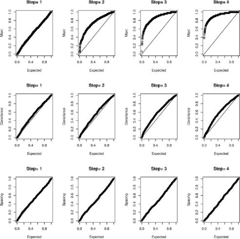
Figure 2: Simulation of $p$-values for the first four steps of using the test in (2) with forward stepwise regression (top row), the covariance test (middle row), and the spacing test (bottom row). Details are given in the text.

With $n=50$, $p=10$, we generated standardized Gaussian predictors, the population correlation between predictors $j$ and $j^{\prime}$ being $0.5^{|j-j^{\prime}|}$. The true coefficients were $\beta^{*}=0$, and the marginal error variance was $\sigma^{2}=1$. The middle and bottom panels of Figure 2 show quantile–quantile plots of the covariance $p$-values and spacing $p$-values for the first four steps of the least angle regression path [see (1) for the spacing test in the first step, and Taylor et al. (2014) for subsequent steps]. In the top panel, we have applied forward stepwise regression, using the test statistic

$$t_{\max}(y)=\max_{j=k,\ldots,p}\bigl{|}t^{(j)}(y)\bigr{|}\qquad\mbox{where }t^{(j)}(y)=\frac{\langle X_{j\cdot A},y\rangle}{\|X_{j\cdot A}\|_{2}},$$ (2)

per the proposal of Buja and Brown. Here, $A$ is the set of active variables currently in the model and $X_{j\cdot A}$ denotes the $j$th predictor orthogonalized with respect to these variables. Note that we have used the true value $\sigma^{2}=1$ in (2) (and in the covariance and spacing tests as well). As suggested by Buja and Brown, we simulated $\varepsilon\sim N(0,I)$ in order to estimate the $p$-value $\mathbb{P}(t_{\max}(\varepsilon)>t_{\max}(y))$.

All three tests look good at the first step, but the forward stepwise test based on (2) becomes more and more conservative for later steps. The reason is that the covariance test and the spacing test (even moreso) properly account for the selection events up to and including step $k$. To give a concrete example, the forward stepwise test ignores the fact that at the second step, the observed $t_{\max}$ is the second largest value of the statistic in the data, and erroneously compares it to a null distribution of largest $t_{\max}$ values. This creates a conservative bias in the $p$-value. If predictor $j$ were chosen at the first step of the forward stepwise procedure, then a correct numerical simulation for $t_{\max}$ at the second step would generate $y^{*}=X_{j}\hat{\beta}_{j}+\varepsilon$ (with $\hat{\beta}_{j}$ being the least squares coefficient on variable $j$), and only keep those $y^{*}$ vectors for which predictor $j$ is chosen at the first step, using these to compute $t_{\max}(y^{*})$ [which equals $t_{\max}(\varepsilon)$]. Such a simulation setup might be practical for a few steps, but would not be practical beyond that, though there do exist efficient algorithms for sampling from such distributions. Remarkably, the covariance and spacing tests are able carry out this conditioning analytically.

On a separate point, we agree with Buja and Brown that inferences should not typically focus on the true regression coefficients when predictors are highly correlated, and even the definition of FDR seems debatable in that setting. In Grazier G’Sell, Hastie and Tibshirani (2013), we propose an alternative definition of FDR, called the “Uninformative Variable Rate” (UVR), which tries to finesse this issue by projecting the true mean $X\beta^{*}$ onto the set of predictors in the current model. A selection is deemed a false positive if it has a zero coefficient in this projection. For example, in a model with $\beta_{1}^{*}=5$, $\beta^{*}_{2}=0$ and $\operatorname{Cor}(X_{1},X_{2})=0.95$, the selection of $X_{2}$ by itself would be considered a false positive in computing the FDR. But this does not seem reasonable, and the UVR would instead consider it a true positive.

As Buja and Brown mentioned, we have proposed a method for combining sequential $p$-values to achieve FDR control in Grazier G’Sell et al. (2013). But we believe there is more to do, especially in light of the last point just raised.

Finally, as they remark, our tests will not be valid if the practitioner uses them in combination with other selection techniques, or as they put it, the data analyst is “arbitrarily informal in their meta-selection of variable selection methods.” As they point out, the POSI methods they propose in Berk et al. (2013) are valid even in that situation. This is a very nice property, but of course the pressing question is: are the inferences too conservative as a result of protecting the type I error in such a broad sense?

4 Cai and Yuan.

We are grateful to Professors Cai and Yuan for their suggestion of an alternative test based on the Gumbel distribution. In the most basic setting, testing at the first step (i.e., global null hypothesis) in the orthogonal $X$ setting, both our proposal and theirs stem from the same basic arguments. To see this, suppose that $V_{1}\geq\cdots\geq V_{p}>0$ are the ordered absolute values of a sample from a standard normal distribution. Then, as $p\to\infty$,

$$b_{p}(V_{1}-a_{p})\stackrel{{\scriptstyle d}}{{\rightarrow}}\operatorname{Gumbel}(0,1),$$ (3)

where

$$a_{p}=\Phi^{-1}\bigl{(}1-1/(2p)\bigr{)}=\sqrt{2\log p}-\frac{\log\log p+\log\pi}{2\sqrt{2\log p}}+o(1/\sqrt{\log p})$$

and

$$b_{p}=\sqrt{2\log p}\bigl{(}1+o(1)\bigr{)}.$$

We used this and the fact that $b_{p}(V_{1}-V_{2})\stackrel{{\scriptstyle d}}{{\rightarrow}}\operatorname{Exp}(1)$ to handle the orthogonal $X$ case. Dividing (3) by $b_{p}^{2}$, we see that

$$\frac{V_{1}+a_{p}}{b_{p}}=\frac{V_{1}-a_{p}}{b_{p}}+2+o(1)\rightarrow 2$$

and multiplying by (3), we get

$$V_{1}^{2}-a_{p}^{2}\stackrel{{\scriptstyle d}}{{\rightarrow}}\operatorname{Gumbel}(0,2),$$

which may be rearranged to give Cai and Yuan’s observation [since $a_{p}^{2}=2\log p-\log\log p-\log\pi+o(1)$]. Hence for the orthogonal case, under the global null, we are basically using the same extreme value theory.

But for a general predictor matrix $X$, even if we stick to testing at the first step, we believe the Gumbel test does not share the same kind of parameter-free asymptotic behavior of the covariance test. Specifically, take $X^{T}X$ to be the $p\times p$ matrix with 1 on the diagonal and every off diagonal element equal to some fixed $\rho\in(0,1)$. In this case, we can show that under the global null,

$$V_{1}-\sqrt{2\rho\log p}\stackrel{{\scriptstyle d}}{{\rightarrow}}\bigl{|}N(0,1-\rho)\bigr{|},$$

so the asymptotic distribution depends on $\rho$, and the procedure suggested by Cai and Yang must fail. Figure 3 shows an example with $n=100$, $p=50$, and $\rho=0.7$. The Gumbel approximation is poor, while the $\operatorname{Exp}(1)$ distribution for the covariance test statistic still works well.

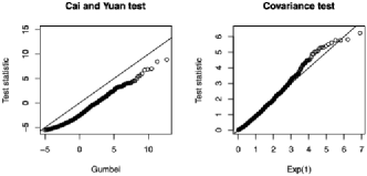
Figure 3: Quantile–quantile of Gumbel test (left panel) and covariance test (right panel) with features having pairwise correlation $0.7$.

Another important point is that, for a general $X$, the test proposed by Cai and Yuan does not apply to the sequence of variables entered along the lasso path. Cai and Yuan assume that, given a current active set $A$, the variable $j$ to be entered is that which maximizes the drop in residual sum of squares. (In their notation, the representation $R_{j}=\max_{m\notin A}R_{m}$ is what allows them to derive the asymptotic Gumbel null distribution for their test.) While this is true at each lasso step in the orthogonal $X$ case, it is certainly not true in the general $X$ case. Meanwhile, for an arbitrary $X$, it is true in forward stepwise regression (by definition).

5 Fan and Ke.

Professors Fan and Ke extend the covariance test and its null distribution to the SCAD and MCP penalties, in the orthogonal $X$ case. This is very exciting. We wonder whether this can be extended to arbitrary $X$, and whether the spacing test [Taylor et al. (2014)] can be similarly generalized.

Fan and Ke (and also Bühlmann, Meier and van de Geer) also study the important issue of the power of the covariance test, relative to the “RSSdrop” and “MaxCov” statistics. The discussants here have honed in on the worst case scenario for the covariance test, in which two predictors have large and equal coefficients. In this situation, the LARS algorithm takes only a short step after the first predictor has been entered, before entering the second predictor, and the hence the $p$-value for the first step is not very small. For this reason, better power can be achieved by constructing functions of more than one covariance test $p$-value, as illustrated by Figure 4 in the discussion of Fan and Ke. We note, however, that neither RSSdrop nor MaxCov have tractable null distributions in the general $X$ case, and it is not even clear how to approximate these null distributions by simulation except in the global null setup. Power concerns were also part of the motivation for our development of the sequential tests in Grazier G’Sell et al. (2013). Also, it is worth mentioning that the framework of Taylor et al. (2014) actually allows for combinations of the knots $\lambda_{j}$, $j=1,\ldots,k$ from the first $k$ steps, so that we could form an exact test based on, for example, $\sum_{j=1}^{k}\lambda_{j}$ is this was seen to have better power. Overall, the issue of the “most powerful sequential test” remains an open and important one.

Continuing on the topic of power, Fan and Ke (and again, Bühlmann et al.) raise asymptotic concerns. They suggest that power against coefficients on the order $O(n^{-1/2})$ is desirable. A first clarification: if elements of $y$ and the rows of $X$ are generated by i.i.d. sampling, then the matrix $X^{T}X$ grows like $n$; our standardization, in which $X^{T}X$ has 1 in each diagonal entry, corresponds to multiplying $\beta^{*}$ by $\sqrt{n}$ in this i.i.d. sampling context. The rate $O(n^{-1/2})$ mentioned then becomes $O(1)$. Power results will generally depend on $X$, and a complete discussion would be outside of the scope of this discussion, but some insight into what is possible or what is reasonable to expect may be gained by considering the orthogonal case. Consider now the problem of testing the global null against the alternative $\beta^{*}_{j_{0}}\neq 0$ and $\beta^{*}_{j}=0$ for all $j\neq j_{0}$, with $j_{0}$ known. For $|\beta^{*}_{j_{0}}|=\nu$, fixed, we get nontrivial limiting power by rejecting if $|U_{j_{0}}|=|X_{j_{0}}^{T}y|>z_{\alpha/2}$, as usual. But realistically, ${j_{0}}$ will not be known and it will be sensible to ask about the average power over all ${j_{0}}\in\{1,\ldots,p\}$. The problem of testing $\beta^{*}=0$ against the hypothesis that there is a unique ${j_{0}}\in\{1,\ldots,p\}$ for which $\beta^{*}_{j_{0}}\neq 0$ is invariant under permutations of the entries in $U$. Let ${\mathcal{T}}_{p}$ denote the class of all permutation invariant tests $T(U)$; our test $T_{1}$ and any other tests which are functions of the order statistics of $U_{j}$, $j=1,\ldots,p$ are permutation invariant. Let $B_{p}(\nu)$ be the set of $\beta^{*}$ with exactly one nonzero entry satisfying $|\beta^{*}_{j}|\leq\nu$. We can prove that if $\nu_{p}$ is any sequence of constants with

$$\sqrt{2\log p}-\nu_{p}\to\infty,$$

then

$$\sup_{T\in{\mathcal{T}}_{p},\beta^{*}\in B_{p}(\nu_{p})}\bigl{|}\operatorname{Power}\bigl{(}T,\beta^{*}\bigr{)}-\operatorname{Level}(T)\bigr{|}\to 0.$$

For tests which are not permutation invariant, we can prove

$$\sup_{T,\beta^{*}\in B_{p}(\nu_{p})}\bigl{|}\operatorname{AveragePower}\bigl{(}T,\beta^{*}\bigr{)}-\operatorname{Level}(T)\bigr{|}\to 0,$$

where now AveragePower denotes, for a given $\beta^{*}\in B_{p}(\nu_{p})$, the average over the $p$ vectors obtained by permuting the entries of $\beta^{*}$. In other words, unless $\beta^{*}$ has an entry on the order of $\sqrt{2\log p}$, there is no permutation invariant way to distinguish the null from the alternative. On the other hand, if $a_{p}=\sqrt{2\log p}-\log(\log p)/(2\sqrt{2\log p})$ and

$$a_{p}(a_{p}-\nu_{p})\to-\infty,$$

then our test has limiting power 1 in this context. This $\sqrt{2\log p}$ rate, then, cannot be substantially improved in general. The same conclusion holds if $B_{p}(\nu)$ is replaced by the intersection of the $O(1)$ ball $\{\beta\dvtx\|\beta\|_{2}\leq\Delta\}$ with $\{\beta\dvtx|\bar{\beta}|\leq\varepsilon_{p}/\sqrt{p}\}$. Here $\Delta$ is any fixed constant, $\bar{\beta}=\sum_{j=1}^{p}\beta_{j}/p$, and $\varepsilon_{p}$ is any sequence shrinking to 0. Notice that if $\beta^{*}$ in this set is known then using a likelihood ratio test against that alternative achieves nontrivial asymptotic power (provided $\|\beta^{*}\|_{2}$ stays away from 0). If the permutation group is expanded to the signed permutation group, then the condition on $\bar{\beta}$ may be deleted; natural procedures will have this added sign invariance in the orthogonal case.

6 Lv and Zheng.

Professors Lv and Zheng explore extensions of these ideas to nonconvex objective functions, for example, a combination of Lasso and the SICA penalty. This is interesting but seems difficult, as even the computation of the global solution is infeasible in general. However, the existing asymptotic results for these methods suggest that inference tools might also prove to be tractable. Regarding the significance of each active predictor conditional on the set of all remaining active predictors: the spacing theory in Taylor et al. (2014) provides a method for doing this.

Lv and Zheng also suggest extra shrinkage, replacing $\lambda_{k+1}$ in our, and their, test statistics by $c\lambda_{k+1}$, in the hopes that a better choice of $c<1$ will lead to an improved $\operatorname{Exp}(1)$ approximation. In knot form, this would look like

$$C(A,s_{A},j,s)\lambda_{k}(\lambda_{k}-c\lambda_{k+1})=T_{k}+(1-c)C(A,s_{A},j,s)\lambda_{k}\lambda_{k+1}.$$

Typically, $\lambda_{k}$, $\lambda_{k+1}$ are drifting to $\infty$ with $p$, so the shrinkage factor $c$ will have to be chosen carefully in order to control the second term above; it seems that $c\rightarrow 1$ is needed whenever the limit of $T_{k}$ is $\operatorname{Exp}(1)$.

7 Wasserman.

Professor Wasserman appropriately points out the stringency of assumptions made in our paper, assumptions that are common to much of the theoretical work on high-dimensional regression. We would like to reiterate that three of the offending assumptions in his list—that is, the assumptions that the true model is linear and is furthermore sparse, and that the predictors in $X$ are weakly correlated—are not needed in the newer works of Taylor et al. (2014) and Lee et al. (2013). In general, though, we do agree that the rest of assumptions in his list (implying independent, normal, homoskedastic errors) are used for as a default starting point for theoretical analysis, but are certainly suspect in practice.

Wasserman outlines a model-free approach to inference in adaptive regression based on sample-splitting and the increase in predictive risk due to setting a coefficient to zero. The proposal is simple and natural, and we can appreciate model-free approaches that use sample splitting like this one. However, we worry about the loss in power due to splitting the data in half, especially when $n$ is small relative to $p$. As he says, this may be the price to pay for added robustness to model misspecification. How steep is this price? It would be interesting to investigate, both theoretically or empirically, the precise power lost due to sample splitting. Also, we note that the random choice of splits will also influence the results, perhaps considerably. Therefore, one would need to take multiple random splits, and somehow combine the results at the end; but then the interpretation of the final “conditional” test seems challenging. We are eager to read a completed manuscript on this interesting idea.

His discussion of conformal prediction is fascinating; this is an area completely new to us. And finally, we thank him for his clearly expressed reminder of the difficulties of determining causality from a standard statistical model.

8 Thanks.

We thank all the discussants again for their contributions. They have given us much to think about. We hope that our original paper, the subsequent discussions and this response will be a valuable resource for researchers interested in inference for adaptive regression.

References

- Berk et al. (2013) {barticle}[mr] \bauthor\bsnmBerk, \bfnmRichard\binitsR., \bauthor\bsnmBrown, \bfnmLawrence\binitsL., \bauthor\bsnmBuja, \bfnmAndreas\binitsA., \bauthor\bsnmZhang, \bfnmKai\binitsK. and \bauthor\bsnmZhao, \bfnmLinda\binitsL. (\byear2013). \btitleValid post-selection inference. \bjournalAnn. Statist. \bvolume41 \bpages802–837. \biddoi=10.1214/12-AOS1077, issn=0090-5364, mr=3099122 \bptokimsref\endbibitem
-
Bühlmann and Mandozzi (2013)
{bmisc}[auto:STB—2014/02/12—14:17:21]
\bauthor\bsnmBühlmann, \bfnmP.\binitsP. and \bauthor\bsnmMandozzi, \bfnmJ.\binitsJ.
(\byear2013).
\bhowpublishedHigh-dimensional variable screening and bias in
subsequent inference,
with an empirical comparison. Comput. Statist.
DOI \doiurl10.1007/
s00180-013-0436-3. \bptokimsref\endbibitem - Grazier G’Sell, Hastie and Tibshirani (2013) {bmisc}[auto:STB—2014/02/12—14:17:21] \bauthor\bsnmGrazier G’Sell, \bfnmM.\binitsM., \bauthor\bsnmHastie, \bfnmT.\binitsT. and \bauthor\bsnmTibshirani, \bfnmR.\binitsR. (\byear2013). \bhowpublishedFalse variable selection rates in regression. Preprint. Available at \arxivurlarXiv:1302.2303. \bptokimsref\endbibitem
- Grazier G’Sell et al. (2013) {bmisc}[auto:STB—2014/02/12—14:17:21] \bauthor\bsnmGrazier G’Sell, \bfnmM.\binitsM., \bauthor\bsnmWager, \bfnmS.\binitsS., \bauthor\bsnmChouldechova, \bfnmA.\binitsA. and \bauthor\bsnmTibshirani, \bfnmR.\binitsR. (\byear2013). \bhowpublishedFalse discovery rate control for sequential selection procedures, with application to the lasso. Preprint. Available at \arxivurlarXiv:1309.5352. \bptokimsref\endbibitem
- Javanmard and Montanari (2013) {bmisc}[auto:STB—2014/02/12—14:17:21] \bauthor\bsnmJavanmard, \bfnmA.\binitsA. and \bauthor\bsnmMontanari, \bfnmA.\binitsA. (\byear2013). \bhowpublishedConfidence intervals and hypothesis testing for high-dimensional regression. Preprint. Available at \arxivurlarXiv:1306.3171. \bptokimsref\endbibitem
- Lee et al. (2013) {bmisc}[auto:STB—2014/02/12—14:17:21] \bauthor\bsnmLee, \bfnmJ.\binitsJ., \bauthor\bsnmSun, \bfnmD.\binitsD., \bauthor\bsnmSun, \bfnmY.\binitsY. and \bauthor\bsnmTaylor, \bfnmJ. E.\binitsJ. E. (\byear2013). \bhowpublishedExact inference after model selection via the lasso. Preprint. Available at \arxivurlarXiv:1311.6238. \bptokimsref\endbibitem
- Taylor, Loftus and Tibshirani (2013) {bmisc}[auto:STB—2014/02/12—14:17:21] \bauthor\bsnmTaylor, \bfnmJ.\binitsJ., \bauthor\bsnmLoftus, \bfnmJ.\binitsJ. and \bauthor\bsnmTibshirani, \bfnmR. J.\binitsR. J. (\byear2013). \bhowpublishedTests in adaptive regression via the Kac–Rice formula. Preprint. Available at \arxivurlarXiv:1308.3020. \bptokimsref\endbibitem
- Taylor et al. (2014) {bmisc}[auto:STB—2014/02/12—14:17:21] \bauthor\bsnmTaylor, \bfnmJ.\binitsJ., \bauthor\bsnmLockhart, \bfnmR.\binitsR., \bauthor\bsnmTibshirani, \bfnmR. J.\binitsR. J. and \bauthor\bsnmTibshirani, \bfnmR.\binitsR. (\byear2014). \bhowpublishedPost-selection adaptive inference for least angle regression and the lasso. Preprint. Available at \arxivurlarXiv:1401.3889. \bptokimsref\endbibitem
- van de Geer, Bühlmann and Ritov (2013) {bmisc}[auto] \bauthor\bsnmvan de Geer, \bfnmSara\binitsS., \bauthor\bsnmBühlmann, \bfnmPeter\binitsP. and \bauthor\bsnmRitov, \bfnmY.\binitsY. (\byear2013). \bhowpublishedOn asymptotically optimal confidence regions and tests for high-dimensional models. Preprint. Available at \arxivurlarXiv:1303.0518. \bptokimsref\endbibitem
- Zhang and Zhang (2014) {barticle}[auto:STB—2014/02/12—14:17:21] \bauthor\bsnmZhang, \bfnmC.-H.\binitsC.-H. and \bauthor\bsnmZhang, \bfnmS.\binitsS. (\byear2014). \btitleConfidence intervals for low dimensional parameters in high dimensional linear models. \bjournalJ. R. Stat. Soc. Ser. B. Stat. Methodol. \bvolume76 \bpages217–242. \bidmr=3153940 \bptokimsref\endbibitem