Discussion: “A significance test for the lasso”

10.1214/13-AOS1175

Discussion of “A significance test for the lasso”

The paper by Lockhart, Taylor, Tibshirani and Tibshirani (LTTT) is an important advancement in our understanding of inference for high-dimensional regression. The paper is a tour de force, bringing together an impressive array of results, culminating in a set of very satisfying convergence results. The fact that the test statistic automatically balances the effect of shrinkage and the effect of adaptive variable selection is remarkable.

The authors make very strong assumptions. This is quite reasonable: to make significant theoretical advances in our understanding of complex procedures, one has to begin with strong assumptions. The following question then arises: what can we do without these assumptions?

1 The assumptions

The assumptions in this paper—and in most theoretical papers on high-dimensional regression—have several components. These include:

[(5)]

The linear model is correct.

The variance is constant.

The errors have a Normal distribution.

The parameter vector is sparse.

The design matrix has very weak collinearity. This is usually stated in the form of incoherence, eigenvalue restrictions or incompatibility assumptions.

To the best of my knowledge, these assumptions are not testable when $p>n$. They are certainly a good starting place for theoretical investigations but they are indeed very strong. The regression function $m(x)=\mathbb{E}(Y|X=x)$ can be any function. There is no reason to think it will be close to linear. Design assumptions are also highly suspect. High collinearity is the rule rather than the exception especially in high-dimensional problems. An exception is signal processing, in particular compressed sensing, where the user gets to construct the design matrix. In this case, if the design matrix is filled with independent random Normals, the design matrix will be incoherent with high probability. But this is a rather special situation.

None of this is meant as a criticism of the paper. Rather, I am trying to motivate interest in the question I asked earlier, namely: what can we do without these assumptions?

Remark 1.

It is also worth mentioning that even in low-dimensional models and even if the model is correct, model selection raises troubling issues that we all tend to ignore. In particular, variable selection makes the minimax risk explode [Leeb and Pötscher (2005, 2008)]. This is not some sort of pathological risk explosion, rather, the risk is large in a neighborhood of 0, which is a part of the parameter space we care about.

2 The assumption-free lasso

To begin it is worth pointing out that the lasso has a very nice assumption-free interpretation.

Suppose we observe $(X_{1},Y_{1}),\ldots,(X_{n},Y_{n})\sim P$ where $Y_{i}\in\mathbb{R}$ and $X_{i}\in\mathbb{R}^{d}$. The regression function $m(x)=\mathbb{E}(Y|X=x)$ is some unknown, arbitrary function. We have no hope to estimate $m(x)$ nor do we have licence to impose assumptions on $m$.

But there is sound theory to justify the lasso that makes virtually no assumptions. In particular, I refer to Greenshtein and Ritov (2004) and Juditsky and Nemirovski (2000).

Let ${\mathcal{L}}=\{x^{t}\beta\dvtx\beta\in\mathbb{R}^{d}\}$ be the set of linear predictors. For a given $\beta$, define the predictive risk

$$R(\beta)=E\bigl{(}Y-\beta^{T}X\bigr{)}^{2},$$

where $(X,Y)$ is a new pair. Let us define the best, sparse, linear predictor $\ell_{*}(x)=\beta_{*}^{T}x$ (in the $\ell_{1}$ sense) where $\beta_{*}$ minimizes $R(\beta)$ over the set $B(L)=\{\beta\dvtx\|\beta\|_{1}\leq L\}$. The lasso estimator $\hat{\beta}$ minimizes the empirical risk $\hat{R}(\beta)=\frac{1}{n}\sum_{i=1}^{n}(Y_{i}-\beta^{T}X_{i})^{2}$ over $B(L)$. For simplicity, I will assume that all the variables are bounded by $C$ (but this is not really needed). We make no other assumptions: no linearity, no design assumptions and no models. It is now easily shown that

$$R(\hat{\beta})\leq R(\beta_{*})+\sqrt{\frac{8C^{2}L^{4}}{n}\log\biggl{(}\frac{2p^{2}}{\delta}\biggr{)}}$$

except on a set of probability at most $\delta$.

This shows that the predictive risk of the lasso comes close to the risk of the best sparse linear predictor. In my opinion, this explains why the lasso “works.” The lasso gives us a predictor with a desirable property—sparsity—while being computationally tractable and it comes close to the risk of the best sparse linear predictor.

3 Interlude: Weak versus strong modeling

When developing new methodology, I think it is useful to consider three different stages of development: [(3)]

Constructing the method.

Interpreting the output of the method.

Studying the properties of the method. I also think it is useful to distinguish two types of modeling. In strong modeling, the model is assumed to be true in all three stages. In weak modeling, the model is assumed to be true for stage 1 but not for stages 2 and 3. In other words, one can use a model to help construct a method. But one does not have to assume the model is true when it comes to interpretation or when studying the theoretical properties of the method. My discussion is guided by my preference for weak modeling.

4 Assumption-free inference: The HARNESS

Here, I would like to discuss an approach I have been developing with Ryan Tibshirani. We call this: High-dimensional Agnostic Regression Not Employing Structure or Sparsity, or, the HARNESS. The method is a variant of the idea proposed in Wasserman and Roeder (2009).

The idea is to split the data into two halves. ${\mathcal{D}}_{1}$ and ${\mathcal{D}}_{2}$. For simplicity, assume that $n$ is even so that each half has size $m=n/2$. From the first half ${\mathcal{D}}_{1}$, we select a subset of variables $S$. The method is agnostic about how the variable selection is done. It could be forward stepwise, lasso, elastic net or anything else. The output of the first part of the analysis is the subset of predictors $S$ and an estimator $\hat{\beta}=(\hat{\beta}_{j}\dvtx j\in S)$. The second half of the data ${\mathcal{D}}_{2}$ is used to provide distribution-free inferences for the following questions: [(3)]

What is the predictive risk of $\hat{\beta}$?

How much does each variable in $S$ contribute to the predictive risk?

What is the best linear predictor using the variables in $S$? All the inferences from ${\mathcal{D}}_{2}$ are interpreted as being conditional on ${\mathcal{D}}_{1}$. (A variation is to use ${\mathcal{D}}_{1}$ only to produce $S$ and then construct the coefficients of the predictor from ${\mathcal{D}}_{2}$. For the purposes of this discussion, we use $\hat{\beta}$ from ${\mathcal{D}}_{1}$.)

In more detail, let

$$R=\mathbb{E}\bigl{|}Y-X^{T}\hat{\beta}\bigr{|},$$

where the randomness is over the new pair $(X,Y)$; we are conditioning on ${\mathcal{D}}_{1}$. Note that in this section I have changed the definition of $R$ to be on the absolute scale which is more interpretable. In the above equation, it is understood that $\hat{\beta}_{j}=0$ when $j\notin S$. The first question refers to producing a estimate and confidence interval for $R$ (conditional on ${\mathcal{D}}_{1}$). The second question refers to inferring

$$R_{j}=\mathbb{E}\bigl{|}Y-X^{T}\hat{\beta}_{(j)}\bigr{|}-\mathbb{E}\bigl{|}Y-X^{T}\hat{\beta}\bigr{|}$$

for each $j\in S$, where $\beta_{(j)}$ is equal to $\hat{\beta}$ except that $\hat{\beta}_{j}$ is set to 0. Thus, $R_{j}$ is the risk inflation by excluding $X_{j}$. The third question refers to inferring

$$\beta^{*}=\mathop{\arg\min}_{\beta\in\mathbb{R}^{k}}\mathbb{E}\bigl{(}Y-X_{S}^{T}\beta\bigr{)}^{2}$$

the coefficient of the best linear predictor for the chosen model. We call $\beta^{*}$ the projected parameter. Hence, $x^{T}\beta^{*}$ is the best linear approximation to $m(x)$ on the linear space spanned by the selected variables.

A consistent estimate of $R$ is

$$\hat{R}=\frac{1}{m}\sum_{i=1}^{m}\delta_{i},$$

where the sum is over ${\mathcal{D}}_{2}$, and $\delta_{i}=|Y_{i}-X_{i}^{T}\hat{\beta}|$. An approximate $1-\alpha$ confidence interval for $R$ is $\hat{R}\pm z_{\alpha/2}s/\sqrt{m}$ where $s$ is the standard deviation of the $\delta_{i}$’s.

The validity of this confidence interval is essentially distribution-free. In fact, if we want to be purely distribution-free and avoid asymptotics, we could instead define $R$ to be the median of the law of $|Y-X^{T}\hat{\beta}|$. Then the order statistics of the $\delta_{i}$’s can be used in the usual way to get a finite sample, distribution-free confidence interval for $R$.

Estimates and confidence intervals for $R_{j}$ can be obtained from $e_{1},\ldots,e_{m}$ where

$$e_{i}=\bigl{|}Y_{i}-X^{T}\hat{\beta}_{(j)}\bigr{|}-\bigl{|}Y_{i}-X^{T}\hat{\beta}\bigr{|}.$$

Estimates and confidence intervals for $\beta_{*}$ can be obtained by standard least squares procedures based on ${\mathcal{D}}_{2}$. The steps are summarized in Figure LABEL:figharness.

The HARNESS

The HARNESS bears some similarity to POSI [Berk et al. (2013)] which is another inference method for model selection. They both eschew any assumption that the linear model is correct. But POSI attempts to make inferences that are valid over all possible selected models while the HARNESS restricts attention to the selected model. Also, the HARNESS emphasizes predictive inferential statement.

Here is an example using the wine dataset. (Thanks to the authors for providing the data.) Using the first half of the data, we applied forward stepwise selection and used $C_{p}$ to select a model. The selected variables are Alcohol, Volatile_Acidity, Sulphates, Total_Sulfur_Dioxide and pH. A 95 percent confidence interval for the predictive risk of the null model is (0.65,0.70). For the selected model, the confidence interval for $R$ is (0.46,0.53). The (Bonferroni-corrected) 95 percent confidence intervals for the $R_{j}$’s are shown in the first plot of Figure 2. The (Bonferroni-corrected) 95 percent confidence intervals for the parameters of the projected model are shown in the second plot in Figure 2.

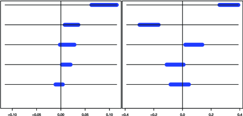
Figure 2: Left plot: confidence intervals for $R_{j}$. Right plot: confidence intervals for projected parameters. From top down the variables are Alcohol, Volatile_Acidity, Sulphates, Total_Sulfur_Dioxide and pH.

5 The value of data-splitting

Some statisticians are uncomfortable with data-splitting. There are two common objections. The first is that the inferences are random: if we repeat the procedure we will get different answers. The second is that it is wasteful.

The first objection can be dealt with by doing many splits and combining the information appropriately. This can be done but is somewhat involved and will be described elsewhere. The second objection is, in my view, incorrect. The value of data splitting is that leads to simple, assumption-free inference. There is nothing wasteful about this. Both halves of the data are being put to use. Admittedly, the splitting leads to a loss of power compared to ordinary methods if the model were correct. But this is a false comparison since we are trying to get inferences without assuming the model is correct. It is a bit like saying that nonparametric function estimators have slower rates of convergence than parametric estimators. But that is only because the parametric estimators invoke stronger assumptions.

6 Conformal prediction

Since I am focusing my discussion on regression methods that make weak assumptions, I would also like to briefly mention Vladimir Vovk’s theory of conformal inference. This is a completely distribution-free, finite sample method for predictive regression. The method is described in Vovk, Gammerman and Shafer (2005) and Vovk, Nouretdinov and Gammerman (2009). Unfortunately, most statisticians seem to be unaware of this work which is a shame. The statistical properties (such as minimax properties) of conformal prediction were investigated in Lei, Robins and Wasserman (2014), Lei and Wasserman (2014).

A full explanation of the method is beyond the scope of this discussion but I do want to give the general idea and say why it is related the current paper. Given data $(X_{1},Y_{1}),\ldots,(X_{n},Y_{n})$, suppose we observe a new $X$ and want to predict $Y$. Let $y\in\mathbb{R}$ be an arbitrary real number. Think of $y$ as a tentative guess at $Y$. Form the augmented data set

$$(X_{1},Y_{1}),\ldots,(X_{n},Y_{n}),(X,y).$$

Now we fit a linear model to the augmented data and compute residuals $e_{i}$ for each of the $n+1$ observations. Now we test $H_{0}\dvtx Y=y$. Under $H_{0}$, the residuals are invariant under permutations and so

$$p(y)=\frac{1}{n+1}\sum_{i=1}^{n+1}I\bigl{(}|e_{i}|\geq|e_{n+1}|\bigr{)}$$

is a distribution-free $p$-value for $H_{0}$.

Next, we invert the test: let $C=\{y\dvtx p(y)\geq\alpha\}$. It is easy to show that

$$\mathbb{P}(Y\in C)\geq 1-\alpha.$$

Thus, $C$ is distribution-free, finite-sample prediction interval for $Y$. Like the HARNESS, the validity of the method does not depend on the linear model being correct. The set $C$ has the desired coverage probability no matter what the true model is. Both the HARNESS and conformal prediction use the linear model as a device for generating predictions but neither requires the linear model to be true for the inferences to be valid. [In fact, in the conformal approach, any method of generating residuals can be used. It does not have to be a linear model. See Lei and Wasserman (2014).]

One can also look at how the prediction interval $C$ changes as different variables are removed. This gives another assumption-free method to explore the effects of predictors in regression. Minimizing the length of the interval over the lasso path can also be used as a distribution-free method for choosing the regularization parameter of the lasso.

On a related note, we might also be interested in assumption-free methods for the related task of inferring graphical models. For a modest attempt at this, see Wasserman, Kolar and Rinaldo (2013).

7 Causation

LTTT do not discuss causation. But in any discussion of the assumptions underlying regression, causation is lurking just below the surface. Indeed, there is a tendency to conflate causation and inference. To be clear: prediction, inference and causation are three separate ideas.

Even if the linear model is correct, we have to be careful how we interpret the parameters. Many articles and textbooks describe $\beta_{j}$ as the change in $Y$ if $X_{j}$ is changed, holding the other covariates fixed. This is incorrect. In fact, $\beta_{j}$ is the change in our prediction of $Y$ if $X_{j}$ is changed. This may seem like nit-picking but this is the very difference between association and causation.

Causation refers to the change in $Y$ as $X_{j}$ is changed. Association (prediction) refers to the change in our prediction of $Y$ as $X_{j}$ is changed. Put another way, prediction is about $\mathbb{E}(Y|\mbox{ observe }X=x)$ while causation is about $\mathbb{E}(Y|\mbox{ set }X=x)$. If $X$ is randomly assigned, they are the same. Otherwise, they are different. To make the causal claim, we have to include in the model, every possible confounding variable that could affect both $Y$ and $X$. This complete causal model has the form

$$Y=g(X,Z)+\varepsilon,$$

where $Z=(Z_{1},\ldots,Z_{k})$ represents all confounding variables in the world. The relationship between $Y$ and $X$ alone is described as

$$Y=f(X)+\varepsilon^{\prime}.$$

The causal effect—the change in $Y$ as $X_{j}$ is changed—is given by $\partial g(x,z)/\partial x_{j}$. The association (prediction)—the change in our prediction of $Y$ as $X_{j}$ is changed—is given by $\partial f(x)/\partial x_{j}$. If there are any omitted confounding variables, then these will be different.

Which brings me back to the paper. Even if the linear model is correct, we still have to exercise great caution in interpreting the coefficients. Most users of our methods are nonstatisticians and are likely to interpret $\beta_{j}$ causally no matter how many warnings we give.

8 Conclusion

LTTT have produced a fascinating paper that significantly advances our understanding of high-dimensional regression. I expect there will be a flurry of new research inspired by this paper.

My discussion has focused on the role of assumptions. In low-dimensional models, it is relatively easy to create methods that make few assumptions. In high-dimensional models, low assumption inference is much more challenging.

I hope I have convinced the authors that the low assumption world is worth exploring. In the meantime, I congratulate the authors on an important and stimulating paper.

References

- Berk et al. (2013) {barticle}[mr] \bauthor\bsnmBerk, \bfnmRichard\binitsR., \bauthor\bsnmBrown, \bfnmLawrence\binitsL., \bauthor\bsnmBuja, \bfnmAndreas\binitsA., \bauthor\bsnmZhang, \bfnmKai\binitsK. and \bauthor\bsnmZhao, \bfnmLinda\binitsL. (\byear2013). \btitleValid post-selection inference. \bjournalAnn. Statist. \bvolume41 \bpages802–837. \biddoi=10.1214/12-AOS1077, issn=0090-5364, mr=3099122 \bptokimsref\endbibitem
- Greenshtein and Ritov (2004) {barticle}[mr] \bauthor\bsnmGreenshtein, \bfnmEitan\binitsE. and \bauthor\bsnmRitov, \bfnmYa’acov\binitsY. (\byear2004). \btitlePersistence in high-dimensional linear predictor selection and the virtue of overparametrization. \bjournalBernoulli \bvolume10 \bpages971–988. \biddoi=10.3150/bj/1106314846, issn=1350-7265, mr=2108039 \bptokimsref\endbibitem
- Juditsky and Nemirovski (2000) {barticle}[mr] \bauthor\bsnmJuditsky, \bfnmAnatoli\binitsA. and \bauthor\bsnmNemirovski, \bfnmArkadii\binitsA. (\byear2000). \btitleFunctional aggregation for nonparametric regression. \bjournalAnn. Statist. \bvolume28 \bpages681–712. \biddoi=10.1214/aos/1015951994, issn=0090-5364, mr=1792783 \bptokimsref\endbibitem
- Leeb and Pötscher (2005) {barticle}[mr] \bauthor\bsnmLeeb, \bfnmHannes\binitsH. and \bauthor\bsnmPötscher, \bfnmBenedikt M.\binitsB. M. (\byear2005). \btitleModel selection and inference: Facts and fiction. \bjournalEconometric Theory \bvolume21 \bpages21–59. \biddoi=10.1017/S0266466605050036, issn=0266-4666, mr=2153856 \bptokimsref\endbibitem
- Leeb and Pötscher (2008) {barticle}[mr] \bauthor\bsnmLeeb, \bfnmHannes\binitsH. and \bauthor\bsnmPötscher, \bfnmBenedikt M.\binitsB. M. (\byear2008). \btitleSparse estimators and the oracle property, or the return of Hodges’ estimator. \bjournalJ. Econometrics \bvolume142 \bpages201–211. \biddoi=10.1016/j.jeconom.2007.05.017, issn=0304-4076, mr=2394290 \bptokimsref\endbibitem
- Lei, Robins and Wasserman (2014) {bmisc}[auto:STB—2014/02/12—14:17:21] \bauthor\bsnmLei, \bfnmJ.\binitsJ., \bauthor\bsnmRobins, \bfnmJ.\binitsJ. and \bauthor\bsnmWasserman, \bfnmLarry\binitsL. (\byear2013). \bhowpublishedDistribution-free prediction sets. J. Amer. Statist. Assoc. 108 278–287. \bptokimsref\endbibitem
- Lei and Wasserman (2014) {bmisc}[auto:STB—2014/02/12—14:17:21] \bauthor\bsnmLei, \bfnmJ.\binitsJ. and \bauthor\bsnmWasserman, \bfnmLarry\binitsL. (\byear2014). \bhowpublishedDistribution-free prediction bands for non-parametric regression. J. R. Stat. Soc. Ser. B. 76 71–96. \bptokimsref\endbibitem
- Vovk, Gammerman and Shafer (2005) {bbook}[mr] \bauthor\bsnmVovk, \bfnmVladimir\binitsV., \bauthor\bsnmGammerman, \bfnmAlexander\binitsA. and \bauthor\bsnmShafer, \bfnmGlenn\binitsG. (\byear2005). \btitleAlgorithmic Learning in a Random World. \bpublisherSpringer, \blocationNew York. \bidmr=2161220 \bptokimsref\endbibitem
- Vovk, Nouretdinov and Gammerman (2009) {barticle}[mr] \bauthor\bsnmVovk, \bfnmVladimir\binitsV., \bauthor\bsnmNouretdinov, \bfnmIlia\binitsI. and \bauthor\bsnmGammerman, \bfnmAlex\binitsA. (\byear2009). \btitleOn-line predictive linear regression. \bjournalAnn. Statist. \bvolume37 \bpages1566–1590. \biddoi=10.1214/08-AOS622, issn=0090-5364, mr=2509084 \bptokimsref\endbibitem
- Wasserman, Kolar and Rinaldo (2013) {bmisc}[auto:STB—2014/02/12—14:17:21] \bauthor\bsnmWasserman, \bfnmL.\binitsL., \bauthor\bsnmKolar, \bfnmM.\binitsM. and \bauthor\bsnmRinaldo, \bfnmA.\binitsA. (\byear2013). \bhowpublishedEstimating undirected graphs under weak assumptions. Preprint. Available at \arxivurlarXiv:1309.6933. \bptokimsref\endbibitem
- Wasserman and Roeder (2009) {barticle}[mr] \bauthor\bsnmWasserman, \bfnmLarry\binitsL. and \bauthor\bsnmRoeder, \bfnmKathryn\binitsK. (\byear2009). \btitleHigh-dimensional variable selection. \bjournalAnn. Statist. \bvolume37 \bpages2178–2201. \biddoi=10.1214/08-AOS646, issn=0090-5364, mr=2543689 \bptokimsref\endbibitem