Quantum and Classical Superballistic Transport in a Relativistic Kicked-Rotor System

Abstract

As an unusual type of anomalous diffusion behavior, superballistic transport is not well known but has been experimentally simulated recently. Quantum superballistic transport models to date are mainly based on connected sublattices which are constructed to have different properties. In this work, we show that both quantum and classical superballistic transport in the momentum space can occur in a simple periodically driven Hamiltonian system, namely, a relativistic kicked-rotor system with a nonzero mass term. The nonzero mass term essentially realizes a junction-like scenario: regimes with low or high momentum values have different dispersion relations and hence different transport properties. It is further shown that the quantum and classical superballistic transport should occur under much different choices of the system parameters. The results are of interest to studies of anomalous transport, quantum and classical chaos, and the issue of quantum-classical correspondence.

I Introduction

The rich transport behavior in complex systems is an important research topic in statistical physics review1 ; review2 ; review3 ; review4 ; PRLbarkai ; exponential . Consider the mean square of a physical quantity (such as position) as a function of time $t$ for an ensemble of particles. For normal diffusion, this mean quantity is proportional to $t$; whereas for anomalous diffusion, the mean quantity goes like $\sim t^{\nu}$ ($\nu\neq 1$), with subdiffusion referring to cases of $0<\nu<1$ and superdiffusion referring to cases of $1<\nu<2$. In the classical domain, known examples of anomalous diffusion include Brownian motion and heat conduction. In the quantum domain, wavepacket spreading in a periodic potential leads to ballistic transport in the mean square position ($\nu=2$). By contrast, wavepacket spreading in a quasi-periodic potential often induces subdiffusion or superdiffusion abe ; piechon ; ketzmerick .

The special class of diffusion with $\nu>2$, which may be termed as “superballistic transport”, is however not as well-studied as other cases of anomalous transport behavior. In the classical domain, superballistic transport was observed for Brownian particles Bao2007 ; Siegle2010 . In the quantum case, a time-dependent random potential was demonstrated to cause superballistic transport using paraxial optical setting Levi2012 . More related to this work, earlier superballistic transport was found in the dynamics of wavepacket spreading in a tight-binding lattice junction Hufnagel2001 ; Zhenjun2012 . Remarkably, such type of quantum superballistic transport was recently experimentally realized by use of optical wave packets in a designed hybrid photonic lattice setup Stutzer2013 .

The main objective of this work is to use a relatively simple model system to better understand the difference and connection between quantum and classical superballistic transport in purely Hamiltonian systems. To our knowledge, the model studied in this work represents the only dynamical model that can possess superballistic transport in both quantum and classical Hamiltonian dynamics. This will shed more light on various mechanisms of superballistic transport as well as on the general issue of quantum dynamics in classically chaotic systems. Further studies regarding the subtle correspondence between quantum and classical superballistic transport can be also motivated.

Specifically, we consider a relativistic variant  Chernikov1989 ; Matrasulov2005 of the well-known kicked-rotor (KR) model CasatiBook1995 and reveal the quantum and classical superballistic transport dynamics in the momentum space. Such a system can be also regarded as a periodically driven Dirac system, and it should be of some experimental interest due to recent advances in the quantum simulation of Dirac-like particles. In the massless case in which the kinetic energy of a relativistic particle is a linear function of momentum, the relativistic KR variant was known as the “Maryland model”, first investigated by Grempel et. al Grempel1982 ; Prange1984 , Berry Berry1984 and Simon Simon1985 to analytically understand the issue of Anderson localization. For a Dirac particle with a nonzero mass, the bare dispersion relation now lies between linear and quadratic: for low momentum values the dispersion is almost quadratic and for very high momentum values the dispersion approaches a linear function. In effect, this realizes a situation, now in the momentum space, in which two (momentum) sublattices with different dispersion relations (and hence different nature of on-site potential) are connected as a junction Hufnagel2001 . As shown later, this indeed induces superballistic transport in both the classical and quantum dynamics. Interestingly, the detailed mechanism in the former is still markedly different from that in the latter. In particular, in the classical case, it is necessary to break the global KAM curves in the classical phase space because the superballistic transport roots in an unusually complicated escape from a phase space regime of random motion to a simple ballistic structure. By contrast, in the quantum case, breaking global KAM curves are not essential for quantum superballistic transport to occur thanks to quantum tunneling through the KAM curves.

This paper is organized as follows. In Sec. II, we introduce our model and discuss its relation with the well-known Maryland model. In Sec. III we study quantum superballistic dynamics, followed by a parallel study of classical superballistic transport and the associated classical phase space structure in Sec. IV. Section V concludes this work.

II Relativistic Kicked Rotor as a Driven Dirac System

Consider a one-dimensional relativistic quantum KR Matrasulov2005 :

$$H=2\pi\alpha\hat{p}\sigma_{x}+M\sigma_{z}+K\cos(q{\theta})\sum_{n=-\infty}^{+\infty}{\delta(t-n)},$$ (1)

where all the variables are scaled and hence in dimensionless units. Here $\sigma_{x}$ and $\sigma_{z}$ are Pauli matrices, $v=2\pi\alpha$ represents the speed of light, $M$ represents the static mass energy, $K$ represents the strength of a delta-kicking field that is $(2\pi/q)$-periodic in the coordinate $\theta$ ($q$ is an integer) and unity-periodic in time, $\hat{p}=-i\hbar_{\text{eff}}\frac{\partial}{\partial\theta}$, where $\hbar_{\text{eff}}$ is a dimensionless effective Planck constant.

In the case of a vanishing $M$, the Hamiltonian (1) can be decoupled into two independent Hamiltonians, each associated with one eigen-spinor of $\sigma_{x}$. They are nothing but the so-called Maryland model  Grempel1982 :

$$H_{M}=\pm 2\pi\alpha\hat{p}+K\cos(q{\theta})\sum_{n=-\infty}^{+\infty}{\delta(t-n)}.$$ (2)

Early studies on this massless relativistic KR Grempel1982 ; Berry1984 investigated the consequences of rational or irrational values of $\alpha$. Indeed, by mapping the Maryland model onto a one-dimensional Anderson model, it becomes clear that $H_{M}$ with an irrational $\alpha$ should display Anderson localization in the momentum space Grempel1982 , whereas $H_{M}$ with a rational $\alpha=r/s$ ($r$ and $s$ integers) should show ballistic transport, so long as the parameter $q$ in the kicking potential is an integer multiple of $s$ Berry1984 . This condition is called a resonance condition. When this resonance condition is not fulfilled, i.e., $q\neq ns$, it can be shown that the time-evolving wavefunction of the system (with rational $\alpha$) repeats itself after every $s$ kicking periods, so neither Anderson localization nor ballistic transport occurs. Roughly speaking, what is known in the standard quantum KR CasatiBook1995 applies also here, concerning the importance of the arithmetic nature of $\alpha$ for the dynamics of the Maryland model, as well as the ballistic transport due to quantum resonances therein.

Though in this work we will focus on cases with a nonzero $M$, the above-mentioned results for the Maryland model do guide us when it comes to choose interesting parameter regimes. For example, we shall pay special attention to whether or not $\alpha$ is a rational value, and if the kicking potential is resonant or not. As it turns out, the quantum dynamics is most interesting in cases with rational $\alpha$ and under the resonance condition.

Since our model is a periodically driven system, we write down its Floquet operator in the $\theta$-representation, i.e., the propagator associated with one-period time evolution:

$${U}=e^{-i\frac{1}{\hbar_{\text{eff}}}(2\pi\alpha\sigma_{x}\hat{p}+\sigma_{z}M)}e^{-i\frac{K}{\hbar_{\text{eff}}}\cos(q{\theta})}.$$ (3)

Without loss of generality we set $\hbar_{\text{eff}}=1$ throughout, keeping in mind that if $\hbar_{\text{eff}}\neq 1$, we may just absorb it into other parameters $M$ and $K$. Due to this choice, with periodic boundary conditions in $\theta$, momentum can only take integer values. The above expression of the Floquet operator is a product of two exponentials. The second factor $\text{exp}[-iK\cos(q{\theta})]$ comes from the kicking field, giving rise to the hopping between different momentum states (different sites in the momentum space), whereas the first factor $\text{exp}\left[-i(2\pi\alpha\sigma_{x}\hat{p}+\sigma_{z}M)\right]$ is responsible for generating momentum-dependent on-site phases. In particular, the state at a site $p$ can be decomposed into local spin-up and spin-down components, each component acquiring a phase factor $\Phi_{p}$:

$$\Phi_{p}=\text{exp}\left[\mp i\sqrt{(2\pi\alpha p)^{2}+M^{2}}\right].$$ (4)

Clearly then, it is the periodic and alternative on-site phase accumulation $\Phi_{p}$ and the hopping $\text{exp}\left[-iK\cos(q{\theta})\right]$ that determine the quantum dynamics. This motivates us to also consider a slightly different Floquet operator ${U}_{2}$:

$${U}_{2}=e^{-i\frac{1}{\hbar_{\text{eff}}}\sqrt{(2\pi\alpha\hat{p})^{2}+M^{2}}}e^{-i\frac{K}{\hbar_{\text{eff}}}\cos(q{\theta})}.$$ (5)

For this spinless Floquet operator, the two spin components are decoupled. Nevertheless, it still contains the same local phase accumulation given by $\Phi_{p}$ and the same hopping term as in our original model described by ${U}$. As seen later, it does possess the essential properties of ${U}$ and as such our physical analysis can be reduced. More importantly, the system ${U}_{2}$ does not have the spin degree of freedom, so its classical limit can be constructed with ease, with the classical Hamiltonian given by

$$H_{C}=\sqrt{(2\pi\alpha{p})^{2}+M^{2}}+K\cos(q{\theta})\sum_{n=-\infty}^{\infty}{\delta(t-n)}.$$ (6)

Indeed, the so-called classical relativistic KR map studied in the literature  Chernikov1989 ; Nomura1992 was based on such a spinless classical Hamiltonian. In the following, we study the quantum dynamics using both ${U}$ and ${U}_{2}$, and the classical dynamics based on $H_{C}$.

III Quantum dynamics

The dynamics of a quantum relativistic KR was previously studied in Ref. Matrasulov2005 for relatively short time scales. By extending to a longer time scale and choosing the right parameter regime, quantum superballistic transport is found for driven systems described by ${U}$ as well as its spinless version ${U}_{2}$. To justify our choices of the system parameters we first examine cases with an irrational value of $\alpha$.

III.1 Dynamical localization for irrational $\alpha$

In the Maryland model, an irrational $\alpha$ leads to localization in the momentum space. So it is interesting to first investigate how a nonzero mass $M$ changes this picture. When $\alpha$ is irrational, the previously defined phase factor $\Phi_{p}$ in Eq. (4) is in general a pseudo-random function of the momentum site. This is different from the Maryland model, in which $M=0$ and the corresponding $\Phi_{p}$ would then reduce to a quasi-periodic function of momentum sites. In the light of the mapping from a KR system to the Anderson localization model Fishman , this seems to indicate that a non-zero $M$ favors dynamical localization in the momentum space. Note also that, for very large values of $p$, the relative importance of the $M$ term in $\Phi_{p}$ will diminish, and then effectively a Maryland model will be recovered and dynamical localization is still guaranteed Grempel1982 . Thus, in the entire momentum space, a non-zero $M$ is expected to strengthen the dynamical localization, thus also wiping out any possibility of anomalous diffusion or superballistic transport.

Results of our numerical simulations presented in Fig. 1 support our above view. For both the full Floquet operator ${U}$ and its spinless version ${U}_{2}$, it is seen from Fig. 1 that the momentum spread $\left\langle p^{2}\right\rangle$ decreases as $M$ increases, i.e., a larger $M$ enhances dynamical localization.

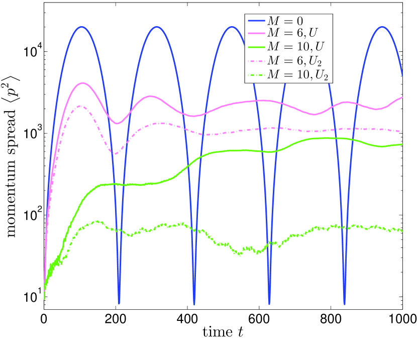
Figure 1: (Color online) Momentum spread $\left\langle p^{2}\right\rangle$ as a function of number of kicks (time $t$). Solid lines represent results generated by the Floquet operator ${U}$ defined in Eq. (3), with the initial state given by spin-up and a Gaussian wavepacket $\sim\exp(-p^{2}/2\sigma_{p}^{2})$. The dot-dashed lines represents the results generated by a spinless Floquet operator ${U}_{2}$ defined in Eq. (5), with the initial wavepacket given by the Gaussian $\sim\exp(-p^{2}/2\sigma_{p}^{2})$. In both cases, $\sigma_{p}=4$, irrational $\alpha=1/3+0.01/2\pi$, $K=0.8$, $q=3$ and $M$ takes values of 0, 6 and 10. (Results of ${U}$ and ${U}_{2}$ with $M=0$ are identical.) $\left\langle p^{2}\right\rangle$ is seen to be strongly localized in all the examined examples. Here and in all other figures, all plotted quantities are in dimensionless units.

With the same set of system parameters, the mean momentum spread under the evolution of the Floquet operator ${U}$ is similar to that under the evolution of its spinless version ${U}_{2}$. This confirms that the common on-site phase accumulation function $\Phi_{p}$ has captured the main features of dynamical localization. It is also interesting to comment on the differences between these two cases. That is, $\left\langle p^{2}\right\rangle$ associated with ${U}$ is always larger than that associated with ${U}_{2}$. As such, the spin degree of freedom is seen to slightly weaken dynamical localization. This is somewhat expected. Indeed, the spin degree of freedom introduces two channels for the dynamics and a multi-channel Anderson model does increase the localization length Mello1988 . We note in passing that the spin degree of freedom can even cause Anderson transition in two-dimensional disordered systems Evangelou1987 ; Sheng1996 . Certainly, as $M$ increases, this spin effect should decrease because it becomes more costly in energy for the two spin channels to interact.

Finally, we mention the benchmark result in Fig. 1 for the $M=0$ case that represents the Maryland model. The perfect revival of $\left\langle p^{2}\right\rangle$ was predicted by Berry Berry1984 . Using our system parameters depicted in the caption of Fig. 1, Berry’s result gives $\left\langle p^{2}\right\rangle(t)\sim\sin^{2}0.015t/\sin^{2}0.015$ and our simulation agrees with this.

III.2 Superballistic transport for rational $\alpha$ and on-resonance potential

As we already discussed in the previous subsection, for large momentum values, the effect of a nonzero mass term $M$ will diminish and effectively the Maryland model will re-emerge. So if we were not to choose an on-resonance potential, then in regimes of large momentum quantum revivals should occur for rational $\alpha$, which is not of interest here. In addition, we also observed that for an off-resonance kicking potential and for rational $\alpha$, a non-zero $M$ further suppresses the already bounded momentum spread. With these understandings, it is clear that we should step into the interesting situation where $\alpha=r/s$ is rational and the kicking potential $K\cos(q\theta)$ is on resonance, i.e, $q=ns$. For convenience we choose $q=s$. Reference Matrasulov2005 computationally investigated exactly the same situation, but it was argued therein that the phase factor $\Phi_{p}$ as a pseudo-random function of momentum should suffice to localize the momentum spread. As we show below, both qualitatively and quantitatively, this claim is correct only for low momentum values, and overall a much richer transport behavior can be found.

Let us start with the Maryland model for which $M=0$. Then the momentum space is translational invariant with period $s$. As such, states will in general spread ballistically (the off-resonance case is an exception). In our case, $M\neq 0$ and within each period, the on-site phase $\Phi_{p}$ acquired by the system becomes a quasi-random function of $p$, thus dynamical Anderson localization or suppression of momentum spread is expected. However, as momentum increases, the nonzero $M^{2}$ term in $\Phi_{p}=\exp\left(\pm i[\sqrt{(2\pi\alpha p)^{2}+M^{2}}]\right)$ becomes less important as compared with $(2\pi\alpha p)^{2}$. For very large momentum, the $M^{2}$ term represents a very weak perturbation and hence the dynamics should resemble that of the Maryland model.

The above qualitative analysis makes it clear that the overall dynamics depends on many factors. On a sublattice representing low momentum values from $-p_{c}$ to $+p_{c}$, dynamical localization takes place and the system is effectively in a disordered regime. On a sublattice representing higher momentum values, ballistic transport is expected and the system is effectively in a periodic regime. Whether or not a state is localized or delocalized now depends on where it is initially located, and on the size of the disordered regime as compared with the localization length. For example, if an initial state is localized at the center of the disordered regime and if the localization length is much shorter than the disordered region, then the system may be trapped there for an extremely long time. On the other hand, if the initial state is already located close to the high-momentum sublattice (closeness is with respect to the localization length), then as the kicking field induces population transfer between the disordered sublattice and the periodic sublattice, the system will be quickly delocalized. In this sense, our model, through its natural dispersion relation, realizes a lattice junction analogous to that considered in Refs. Hufnagel2001 ; Zhenjun2012 . Certainly, in our model here there is no sharp transition between the two qualitatively different sublattices, but the critical momentum value is expected to scale with $M/(2\pi\alpha)$.

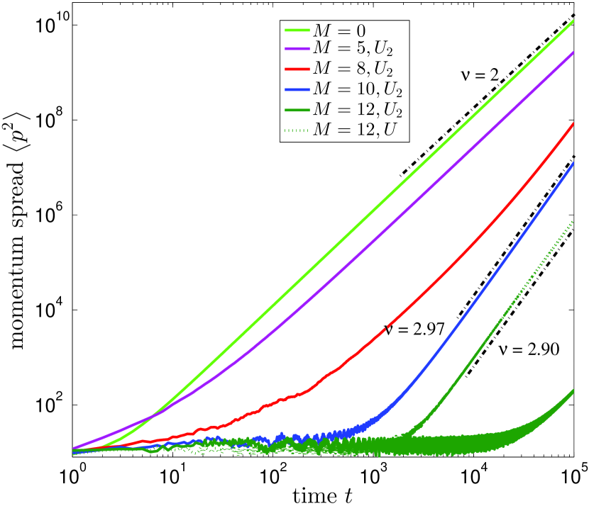
Figure 2: (Color online) Ensemble averaged momentum spread $\left\langle p^{2}\right\rangle$ vs time, for $M=0$, $M=5$, $M=8$, $M=10$ and $M=12$ (from top to bottom). Results with $M=5$, $M=8$, $M=10$ are for the spinless Floquet operator ${U}_{2}$ defined in Eq. (5). For $M=12$, results for both ${U}$ (the one fitted by a power-law with $\nu=2.90$) and ${U}_{2}$ (the most localized case) are plotted. (Result with $M=0$ is applicable to both ${U}$ and ${U}_{2}$.) Other system parameters are the same as in Fig. 1, except for $\alpha=1/3$. The two dashed straight lines represent a power-law fitting $\left\langle p^{2}\right\rangle\propto t^{\nu}$ (for a certain time window) with $\nu=2.90$ or $\nu=2.97$, indicating quantum superballistic transport with an exponent close to $\nu=3$.

Representative results from our numerical experiments are presented in Fig. 2. There it is seen that as $M$ increases, an initial state localized at the center of the disordered sublattice will be trapped for a longer period. This is consistent with our understanding that an increasing $M$ leads to a longer disordered sublattice as well as a shorter localization length. Other numerical results (not shown) show that the values of $\alpha$, the kicking strength $K$, and the potential parameter $q$ can all affect the duration during which an initial state is trapped in the disordered regime.

Two of the computational examples shown in Fig. 2 also display quantum superballistic transport, i.e. $\left\langle p^{2}\right\rangle\propto t^{\nu}$ with $\nu>2$, where $t$ is the number of kicks. This can now be explained using the idea from Ref. Hufnagel2001 . In particular, assuming that the length of the disordered momentum sublattice is larger than the corresponding localization length, then the disordered regime serves as a source to provide slow probability leakage into a periodic regime at an almost constant rate. Then we have

$$\left\langle p^{2}\right\rangle(t)\approx B+aCt^{2}+a\int^{t}_{0}{R(t^{\prime})(t-t^{\prime})^{2}\mathrm{d}t^{\prime}}.$$ (7)

Here $R(t)$ is the probability leaking rate from the disordered sublattice to the periodic sublattice, $B$ represents the contribution from the disordered regime, which is almost constant and can be neglected. $C$ represents the probability of the initial state already placed in the periodic regime, which is 0 due to our choice of the initial state located at the center of the disordered regime. $a$ characterizes the ballistic transport coefficient, which depends on many system parameters. If we approximate $R(t)$ by a constant $\Gamma$, then from Eq. (7) we approximately have

$$\left\langle p^{2}\right\rangle(t)\propto a\Gamma t^{3}.$$ (8)

As reflected by the two cases shown in Fig. 2, namely, the case of $M=12$ for the full Floquet operator ${U}$ and the case of $M=10$ for the spinless Floquet operator ${U}_{2}$ defined in Eq. (5), $\left\langle p^{2}\right\rangle\propto t^{\nu}$, with $\nu\approx 2.90$ or $\nu\approx 2.97$, for a very long time scale and covering a huge range of $\left\langle p^{2}\right\rangle$ (note the logarithmic scales used in the plot). These two superballistic exponents are very close to $\nu=3$, in agreement with the above theory. For the same two cases, we have set $p_{c}\approx 100M/(2\pi\alpha)$ and record the probabilities inside $[-p_{c},p_{c}]$ as a function of time. This probability indeed decreases linearly with time. This further confirms the physical mechanism behind the quantum superballistic transport seen here. The case shown in Fig. 2 with $M=5$ displays ballistic transport as the case of $M=0$. This is so because for a small value of $M$ the initial state quickly experiences ballistic transport on the clean sublattice. For the intermediate case $M=8$, the momentum spread does not show any clear power-law dependence. In this transitional case, the localization length and the size of disordered lattice are comparable and hence the leakage from the disordered sublattice to the periodic sublattice occurs no longer at an almost constant rate. We stress that the shown cases represent but a few examples. Many similar results of quantum superballistic transport are obtained for both the full Floquet operator ${U}$ involving two spin channels and for the spinless Floquet operator ${U}_{2}$.

Though the quantum superballistic transport here is explained in the same manner as in Ref.  Hufnagel2001 , we stress that the effective two-sublattice configuration is not artificially designed. Rather, it emerges as a natural consequence of the relativistic dispersion relation with a nonzero mass.

IV Classical dynamics

IV.1 Classical phase space structure

In this subsection we will study the classical relativistic KR described by the Hamiltonian in Eq. (6). To that end, it is necessary to examine the phase space structure, which can be generated from the relativistic standard map Chernikov1989 ; Nomura1992 . In particular, the states right after the $N$-th and $N+1$-st kick are connected by the map

$$\begin{split}\theta_{N+1}&=\frac{v^{2}p_{N}}{\sqrt{v^{2}p_{N}^{2}+M^{2}}}+\theta_{N}\ \ (\text{mod }2\pi/q),\\ p_{N+1}&=qK\sin(q\theta_{N+1})+p_{N}.\end{split}$$ (9)

In the quantum case, either an irrational $\alpha$ or a non-resonant kicking potential causes localization. Considering quantum-classical correspondence, this suggests bounded (i.e., localized in momentum) invariant curves in the phase space. Results in Fig. 3(b)-(d) support this view.

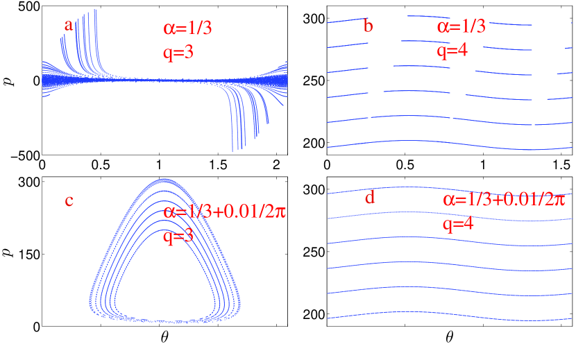
Figure 3: (Color online) Phase space structure of $H_{C}$ defined in Eq. (6), for four different situations, namely, (a) rational $\alpha$ and on-resonance kicking potential, (b) irrational $\alpha$ with off-resonance kicking potential, (c) irrational $\alpha$ with an almost on-resonance kicking potential; and (d) irrational $\alpha$ with an off-resonance kicking potential. $M=10$ and $K=1.6$. The phase space invariant curves are seen to be unbounded in momentum in panel (a), but bounded in panels (b)-(d).

To understand the phase space structure, we first recall the Maryland model Berry1984 , which can approximately describe the dynamics for sufficiently large momentum values. That is, if $p$ is large, then we again neglect the $M$ term in the Hamiltonian. Then the mapping in Eq. (9) (after dropping the $M$ term) reduces to the mapping associated with the Maryland model. For the Maryland model, the following equations hold for either an irrational $\alpha$ or a non-resonant kicking potential:

$$\begin{split}\theta_{N}&=Nv+\theta_{0},\\ p_{N}&=\frac{1}{2}\csc\frac{qv}{2}\left(\cos(\frac{qv}{2}+q\theta_{0})-\cos\left[(N+\frac{1}{2})qv+q\theta_{0}\right]\right)\\ &\quad+p_{0},\end{split}$$ (10)

where as introduced before, $v=2\pi\alpha$. Clearly then, for an irrational $\alpha$, the term $Nv$ can densely cover the entire $\theta$ domain $[0,2\pi]$. As such, as $N$ increases, the values of $(\theta_{N},p_{N})$ fill a complete sine curve in the phase space. On the other hand, if $\alpha$ is rational, $q\alpha$ becomes a fraction under the assumed off-resonance condition, then $\theta_{N}$ can only take discrete points in $[0,2\pi]$ such that $p_{N}$ also takes a few isolated values Berry1984 .

These observations for the Maryland model can be used to directly explain the panel (d) in Fig. 3. For panel (b) where $\alpha$ is rational but the kicking potential is off resonance, a nonzero $M$ also causes the dynamics to densely fill the entire $\theta$ domain, which constitutes an interesting difference from the Maryland model. However, as expected, after the same number of iterations, regimes with low momentum values can generate a complete phase invariant curve faster, and regimes with high momentum values may still have holes to be filled in. As to panel (c) where the product of $\alpha q$ is close to an integer, the oscillation amplitude in momentum get larger as the factor $\csc\frac{qv}{2}$ in the map in Eq. (10) can be a large number. Putting all these cases together, it is seen that in the three situations represented by panels (b)-(d) of Fig. 3, KAM invariant curves localized in momentum are the main characteristic of the classical phase space.

So now we are left with the last situation in which $\alpha$ is rational and the kicking potential is on resonance. The associated phase space structure is presented in panel (a) of Fig. 3 and in Fig. 4. The phase space structure is remarkably complicated and interesting. To investigate this in detail, we divide the phase space into four regimes, namely regimes I, II, III and IV for increasing absolute values of momentum.

Let us take one example to look into the special phase space structure. As seen in Fig. 4 for $K=0.8$, $M=10$, the four regimes have qualitatively different behavior. In regime I where $p$ is small, local KAM curves dominate. As $p$ increases, the feature of the phase space become chaotic in regime II. This is followed by global KAM curves in regime III. These global KAM curves are localized in momentum and bound the chaotic sea seen in regime II. Finally, in regime IV for quite large momentum, ballistic curves, which become more and more parallel to the momentum axis, are seen. These curves are called ballistic curves because once a trajectory lands on such a structure its momentum variance will evolve ballistically.

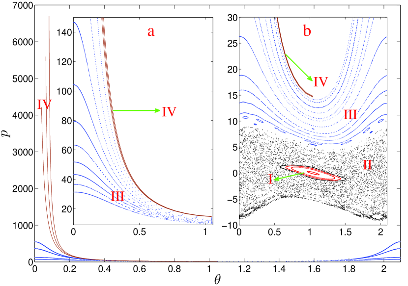
Figure 4: (Color online) Detailed phase space structure for a situation similar to panel (a) in Fig. 3. Here system parameters are given by $K=0.8$, $M=10$, $\alpha=1/3$, and $q=3$. Panel (a) depicts regimes with large momentum values, and panel (b) depicts regimes with low momentum values. Curves in regime I are local KAM curves, KAM curves in regime III are global curves and hence localize momentum. The black dots regime in II are generated by a single initial condition and indicate a chaotic sea. Curves in regimes IV that are almost parallel to the momentum axis are ballistic structures.

The four regimes identified above may not always appear together. Their presence and borders are determined by $M$ and $K$. To shed some light on this, one may consider $H_{C}$, in the two opposite limits, i.e., “non-relativistic” $vp\ll M$ limit and “ultra-relativistic” limit $vp\gg M$. In the first limit, $H_{C}$ becomes

$$H_{S}=M+\frac{1}{2}\frac{v^{2}p^{2}}{M}+K\cos q\theta\sum_{n=-\infty}^{\infty}{\delta(t-n)},$$ (11)

and in the second limit, $H_{C}$ assumes

$$H_{L}=v|p|+K\cos q\theta\sum_{n=-\infty}^{\infty}{\delta(t-n)}.$$ (12)

Regimes I and II can be understood via $H_{S}$, while regime IV can be well understood by $H_{L}$. In particular, $H_{S}$ is the conventional kicked rotor, which makes the regular-to-chaotic transition as $K$ increases CasatiBook1995 . $H_{L}$ is much similar to the Hamiltonian of the Maryland model, which is known to produce ballistic trajectories in the momentum space Berry1984 . Indeed, it can be shown that the asymptotic (in the large $p$ limit) form of the ballistic trajectories are described by $\theta=\text{constant}$, and they are hence completely parallel to the momentum axis.

As is found from our computational studies, an increase in $K$ may destroy the KAM curves in regimes I and III, and then turns them to a (possibly transient) chaotic sea as well. An increase in $M$ will generate more KAM curves in the phase space. The complexity of the phase space perhaps deserves more careful studies. For our purpose here, we emphasize that for a sufficiently large $K$, the phase space is mainly composed of a seemingly chaotic sea and ballistic trajectories. It is however challenging to identify a clear boundary between trajectories eventually landing on the ballistic structure and those always doing random motion. To appreciate this complexity, in Fig. 5 we illustrate that once global curves are all broken, how an individual trajectory might eventually land on the ballistic structure after transient, but a long period of, “chaotic” motion. The whole process is like the following: after the system has wandered in the transient chaotic sea [see panel (b)] for a long time, the system finally reaches $L_{1}$ and keeps moving to the left. Then it reaches $L^{{}^{\prime}}_{1}$ and continues to move towards the left. It then passes the central transient “chaotic sea”. Later the system has a chance to arrive $L_{2}$, followed by $L^{{}^{\prime}}_{2}$. The system eventually reach a ballistic curve $L_{3}$ and then keeps moving up in the momentum space. In brief, it takes 3 stages for a trajectory launched from the regime illustrated in panel (b) of Fig. 5 to finally turn to ballistic motion. First, it wanders highly randomly in a transient chaotic sea. Second, it moves alternatively along some smooth curves [such as those shown in panel (a) and panel (c) in Fig. 5], between which the system returns to the transient chaotic sea, but with the overall tendency towards curves of large momentum values. Lastly, the system evolves on a simple ballistic structure.

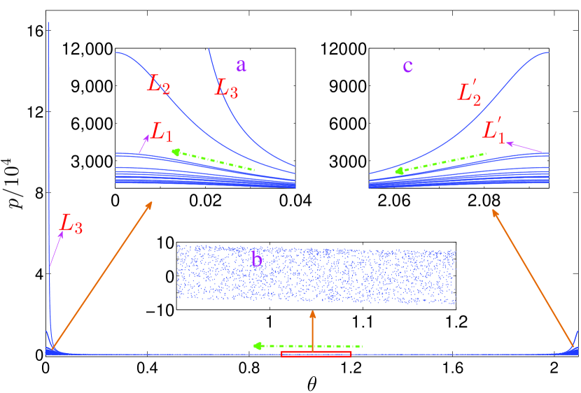
Figure 5: (Color online) Evolution of a single trajectory from $(\theta_{0},p_{0})=(0,0.7)$. The total evolution time is $2\times 10^{6}$, by which time this trajectory becomes clearly ballistic. The whole process is remarkably complicated. Panels (a) (b) and (c) zoom in some small portions of the shown phase space, with the momentum values in the middle-$\theta$ regime seen to be highly localized. Green dash-dotted arrow shows the moving direction of the trajectory along the “curves” traced by the trajectory. These curves shown here emerges after $t\approx 7.6\times 10^{5}$, and similar curves developed in earlier time with smaller $p$ values. Note that these curves are not KAM invariant curves as the system will eventually leave them. We define the motion along these curves as “transient chaotic motion”.

IV.2 Classical superballistic transport

In our simulations, we always choose $10^{5}$ phase space points randomly sampled from the following Gaussian distribution

$$f(p,\theta)=\frac{1}{2\pi\sigma_{p}\sigma_{\theta}}\text{exp}(-\frac{p^{2}}{2\sigma_{p}^{2}})\text{exp}(-\frac{\theta^{2}}{2\sigma_{\theta}^{2}}).$$ (13)

Note that this Gaussian distribution is analogous to the initial Gaussian wavepacket we used in our quantum dynamics calculations. We then evolve this ensemble of classical trajectories according to the relativistic KR map described by Eq. (9) and examine the ensemble averaged $\left\langle p^{2}\right\rangle$ as a function of $t$, i.e., the number of iterations. Interestingly, the time dependence of $\left\langle p^{2}\right\rangle$ is rich, and if we fit $\left\langle p^{2}\right\rangle$ by the power-law $\sim t^{\nu}$ for appropriate time windows, the exponent $\nu$ can be larger than 2. In fact, sometimes $\nu$ can be even larger than three or even four. Some examples are shown in Fig. 6. In one case, the superballistic transport exponent is found to be as large as $\nu=4.2$, for a time window from $t=10^{6}$ to $t=3\times 10^{6}$. On the one hand this confirms that the classical dynamics may display superballistic transport, on the other hand it is necessary to better understand the underlying mechanism. By exploring many parameter choices, it is found that breaking the global KAM curves with an increasing ratio $K/M$ is a necessary condition. This is already a clear difference from quantum superballistic transport. For example, for the results shown in Fig. 2, $v=2\pi/3$, $q=3$, $M=10$, quantum superballistic transport occurs already for $K=0.8$, but in the classical case shown in Fig. 6, superballistic transport is observed only when $K$ exceeds 1.4. Thus, in the quantum case, a global KAM invariant curve does not forbid the population leakage from the classically chaotic regime to the ballistic regime, an indication of quantum tunneling.

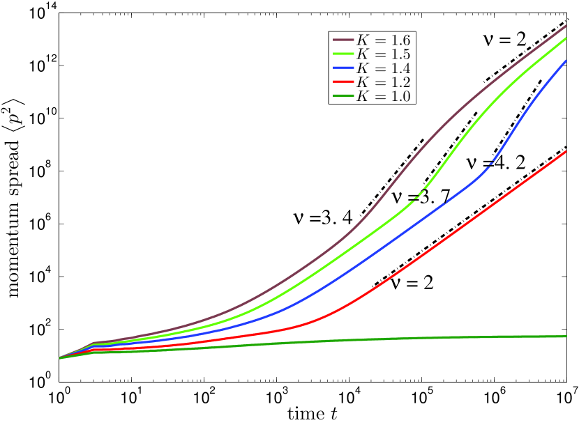
Figure 6: (Color online) Ensemble averaged classical momentum spread $\left\langle p^{2}\right\rangle$ vs time (the number of kicks). The initial conditions are sampled from a Gaussian distribution described by Eq. (13) with $\sigma_{p}=2\sqrt{2}$ and $\sigma_{\theta}=1/\sigma_{p}$, so that the initial phase space distribution is analogous to the quantum initial state used in Fig. 2. Here $v=2\pi/3$, $q=3$, $M=10$, and from top to bottom, $K=1.6,1.5,1.4,1.2$, and $1.0$. Note that with other system parameters being the same, quantum superballistic transport already occurs for $K=0.8$ (see Fig. 2). Here the classical superballistic transport emerges until $K$ reaches 1.4.

To further understand the numerical results, we find it necessary to also account for normal diffusion as the trajectories seek to land on ballistic trajectories from the chaotic sea. The associated normal diffusion rate is assumed to be $D_{0}$. We further assume that the leakage rate from the chaotic sea to the ballistic structure is given by $R(t)$. Then analogous to Eq. (7), we expect to have

$$\left\langle p^{2}\right\rangle(t)\approx B+Dt+aCt^{2}+a\int_{0}^{t}R(t^{\prime})(t-t^{\prime})^{2}\mathrm{d}t^{\prime},$$ (14)

where $B=\rho_{0}\overline{p^{2}_{0}}$, with $\rho_{0}$ being the fraction of trajectories confined in some local stable islands in Regime I and $\overline{p^{2}_{0}}$ being their average momentum spread; $D=\rho_{1}D_{0}$, with $\rho_{1}$ representing the fraction of trajectories undergoing normal diffusion, with $D_{0}$ being the associated diffusion constant; $C=\rho_{2}$ is the faction of trajectories initially placed on ballistic structures, with $a$ being the diffusion coefficient. Note that, unlike in the quantum case, at this point we do not first assume a constant probability leakage rate because, as seen below, the leakage involves different behavior at different time windows, and so $R(t)$ can be rather complicated. Indeed, as seen from Fig. 5, once the global KAM curves are destroyed, the escape from a (transient) chaotic sea to a ballistic structure is extremely complicated: the boundary between them is hard to identify and different initial conditions sampled from an initial Gaussian ensemble may need drastically different times to reach a ballistic structure.

The coexistence of normal diffusion, ballistic transport, and the potentially complicated leakage rate $R(t)$ makes the time dependence of $\left\langle p^{2}\right\rangle(t)$ even more interesting than the quantum case. Let us roughly define a regime $[-P_{0},P_{0}]$ in the phase space, where trajectories are not doing ballistic motion. In connection with our observations made from Fig. 5, we choose $P_{0}=500$. Let $P_{c}(t)$ be the occupation probability of this regime and $P_{u}(t)=1-P_{c}(t)$ be the occupation probability on ballistic structures. Then $R(t)=-\frac{\mathrm{d}P_{c}(t)}{\mathrm{d}t}$. $P_{c}(t)$ is plotted in Fig. 7 on either linear or logarithmic scales, for different time windows, for the value $K=1.4$ already studied in Fig. 6. The right inset of Fig. 7 indicates that initially most trajectories are trapped in the regime $[-P_{0},P_{0}]$, until $t=t_{1}\approx 5\times 10^{4}$. Then $P_{c}(t)$ starts to decrease more appreciably, with a time dependence not easy to fit [see the first part of the curve in panel (c)]. After $t=t_{2}\approx 5\times 10^{5}$ kicks however, the relation between $P_{c}(t)$ and $t$ becomes much more evident, i.e. $\ln P_{c}(t)\propto-\Gamma t$, which indicates an exponential decay. The emergence of an exponential decay suggests that the ensemble has reached a certain steady configuration, as the escape probability now becomes proportional to the occupation probability itself. As also shown by the bottom inset and by the main figure of Fig. 7, the coefficient $\Gamma$ slightly changes with time. Expanding such an exponential decay to the first order, this escape would amount to an almost constant leakage rate of jumping onto phase space ballistic structures. As a result, one would naively expect, like our analysis in the quantum part, a superballistic transport case with $\nu=3$. This prediction is certainly oversimplified as compared with our actual results shown in Fig. 6.

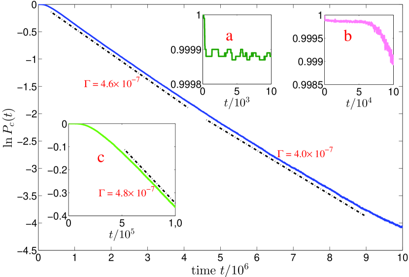
Figure 7: (Color online) Results of $\ln P_{c}(t)$ vs time, where $P_{c}$ defined in the text represents the occupation probability in a non-ballistic regime. For the two insets (a) and (b), $P_{c}(t)$ vs time is plotted for two early stages, where it can be seen that initially most trajectories are trapped in the initial non-ballistic regime for $t<t_{1}\approx 5\times 10^{4}$. Then $P_{c}(t)$ starts to decrease appreciably in a nonlinear fashion. The inset (c) shows that the time dependence of $\ln P_{c}(t)$ is highly nonlinear before $t=t_{2}$. However, after $t_{2}\approx 5\times 10^{5}$, $\ln P_{c}(t)$ and $t$ display a linear relation. The system parameters are the same as the case of $K=1.4$ in Fig. 6.

To better digest the results shown in Fig. 6, we again focus on the case $K=1.4$ in connection with the time dependence of $P_{c}(t)$ in Fig. 7. In the very beginning, $P_{c}(t)$ remains almost a constant until $t_{1}\approx 5\times 10^{4}$ kicks, so for this time period $R(t)$ is essentially zero. Therefore initially only the first three terms in Eq. (14) are non-zero, suggesting that the diffusion exponent of $\left\langle p^{2}\right\rangle$ should be less than two. This explains the actual numerical result during the early stage. The plotted curve in Fig. 6 at early times also has an increasing slope. This can be explained as follows. During the early stage, we have $B>D>aC$. When $t>B/D$, the $Dt$ term starts to dominate so $\left\langle p^{2}\right\rangle$ is close to normal diffusion. Similarly, when $t>D/(aC)\approx 10^{3}$, the $aCt^{2}$ term exceeds the first two, so we have a behavior close to ballistic transport for a quite long period until $t=t_{2}\approx 5\times 10^{5}$. On the other hand, from Fig. 7, it is observed that since as early as $t=t_{1}\approx 5\times 10^{4}$, $R(t)$ is already non-zero. So the leakage to the ballistic regime is building up long before an exponential leakage is observed at $t>t_{2}$. This early-stage leakage to the ballistic regime starts to affect the time dependence of $\left\langle p^{2}\right\rangle$ only until $t\approx 10^{6}$. We conjecture that this is the reason why in Fig. 6 a simple relation $\left\langle p^{2}\right\rangle(t)\sim t^{3}$ is not observed. In addition, the lack of such a simple superballistic behavior with $\nu=3$ is also consistent with the apparent nonlinear time dependence shown in panel (c) of Fig. 7 before $t=t_{2}$.

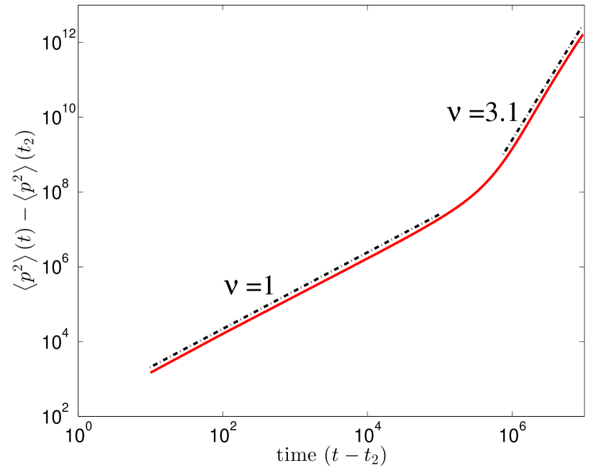
Figure 8: (Color online) $[\left\langle p^{2}\right\rangle(t)-\left\langle p^{2}\right\rangle(t_{2})]$ vs $(t-t_{2})$, an analysis motivated by a reset of the start time at $t=t_{2}$ (see the text for the details). The result here mainly displays a normal diffusion stage and a superballistic transport stage with an exponent close to $\nu=3$. The computational example presented here is the same one in Fig. 7 with $K=1.4$. The dashes lines represent power-law fitting.

To confirm our qualitative analysis above, we now redefine the start time as the point when an exponential decay of $P_{c}(t)$ can be clearly identified. Again using the computational example shown in Fig. 7, we now use $t_{2}\approx 5\times 10^{5}$ as the start time to count change in the momentum spread. That is, we now examine $\left[\left\langle p^{2}\right\rangle(t)-\left\langle p^{2}\right\rangle(t_{2})\right]$. Because at $t_{2}$, the population inside the regime $[-P_{0},P_{0}]$ is about 0.88, we have $P_{c}(t)=0.88\exp[-\Gamma(t-t_{2})]$. Then we have

$$\begin{split}\left[\left\langle p^{2}\right\rangle(t)-\left\langle p^{2}\right\rangle(t_{2})\right]&\approx 0.88\ D_{0}e^{-\Gamma(t-t_{2})}(t-t_{2})\\ &\quad+0.12\ a(t-t_{2})^{2}\\ &\quad+a\int^{t}_{t_{2}}{R(t^{\prime})(t-t^{\prime})^{2}\mathrm{d}t^{\prime}},\end{split}$$ (15)

where the first term account for the normal diffusion as the trajectories diffuse from a chaotic sea to eventually land on a ballistic structure, the second term describes the ballistic transport for those trajectories already outside the regime $[-P_{0},P_{0}]$ at the start time $t_{2}$, and the last term describes the impact on the transport dynamics due to the population leakage from the regime $[-P_{0},P_{0}]$, with

$$R(t) = -\frac{dP_{c}}{dt}$$ (16)

$$= 0.88\ \Gamma\exp[-\Gamma(t-t_{2}]\approx 0.88\ \Gamma.$$

Equation (15) thus suggests that once we reset the start time at $t_{2}$, there should be a normal diffusion stage, a transition stage due to the second term, followed by a superballistic transport period, i.e., $[\left\langle p^{2}\right\rangle(t)-\left\langle p^{2}\right\rangle(t_{2})]\sim(t-t_{2})^{3}$. In Fig. 8 we present a numerical log-log plot of $\left[\left\langle p^{2}\right\rangle(t)-\left\langle p^{2}\right\rangle(t_{2})\right]$ vs $(t-t_{2})$, in very good agreement with our analysis. As a final note, the classical superballistic transport shown in Fig. 8 with the diffusion exponent $\nu\approx 3.1$ lasts very long, but this behavior cannot last forever. In the end, almost all trajectories from the initial ensemble will end up on ballistic structures and then purely ballistic transport will take over.

Returning to an early study Matrasulov2005 of the classical relativistic KR under the resonance condition, we have to disagree with some of their statements; from our results we conclude that classical superballistic transport was not observed there because the investigation time scale there was too short.

V Conclusions

In this work, we show that both quantum and classical superballistic transport can occur in a simple periodically driven system, namely, a relativistic kicked-rotor system with a nonzero mass term. To our knowledge, this appealing scenario has not been discussed before. Compared with previous lattice-junction models for quantum superballistic transport, the superballistic transport in our model occurs in momentum space as a consequence of a natural divide imposed by the relativistic dispersion: regions with low momentum effectively have a quadratic (bare) dispersion relation (hence effectively a quasi-random on-site potential) and regions of high momentum effectively have a linear (bare) dispersion relation (hence effectively a quasiperiodic potential).

Remarkably, though found in the same dynamical system, the quantum superballistic and classical superballistic transport we have analyzed are observed in much different parameter regimes. Indeed, in the quantum case, the mechanism lies in the leakage of the quantum state from a regime of dynamical localization to a regime of ballistic transport. This leakage can occur even when the underlying classical limit has global KAM invariant curves separating the two regimes. In the classical case, it is necessary to break the global KAM curves first to allow for leakage from a chaotic sea to ballistic trajectories. As a side result, we find that this kind of leakage in the classical dynamics is unexpectedly complicated and further studies can be motivated. For example, strictly speaking, the random patterns shown in the panel (b) of Fig. 5 do not represent chaos (chaos is defined as a positive Lyapunov exponent in the asymptotic long-time limit, but this trajectory will eventually become ballistic and hence has a zero Lyapunov exponent). The detailed characteristics of this type of irregular trajectory eventually becoming a regular ballistic one deserve more attention. The issue of quantum-classical correspondence concerning this type of trajectories is also of considerable interest for future studies.

The classical relativistic kicked rotor model may be realized by considering relativistic electrons moving in the field generated by a special electrostatic wavepacket Chernikov1989 . On the quantum side, a spinless version of the relativistic kicked rotor may be also realized by considering a kicked tight-binding lattice whose on-site potential can be determined by the relativistic dispersion relation  Gong2007 ; Monteiro . However, due to the large time scales involved, a direct observation of our numerical results reported here is unlikely. As such it should be interesting enough to explore the system more to identify other signatures of superballistic transport at shorter time scales.

References

- (1) B. D. Hughes, Random Walks and Random Environments (Clarendon Press, Oxford, 1995).
- (2) Y. He, S. Burov, R. Metzler, and E. Barkai, Phys. Rev. Lett. 101, 058101 (2008).
- (3) R. Metzler and J. Klafter, Phys. Rep. 339, 1 (2000).
- (4) J. P. Bouchaud and A. Georges, Phys. Rep. 195, 127 (1990).
- (5) B. I. Henry, T.A.M. Langlands, and P. Straka, in Complex Physical, Biophysical and Econophysical Systems, World Scientific Lecture Notes in Complex Systems, edited by R. L. Dewar and F. Detering (World Scientific, Singapore, 2010), Vol. 9.
- (6) J. Wang, I. Guarneri, G. Casati, and J. B. Gong, Phys. Rev. Lett. 107, 234104 (2011); H. L. Wang, J. Wang, I. Guarneri, G. Casati, and J. B. Gong, Phys. Rev. E 88, 052919 (2013).
- (7) S. Abe and H. Hiramoto, Phys. Rev. A 36, 5349 (1987); H. Hiramoto and S. Abe, J. Phys. Soc. Jpn. 57, 230 (1988); 57, 1365 (1988).
- (8) F. Piéchon, Phys. Rev. Lett. 76, 4372 (1996).
- (9) R. Ketzmerick, K. Kruse, S. Kraut, and T. Geisel, Phys. Rev. Lett. 79, 1959 (1997).
- (10) K. Lü and J.-D. Bao, Phys. Rev. E 76, 061119 (2007).
- (11) P. Siegle, I. Goychuk, P. Talkner, and P. Hänggi, Phys. Rev. E 81, 011136 (2010); P. Siegle, I. Goychuk, and P. Hänggi, Phys. Rev. Lett. 105, 100602 (2010); P. Siegle, I. Goychuk, and P. Hänggi, Europhys. Lett. 93, 20002 (2011).
- (12) L. Levi, Y. Krivolapov, S. Fishman and M. Segev, Nat. Phys. 8, 912 (2012).
- (13) L. Hufnagel, R. Ketzmerick, T. Kottos, and T. Geisel, Phys. Rev. E 64, 012301 (2001).
- (14) Z. J. Zhang, P. Q. Tong, J. B. Gong, and B. W. Li, Phys. Rev. Lett. 108, 070603 (2012).
- (15) S. Stützer, T. Kottos, A. Tünnermann, S. Nolte, D. N. Christodoulides, and A. Szameit, Opt. Lett. 38, 4675 (2013).
- (16) A. A. Chernikov, T. Tեl, G. Vattay, and G. M. Zaslavsky, Phys. Rev. A 40, 4072 (1989).
- (17) D. U. Matrasulov, G. M. Milibaeva, U. R. Salomov, and B. Sundaram, Phys. Rev. E 72, 016213 (2005).
- (18) G. Casati and B. V. Chirikov, Quantum Chaos: Between Order and Disorder (Cambridge University Press, New York, 1995).
- (19) D. R. Grempel, S. Fishman, and R. E. Prange, Phys. Rev. Lett. 49, 833 (1982).
- (20) R. E. Prange, D. R. Grempel, and S. Fishman, Phys. Rev. B 29, 6500 (1982).
- (21) M. V. Berry, Physica D 10, 369 (1984).
- (22) B. Simon, Annals of Physics 159, 157 (1985).
- (23) Y. Nomura, Y. H. Ichikawa, and W. Horton, Phys. Rev. A 45, 1103 (1992).
- (24) S. Fishman, D. R. Grempel, and R. E. Prange, Phys. Rev. Lett. 49, 509 (1982).
- (25) P. Mello, P. Pereyra, and N. Kumar, Ann. Phys. 181, 290 (1988).
- (26) S. N. Evangelou and T. Ziman, Journal of Physics C: Solid State Physics 20, L235 (1987).
- (27) D. N. Sheng and Z. Y. Weng, Phys. Rev. B 54, R11070 (1996).
- (28) J. B. Gong and J. Wang, Phys. Rev. E 76, 036217 (2007).
- (29) T. Boness, S. Bose, and T. S. Monteiro, Phys. Rev. Lett. 96 , 187201 (2006).