Eccentricity distributions in nucleus-nucleus collisions

Abstract

We propose a new parametrization of the distribution of the initial eccentricity in a nucleus-nucleus collision at a fixed centrality, which we name the Elliptic Power distribution. It is a two-parameter distribution, where one of the parameters corresponds to the intrinsic eccentricity, while the other parameter controls the magnitude of eccentricity fluctuations. Unlike the previously used Bessel-Gaussian distribution, which becomes worse for more peripheral collisions, the new Elliptic Power distribution fits several Monte Carlo models of the initial state for all centralities.

I Introduction

Elliptic flow, $v_{2}$, is a crucial observable of heavy-ion collisions: the large magnitude of $v_{2}$ at RHIC Ackermann:2000tr ; Adler:2003kt and LHC Aamodt:2010pa ; ATLAS:2011ah ; Chatrchyan:2012ta provides the strongest evidence that a low-viscosity fluid is formed in these collisions Romatschke:2007mq ; Luzum:2008cw . Elliptic flow is determined to a good approximation by linear response to the initial eccentricity $\varepsilon_{2}$, which quantifies the spatial azimuthal anisotropy of the fireball created right after the collision Alver:2006wh . This initial eccentricity comes from two effects: first, the overlap area between the colliding nuclei has the shape of an almond in non-central collisions, where the smaller dimension of the almond is parallel to the reaction plane. This results in an eccentricity which becomes larger as impact parameter increases, and whose magnitude is model dependent Hirano:2005xf ; Lappi:2006xc . Second, even in central collisions, there is a sizable eccentricity due to quantum fluctuations in wave functions of incoming nuclei Miller:2003kd ; Alver:2006wh , and to the probabilistic nature of energy deposition in nucleon-nucleon collisions. The magnitude of these eccentricity fluctuations is again a model-dependent issue, which involves the dynamics of the collision at early times Miller:2007ri ; Flensburg:2011wx ; Dumitru:2012yr ; Schenke:2012hg . The goal of this paper is to show that the distribution of the initial eccentricity is to some extent independent of model details. More precisely, it can be written to a good approximation as a universal function of two parameters, where one of the parameters corresponds to the reaction plane eccentricity, and the other parameter characterizes the magnitude of fluctuations. Information on the initial state is thus encoded in two numbers.

The initial eccentricity $\varepsilon_{2}$ is defined in every event from the initial energy density profile (see below Sec. II) and thus carries information about how energy is deposited in the early stages of the collision. There are several models of the initial density profile and its fluctuations, which are typically implemented through Monte Carlo simulations. The Monte Carlo Glauber model is used in many event-by-event hydrodynamic calculations Holopainen:2010gz ; Schenke:2010rr ; Qiu:2011iv ; Bozek:2011if : in this model, one assumes that the energy is localized around each wounded nucleon. Other Monte Carlo models of the initial state are inspired by saturation physics Drescher:2007ax ; Flensburg:2011wx ; Dumitru:2012yr ; Schenke:2012hg and have also been used as initial conditions in hydrodynamic calculations Schenke:2012wb . Another approach is to use an event generator from particle physics Andrade:2006yh or a transport calculation Lin:2004en ; Petersen:2008dd to model the initial dynamics. Each Monte Carlo model returns a probability distribution for $\varepsilon_{2}$ at a given centrality.

A simple parametrization of the distribution of $\varepsilon_{2}$, usually referred to as the Bessel-Gaussian distribution Voloshin:2008dg , was proposed in Voloshin:2007pc . It works well for nucleus-nucleus collisions at moderate impact parameters, but fails for more peripheral collisions and/or small systems such as proton-nucleus collisions. The reason why it fails can be traced back to the fact that it does not take into account the fact that, by definition, $\varepsilon_{2}<1$ in every event. A new Power distribution was recently introduced Yan:2013laa which well describes eccentricity distributions when there are only flow fluctuations (see also Bzdak:2013rya ; Bzdak:2013raa ), and satisfies $\varepsilon_{2}<1$ by construction. In Sec. II, we propose a generalization of this result: we take into account the eccentricity in the reaction plane by distorting the Power distribution into an Elliptic Power distribution. This new, two-parameter distribution reduces to the Power distribution for an azimuthally-symmetric system. In Sec. III, we use the Elliptic Power distribution to fit the distribution of $\varepsilon_{2}$ in Pb+Pb collisions calculated by Monte Carlo methods for several models and for all centralities. We also show that the Elliptic Power distribution reproduces the magnitude of eccentricity fluctuations, and the cumulants of the distribution of $\varepsilon_{2}$.

II The Elliptic Power distribution

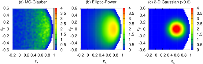
Figure 1: (Color online) (a) Two-dimensional plot of the distribution of $(\varepsilon_{x},\varepsilon_{y})$, with $n=2$, in a Monte Carlo Glauber Alver:2008aq simulation of Pb+Pb collisions at 2.76 TeV per nucleon pair, in the 75-80% centrality range. 40000 events are generated in this centrality. (b) Fit using the Elliptic Power distribution Eq. (3) with $\varepsilon_{0}=0.61$ and $\alpha=3.3$. (c) Fit using an isotropic two-dimensional Gaussian Voloshin:2007pc , corresponding to Eq. (5) with $\varepsilon_{0}=0.61$ and $\sigma_{x}=\sigma_{y}=0.10$. The z-axis of the right panel has been reduced by 0.6 to match the others. All fit parameters are obtained by standard $\chi^{2}$ fits to the distribution of $\varepsilon_{2}$, see Fig. 2 (a).

II.1 Definition and example

The initial anisotropy in harmonic $n$ is defined in every event by Teaney:2010vd

$$\varepsilon_{n}e^{in\psi_{n}}\equiv-\frac{\int r^{n}e^{ni\varphi}\rho(r,\varphi)r{\rm d}r{\rm d}\varphi}{\int r^{n}\rho(r,\varphi)r{\rm d}r{\rm d}\varphi}.$$ (1)

where $\rho(r,\varphi)$ is the energy density near midrapidity shortly after the collision, and $(r,\varphi)$ are polar coordinates in the transverse plane, in a centered coordinate system, where $\varphi=0$ is the orientation of the reaction plane. In most of this paper, we focus on the second harmonic $n=2$. $\varepsilon_{2}$ is often referred to as the “participant eccentricity” and $\psi_{2}$ as the “participant plane”. This terminology refers to Monte Carlo Glauber models Miller:2007ri , in the context of which these concepts were first introduced Alver:2006wh . Note that $0\leq\varepsilon_{n}\leq 1$ by definition.

The initial anisotropy can also be written in cartesian coordinates:

$$\varepsilon_{n}e^{in\psi_{n}}=\varepsilon_{x}+i\varepsilon_{y}.$$ (2)

$\varepsilon_{x}$ is the anisotropy in the reaction plane. For a symmetric density profile satisfying $\rho(r,\varphi)=\rho(r,-\varphi)$, the definition Eq. (1) implies $\varepsilon_{y}=0$, which in turn implies $\psi_{n}=0$: the participant plane coincides with the reaction plane. This is no longer true in the presence of fluctuations.

Figure 1 (a) displays the distribution of $(\varepsilon_{x},\varepsilon_{y})$, for $n=2$, obtained in a Monte Carlo Glauber simulation of Pb+Pb collisions in the 75-80% centrality range. In this simulation, centrality is defined according the to number of participants. The maximum of the distribution is at a positive value of $\varepsilon_{x}$, reflecting the large reaction plane eccentricity. Fluctuations around the most probable value are large. They display characteristic features:

1. The width around the maximum is larger along the $y$ axis than along the $x$ axis.

2. The distribution of $\varepsilon_{x}$ is left skewed with a steeper decrease to the right of the maximum toward a cut-off at $\varepsilon_{2}=1$.

The usual Bessel-Gaussian parametrization Voloshin:2007pc assumes that fluctuations are Gaussian and isotropic and therefore misses both features (see Fig. 1 (c)). These features can be traced back to the constraint that the support of the distribution is the unit disk $\varepsilon_{2}\leq 1$. Our goal in this paper is to derive a generic distribution with these features.

II.2 Two-dimensional distribution

In Ref. Ollitrault:1992bk , an exact expression for the distribution of $(\varepsilon_{x},\varepsilon_{y})$ for $n=2$ was derived under the following assumptions:

• The energy profile is a superposition of $N$ pointlike, identical sources: $\rho({\bf x})\propto\sum_{j=1}^{N}\delta({\bf x}-{\bf x}_{j})$, where ${\bf x}_{j}$ denotes the transverse position of the sources.

• The positions of the sources ${\bf x}_{j}$ are independent.

• The distribution of ${\bf x}_{j}$ is a 2-dimensional Gaussian, where the widths along $x$ and $y$ may differ. Here we denote by $\varepsilon_{0}\equiv\langle y_{j}^{2}-x_{j}^{2}\rangle/\langle y_{j}^{2}+x_{j}^{2}\rangle$ the ellipticity parameter, corresponding to the eccentricity of the distribution of sources in the reaction plane. It satisfies $|\varepsilon_{0}|\leq 1$.

Under these conditions, the distribution of $(\varepsilon_{x},\varepsilon_{y})$ is

$$p(\varepsilon_{x},\varepsilon_{y})=\frac{\alpha}{\pi}(1-\varepsilon_{0}^{2})^{\alpha+\frac{1}{2}}\frac{(1-\varepsilon_{x}^{2}-\varepsilon_{y}^{2})^{\alpha-1}}{(1-\varepsilon_{0}\varepsilon_{x})^{2\alpha+1}},$$ (3)

where $\alpha=(N-1)/2$. This probability distribution is normalized: $\int p(\varepsilon_{x},\varepsilon_{y})d\varepsilon_{x}d\varepsilon_{y}=1$, where integration runs over the unit disk $\varepsilon_{x}^{2}+\varepsilon_{y}^{2}\leq 1$.

In this paper, we argue that Eq. (3), which we name the Elliptic Power distribution, provides a good fit to all models of the initial state. This success can be ascribed to the fact that the natural support of the Elliptic Power distribution is the unit disk: this is a major advantage over previous parametrizations. We treat both the ellipticity $\varepsilon_{0}$ and the power $\alpha$ as fit parameters. In particular, we allow for arbitrary real, positive values of $\alpha$ (as opposed to integer or half-integer).

For $\varepsilon_{0}=0$, the distribution Eq. (3) is azimuthally symmetric:

$$p(\varepsilon_{x},\varepsilon_{y})=\frac{\alpha}{\pi}(1-\varepsilon_{x}^{2}-\varepsilon_{y}^{2})^{\alpha-1}.$$ (4)

This is the one-parameter Power distribution introduced in Ref. Yan:2013laa , which was shown to fit Monte Carlo results when the eccentricity is solely created by fluctuations, as for instance in p-p collisions or p-Pb collisions. The power parameter $\alpha$ quantifies the magnitude of fluctuations: the smaller $\alpha$, the larger the fluctuations.

When the ellipticity $\varepsilon_{0}$ is positive, the denominator of Eq. (3) breaks azimuthal symmetry and favors larger values of $\varepsilon_{x}$. The mean eccentricity in the reaction plane $\varepsilon_{\rm{RP}}\equiv\langle\varepsilon_{x}\rangle$ is derived in Appendix A as a function of $\varepsilon_{0}$ and $\alpha$. Because of fluctuations, it is not strictly equal to the eccentricity of the underlying distribution, $\varepsilon_{0}$ Bhalerao:2006tp . It is in general smaller, and coincides with $\varepsilon_{0}$ only in the limit $\alpha\gg 1$.

A fit to Monte Carlo Glauber results using the Elliptic Power distribution is displayed in Fig. 1 (b). The fit is not perfect. Specifically, the maximum density is slightly overestimated, while the width of the $\varepsilon_{y}$ distribution is slightly underestimated. Note that there are several differences between the ideal case considered in Ollitrault:1992bk and the actual Glauber calculation, specifically: the correlations between the participants, the fact that their distribution in the transverse plane is not a Gaussian, and the recentering correction. We have checked that switching off the recentering correction does not make agreement significantly better. Despite these imperfections, the Elliptic Power distribution captures both features pointed out at the end of Sec. II.1, namely, a larger width along the $y$ axis, and a steeper decrease to the right of the maximum.

The Elliptic Power distribution can be somewhat simplified in the limit $\alpha\gg 1$, corresponding to a large system with small fluctuations. To leading order in $1/\alpha$, Eq. (3) reduces to a two-dimensional elliptic Gaussian distribution:

$$p(\varepsilon_{x},\varepsilon_{y})=\frac{1}{2\pi\sigma_{x}\sigma_{y}}\exp\left(-\frac{(\varepsilon_{x}-\varepsilon_{0})^{2}}{2\sigma_{x}^{2}}-\frac{\varepsilon_{y}^{2}}{2\sigma_{y}^{2}}\right).$$ (5)

The maximum lies on the $x$-axis at $\varepsilon_{x}=\varepsilon_{0}$ and the widths are given by

$$\sigma_{x} = \frac{1-\varepsilon_{0}^{2}}{\sqrt{2\alpha}}$$ (6)

$$\sigma_{y} = \sqrt{\frac{1-\varepsilon_{0}^{2}}{2\alpha}}.$$ (7)

In general, the Gaussian is more elongated along the $y$ axis, that is, $\sigma_{x}<\sigma_{y}$, which corresponds to the first of the two properties listed in Sec. II.1. It is symmetric around its maximum and therefore does not possess the second property, namely, the skewness along the $x$ axis. This property only appears as a next-to-leading correction of order $1/\alpha$, which is derived in Appendix B.

The usual isotropic Gaussian distribution introduced in Ref. Voloshin:2007pc is obtained by setting $\sigma_{x}=\sigma_{y}=\sigma$ in Eq. (5). This parametrization misses both properties and is therefore less accurate than our new Elliptic Power distribution, as can be seen in Fig. 1 (c). In particular, it overestimates the density at the maximum by a factor larger than 2.

II.3 Radial distribution

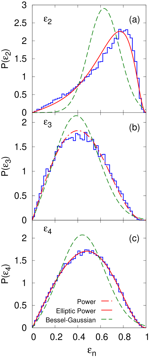
Figure 2: (Color online) Distribution of $\varepsilon_{n}$ in 75–80% central Pb-Pb collisions. (a): $\varepsilon_{2}$, (b): $\varepsilon_{3}$, (c): $\varepsilon_{4}$. Histograms are Monte Carlo Glauber simulations (same as in Fig. 1 (a)). Dashed lines are Bessel-Gaussian fits using Eq.  (14). Full lines are Elliptic Power fits using Eq. (10) for $\varepsilon_{2}$ (parameters as in Fig. 1 (b)) and $\varepsilon_{4}$ ($\alpha=3.2$ and $\varepsilon_{0}=0.22$). The dash-dotted line for $\varepsilon_{3}$ is a Power fit using Eq. (13) ($\alpha=3.6$).

Since the orientation of the reaction plane is not directly accessible experimentally, the magnitude of the eccentricity $\varepsilon_{n}$ matters more than its phase $\varphi\equiv n\psi_{n}$. Monte Carlo simulations of the initial state typically return a probability distribution $P(\varepsilon_{n})$ for each centrality Aad:2013xma ; Schenke:2013aza ; Yan:2013laa . It is obtained by transforming $p(\varepsilon_{x},\varepsilon_{y})$ to polar coordinates and integrating over the azimuthal angle:

$$P(\varepsilon_{n})\equiv\varepsilon_{n}\int_{0}^{2\pi}p(\varepsilon_{n}\cos\varphi,\varepsilon_{n}\sin\varphi)d\varphi.$$ (8)

It is normalized by construction: $\int_{0}^{1}P(\varepsilon_{n})d\varepsilon_{n}=1$. Inserting Eq. (3) into Eq. (8) and using the symmetry of the integrand under $\varphi\to-\varphi$, one obtains

$$P(\varepsilon_{n}) = 2\alpha\varepsilon_{n}(1-\varepsilon_{n}^{2})^{\alpha-1}(1-\varepsilon_{0}^{2})^{\alpha+\frac{1}{2}}$$ (10)

$$\times\frac{1}{\pi}\int_{0}^{\pi}(1-\varepsilon_{0}\varepsilon_{n}\cos\varphi)^{-2\alpha-1}d\varphi.$$

The integral can be carried out analytically to give

$$P(\varepsilon_{n}) = 2\varepsilon_{n}\alpha(1-\varepsilon_{n}^{2})^{\alpha-1}(1-\varepsilon_{n}\varepsilon_{0})^{-1-2\alpha}(1-\varepsilon_{0}^{2})^{\alpha+\frac{1}{2}}\times$$ (12)

$${{}_{2}}F_{1}\left(\frac{1}{2},1+2\alpha;1;\frac{2\varepsilon_{n}\varepsilon_{0}}{\varepsilon_{n}\varepsilon_{0}-1}\right).$$

However, if the hypergeometric function is not available, or not defined everywhere needed, the integral over angles in Eq. (10) may be carried out numerically.

For $\varepsilon_{0}=0$, Eq. (10) reduces to

$$P(\varepsilon_{n})=2\alpha\varepsilon_{n}(1-\varepsilon_{n}^{2})^{\alpha-1},$$ (13)

which is the “Power” distribution Yan:2013laa . In the limit $\alpha\gg 1$ this becomes a Gaussian. In the limit $\alpha\gg 1$ and $\varepsilon_{0}\ll 1$, Eqs. (5) and (8) give

$$P(\varepsilon_{n})=\frac{\varepsilon_{n}}{\sigma^{2}}\exp\left(-\frac{\varepsilon_{n}^{2}+\varepsilon_{0}^{2}}{2\sigma^{2}}\right)I_{0}\left(\frac{\varepsilon_{0}\varepsilon_{n}}{\sigma^{2}}\right),$$ (14)

which is the usual Bessel-Gaussian distribution Voloshin:2007pc , where we have defined $\sigma\equiv 1/\sqrt{2\alpha}$. Note that if $\sigma_{x}\not=\sigma_{y}$, the two-dimensional elliptic Gaussian distribution Eq. (5) does not give the Bessel-Gaussian distribution upon integration over $\varphi$ Ollitrault:1992bk .

Figure 2 (a) presents the histogram of $\varepsilon_{2}$ obtained by integrating the results of Fig. 1 (a) over azimuthal angle. The fit using the Elliptic Power distribution is clearly much better than the fit using the Bessel-Gaussian.

For sake of completeness, Fig. 2 (b) and (c) also display the distributions of higher order Fourier harmonics $\varepsilon_{3}$ and $\varepsilon_{4}$. The initial triangularity $\varepsilon_{3}$ acts as a seed for triangular anisotropy Alver:2010gr , in the same way as the initial eccentricity is the origin of elliptic anisotropy. Since triangularity is solely created by fluctuations, the distribution of $\varepsilon_{3}$ is well reproduced by the single-parameter Power distribution, Eq. (13) Yan:2013laa . If the two-parameter Elliptic Power distribution is used for $\varepsilon_{3}$, the $\varepsilon_{0}$ parameter comes out to be essentially zero. The one-parameter fit is significantly better than the two-parameter Bessel-Gaussian fit, Eq. (14). Note that the values of $\alpha$ are not necessarily the same for ellipticity and triangularity. The distribution of the fourth harmonic $\varepsilon_{4}$ is well fitted by the Elliptic Power distribution. The resulting value of $\varepsilon_{0}$ is significantly smaller than for the distribution of $\varepsilon_{2}$. Note, however, that the $\varepsilon_{0}$ for $\varepsilon_{4}$ is not the only origin of anisotropy in the corresponding harmonic, due to large nonlinear terms in the hydrodynamic response Teaney:2010vd ; Gardim:2011xv ; Teaney:2012ke .

Figure 3: (Color online) Histograms of the distribution of $\varepsilon_{2}$ in Pb+Pb collisions at 2.76 TeV using the PHOBOS Monte Carlo Glauber Alver:2008aq (panels (a) to (d)) and the IP-Glasma Schenke:2013aza ; Schenke:2014tga (panels (e) to (h)) for four centrality bins (with decreasing centrality or increasing centrality percentile from left to right). Solid curves are fits using the Elliptic Power distribution, Eq. (10), dashed curves are fits using the Bessel-Gaussian distribution, Eq. (14). Each bin contains $\sim$40000 events for the Glauber simulation, and $\sim$2000 events for the IP-Glasma, which explains the larger statistical fluctuations for the bottom row even though the bins are twice as wide. The area under the curves is $0.5$ for the 5-10% centrality bin and $1$ for the other bins.

III Analyzing Monte Carlo models of Pb+Pb collisions

Figure 4: (Color online) (a): Power parameter $\alpha$ from Elliptic Power fits to the eccentricity distribution and Power fits to the triangularity distribution [cf. Fig. 2 (b)], as a function of centrality for the Monte Carlo Glauber model Alver:2008aq and the IP-Glasma model Schenke:2013aza . (b): Symbols correspond to the value of the ellipticity parameter $\varepsilon_{0}$. Lines correspond to the mean eccentricity in the reaction plane $\varepsilon_{\rm{RP}}$ for the Glauber model, either calculated directly (full line), or estimated using the Elliptic Power distribution Eq. (23) (dotted line).

III.1 Histograms

We now argue that the Elliptic Power distribution always gives good fits to distributions of $\varepsilon_{2}$ in nucleus-nucleus collisions. Figure 3 presents the histogram of $\varepsilon_{2}$ in Pb+Pb at 2.76 TeV in several centrality bins, obtained using the Monte Carlo Glauber (panels (a) to (d)) Alver:2008aq and the IP-Glasma (panels (e) to (h)) Schenke:2012hg models, together with fits using the Elliptic Power and the Bessel-Gaussian distributions. Both distributions are able to fit both models in the 5-10% centrality bin. Bessel-Gaussian fits become worse as the centrality percentile is increased, while Elliptic Power fits are excellent for both models and for all centralities. Only four centrality bins are shown in Fig. 3 for sake of illustration, but we have checked that the fits are as good for the other centralities. For the most central bin (0-5%), however, the fit parameters are strongly correlated and cannot be determined independently. This can be understood as follows: for central collisions, the Elliptic Power distribution is very close to a Bessel-Gaussian distribution, Eq. (14). Now, to order $\varepsilon_{0}^{2}$, this distribution is invariant under the transformation $(\sigma^{2},\varepsilon_{0})\to(\sigma^{2}+\varepsilon_{0}^{2}/2,0)$, i.e, the dependence on $\varepsilon_{0}$ can be absorbed into a redefinition of the width $\sigma$. Therefore one cannot fit $\varepsilon_{0}$ and $\sigma$ independently when $\varepsilon_{0}$ is too small and one can actually use the one-parameter Power distribution.

The two models plotted in Fig. 3 represent two extremes in the landscape of initial-state models. The PHOBOS Monte Carlo model is the simplest model including fluctuations: all participant nucleons are treated as identical, pointlike sources of energy. By contrast, in the IP-Glasma model, the energy density is treated as a continuous field and contains nontrivial fluctuations at the subnucleonic level. The Elliptic Power distribution is able to fit both extremes. We have explicitly checked that it works well also for the MC-KLN model Drescher:2007ax . We therefore conjecture that it provides a good fit to all Monte Carlo models of initial conditions.

III.2 Power parameter and Ellipticity

The Elliptic Power distribution, Eq. (3), encodes the information about the eccentricity distribution into two parameters which are plotted in Fig. 4 as a function of centrality for the IP Glasma and Monte Carlo Glauber models. As explained above, the two parameters cannot be disentangled for very central collisions — in practice, the fitting procedure returns a very large error on each parameter: therefore we exclude the most central ($0-5\%$) bin. Panel (a) also displays the values of $\alpha$ obtained by fitting the distribution of the triangularity $\varepsilon_{3}$ with the Power distribution Eq. (13). The power parameter $\alpha$ increases towards central collisions. This is expected, since $\alpha$ is typically proportional to the system size. In the Monte Carlo Glauber model, $\alpha$ is approximately proportional to the number of participant nucleons $N_{\rm part}$.

The ellipticity $\varepsilon_{0}$, on the other hand, smoothly increases with centrality percentile, and is somewhat larger for the IP-Glasma than for the Glauber model, in line with the expectations that saturation-inspired models predict a larger eccentricity than Glauber models Lappi:2006xc . For the Monte Carlo Glauber model, we also show on the same plot the reaction plane eccentricity $\varepsilon_{\rm{RP}}$: we can either calculate it directly in the Monte Carlo Glauber model (full line) or estimate it using Eq. (23) below derived from the Elliptic Power distribution (dotted line). It is close to the Glauber $\varepsilon_{0}$ up to mid-centrality. The difference between $\varepsilon_{0}$ and $\varepsilon_{\rm{RP}}$ is nevertheless much larger than predicted by the Elliptic Power distribution. This can be attributed to the fact that the Elliptic Power distribution does not reproduce all the fine structure of the two-dimensional distribution (Fig. 1 (a)), even though it provides a very good fit to the distribution of $\varepsilon_{2}$ (Figs. 2 (a) and 3).

III.3 Fluctuations

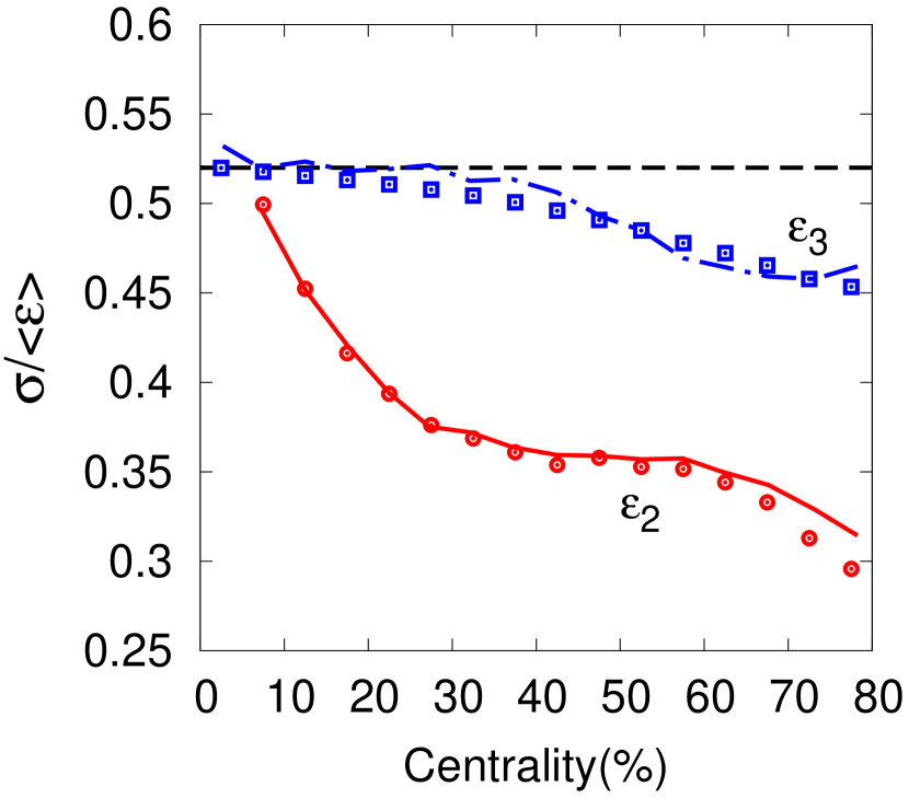
Figure 5: (Color online) Relative fluctuations, as defined by Eq. (15), as a function of collision centrality. Lines: Monte Carlo Glauber results for $\varepsilon_{2}$ (full) and $\varepsilon_{3}$ (dash-dotted). Symbols are results using the Elliptic Power distribution Eq. (10) for $\varepsilon_{2}$ (circles), and the Power distribution Eq. (13) for $\varepsilon_{3}$ (squares), with parameters fitted to the histograms. The horizontal dashed line indicates the value $\sqrt{4/\pi-1}$ corresponding to pure Gaussian fluctuations (Eq. (14) with $\varepsilon_{0}$).

A standard measure of eccentricity fluctuations is the ratio of the standard deviation to the mean Miller:2007ri ; Sorensen:2006nw :

$$\frac{\sigma_{\varepsilon_{n}}}{\langle\varepsilon_{n}\rangle}=\frac{\sqrt{\langle\varepsilon_{n}^{2}\rangle-\langle\varepsilon_{n}\rangle^{2}}}{\langle\varepsilon_{n}\rangle},$$ (15)

where angular brackets denote an average over events in a centrality class. We now check that the Elliptic Power distribution, fitted to the histogram of $\varepsilon_{2}$, correctly reproduces the magnitude of eccentricity fluctuations.

The ratio Eq. (15) is presented in Fig. 5 for $\varepsilon_{2}$ and $\varepsilon_{3}$. For central collisions, it approaches $\sqrt{4/\pi-1}\simeq 0.52$ Broniowski:2007ft for both $\varepsilon_{2}$ and $\varepsilon_{3}$, which is the value given by Eq. (14) for $\varepsilon_{0}=0$. For more peripheral collisions, relative eccentricity fluctuations decrease very mildly for $\varepsilon_{3}$, and more strongly for $\varepsilon_{2}$. For $\varepsilon_{3}$, this mild decrease is captured by fitting with the Power distribution, Eq. (13). The mean of the Power distribution is given by

$$\langle\varepsilon_{3}\rangle=\frac{\sqrt{\pi}\,\Gamma(\alpha+1)}{2\,\Gamma(\alpha+\frac{3}{2})},$$ (16)

while the mean square is Yan:2013laa $\langle\varepsilon_{3}^{2}\rangle=1/(\alpha+1)$.

The mean of the Elliptic Power distribution, Eq. (10), must be calculated numerically as a function of $\varepsilon_{0}$ and $\alpha$. The eccentricity fluctuations from the Elliptic Power distribution closely match the Monte Carlo Glauber result in Fig. 5.

III.4 Cumulants

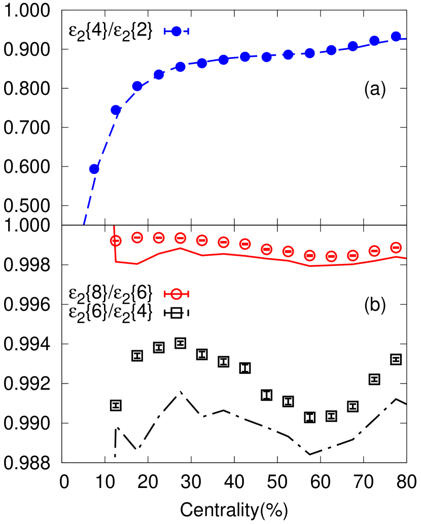
Figure 6: (Color online) (a): Cumulant ratio $\varepsilon_{2}\{4\}/\varepsilon_{2}\{2\}$. (b): Cumulant ratios $\varepsilon_{2}\{6\}/\varepsilon_{2}\{4\}$ and $\varepsilon_{2}\{8\}/\varepsilon_{2}\{6\}$. Lines are Monte Carlo Glauber results. Symbols are results using the Elliptic Power distribution Eq. (27) with parameters fitted to the distribution of $\varepsilon_{2}$.

More detailed information about eccentricity fluctuations is contained in moments or cumulants of the distribution. The moment of order $k$ is defined as $\langle(\varepsilon_{n})^{k}\rangle$. Often, one solely uses even moments of the distribution $\langle(\varepsilon_{n})^{2k}\rangle$, because the corresponding moments of the distribution of anisotropic flow are directly accessible through cumulant analyses Borghini:2001vi ; Bilandzic:2010jr . The first eccentricity cumulants Miller:2003kd ; Bzdak:2013rya are defined by:

$$\varepsilon_{n}\{2\} \equiv \langle\varepsilon_{n}^{2}\rangle^{1/2}$$ (17)

$$\varepsilon_{n}\{4\} \equiv \left(2\langle\varepsilon_{n}^{2}\rangle^{2}-\langle\varepsilon_{n}^{4}\rangle\right)^{1/4}$$ (18)

$$\varepsilon_{n}\{6\} \equiv \left(\frac{\langle\varepsilon_{n}^{6}\rangle-9\langle\varepsilon_{n}^{2}\rangle\langle\varepsilon_{n}^{4}\rangle+12\langle\varepsilon_{n}^{2}\rangle^{3}}{4}\right)^{1/6}.$$ (19)

Figure 6 displays ratios of successive cumulants obtained in the Monte Carlo Glauber calculation and using the Elliptic Power distribution, Eq. (27). $\varepsilon_{2}\{4\}/\varepsilon_{2}\{2\}$ increases from central to peripheral collisions. It is smaller than unity by definition. Higher order ratios $\varepsilon_{2}\{6\}/\varepsilon_{2}\{4\}$ and $\varepsilon_{2}\{8\}/\varepsilon_{2}\{6\}$ are exactly equal to 1 for the Bessel-Gaussian distribution. The Monte Carlo Glauber calculation gives ratios slightly smaller than unity, with a nontrivial centrality dependence. These nontrivial features are reproduced by the Elliptic Power distribution.

IV Conclusions

We have introduced a new parametrization of the eccentricity distribution in nucleus-nucleus collisions. Like the previously used Bessel-Gaussian parametrization, it is a two-parameter distribution, but it describes peripheral collisions much better. This is due to the correct implementation of the constraint that the eccentricity must be smaller than unity in all events. The consequence of our result is that any model of initial-state eccentricities can be characterized by two numbers for each centrality: the ellipticity $\varepsilon_{0}$, which corresponds closely to the reaction-plane eccentricity; the power parameter $\alpha$, which governs the magnitude of fluctuations and scales like the number of participants in the Glauber model.

Since elliptic flow is essentially proportional to the initial eccentricity Niemi:2012aj , our result can be applied Yan2014 to the distribution of elliptic flow values, which has been measured recently at the LHC Aad:2013xma ; Jia:2013tja . The Elliptic Power distribution could also be used as a kernel in the unfolding procedure which is used to eliminate finite multiplicity fluctuations Alver:2007qw . It could also be used in fitting the distribution of the flow vector Barrette:1994xr ; Voloshin:1994mz ; Adler:2002pu . We expect it to give a better result than the Bessel-Gaussian distribution, which has been found to be not precise for peripheral collisions Aad:2013xma .

Appendix A Mathematical properties of the Elliptic Power distribution

The two-dimensional Elliptic Power distribution Eq. (3) is normalized to unity on the unit disk if $\alpha>0$ and $-1<\varepsilon_{0}<1$. We choose the convention $\varepsilon_{0}\geq 0$ throughout this paper.

For $\alpha\geq 1$, Eq. (3) has a maximum on the $x$-axis for $\varepsilon_{x}=\varepsilon_{\rm max}$, where

$$\varepsilon_{\rm max}\equiv\frac{\varepsilon_{0}(1+2\alpha)}{\alpha-1+\sqrt{(\alpha-1)^{2}+3\varepsilon_{0}^{2}(1+2\alpha)}}.$$ (20)

But for $0<\alpha<1$, the distribution diverges on the unit circle $\varepsilon_{x}^{2}+\varepsilon_{y}^{2}=1$.

The mean eccentricity in the reaction plane is obtained by integrating Eq. (3):

$$\varepsilon_{\rm{RP}} = \int_{-1}^{+1}\varepsilon_{x}d\varepsilon_{x}\int_{-\sqrt{1-\varepsilon_{x}^{2}}}^{\sqrt{1-\varepsilon_{x}^{2}}}d\varepsilon_{y}p(\varepsilon_{x},\varepsilon_{y})$$ (21)

$$= \frac{\alpha+\frac{1}{2}}{\alpha+1}\varepsilon_{0}(1-\varepsilon_{0}^{2})^{\alpha+\frac{1}{2}}\times$$ (23)

$${{}_{2}}F_{1}\left(\alpha+1,\alpha+\frac{3}{2};\alpha+2;\varepsilon_{0}^{2}\right),$$

where ${}_{2}F_{1}$ denotes the hypergeometric function. In the limit $\varepsilon_{0}\ll 1$, it simplifies to

$$\varepsilon_{\rm{RP}}=\frac{\alpha+\frac{1}{2}}{\alpha+1}\varepsilon_{0}+{\cal O}(\varepsilon_{0}^{3}).$$ (24)

Thus $\varepsilon_{0}$ is slightly bigger than $\varepsilon_{\rm{RP}}$ due to fluctuations.

We now explain how to evaluate the moments of the Elliptic Power distribution. Multiplying Eq. (3) by $(1-\varepsilon_{x}^{2}+\varepsilon_{y}^{2})^{k}$ and integrating successively over $\varepsilon_{y}$ and $\varepsilon_{x}$, one obtains

$$\langle(1-\varepsilon_{n}^{2})^{k}\rangle = \frac{\alpha}{\alpha+k}\left(1-\varepsilon_{0}^{2}\right)^{k}\times$$ (26)

$${{}_{2}}F_{1}\left(k+\frac{1}{2},k;\alpha+k+1;\varepsilon_{0}^{2}\right).$$

Using this equation, one can express analytically the even moments $\langle\varepsilon_{n}^{2k}\rangle$ and the cumulants Bzdak:2013rya $\varepsilon_{n}\{2k\}$ as a function of $\alpha$ and $\varepsilon_{0}$. Using the shorthand notation $f_{k}\equiv\langle(1-\varepsilon_{n}^{2})^{k}\rangle$ and inserting into Eq. (17), one obtains

$$\varepsilon_{n}\{2\} = (1-f_{1})^{1/2}$$ (27)

$$\varepsilon_{n}\{4\} = (1-2f_{1}+2f_{1}^{2}-f_{2})^{1/4}$$ (28)

$$\varepsilon_{n}\{6\} = \left(1+\frac{9}{2}f_{1}^{2}-3f_{1}^{3}+3f_{1}(\frac{3}{4}f_{2}-1)-\frac{3}{2}f_{2}\right.$$ (30)

$$\left.-\frac{1}{4}f_{3}\right)^{1/6}.$$

Appendix B Limiting distribution for fixed $\varepsilon_{0}>0$ and $\alpha\gg 1$

We now study the Elliptic Power distribution Eq. (3) in the limit $\alpha\gg 1$, corresponding to a large system. To leading order, the distribution is a Gaussian centered around the intrinsic ellipticity $\varepsilon_{0}$, see Eq. (5). We therefore write $\varepsilon_{x}=\varepsilon_{0}+\delta_{x}$ and treat $\delta_{x}$ and $\varepsilon_{y}$ as small parameters of order $\sigma_{x}\sim\sigma_{y}\sim\alpha^{-1/2}$. Expanding the logarithm of Eq. (3) in powers of $\alpha^{-1/2}$ and exponentiating, one obtains

$$p(\varepsilon_{0}+\delta_{x},\varepsilon_{y})=p_{0}(\varepsilon_{0}+\delta_{x},\varepsilon_{y})\left(1+W_{1}+W_{3}\right),$$ (31)

where $p_{0}$ is the Gaussian distribution in Eq. (5), and $W_{1}$ and $W_{3}$ are perturbations of order $\alpha^{-1/2}$:

$$W_{1} \equiv \frac{3\varepsilon_{0}\delta_{x}}{1-\varepsilon_{0}^{2}}$$ (32)

$$W_{3} \equiv -\left(\frac{\delta_{x}^{2}}{\sigma_{x}^{2}}+\frac{\varepsilon_{y}^{2}}{\sigma_{y}^{2}}\right)\frac{\varepsilon_{0}\delta_{x}}{1-\varepsilon_{0}^{2}}.$$ (33)

$W_{1}$ is linear, while $W_{3}$ is cubic in $\delta_{x}$ and $\varepsilon_{y}$. The linear term $W_{1}$ shifts the maximum of the distribution, which is found by setting $\varepsilon_{y}\equiv 0$ in Eq. (31) and differentiating with respect to $\delta_{x}$:

$$\varepsilon_{\rm max}=\varepsilon_{0}+\frac{3\varepsilon_{0}(1-\varepsilon_{0}^{2})}{2\alpha}+{\cal O}\left(\frac{1}{\alpha^{2}}\right).$$ (34)

Alternatively, this result can be recovered by expanding Eq. (20).

The cubic term $W_{3}$ skews the Gaussian and is responsible for the skewness seen in Fig. 1 (b) and Fig. 2 (a). The linear term $W_{1}$ can be absorbed by shifting the maximum of the Gaussian according to Eq. (34), therefore the difference between $\varepsilon_{\rm{RP}}$ and $\varepsilon_{\rm max}$ is solely due to $W_{3}$:

$$\varepsilon_{\rm{RP}} = \varepsilon_{\rm max}+\int p_{0}(\varepsilon_{0}+\delta_{x},\varepsilon_{y})W_{3}\delta_{x}d\delta_{x}d\varepsilon_{y}$$ (35)

$$= \varepsilon_{0}-\frac{\varepsilon_{0}(1-\varepsilon_{0}^{2})}{2\alpha}+{\cal O}\left(\frac{1}{\alpha^{2}}\right).$$ (36)

Comparing with Eq. (34), one sees that $\varepsilon_{\rm{RP}}<\varepsilon_{\rm max}$, which is a consequence of the skewness. Alternatively, Eq. (35) can be obtained by expanding Eq. (23).

The first moments can also be evaluated to first order in $1/\alpha$. The mean square eccentricity is

$$\varepsilon_{n}\{2\}^{2}=\langle\varepsilon_{n}^{2}\rangle=\varepsilon_{0}^{2}+\frac{(1-\varepsilon_{0}^{2})\left(1-\frac{3}{2}\varepsilon_{0}^{2}\right)}{\alpha}+{\cal O}\left(\frac{1}{\alpha^{2}}\right).$$ (37)

When $\varepsilon_{0}\to 0$, one recovers the result obtained with the Power distribution Yan:2013laa in the limit $\alpha\gg 1$. When $\varepsilon_{0}>\sqrt{\frac{2}{3}}\simeq 0.816$, the correction is negative, so that rms anisotropy is smaller than $\varepsilon_{0}$. The fourth moment is given by

$$\langle\varepsilon_{n}^{4}\rangle=\varepsilon_{0}^{4}+\frac{\varepsilon_{0}^{2}(1-\varepsilon_{0}^{2})(4-5\varepsilon_{0}^{2})}{\alpha}+{\cal O}\left(\frac{1}{\alpha^{2}}\right).$$ (38)

From Eqs. (37) and (38), one obtains the cumulant $\varepsilon_{n}\{4\}$ (see Eq. (17)):

$$\varepsilon_{n}\{4\}=\varepsilon_{0}-\frac{\varepsilon_{0}(1-\varepsilon_{0}^{2})}{4\alpha}+{\cal O}\left(\frac{1}{\alpha^{2}}\right).$$ (39)

Note that $\varepsilon_{n}\{4\}<\varepsilon_{0}$ for all positive $\varepsilon_{0}$ in the limit $\alpha\gg 1$. In the limiting case $\varepsilon_{0}=0$, $\varepsilon_{n}\{4\}^{4}$ is positive and of order $\alpha^{-3}$ Yan:2013laa . Higher order cumulants are all equal to $\varepsilon_{n}\{4\}$ to order $1/\alpha$.

Appendix C Limiting distribution for fixed $\alpha\varepsilon_{0}^{2}$ and $\alpha\gg 1$

We now consider a different asymptotic expansion introduced in Alver:2008zza , where one treats $\alpha$ as a large parameter and $\varepsilon_{0}$ as a small parameter, keeping the product $\alpha\varepsilon_{0}^{2}$ fixed. The only difference with the asymptotic expansion carried out in Appendix B is that we also treat $\varepsilon_{0}$ as a small parameter of order $\alpha^{-1/2}$. Therefore the perturbations $W_{1}$ and $W_{3}$ in Eq. (32) are of order $\alpha^{-1}$. For sake of consistency, one must carry out the whole expansion to that order. One obtains

$$p(\varepsilon_{0}+\delta_{x},\varepsilon_{y})=p_{0}(\varepsilon_{0}+\delta_{x},\varepsilon_{y})\left(1+W_{1}+W_{3}+W_{4}\right),$$ (40)

where $W_{1}$ and $W_{3}$ are defined in Eq. (32) and $W_{4}$ is a new quartic term:

$$W_{1} \equiv 3\varepsilon_{0}\delta_{x}$$ (41)

$$W_{3} \equiv -2\alpha\varepsilon_{0}\delta_{x}\vec{\delta}^{2}$$ (42)

$$W_{4} \equiv -\frac{\alpha}{2}(\vec{\delta}^{2})^{2}+\vec{\delta}^{2},$$ (43)

where we have introduced the shorthand notation $\vec{\delta}^{2}\equiv\delta_{x}^{2}+\varepsilon_{y}^{2}$ and simplified the expressions of $W_{1}$ and $W_{3}$ using Eq. (6) and $\varepsilon_{0}\ll 1$. In the isotropic case $\varepsilon_{0}=0$, both $W_{1}$ and $W_{3}$ vanish and only $W_{4}$ contributes.

The mean square eccentricity is given by

$$\varepsilon_{n}\{2\}^{2}=\varepsilon_{0}^{2}+\frac{1}{\alpha}-\frac{5\varepsilon_{0}^{2}}{2\alpha}-\frac{1}{\alpha^{2}}+{\cal O}\left(\frac{1}{\alpha^{3}}\right),$$ (44)

where the first two terms are the leading order terms, of order $1/\alpha$, and the two next terms are corrections of order $1/\alpha^{2}$. The first three terms are present in Eq. (37), while the last term is the contribution of the quartic perturbation $W_{4}$ in Eq. (41). Similarly, one can expand the cumulant $\varepsilon_{n}\{4\}$, to give for the fourth power:

$$\varepsilon_{n}\{4\}^{4}=\varepsilon_{0}^{4}-\frac{\varepsilon_{0}^{4}}{\alpha}+\frac{8\varepsilon_{0}^{2}}{\alpha^{2}}+\frac{2}{\alpha^{3}}+{\cal O}\left(\frac{1}{\alpha^{4}}\right),$$ (45)

where the first term is the leading term, of order $1/\alpha^{2}$, and the next three terms are corrections of order $1/\alpha^{3}$. In the isotropic case $\varepsilon_{0}=0$, the exact result is $\varepsilon_{n}\{4\}^{4}=2/[(\alpha+1)^{2}(\alpha+2)]$ Yan:2013laa , which reduces to $\varepsilon_{n}\{4\}^{4}\simeq 2/\alpha^{3}$ for $\alpha\gg 1$, in agreement with the above result.

Ratios of cumulants are given to leading order by:

$$\frac{\varepsilon\{4\}}{\varepsilon\{2\}} = \sqrt{\frac{\alpha\varepsilon_{0}^{2}}{1+\alpha\varepsilon_{0}^{2}}}+{\cal O}\left(\frac{1}{\alpha}\right)$$ (46)

$$\frac{\varepsilon\{6\}}{\varepsilon\{4\}} = 1-\frac{1+\alpha\varepsilon_{0}^{2}}{2(\alpha\varepsilon_{0}^{2})^{2}\alpha}+{\cal O}\left(\frac{1}{\alpha^{2}}\right)$$ (47)

$$\frac{\varepsilon\{8\}}{\varepsilon\{6\}} = 1-\frac{1}{22(\alpha\varepsilon_{0}^{2})\alpha}+{\cal O}\left(\frac{1}{\alpha^{2}}\right).$$ (48)

References

- (1) K. H. Ackermann et al. [STAR Collaboration], Phys. Rev. Lett. 86, 402 (2001)
- (2) S. S. Adler et al. [PHENIX Collaboration], Phys. Rev. Lett. 91, 182301 (2003)
- (3) KAamodt et al. [ALICE Collaboration], Phys. Rev. Lett. 105, 252302 (2010)
- (4) G. Aad et al. [ATLAS Collaboration], Phys. Lett. B 707, 330 (2012)
- (5) S. Chatrchyan et al. [CMS Collaboration], Phys. Rev. C 87, 014902 (2013)
- (6) P. Romatschke and U. Romatschke, Phys. Rev. Lett. 99, 172301 (2007)
- (7) M. Luzum and P. Romatschke, Phys. Rev. C 78, 034915 (2008) [Erratum-ibid. C 79, 039903 (2009)]
- (8) B. Alver et al. [PHOBOS Collaboration], Phys. Rev. Lett. 98, 242302 (2007)
- (9) T. Hirano, U. W. Heinz, D. Kharzeev, R. Lacey and Y. Nara, Phys. Lett. B 636, 299 (2006)
- (10) T. Lappi and R. Venugopalan, Phys. Rev. C 74, 054905 (2006)
- (11) M. Miller and R. Snellings, [nucl-ex/0312008.]
- (12) M. L. Miller, K. Reygers, S. J. Sanders and P. Steinberg, Ann. Rev. Nucl. Part. Sci. 57, 205 (2007)
- (13) C. Flensburg, arXiv:1108.4862 [nucl-th].
- (14) A. Dumitru and Y. Nara, Phys. Rev. C 85, 034907 (2012)
- (15) B. Schenke, P. Tribedy and R. Venugopalan, Phys. Rev. C 86, 034908 (2012)
- (16) H. Holopainen, H. Niemi and K. J. Eskola, Phys. Rev. C 83, 034901 (2011)
- (17) B. Schenke, S. Jeon and C. Gale, Phys. Rev. Lett. 106, 042301 (2011)
- (18) Z. Qiu and U. W. Heinz, Phys. Rev. C 84, 024911 (2011)
- (19) P. Bozek, Phys. Rev. C 85, 014911 (2012)
- (20) H.-J. Drescher and Y. Nara, Phys. Rev. C 76, 041903 (2007)
- (21) B. Schenke, P. Tribedy and R. Venugopalan, Phys. Rev. Lett. 108, 252301 (2012)
- (22) R. Andrade, F. Grassi, Y. Hama, T. Kodama and O. Socolowski, Jr., Phys. Rev. Lett. 97, 202302 (2006)
- (23) Z. -W. Lin, C. M. Ko, B. -A. Li, B. Zhang and S. Pal, Phys. Rev. C 72, 064901 (2005)
- (24) H. Petersen, J. Steinheimer, G. Burau, M. Bleicher and H. Stocker, Phys. Rev. C 78, 044901 (2008)
- (25) S. A. Voloshin, A. M. Poskanzer and R. Snellings, arXiv:0809.2949 [nucl-ex].
- (26) S. A. Voloshin, A. M. Poskanzer, A. Tang and G. Wang, Phys. Lett. B 659, 537 (2008)
- (27) L. Yan and J. -Y. Ollitrault, Phys. Rev. Lett. 112, 082301 (2014)
- (28) A. Bzdak, P. Bozek and L. McLerran, Nucl. Phys. A927, 15 (2014)
- (29) A. Bzdak and V. Skokov, arXiv:1312.7349 [hep-ph].
- (30) D. Teaney and L. Yan, Phys. Rev. C 83, 064904 (2011)
- (31) B. Alver, M. Baker, C. Loizides and P. Steinberg, arXiv:0805.4411 [nucl-ex].
- (32) J.-Y. Ollitrault, Phys. Rev. D 46, 229 (1992).
- (33) J. Casalderrey-Solana and U. A. Wiedemann, Phys. Rev. Lett. 104, 102301 (2010)
- (34) S. K. Prasad, V. Roy, S. Chattopadhyay and A. K. Chaudhuri, Phys. Rev. C 82, 024909 (2010)
- (35) R. S. Bhalerao and J. -Y. Ollitrault, Phys. Lett. B 641, 260 (2006)
- (36) G. Aad et al. [ATLAS Collaboration], JHEP 11, 183 (2013)
- (37) B. Schenke, P. Tribedy and R. Venugopalan, Nucl. Phys. A926, 102 (2014)
- (38) B. Alver and G. Roland, Phys. Rev. C 81, 054905 (2010) [Erratum-ibid. C 82, 039903 (2010)]
- (39) F. G. Gardim, F. Grassi, M. Luzum and J. -Y. Ollitrault, Phys. Rev. C 85, 024908 (2012)
- (40) D. Teaney and L. Yan, Phys. Rev. C 86, 044908 (2012)
- (41) B. Schenke, P. Tribedy and R. Venugopalan, arXiv:1403.2232 [nucl-th].
- (42) C. Gale, S. Jeon, B. Schenke, P. Tribedy and R. Venugopalan, Phys. Rev. Lett. 110, 012302 (2013)
- (43) P. Sorensen [STAR Collaboration], J. Phys. G 34, S897 (2007)
- (44) W. Broniowski, P. Bozek and M. Rybczynski, Phys. Rev. C 76, 054905 (2007)
- (45) N. Borghini, P. M. Dinh and J. -Y. Ollitrault, Phys. Rev. C 64, 054901 (2001)
- (46) A. Bilandzic, R. Snellings and S. Voloshin, Phys. Rev. C 83, 044913 (2011)
- (47) H. Niemi, G. S. Denicol, H. Holopainen and P. Huovinen, Phys. Rev. C 87, 054901 (2013)
- (48) L. Yan, J.-Y. Ollitrault, and A. M. Poskanzer, Quark Matter presentation, Darmstadt (2014).
- (49) J. Jia and S. Mohapatra, Phys. Rev. C 88, no. 1, 014907 (2013)
- (50) B. Alver et al. [PHOBOS Collaboration], Phys. Rev. Lett. 104, 142301 (2010)
- (51) J. Barrette et al. [E877 Collaboration], Phys. Rev. Lett. 73, 2532 (1994)
- (52) S. Voloshin and Y. Zhang, Z. Phys. C 70, 665 (1996)
- (53) C. Adler et al. [STAR Collaboration], Phys. Rev. C 66, 034904 (2002)
- (54) B. Alver, B. B. Back, M. D. Baker, M. Ballintijn, D. S. Barton, R. R. Betts, R. Bindel and W. Busza et al., Phys. Rev. C 77, 014906 (2008)