Lensing reconstruction from a patchwork of polarization maps

Abstract

The lensing signals involved in CMB polarization maps have already been measured with ground-based experiments such as SPTpol and POLARBEAR, and would become important as a probe of cosmological and astrophysical issues in the near future. Sizes of polarization maps from ground-based experiments are, however, limited by contamination of long wavelength modes of observational noise. To further extract the lensing signals, we explore feasibility of measuring lensing signals from a collection of small sky maps each of which is observed separately by a ground-based large telescope, i.e., lensing reconstruction from a patchwork map of large sky coverage organized from small sky patches. We show that, although the B-mode power spectrum obtained from the patchwork map is biased due to baseline uncertainty, bias on the lensing potential would be negligible if the B-mode on scales larger than the blowup scale of $1/f$ noise is removed in the lensing reconstruction. As examples of cosmological applications, we also show 1) the cross-correlations between the reconstructed lensing potential and full-sky temperature/polarization maps from satellite missions such as PLANCK and LiteBIRD, and 2) the use of the reconstructed potential for delensing B-mode polarization of LiteBIRD observation.

1 Introduction

The map of cosmic microwave background (CMB) polarization produced from primordial density fluctuations at the cosmic recombination epoch has specific spatial pattern of even parity which is called as E-mode. Mass distribution between the last scattering surface and the Earth bends the path of CMB photons and disturbs the spatial pattern of the polarization map, which violates parity symmetry and induces odd parity pattern (so-called B-mode) (e.g., [1]). Since the gravitational lensing distortion is non-linear effect in terms of perturbation, the lensed polarization map has off-diagonal correlations in angular multipole space which can be utilized for reconstruction of the gravitational lensing potential. The CMB polarization provides a powerful probe of the lensing mass distribution. The reconstructed lensing potential is a tracer of the evolution of large scale structure via the correlation with late-time integrated Sachs-Wolfe (ISW) effect in the CMB temperature fluctuations (e.g., [2, 3]). One can further apply the reconstructed lensing potential to estimate the lensing B-mode and remove it [4, 5, 6, 7, 8] for improving the signal-to-noise of primordial gravitational waves.

Recently, the mapping of the lensing mass distribution became realized by some CMB observations. PLANCK team performed lensing reconstruction from the full-sky CMB temperature map [9]. On the other hand, the lensing potential is reconstructed from ground-based experiments such as SPTpol and POLARBEAR using a finite size of their polarization map [10, 11] (see e.g. [12] for recent progress in CMB lensing). Next generation projects of CMB observation such as CMBPol , COrE , and PRISM , are planning to realize high-sensitivity measurement of CMB polarization to observe the B-mode polarization down to arcminute scales. Their target sensitivities are enough to measure the B-mode signal of small angular scales caused by gravitational lensing distortion and greatly improve the efficiency of lensing reconstruction.

Efficient reconstruction of the lensing potential requires knowledge of small scale structure of arcminute scales. Therefore, a simple solution for comprehensive lensing reconstruction is to observe a large part of the whole sky, at the same time, with high angular resolution. Although such full-sky observation of the polarization map can be achieved by a large-size satellite mission, usually it requires a huge budget. Instead of such observation, we propose another way of an efficient lensing reconstruction; the lensing potential is reconstructed from a collection of small sky maps each of which is observed separately by a ground-based large telescope, namely lensing reconstruction from a patchwork map of large sky coverage organized from small sky patches. Although each partial sky map observed separately keeps its coherence only within the respective sky patch, what is crucial for lensing reconstruction is sensitivity to small scale structure in the map. It may be a feasible task to make a lensing potential map by ground-based observations which require a much smaller budget in total compared with a single large-size satellite observation. If the lensing potential reconstructed by the patchwork scheme still keeps the coherence on the scales larger than the sizes of constituent patches (usually several degrees), the cross-correlation with the CMB temperature fluctuations allows a way to investigate late-time ISW effect which has substantial contribution to the temperature anisotropy on the scales of several dozen degrees. Furthermore, if the reconstructed potential can be applied for evaluation of the lensing B-modes whose coherence scales are larger than the sizes of constituent patches, it is possible to provide a template for delensing of the large scale lensing B-modes.

The purpose of this paper is to perform a simulation of the lensing reconstruction from a full-sky patchwork polarization map and investigate the cosmological applicability of the reconstructed potential, in particular, to measurement of late-time ISW effect and also delensing of the large scale lensing B-modes. In our simulation, the whole sky is divided into (at most) a few thousand partial sky patches each of which shares a same CMB realization but has a different noise realization. Since the patchwork map is supposed to be made by ground-based observations, signal baselines of the constituent patches are totally contaminated by long wavelength components of observational noise which mostly come from atmospheric sources and observational apparatus itself. The long wavelength domain of the noise spectrum is dominated by so-called $1/f$ noise. We focus on the influence of incoherence between neighboring patches which is induced by such baseline uncertainties and plays a key role in our simulation.

Throughout this paper, we assume a flat $\Lambda$CDM model characterized by six parameters which are the baryon density ($\Omega_{\mathrm{b}}h^{2}$), non-relativistic matter density ($\Omega_{\mathrm{m}}h^{2}$), dark energy density ($\Omega_{\Lambda}$), scalar spectral index ($n_{\mathrm{s}}$), scalar amplitude defined at $k=0.05$Mpc^-1 ($A_{\mathrm{s}}$), and reionization optical depth ($\tau$). The cosmological parameters have the best-fit values of PLANCK 2013 results [13]; $\Omega_{\mathrm{b}}h^{2}=0.0220$, $\Omega_{\mathrm{m}}h^{2}=0.1409$, $\Omega_{\Lambda}=0.6964$, $n_{\mathrm{s}}=0.9675$, $A_{\mathrm{s}}=2.215\times 10^{-9}$, and $\tau=0.0949$. The beam size of the patchwork map is assumed to be $4$ arcminutes FWHM which is similar to the beam size of the POLARBEAR telescope because the POLARBEAR project has a future plan to extend the number of telescopes and perform a wide-field CMB lensing survey . This beam size is also similar to that of POLAR Array [8] . We assume the one specific value of the beam size in our patchwork map simulation. Indeed, once a beam size smaller than $10$ arcminutes, which corresponds to the turnover scale of the lensing B-mode, is attained, sensitivity of such experiment to small scale structure depends rather on noise level. We repeat the whole analysis varying noise level of the patchwork map (see Sec. 3 and 4 for more details).

This paper is organized as follows: In Sec. 2, the procedure of our map simulation is described. In Sec. 3, we discuss the statistical properties of the B-mode polarization power spectrum and reconstructed lensing potential based on our patchwork map simulation. In Sec. 4, we show the cross-correlation between the reconstructed lensing potential and the CMB anisotropies. Also, we discuss the feasibility of delensing by the reconstructed potential and the improvement of constraints on the tensor-to-scalar ratio and tensor spectral index. Finally, Sec. 5 is devoted to some discussion and our conclusion.

2 Map simulation

In our simulation, we prepare a patchwork map organized from small subpatches which are supposed to be observed separately by ground-based experiments (such as POLARBEAR). This is the map for lensing reconstruction. Although the patchwork map shares the CMB realization with the coherent fullsky map, its noise realization is generated through a more complicated procedure which includes a simulation of $1/f$ noise and subsequent baseline subtraction. In this section, we describe the procedure of our patchwork map simulation.

In this paper, we consider a simple case where the total area of the patchwork map corresponds to the whole sky for the purpose of understanding how the patchwork scheme affects lensing reconstruction and delensing without confusing it with other biases from, for instance, multipole transformation in the presence of sky border (e.g., [14, 15]). The HEALPix pixelization parameter (nside) is set to be $2048$, which corresponds to the pixel size of $1.72$ arcmin, so that we can confirm the convergence of our calculation.

2.1 Sky partition

For defining subpatches, we simply follow the HEALPix partitioning mechanism [16]. The patch size of POLARBEAR’s deep survey is nearly $3$ degrees. Its extension may be realized by some modulator instrument up to about $15$ degrees. We try three cases in which the sizes of the respective subpatches are $3.66,7.33,$ and $14.7$ degrees. The corresponding values of nside are $16$, $8$, and $4$. Note that the subpatch sizes do not relate to noise levels in our analysis because we assume that the patchwork map covers the whole sky.

2.2 CMB polarization map

In one realization of the patchwork map, each constituent subpatch shares the same realization of CMB polarization which is also shared by the corresponding coherent fullsky map. This map contains the signals of primordial E-modes and lensing.

We generate lensed CMB maps using Lenspix . The distortion effect of lensing on the polarization anisotropies at the last scattering surface (primary anisotropies) is expressed by a remapping. Denoting the primary polarization anisotropies at position $\hat{\bm{n}}$ on the last scattering surface as $[Q\pm{\rm i}\hskip 0.50003ptU](\hat{\bm{n}})$, the lensed anisotropies in a direction $\hat{\bm{n}}$, are given by (e.g., [1])

$$[Q\pm{\rm i}\hskip 0.50003ptU](\hat{\bm{n}}) =[Q\pm{\rm i}\hskip 0.50003ptU](\hat{\bm{n}}+\bm{d}(\hat{\bm{n}}))$$

$$=[Q\pm{\rm i}\hskip 0.50003ptU](\hat{\bm{n}})+\bm{d}(\hat{\bm{n}})\cdot\bm{\nabla}[Q\pm{\rm i}\hskip 0.50003ptU](\hat{\bm{n}})+\mathcal{O}(|\bm{d}|^{2})\,.$$ (2.1)

The two-dimensional vector $\bm{d}$ is the deflection angle which is in general decomposed into two quantities by the parity symmetry (e.g., [17, 18, 19]):

$$\bm{d}=\bm{\nabla}\phi+(\star\bm{\nabla})\varpi\,.$$ (2.2)

Here the first and second terms are gradient and curl modes, respectively, and $\star$ denotes an operator which rotates the angle of two-dimensional vector counterclockwise by $90$-degree. In our simulation, we set $\varpi=0$ since the curl mode is not generated by the gravitational potential at the linear order, but we will discuss reconstruction of the curl mode as a null test in Sec. 4. Instead of the spin-$2$ quantity, the polarization anisotropies are usually decomposed into the rotationally invariant combination, i.e., the E and B mode polarizations (e.g., [1]). In harmonics space, the E and B-modes are defined with the spin-$2$ spherical harmonics ${}_{\pm 2}Y_{\ell m}$ [20]):

$$[E\pm{\rm i}\hskip 0.50003ptB]_{\ell m}=-{\int\!\!\,{\rm d}\hat{\bm{n}}\,\,}{}_{\pm 2}Y_{\ell m}^{*}(\hat{\bm{n}})[Q\pm{\rm i}\hskip 0.50003ptU](\hat{\bm{n}})\,.$$ (2.3)

Similarly, the harmonic coefficients of the scalar quantity $\phi$, the so-called lensing potential, is given by

$$\phi_{LM}={\int\!\!\,{\rm d}\hat{\bm{n}}\,\,}{}_{0}Y_{LM}^{*}(\hat{\bm{n}})\phi(\hat{\bm{n}})\,,$$ (2.4)

where ${}_{0}Y_{LM}$ is the spin-$0$ spherical harmonics. Note that, from Eq. (2.1), the lensed E and B modes are then given by (e.g., [20])

$$\tilde{E}_{\ell m} =E_{\ell m}+\sum_{\ell^{\prime}m^{\prime}}\sum_{LM}\begin{pmatrix}\ell&\ell^{\prime}&L\\ m&m^{\prime}&M\end{pmatrix}\phi_{LM}^{*}\{\mathcal{S}^{(+)}_{\ell\ell^{\prime}L}E_{\ell^{\prime}m^{\prime}}^{*}+{\rm i}\hskip 0.50003pt\mathcal{S}^{(-)}_{\ell\ell^{\prime}L}B_{\ell^{\prime}m^{\prime}}^{*}\}\,,$$ (2.5)

$$\tilde{B}_{\ell m} =B_{\ell m}+\sum_{\ell^{\prime}m^{\prime}}\sum_{LM}\begin{pmatrix}\ell&\ell^{\prime}&L\\ m&m^{\prime}&M\end{pmatrix}\phi_{LM}^{*}\{\mathcal{S}^{(+)}_{\ell\ell^{\prime}L}B_{\ell^{\prime}m^{\prime}}^{*}-{\rm i}\hskip 0.50003pt\mathcal{S}^{(-)}_{\ell\ell^{\prime}L}E_{\ell^{\prime}m^{\prime}}^{*}\}\,,$$ (2.6)

where the quantities, $\mathcal{S}^{(\pm)}_{\ell\ell^{\prime}L}$ is given by

$$\mathcal{S}^{(\pm)}_{\ell\ell^{\prime}L} =\frac{1\pm(-1)^{\ell+\ell^{\prime}+L}}{2}\sqrt{\frac{(2\ell+1)(2\ell^{\prime}+1)(2L+1)}{16\pi}}$$

$$\qquad\times[-\ell(\ell+1)+\ell^{\prime}(\ell^{\prime}+1)+L(L+1)]\begin{pmatrix}\ell&\ell^{\prime}&L\\ 2&-2&0\end{pmatrix}\,.$$ (2.7)

To simulate the lensed CMB polarization map, we compute the unlensed angular auto-/cross-power spectra of the E-mode polarization and lensing potential with CAMB [21].

At this stage, the generated CMB polarization map is still coherent over the whole sky. As described in the next subsection, baseline uncertainty induces incoherence between neighboring patches, which significantly contaminates the CMB signal of angular scales larger than the sizes of subpatches. Even after baseline subtraction, polarization maps of neighboring patches exhibit mutual discrepancy on their border.

2.3 Noise map

2.3.1 Noise spectrum

Since the polarization map of each constituent subpatch is supposed to be observed separately, we generate an independent noise map for each subpatch. We assume that sky scanning is isotropic and residual noise map after data processing is described as a random Gaussian field.

Before proceeding, let us introduce $1/f$ noise. The intensity of incident radiation into detectors is measured in terms of electrical signal. In the time-ordered data, CMB signal is tiny fluctuation on the signal baseline which consists of low frequency noises due to atmospheric disturbance and thermal fluctuation of observational apparatus. Identification of low frequency (i.e. large angular) component of CMB signal is restricted by such baseline uncertainties which are often called as $1/f$ noise. We incorporate the $1/f$ noise into our analysis as long wavelength noise which has a power spectrum of inverse powerlaw.

The total noise power spectrum is defined as

$$\mathcal{N}_{\ell} \equiv\left(\frac{\Delta_{\mathrm{P}}}{T_{\mathrm{CMB}}}\right)^{2}\exp\left[\frac{\ell(\ell+1)\theta^{2}}{8\ln 2}\right]\left[1+\left(\frac{\ell_{\mathrm{knee}}}{\ell}\right)^{\alpha}\right]\,.$$ (2.8)

$T_{\mathrm{CMB}}=2.7$K is the mean temperature of CMB. The quantity $\theta$ is beam size. $\Delta_{\mathrm{P}}$ is noise level of polarization measurement. Here, $\ell$ is an integer between $1$ and $4096$. The $1/f$ noise is characterized by the parameters $\alpha$ and $\ell_{\mathrm{knee}}$. The fiducial values for our assumed ground-based experiment are $\Delta_{\mathrm{P}}=6\mu$K-arcmin and $\theta=4$ arcmin. We also investigate the cases of two other noise levels which roughly correspond to those of other ground-based experiments such as ACT, SPT and POLAR-Array. For the transition scale to the $1/f$ noise, we assume that $\ell_{\mathrm{knee}}=100$, $50$, and $25$ in the cases of which the subpatch sizes are $3.66$, $7.33$, and $14.7$ degrees, respectively. The subpatch sizes are adjusted so that the $1/f$ noises do not significantly contaminate CMB signal of spatial scales smaller than the respective subpatches. Finally, the exponent $\alpha$ is chosen to be $1$, $2$, or $3$. Although we tried the three cases of $\alpha$, as shown in Sec. 4, the choice of $\alpha$ did not make significant difference in our result.

The mutually independent $1/f$ noises induce incoherence between neighboring subpatches. This “patchwork” noise map is superposed onto the CMB map.

2.3.2 Baseline subtraction

While we incorporate blowup of $1/f$ noise around the knee scale into our analysis, polarization maps of subpatches practically have much larger “offsets” as seen from the fact that the noise power spectrum diverges at long wavelength limit ($\ell\rightarrow 0$). In actual data processing, such large offsets are removed through a data analysis pipeline. We model the effect of the baseline subtraction procedure following the prescription below.

For each subpatch, we remove the offset by computing the average signal (including noise) within the subpatch and subtracting it from the map. Given simulated maps $X^{\rm sim}$ described above, the baseline-subtracted map is evaluated by the equation as follows:

$$\widehat{X}(\hat{\bm{n}})=X^{\rm sim}(\hat{\bm{n}})-\sum_{i}W_{i}(\hat{\bm{n}})X_{i}=X^{\rm CMB}(\hat{\bm{n}})+\sum_{i}W_{i}(\hat{\bm{n}})X_{i}^{\rm noise}(\hat{\bm{n}})-\sum_{i}W_{i}(\hat{\bm{n}})X_{i}\,,$$ (2.9)

where $X^{\rm CMB}$ is the lensed CMB anisotropies and $X_{i}^{\rm noise}$ is the noise field at $i$-th subpatch. $X_{i}$ is the baseline at $i$-th subpatch estimated as follows:

$$X_{i}=\frac{1}{A_{i}}{\int\!\!\,{\rm d}^{2}\hat{\bm{n}}\,\,}W_{i}(\hat{\bm{n}})X^{\rm sim}(\hat{\bm{n}})=\frac{1}{A_{i}}{\int\!\!\,{\rm d}^{2}\hat{\bm{n}}\,\,}W_{i}(\hat{\bm{n}})[X^{\rm CMB}(\hat{\bm{n}})+X^{\rm noise}(\hat{\bm{n}})]\,.$$ (2.10)

The function $W_{i}$ is given by

$$W_{i}(\hat{\bm{n}})=\begin{cases}1&(\hat{\bm{n}}\in\text{$i$-th subpatch})\\ 0&(\hat{\bm{n}}\not\in\text{$i$-th subpatch})\end{cases}\,,$$ (2.11)

and the quantity $A_{i}$ denotes the area of each subpatch:

$$A_{i}={\int\!\!\,{\rm d}^{2}\hat{\bm{n}}\,\,}W_{i}(\hat{\bm{n}})\,.$$ (2.12)

In the absence of baseline subtraction, the angular power spectrum of the patchwork map exhibits large ringing. On the other hand, some parts of CMB signal, which are almost homogeneous within respective patches, are lost by this procedure, which affects the accuracy of lensing reconstruction.

3 CMB statistics from patchwork map

In this section, we show effects of the baseline uncertainty on the B-mode power spectrum and lensing observables.

3.1 B-mode power spectrum

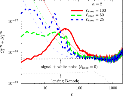
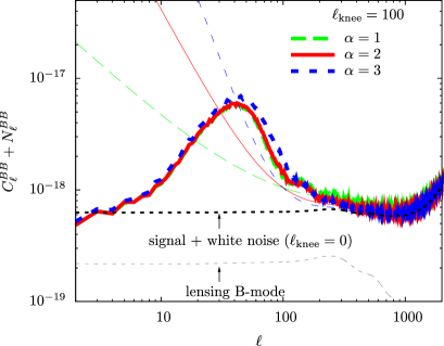
Figure 1: Left: B-mode angular power spectra after baseline subtraction (thick) compared with sums of the theoretical noise spectrum and lensing B-mode (thin), with varying $\ell_{\mathrm{knee}}=100$, $50$, $25$ but fixing $\alpha=2$ (Left). The noise level ($\Delta_{\mathrm{P}}$) is set to $6\mu$K-arcmin. We also show the case with the white noise (thick dashed) and the lensing B-mode power spectrum (thin dashed). Right: Same as the left panel but $\alpha$ is varied from $1$ to $3$ with $\ell_{\mathrm{knee}}=100$.

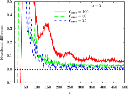
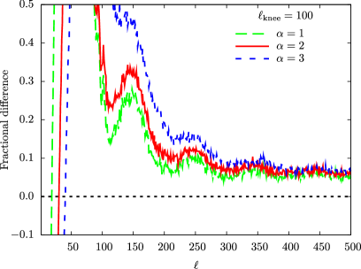
Figure 2: Same as Fig. 1 but for the fractional difference between simulated and theoretical B-mode power spectrum.

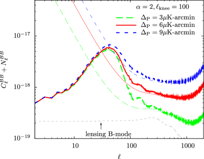
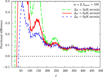
Figure 3: Left: Same as Fig. 1 but for different noise levels. Right: Same as Fig. 2 but for different noise levels.

In Fig. 1, we show B-mode power spectra obtained from the patchwork maps after baseline subtraction. The noise level ($\Delta_{\mathrm{P}}$) is set to $6\mu$K-arcmin. In the left panel, the parameter $\ell_{\mathrm{knee}}$ is varied as $100$, $50$ and $25$, while we fix $\alpha=2$. In the right panel, we fix $\ell_{\mathrm{knee}}=100$ but $\alpha$ is varied as $1$, $2$ and $3$. Conventional spherical harmonic transformation results in significant bias on the B-mode power spectrum at large scales $\ell\leq\ell_{\mathrm{knee}}$. The blowup scale of the bias depends on $\ell_{\mathrm{knee}}$. On the other hand, the dependence on $\alpha$ is not so significant.

In Fig. 2, we plot the fractional difference defined as $C^{\rm BB,sim}_{\ell}/C^{\rm BB,model}_{\ell}-1$ where $C^{\rm BB,sim}_{\ell}$ is obtained from the numerical simulations while $C^{\rm BB,model}_{\ell}$ is the sum of the theoretical noise spectrum (2.8) and lensing B-mode. The fractional difference is significant at $\ell\,\raise 2.9pt\hbox{$\scriptstyle<$}\lower 0.5pt\hbox{$\scriptscriptstyle\sim$}\;\ell_{\mathrm{knee}}$, and is still $\sim 10\%$ on scales smaller than $\ell_{\mathrm{knee}}$. In the case of Fig. 2, the lensing contributions involved in the B-mode power spectrum are $\sim 30\%$ at $\ell\,\raise 2.9pt\hbox{$\scriptstyle>$}\lower 0.5pt\hbox{$\scriptscriptstyle\sim$}\;100$ which is comparable or greater than the bias due to the baseline uncertainty. If the subpatch size becomes small, the fractional difference becomes large. These results imply that, even after the baseline subtraction, residual incoherence between subpatches still contributes to smaller scale modes through convolution with the window function $W_{i}$ which determines the subpatch size.

In Fig. 3, we also show the case with varying the noise level $\Delta_{\mathrm{P}}$ from $9\mu$K-arcmin to $3\mu$K-arcmin. As the noise level $\Delta_{\mathrm{P}}$ decreases, the bias around $\ell\sim\ell_{\mathrm{knee}}$ increases. On the other hand, the bias at $\ell\gg\ell_{\mathrm{knee}}$ is reduced by decreasing $\Delta_{\mathrm{P}}$.

3.2 Reconstructed deflection angle

3.2.1 Quadratic lensing reconstruction

Next we consider the effect of baseline uncertainties on estimates of the deflection angle. Given lensed polarization anisotropies, $\tilde{X}_{\ell m}$ and $\tilde{Y}_{\ell m}$, the lensing effect induces the off-diagonal elements of the covariance ($\ell\not=\ell^{\prime}$ or $m\not=m^{\prime}$):

$$\langle\tilde{X}_{\ell m}\tilde{Y}_{\ell^{\prime}m^{\prime}}\rangle_{\mathrm{CMB}} =\sum_{L,M}\begin{pmatrix}\ell&\ell^{\prime}&L\\ m&m^{\prime}&M\end{pmatrix}f^{\rm XY}_{\ell\ell^{\prime}L}\phi^{*}_{LM}\,,$$ (3.1)

where $\langle\cdots\rangle_{\mathrm{CMB}}$ denotes the ensemble average over the primary CMB anisotropies with a fixed realization of the lensing potential, and we ignore the higher-order terms of the lensing fields, $\mathcal{O}(\phi^{2})$. For EE and EB, the weight function $f_{\ell\ell^{\prime}L}^{\rm XY}$ in Eq. (3.1) is given by [22]

$$f^{\rm EE}_{\ell\ell^{\prime}L} =\mathcal{S}^{(+)}_{\ell\ell^{\prime}L}C^{\rm EE}_{\ell^{\prime}}+\mathcal{S}^{(+)}_{\ell^{\prime}\ell L}C^{\rm EE}_{\ell}\,,$$ (3.2)

$$f^{\rm EB}_{\ell\ell^{\prime}L} ={\rm i}\hskip 0.50003pt[\mathcal{S}^{(-)}_{\ell\ell^{\prime}L}C^{\rm BB}_{\ell^{\prime}}+\mathcal{S}^{(-)}_{\ell^{\prime}\ell L}C^{\rm EE}_{\ell}]\,.$$ (3.3)

Here $C^{\rm EE}_{\ell}$ and $C^{\rm BB}_{\ell}$ are the primary E and B-mode power spectrum, respectively. With a quadratic combination of observed polarization anisotropies, $\widehat{X}$ and $\widehat{Y}$, Eq. (3.1) leads to the lensing estimators as (e.g., [22]),

$$[\widehat{\phi}^{\rm XY}_{LM}]^{*}=A^{\rm XY}_{L}\sum_{\ell\ell^{\prime}}\sum_{mm^{\prime}}\begin{pmatrix}\ell&\ell^{\prime}&L\\ m&m^{\prime}&M\end{pmatrix}g^{\rm XY}_{\ell\ell^{\prime}L}\widehat{X}_{\ell m}\widehat{Y}_{\ell^{\prime}m^{\prime}}\,.$$ (3.4)

Here the quantity $g^{\rm XY}_{\ell\ell^{\prime}L}$ and (diagonal) normalization $A^{\rm XY}_{L}$ are given by

$$g^{\rm XY}_{\ell\ell^{\prime}L} =\frac{[f^{\rm XY}_{\ell\ell^{\prime}L}]^{*}}{\Delta^{\rm XY}\widehat{C}^{\rm XX}_{\ell}\widehat{C}^{\rm YY}_{\ell^{\prime}}}$$ (3.5)

$$A^{\rm XY}_{L} =\left\{\frac{1}{2L+1}\sum_{\ell\ell^{\prime}}f^{\rm XY}_{\ell\ell^{\prime}L}g^{\rm XY}_{\ell\ell^{\prime}L}\right\}^{-1}\,,$$ (3.6)

where $\Delta^{\rm EE}=2$, $\Delta^{\rm EB}=1$, and $\widehat{C}^{\rm XX}_{\ell}$ ($\widehat{C}^{\rm YY}_{\ell}$) is the observed power spectrum. The lensing reconstruction is then performed using the optimal combination of the EE and EB quadratic estimators:

$$\widehat{\phi}_{LM}=A_{L}\left(\frac{1}{A_{L}^{\rm EE}}\widehat{\phi}_{LM}^{\rm EE}+\frac{1}{A_{L}^{\rm EB}}\widehat{\phi}_{LM}^{\rm EB}\right)\,,$$ (3.7)

with $A_{L}^{-1}\equiv(A_{L}^{\rm EE})^{-1}+(A_{L}^{\rm EB})^{-1}$. Throughout this paper, to mitigate $\phi^{4}$-order bias [23], the lensed power spectrum ($\widetilde{C}^{\rm EE}_{\ell}$ and $\widetilde{C}^{\rm BB}_{\ell}$) is used in Eq. (3.1) rather than the primary one [24, 25]. For EB-quadratic estimator, we ignore the B-mode power spectrum in the weight function since it affects negligible contributions to the lensing estimator [22]. Note that other non-lensing anisotropies such as the residual contamination of baseline uncertainty at each subpatch can also generate the off-diagonal elements, and lead to bias on estimating the lensing potential as shown Sec. 3.2.2.

3.2.2 Effect of baseline uncertainties on lensing observables

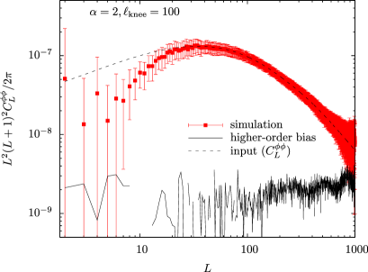
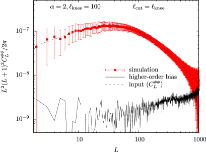
Figure 4: Left: Angular power spectrum of the lensing potential estimated from the patchwork maps with $\alpha=2$ and $\ell_{\mathrm{knee}}=100$ (red points). The noise level ($\Delta_{\mathrm{P}}$) is set to $6\mu$K-arcmin. The error bars show the variance of $C_{\ell}^{\phi\phi}$ evaluated from $100$ realizations of our simulated maps. In the lensing reconstruction, we use the E and B-mode multipoles at $2\leq\ell\leq 2000$. We also show the higher-order biases estimated from numerical simulations with $6\mu$K-arcmin and $4$ arcmin instrumental noise (solid). Right: Same as the left panel, but the E and B-modes at $\ell<\ell_{\mathrm{knee}}$ are not used in the reconstruction.

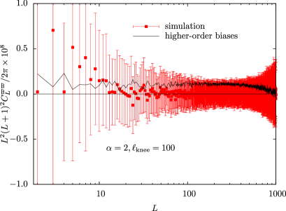
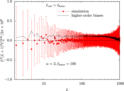
Figure 5: Same as Fig. 4 but for curl mode.

Let us discuss the effect of the baseline uncertainties on the estimation of the lensing power spectrum. From the lensing potential estimator (3.7), the lensing power spectrum is estimated through (see e.g. [9, 12])

$$\widehat{C}^{\phi\phi}_{L}=\frac{1}{2L+1}\sum_{M=-L}^{L}|\widehat{\phi}_{LM}|^{2}-\widehat{N}^{(0)}_{L}-N_{L}^{(1)}\,.$$ (3.8)

Here the quantity $\widehat{N}_{L}^{(0)}$, the so-called Gaussian bias, denotes a correction for the disconnected part of the four-point correlations, and, in this paper, we simply estimate the Gaussian bias term as $\widehat{N}_{L}^{(0)}=A_{L}$ instead of the realization dependent approaches ([26, 23, 27, 14]). The quantity $N_{L}^{(1)}$ corrects for the bias terms arising from the secondary contractions of the lensing trispectrum [28], usually referred to as N1-bias. In this paper, we estimate the N1-bias from simulated maps in which the noise is assumed to have a white spectrum [25].

In Fig. 4, we show the angular power spectrum of the lensing potential obtained from the patchwork maps in the case with $\alpha=2$ and $\ell_{\mathrm{knee}}=100$. The noise level ($\Delta_{\mathrm{P}}$) is set to $6\mu$K-arcmin. In the left panel, we perform the lensing reconstruction using CMB multipoles at $2\leq\ell\leq 2000$. If we naively use the B-mode at all scales in estimating the lensing potential ($2\leq\ell\leq 2000$), the power spectrum of the lensing estimator is biased on large scales ($L\,\,\raise 2.9pt\hbox{$\scriptstyle<$}\lower 0.5pt\hbox{$\scriptscriptstyle\sim$}\;20$). On the other hand, in the right panel, we show the same plot but the minimum multipoles of the E and B-modes used for the reconstruction $\ell_{\mathrm{cut}}$ are set to $\ell_{\mathrm{knee}}$. We find that the condition, $\ell_{\mathrm{cut}}=\ell_{\mathrm{knee}}$, would be enough to recover the lensing power spectrum. We also checked other cases of $\alpha$, $\ell_{\mathrm{knee}}$ and $\Delta_{\mathrm{P}}$, and find that $\ell_{\mathrm{cut}}=\ell_{\mathrm{knee}}$ is enough to reproduce the lensing power spectrum. This implies that, even if the B-mode power spectrum is biased due to the residual baseline uncertainty, the reconstructed lensing potential would be not so biased. This is because the bias on the B-mode power spectrum appeared in Fig. 2 is mostly absorbed into the observed power spectrum involved in $g_{\ell\ell^{\prime}L}^{\rm XY}$ (see (3.5)).

Next we consider the curl mode of the deflection angle defined in Eq. (2.2). In the future CMB lensing analysis, not only the lensing potential (i.e. gradient mode) but also the curl mode would become important to probe cosmological sources of the non-scalar metric perturbations such as primordial gravitational waves and cosmic strings (see e.g. [29]), and/or as a cross check of the lensing potential reconstruction [9]. In Fig. 5, to see whether the curl mode is consistent with zero, we show the reconstructed curl-mode power spectrum, in which we estimate the curl mode $\varpi$ following full-sky formula of Ref. [19]. Compared with the lensing potential, the curl mode is not so biased even if $\ell_{\mathrm{cut}}=2$. Note that the power spectrum of the curl mode estimator also has the higher-order biases even in the absence of the curl mode sources, and the contributions of those terms in a temperature-based reconstruction are evaluated in Refs. [30, 31]. As shown in Fig. 5, even in the polarization-based reconstruction, the higher-order biases on the curl mode would also have non-negligible contributions.

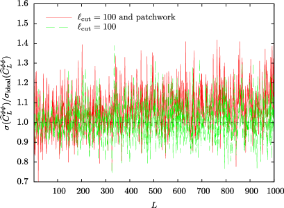
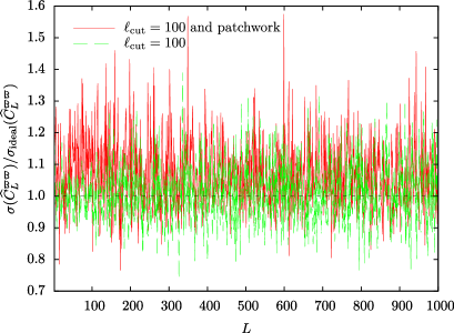
Figure 6: The variance of the gradient (left) and curl-mode (right) power spectrum estimators obtained from the patchwork maps ($\ell_{\mathrm{knee}}=100$ and $\alpha=2$) with $\ell_{\mathrm{cut}}=100$ (red) or that from coherent maps where $6\mu$K-arcmin noise is uniformly distributed but we apply $\ell_{\mathrm{cut}}=100$ to the lensing reconstruction (green). For both cases, we divide the variance by that from the coherent maps without restriction of the Fourier modes in the lensing reconstruction.

In Fig. 6, we show the variance of the power spectrum estimator for the gradient and curl mode obtained from the patchwork maps ($\ell_{\mathrm{knee}}=100$ and $\alpha=2$) with $\ell_{\mathrm{cut}}=100$ or that from coherent maps where $6\mu$K-arcmin noise is uniformly distributed but we apply $\ell_{\mathrm{cut}}=100$ to the lensing reconstruction. For both cases, we divide the variance by that from the coherent maps without restriction of the Fourier modes in the lensing reconstruction. In our case, there are two effects which affect the variance; the restriction of the Fourier modes in the lensing reconstruction, and the noisy reconstruction due to the leakage of large scale $1/f$ noise to small scales through the convolution of the subpatch window function (see Fig. 2). The results imply that the former effect is negligible if $\ell_{\mathrm{cut}}=100$. On the other hand, for gradient mode, the variance from patchwork map is increased at smaller scales (i.e., the mean of the curve for the patchwork case tends to deviate from unity at smaller scales) where the cosmic variance of the lensing potential becomes negligible. Since we do not include curl mode signal, the variance for curl mode is affected by the latter effect at almost all scales. The increase of the variance is, however, only $\sim 10\%$ even at noise dominated scales.

4 Cosmological applications of lensing observables from patchwork map

In this section, we discuss cosmological applications of the reconstructed lensing potential from the patchwork of polarization maps. In the following analysis, we cross-correlate the reconstructed potential with (coherent) full-sky CMB temperature and polarization maps. We assume that the full-sky temperature map is obtained from the PLANCK experiment. Since our original motivation is to measure lensing signals in the CMB anisotropies economically, making the full-sky polarization map by a small-size satellite is complementary to our patchwork scheme. Taking account of this point, we assume that the full-sky polarization map is measured by LiteBIRD which is a recently proposed small-size satellite observation with sensitivity high enough to measure the large scale lensing B-modes . For the simulations of such joint analysis, we additionally prepare $100$ realizations of the polarization (temperature) map in which the LiteBIRD (PLANCK) noise is generated as a Gaussian random field and then added to the polarization (temperature) map. The relevant noise level and beam size to LiteBIRD are $2\mu$K-arcmin and $30$ arcminutes FWHM, respectively [33], while the PLANCK noise level is computed according to Ref. [34].

4.1 Temperature-lensing and E-mode-lensing cross-correlations

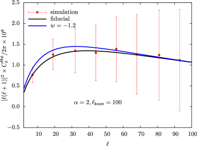
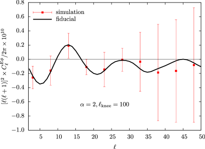
Figure 7: Temperature-lensing (left) and E-mode-lensing (right) cross-power spectrum from numerical simulations compared with the input power spectrum. In the simulations, PLANCK and LiteBIRD noises are added to the temperature and E-mode polarization, respectively. The noise level of the patchwork polarization map is set to $6\mu$K-arcmin. The error bar is computed from $100$ realizations of the numerical simulations. In the left panel, we also show the case with varying the dark-energy equation-of-state parameter $w=-1.2$ for comparison.

Since the reconstructed lensing potential is unbiased even at the largest scales, we can measure cross-power spectrum between the lensing potential and CMB temperature or E-mode polarization anisotropies which have large amplitudes on large scales ($\ell\,\raise 2.9pt\hbox{$\scriptstyle<$}\lower 0.5pt\hbox{$\scriptscriptstyle\sim$}\;100$). The galaxy-lensing cross-power spectrum would be also useful as a probe of the primordial non-Gaussianity. The gravitational potentials from the large-scale structure produces both the lensing effect and the temperature anisotropies, and the temperature-lensing cross-correlation would be a probe of the properties of the dark energy [2, 3]. The E-mode from the reionization also correlates with the deflection angle, producing E$\phi$ cross-power spectrum on large scales [24]. To show the cross-power spectra, we first define the averaging factor of the power spectrum at each bin as

$$\widehat{A}^{X\phi}_{b}\equiv(\sigma^{X\phi}_{b})^{2}\sum_{\ell=\ell^{b}_{\mathrm{min}}}^{\ell^{b}_{\mathrm{max}}}\mathscr{B}^{X\phi}_{\ell}\frac{\widehat{C}^{X\phi}_{\ell}}{C^{X\phi}_{\ell}}\,,$$ (4.1)

where the subscript $X$ is $\Theta/E$, the quantities $C^{X\phi}_{\ell}$ and $\widehat{C}^{X\phi}_{\ell}$ are the input and simulated cross-power spectrum, respectively. The multipoles $\ell^{b}_{\mathrm{min}}$ and $\ell^{b}_{\mathrm{max}}$ are the minimum and maximum multipole of the $b$-th bin, and the binning function and the variance of $\widehat{A}^{X\phi}_{b}$ at the $b$-th bin are given by

$$\mathscr{B}^{X\phi}_{\ell}=\frac{(2\ell+1)\,(C_{\ell}^{X\phi})^{2}}{(C^{\rm X\phi}_{\ell})^{2}+(C^{\rm XX}_{\ell}+\mathcal{N}_{\ell})(C^{\phi\phi}_{\ell}+A_{\ell})}\,,\qquad\sigma^{X\phi}_{b}=\left\{\sum_{\ell}\mathscr{B}^{X\phi}_{\ell}\right\}^{-1/2}\,,$$ (4.2)

with $\mathcal{N}$ denoting the PLANCK (LiteBIRD) instrumental noise if $X=\Theta$ ($E$). Then we obtain the binned power spectrum at $b$-th bin as $\widehat{C}^{X\phi}_{b}=\widehat{A}^{X\phi}_{b}C^{X\phi}_{\ell_{\mathrm{b}}}$ where $\ell_{\mathrm{b}}=(\ell^{b}_{\mathrm{min}}+\ell^{b}_{\mathrm{max}})/2$.

In Fig. 7, as a demonstration, we show the power spectra of temperature-lensing and E-mode-lensing cross-correlation. In computing the binned power spectrum, the multipole range between $\ell=2$ and $100$ is divided into $8$ bins for $\widehat{C}_{b}^{\Theta\phi}$ and $20$ bins for $\widehat{C}_{b}^{E\phi}$. The lensing potential is reconstructed using the procedure described in Sec. 3. The low-$\ell$ cut ($\ell_{\mathrm{cut}}$) is set to $\ell_{\mathrm{knee}}$ and the noise level of the patchwork map is $6\mu$K-arcmin. As expected, the cross-power spectra are consistent with the input power spectra. The signal-to-noise ratio of the cross-power spectrum is estimated as $\{\sum_{b}(\sigma_{b}^{X\phi})^{-2}\}^{1/2}$. Assuming the noise level of PLANCK, the signal-to-noise ratio of the temperature-lensing cross-correlation becomes $\sim 6.9\,\sigma$. On the other hand, by cross-correlating LiteBIRD polarization map with the reconstructed $\phi$ map, the E-mode and lensing cross-power spectrum would be detected with $\sim 2.4\,\sigma$ statistical significance.

4.2 Delensing B-mode polarization

Once we obtain the lensing potential using the quadratic estimator, we can estimate the contribution of the lensing to the B-mode polarization based on Eq. (2.6). This method is important to probe non-lensing B-modes and also used to estimate the lensing potential based on maximum-likelihood approach [17]. In this paper, we follow the method described in Ref. [7]:

$$\widehat{B}^{\rm lens}_{\ell m} =-{\rm i}\hskip 0.50003pt\sum_{\ell^{\prime}m^{\prime}}\sum_{LM}\begin{pmatrix}\ell&\ell^{\prime}&L\\ m&m^{\prime}&M\end{pmatrix}\mathcal{S}^{(-)}_{\ell\ell^{\prime}L}\mathcal{W}^{E}_{\ell^{\prime}}\mathcal{W}^{\phi}_{L}(\widehat{E}_{\ell^{\prime}m^{\prime}}\widehat{\phi}_{LM})^{*}\,,$$ (4.3)

where we define the Wiener filter, $\mathcal{W}^{\phi}_{L}=C^{\phi\phi}_{L}/(C^{\phi\phi}_{L}+A_{L})$ and $\mathcal{W}^{\rm E}_{\ell}=C^{\rm EE}_{\ell}/\widehat{C}^{\rm EE}_{\ell}$ [6, 7]. The residual B-mode polarization is then estimated from [7]

$$\widehat{B}^{\rm res}_{\ell m}=\widehat{B}_{\ell m}-\widehat{B}^{\rm lens}_{\ell m}\,.$$ (4.4)

4.2.1 Residual B-mode polarization

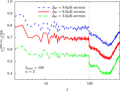
Figure 8: Residual fractions of the lensing B-modes. The residual fraction is defined as the ratio of the lensing B-mode spectrum after delensing to the original lensing B-mode spectrum. We show the cases with varying the polarization sensitivity $\Delta_{\mathrm{P}}$.

In Fig. 8, to see feasibility of the above delensing algorithm, we show residual fraction of the lensing B-mode by delensing: $C_{\ell}^{\rm BB,res}/\widetilde{C}^{\rm BB}_{\ell}$ (to clarify the delensing efficiency itself, $C_{\ell}$s in this factor do not include the noise power of LiteBIRD). By delensing, the lensing contributions in the B-mode power spectrum at $\ell<\ell_{\mathrm{knee}}$ are subtracted by approximately $30\%$ in the case that the noise level of the patchwork map is $6\mu$K-arcmin. We checked that dependence on the parameters $\alpha$ and $\ell_{\mathrm{knee}}$ is not so significant. This feature comes from the use of the EB-quadratic estimator in estimating the lensing potential (see appendix A for further explanations). The large discrepancy at $\ell\geq\ell_{\mathrm{knee}}$ would be mainly reproduced by adding correction terms described in appendix A to Eq. (2.12) of Ref.[7].

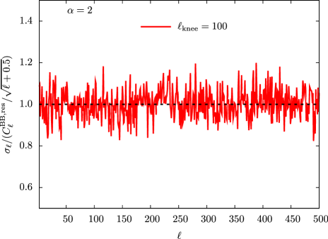
Figure 9: Variance of the residual B-mode power spectrum $\sigma_{\ell}$ obtained from $100$ realizations of the Monte Carlo simulation divided by $C_{\ell}^{\rm BB,res}/\sqrt{\ell+0.5}$, i.e., the variance obtained by assuming that the residual B-mode is Gaussian. Lensing reconstruction is performed from the patchwork maps with the noise level of $\Delta_{\mathrm{P}}=6\mu$K-arcmin and the beam size of $4$ arcmin FWHM.

In Fig. 9, we show variance of the residual B-mode power spectrum $\sigma_{\ell}$ obtained from $100$ realizations of the numerical simulations, divided by $C_{\ell}^{\rm BB,res}/\sqrt{\ell+0.5}$, i.e., the variance obtained by assuming that the residual B-mode is Gaussian. To evaluate the Gaussian variance $C_{\ell}^{\rm BB,res}/\sqrt{\ell+0.5}$, we use the residual B-mode power spectrum from the numerical simulations. The variance of the angular power spectrum does not significantly deviate from the Gaussian variance.

4.2.2 Expected constraints on primordial gravitational waves with LiteBIRD

Table 1: Expected $1\,\sigma$ constraints on $r$ of LiteBIRD observation without delensing (no delensing) and with delensing based on the joint analysis with ground-based experiments of $\Delta_{\mathrm{P}}=6\mu$K-arcmin or $3\mu$K-arcmin. We also show the case in which $90$% of the lensing components are removed ($90$% delensing) and an idealistic case where the lensing component is completely removed (LiteBIRD limit). In all cases, we use the B-mode multipoles up to $\ell=300$ where the LiteBIRD noise becomes dominant. The tensor tilt is fixed to $n_{\mathrm{t}}=-r/8$.

$r$	no delensing	$6\mu$K-arcmin	$3\mu$K-arcmin	$90$% delensing	LiteBIRD limit
$0.2$	$2.3\times 10^{-3}$	$2.2\times 10^{-3}$	$2.1\times 10^{-3}$	$1.7\times 10^{-3}$	$1.6\times 10^{-3}$
$0.02$	$4.8\times 10^{-4}$	$4.1\times 10^{-4}$	$3.8\times 10^{-4}$	$2.7\times 10^{-4}$	$2.4\times 10^{-4}$
$0.002$	$2.3\times 10^{-4}$	$1.9\times 10^{-4}$	$1.6\times 10^{-4}$	$8.7\times 10^{-5}$	$6.8\times 10^{-5}$

Table 2: Same as Table 1, but for marginalizing the tensor tilt $n_{\mathrm{t}}$. Note that the fiducial values are $r=0.2$ and $n_{\mathrm{t}}=-r/8=-0.025$.

	no delensing	$6\mu$K-arcmin	$3\mu$K-arcmin	$90$% delensing	LiteBIRD limit
$\sigma(r)$	0.0095	0.0087	0.0084	0.0072	0.0068
$\sigma(n_{\mathrm{t}})$	0.028	0.025	0.024	0.019	0.018

As an example of non-lensing B-mode probes, let us discuss the expected constraints on the amplitude and shape of the spectrum of primordial gravitational waves using a joint delensing analysis of LiteBIRD and ground-based CMB experiments. The polarization map “to be delensed” is provided by LiteBIRD and the lensing pontential map is reconstructed from the patchrork polarization map measured by ground-based experiments. Since satellite missions usually have the advantage of relatively low noise level, such joint analysis would make good synergy.

We characterize the primordial tensor power spectrum as $P_{t}(k)=rA_{\mathrm{s}}(k/k_{0})^{n_{\mathrm{t}}}$ where $r$ is the tensor-to-scalar ratio and $n_{\mathrm{t}}$ is the tensor spectral index. $A_{\mathrm{s}}$ is the amplitude of the primordial scalar power spectrum at $k_{0}$. Here, we assume that these two parameters satisfy the consistency relation $n_{\mathrm{t}}=-r/8$. The pivot scale $k_{0}$ is set to $k=0.05$ Mpc^-1.

Before moving to discuss the expected constraints on $r$ and $n_{\mathrm{t}}$, we comment on the partial subtraction of the primary B-mode [17, 8]. The origin of the primary B-mode subtraction is the same as that of the step feature in the residual B-mode shown in the previous section (see appendix A). This subtraction would also lead to a non-trivial likelihood for the residual B-mode. For the primordial gravitational waves, however, as shown in Ref. [6], this partial subtraction can be simply evaded if we incorporate only the B-mode multipoles at $\ell\geq\ell_{\mathrm{cut}}$ into the lensing reconstruction analysis and delense the multipoes at $\ell<\ell_{\mathrm{cut}}$. Information of the lensing potential mostly comes from structure of arcminute scales and LiteBIRD’s beam size is $30$ arcminutes FWHM. In the analysis below, we assume $\ell_{\mathrm{cut}}=300$. This choice of $\ell_{\mathrm{cut}}$ simultaneously mitigates the bias in the lensing potential due to reconstruction from the patchwork map (see Sec. 3.2.2).

The expected constraints on $r$ and $n_{\mathrm{t}}$ are computed based on the Fisher matrix defined as

$$F_{ij}\equiv\sum_{\ell=2}^{\ell_{\mathrm{cut}}-1}\frac{2\ell+1}{2[C_{\ell}^{\rm BB,res}]^{2}}\dfrac{\partial C^{\rm BB,res}_{\ell}}{\partial p_{i}}\dfrac{\partial C^{\rm BB,res}_{\ell}}{\partial p_{j}}\,,$$ (4.5)

where $p_{i}=r$ or $n_{\mathrm{t}}$. For simplicity, we ignore the contributions of the Galactic foreground emission . The derivatives are evaluated by finite difference method. The residual B-mode power spectrum $C^{\rm BB,res}_{\ell}$ is obtained from our numerical simulation. The fiducial values are $r=0.2$ and $n_{\mathrm{t}}=-r/8=0.025$. The expected $1\,\sigma$ error on a parameter $p_{i}$ is computed as $\sigma(p_{i})=\sqrt{\{F^{-1}\}_{ii}}$.

Although the recent BICEP2 results show $r=0.2^{+0.07}_{-0.05}$ [36], the WMAP and PLANCK constraint on $r$ is $r\,\raise 2.9pt\hbox{$\scriptstyle<$}\lower 0.5pt\hbox{$\scriptscriptstyle\sim$}\;0.1$ [13]. There are many on-going and future experiments to show whether this discrepancy is real or not. For this reason, let us first consider the expected constraints for several values of $r$ with the tensor tilt fixed as $n_{\mathrm{t}}=-r/8$. The resultant constraints are shown in Table 1. We show the cases without delensing (no delensing), and with delensing based on the joint analysis with ground-based experiments of $\Delta_{\mathrm{P}}=6\mu$K-arcmin or $3\mu$K-arcmin. We also show the case if the lensing B-mode is removed by $90$% or perfectly removed (LiteBIRD limit).

Next we consider the case if the tensor-to-scalar ratio is confirmed as $r\sim 0.2$. In Table 2, we give the expected constraints on $r$ and $n_{\mathrm{t}}$. Without delensing, the expected error of the tensor tilt $\sigma(n_{\mathrm{t}})$ is $0.028$. Delensing using a $6\mu$K-arcmin experiment would improve the constraints on $n_{\mathrm{t}}$ by $8$%. If the delensing effifiency of $90$% is attainable, the expected error reduces to $\sigma(n_{\mathrm{t}})=0.019$.

5 Summary and Discussion

We have explored for the first time the feasibility of lensing reconstruction from the patchwork of CMB polarization maps. The B-mode power spectrum of the patchwork map contains the residual bias and its significance depends on the subpatch size but slightly on the shape parameter $\alpha$. On the other hand, the bias on the estimated lensing potential would be negligible if the B-modes at $\ell<\ell_{\mathrm{knee}}$ are removed in the lensing reconstruction. We also performed a null consistency test of curl mode and found that we must care about the N1-bias on curl mode as in the case of temperature-based reconstruction [30, 31]. Based on these analyses, we discussed cosmological applications of the reconstructed lensing potential from the patchwork map. Since the lensing potential is unbiased even at the largest scale, we would measure, for example, the temperature-lensing and E-mode-lensing cross-power spectrum. Delensing of the lensing B-mode was also considered. We investigated the efficiency of delensing and found that the reconstructed potential could be used for restoring the lensing B-modes. The variance of the residual B-mode did not significantly deviate from the Gaussian variance ($C_{\ell}^{\rm BB,res}/\sqrt{\ell+0.5}$). Our parameter forecast based on Fisher matrix analysis showed that the expected LiteBIRD constraint on $r$ was improved especially in the cases of small $r$. Specifically, the expected error of $r$ reduces by $17$% ($30$%) in the case of $r=0.002$ if we delense the polarization map measured by LiteBIRD using the lensing potential reconstructed from the patchwork map with the noise level of $6\mu$K-arcmin ($3\mu$K-arcmin). We also estimated the LiteBIRD constraint on $n_{\mathrm{t}}$ in the case of $r=0.2$ which was the value claimed by BICEP2. The constraint is improved by $8$% ($12$%) if we assume the patchwork map with the noise level of $6\mu$K-arcmin ($3\mu$K-arcmin).

We comment on the case if the subpatch size becomes larger than the case considered in this paper. In this case, we can use B-modes on larger scales for unbiased lensing reconstruction. Besides, the leakage of 1/f noise to small scales decreases, which would reduce the variance of the power spectrum estimator. For delensing LiteBIRD B-mode, on the other hand, such large subpatch size would not improve the delensing efficiency if we mitigate the delensing bias by filtering out of large scale B-modes.

In our study, to focus on the effect of the baseline uncertainty on the lensing reconstruction, we used some simplifications and assumptions on the patchwork map. For example, we assumed that the map of each subpatch was measured through isotropic sky scanning. In actual situations, anisotropic sky scanning make anisotropic deficits in Fourier space. There are also other practical issues associated with this reconstruction procedure such as offsets of subpatch locations and mismatches in relative gain between subpatches. We assumed our patchwork map covered the whole sky. The finite survey area and point source mask would also be sources of systematic errors in lensing reconstruction. In our analysis, we assumed experiments which were originally designed to make a patchwork map of CMB polarization. If we consider more general case where a patchwork map contains subpatches observed by independent experiments with different experimental specifications, there would be several possible systematics such as different beam, noise levels and window functions charactering each subpatch. We checked that the “variance” of the residual B-mode power spectrum did not so deviate from that obtained assuming the residual B-modes were Gaussian. The likelihood of the residual B-mode multipoles, however, have not been thoroughly explored. Further investigation of the above issues will be presented in our future work.

Appendix A Delensing bias

In this section, we explain the step feature in the residual B-mode power spectrum also discussed in Ref. [8] as delensing bias. In the following calculations, we discuss expression for the residual B-mode power spectrum. Note that we frequently use the orthogonality relation [38]

$$\sum_{m_{1}m_{2}}\begin{pmatrix}\ell_{1}&\ell_{2}&\ell_{3}\\ m_{1}&m_{2}&m_{3}\end{pmatrix}\begin{pmatrix}\ell_{1}&\ell_{2}&\ell^{\prime}_{3}\\ m_{1}&m_{2}&m_{3}^{\prime}\end{pmatrix}=\frac{\delta_{\ell_{3}\ell_{3}^{\prime}}\delta_{m_{3}m_{3}^{\prime}}}{2\ell_{3}+1}\,,$$ (A.1)

and the symmetric property of the Wigner 3-j symbols [38]:

$$\begin{pmatrix}\ell_{1}&\ell_{2}&\ell_{3}\\ m_{1}&m_{2}&m_{3}\end{pmatrix} =\begin{pmatrix}\ell_{2}&\ell_{3}&\ell_{1}\\ m_{2}&m_{3}&m_{1}\end{pmatrix}\,,$$

$$\begin{pmatrix}\ell_{1}&\ell_{2}&\ell_{3}\\ m_{1}&m_{2}&m_{3}\end{pmatrix} =(-1)^{\ell_{1}+\ell_{2}+\ell_{3}}\begin{pmatrix}\ell_{2}&\ell_{1}&\ell_{3}\\ m_{2}&m_{1}&m_{3}\end{pmatrix}\,.$$ (A.2)

A.1 Lensing B-mode estimator

Let us consider if we use the EB-estimator for the lensing reconstruction:

$$[\widehat{\phi}^{\rm EB}_{LM}]^{*} =A^{\rm EB}_{L}\sum_{\ell\ell^{\prime}mm^{\prime}}\begin{pmatrix}\ell&\ell^{\prime}&L\\ m&m^{\prime}&M\end{pmatrix}(g^{\rm EB}_{\ell^{\prime}\ell L})^{*}\widehat{B}_{\ell m}\widehat{E}_{\ell^{\prime}m^{\prime}}\,,$$ (A.3)

where $g^{\rm EB}_{\ell^{\prime}\ell L}=-{\rm i}\hskip 0.50003pt\mathcal{S}^{(-)}_{\ell\ell^{\prime}L}\mathcal{W}^{E}_{\ell^{\prime}}/\widehat{C}^{\rm BB}_{\ell}$. Using the expression of the EB-estimator (A.3), the lensing B-mode estimator becomes

$$\widehat{B}^{\rm lens}_{\ell m} =\sum_{L\ell^{\prime}}\mathcal{W}^{\phi}_{L}A^{\rm EB}_{L}\frac{(f^{\rm EB}_{\ell^{\prime}\ell L})^{*}}{\widehat{C}^{\rm EE,LB}_{\ell^{\prime}}}\sum_{Mm^{\prime}}\begin{pmatrix}\ell&\ell^{\prime}&L\\ m&m^{\prime}&M\end{pmatrix}$$

$$\qquad\times\sum_{\ell_{1}\ell^{\prime}_{1}}\sum_{m_{1}m^{\prime}_{1}}\begin{pmatrix}\ell_{1}&\ell^{\prime}_{1}&L\\ m_{1}&m^{\prime}_{1}&M\end{pmatrix}(g^{\rm EB}_{\ell^{\prime}_{1}\ell_{1}L})^{*}(\widehat{E}^{\rm LB}_{\ell^{\prime}m^{\prime}})^{*}\widehat{B}_{\ell_{1}m_{1}}\widehat{E}_{\ell^{\prime}_{1}m^{\prime}_{1}}\,,$$ (A.4)

where $\widehat{E}^{\rm LB}_{\ell m}$ is the E-mode of LiteBIRD observation, and $\widehat{C}^{\rm EE,LB}_{\ell}$ is the LiteBIRD E-mode angular power spectrum. We first consider the following term involved in the bispectrum, which is obtained by taking ensemble average over E-mode polarization:

$$(\widehat{E}^{\rm LB}_{\ell^{\prime}m^{\prime}})^{*}\widehat{B}_{\ell_{1}m_{1}}\widehat{E}_{\ell^{\prime}_{1}m^{\prime}_{1}} \ni\delta_{\ell^{\prime}\ell^{\prime}_{1}}\delta_{m^{\prime}m^{\prime}_{1}}\widetilde{C}^{\rm EE}_{\ell^{\prime}}\widehat{B}_{\ell_{1}m_{1}}\,.$$ (A.5)

Substituting the first term in the r.h.s. of the above relation into Eq. (A.4), we obtain

$$\widehat{B}^{\rm lens}_{\ell m} \ni\sum_{\ell_{1}m_{1}}\sum_{L\ell^{\prime}}\mathcal{W}^{\rm E,LB}_{\ell^{\prime}}\mathcal{W}_{L}^{\phi}A^{\rm EB}_{L}\sum_{Mm^{\prime}}\begin{pmatrix}\ell&\ell^{\prime}&L\\ m&m^{\prime}&M\end{pmatrix}\begin{pmatrix}\ell_{1}&\ell^{\prime}&L\\ m_{1}&m^{\prime}&M\end{pmatrix}(f^{\rm EB}_{\ell^{\prime}\ell L}g^{\rm EB}_{\ell^{\prime}\ell L})^{*}\widehat{B}_{\ell_{1}m_{1}}$$

$$=\widehat{B}_{\ell m}\sum_{\ell_{1}m_{1}}\frac{\delta_{\ell\ell_{1}}\delta_{mm_{1}}}{2\ell+1}\sum_{L\ell^{\prime}}\mathcal{W}^{\rm E,LB}_{\ell^{\prime}}\mathcal{W}_{L}^{\phi}A^{\rm EB}_{L}(f^{\rm EB}_{\ell^{\prime}\ell L}g^{\rm EB}_{\ell^{\prime}\ell L})^{*}$$

$$=\widehat{B}_{\ell m}\frac{1}{\widehat{C}_{\ell}^{\rm BB}}\sum_{\ell_{1}m_{1}}\frac{\delta_{\ell\ell_{1}}\delta_{mm_{1}}}{2\ell+1}\sum_{L\ell^{\prime}}(\mathcal{S}^{(-)}_{\ell\ell^{\prime}L})^{2}[\mathcal{W}^{\rm E,LB}_{\ell^{\prime}}\mathcal{W}^{\rm E}_{\ell^{\prime}}C^{\rm EE}_{\ell^{\prime}}][\mathcal{W}_{L}^{\phi}A^{\rm EB}_{L}]$$

$$\equiv\mathcal{D}_{\ell}\widehat{B}_{\ell m}\,,$$ (A.6)

where we define $\mathcal{W}^{\rm E,LB}_{\ell}=C^{\rm EE}_{\ell}/\widehat{C}^{\rm EE,LB}_{\ell}$ and

$$\mathcal{D}_{\ell}\equiv\frac{1}{\widehat{C}_{\ell}^{\rm BB}}\sum_{\ell_{1}m_{1}}\frac{\delta_{\ell\ell_{1}}\delta_{mm_{1}}}{2\ell+1}\sum_{L\ell^{\prime}}(\mathcal{S}^{(-)}_{\ell\ell^{\prime}L})^{2}[\mathcal{W}^{\rm E,LB}_{\ell^{\prime}}\mathcal{W}^{\rm E}_{\ell^{\prime}}C^{\rm EE}_{\ell^{\prime}}][\mathcal{W}_{L}^{\phi}A^{\rm EB}_{L}]\,.$$ (A.7)

Note that, if we do not use the B-modes at $\ell<\ell_{\mathrm{min}}$ in the lensing reconstruction, the quantity (A.6) becomes zero at $\ell<\ell_{\mathrm{min}}$. This leads to the discontinuity in the residual B-mode spectrum. In actual situations, the primary B-mode is involved in $\widehat{B}_{\ell m}$, which causes the partial subtraction of primary B-mode signal as pointed out in Ref. [8].

On the other hand, a term in which the correlation between $E^{\rm LB}$ and $\widehat{\phi}$ is ignored is given by

$$\widehat{B}^{\rm lens}_{\ell m} \ni\sum_{L\ell^{\prime}}\mathcal{W}^{\phi}_{L}\frac{(f^{\rm EB}_{\ell^{\prime}\ell L})^{*}}{\widehat{C}^{\rm EE,LB}_{\ell^{\prime}}}\sum_{Mm^{\prime}}\begin{pmatrix}\ell&\ell^{\prime}&L\\ m&m^{\prime}&M\end{pmatrix}[(\widehat{E}^{\rm LB}_{\ell^{\prime}m^{\prime}}\widehat{\phi}_{LM}^{\rm EB})^{*}]_{\mathrm{d}}\equiv\widetilde{B}^{\rm W}_{\ell m}\,.$$ (A.8)

Combining the above equation and Eq. (A.6), we obtain

$$\widehat{B}^{\rm lens}_{\ell m}\simeq\widetilde{B}^{\rm W}_{\ell m}+\mathcal{D}_{\ell}\widehat{B}_{\ell m}\,.$$ (A.9)

As shown below, the second term is required to explain the step feature in the residual B-mode power spectrum. Hereafter, we call the second term $\mathcal{D}_{\ell}\widehat{B}_{\ell m}$ as delensing bias. Note that, in the above expression, the delensing bias is vanished if we estimate the lensing potential from other experiments, e.g., surveys of cosmic infrared background, galaxy weak lensing and so on.

A.2 Residual B-mode power spectrum

Now we consider the angular power spectrum of the residual B-mode in the presence of the delensing bias:

$$\langle|\widehat{B}^{\rm res}_{\ell m}|^{2}\rangle =\langle|\widehat{B}^{\rm LB}_{\ell m}-\widetilde{B}^{\rm W}_{\ell m}-\mathcal{D}_{\ell}\widehat{B}_{\ell m}|^{2}\rangle$$

$$=\langle|\widehat{B}^{\rm LB}_{\ell m}-\widetilde{B}^{\rm W}_{\ell m}|^{2}\rangle-2\mathcal{D}_{\ell}\langle|\widehat{B}^{\rm LB}_{\ell m}(\widehat{B}_{\ell m})^{*}|\rangle+2\mathcal{D}_{\ell}\langle|\widehat{B}^{\rm W}_{\ell m}(\widehat{B}_{\ell m})^{*}|\rangle+\mathcal{D}_{\ell}^{2}\langle|\widehat{B}_{\ell m}|^{2}\rangle\,.$$ (A.10)

Here we denote the B-mode polarization observed by LiteBIRD as $\widehat{B}^{\rm LB}_{\ell m}$. As shown in the above equation, the delensing bias introduces the second, third and forth terms. Note that the delensing bias is proportional to the B-mode polarization, and correlates with the B-mode to be delensed, i.e., LiteBIRD B-mode. In other words, the delensing bias leads to a realization-dependent subtraction of the B-mode to be delensed. Denoting

$$\widetilde{C}_{\ell}^{\rm BB,W}\equiv\langle|\widetilde{B}^{\rm W}_{\ell m}|^{2}\rangle=\frac{1}{2\ell+1}\sum_{\ell^{\prime}L}(\mathcal{S}^{(-)}_{\ell\ell^{\prime}L})^{2}\mathcal{W}^{\rm E,LB}_{\ell^{\prime}}\mathcal{W}_{L}^{\phi}C^{\rm EE}_{\ell^{\prime}}C_{L}^{\phi\phi}\,,$$ (A.11)

the first term is given by [7]

$$\langle|\widehat{B}^{\rm LB}_{\ell m}-\widetilde{B}^{\rm W}_{\ell m}|^{2}\rangle =\langle|\widehat{B}^{\rm LB}_{\ell m}|^{2}\rangle-2\langle\widehat{B}^{\rm LB}_{\ell m}(\widetilde{B}^{\rm W}_{\ell m})^{*}\rangle+\langle|\widetilde{B}^{\rm W}_{\ell m}|^{2}\rangle$$

$$=\widehat{C}_{\ell}^{\rm BB,LB}-2\widetilde{C}_{\ell}^{\rm BB,W}+\widetilde{C}_{\ell}^{\rm BB,W}=\widehat{C}_{\ell}^{\rm BB,LB}-\widetilde{C}_{\ell}^{\rm BB,W}\,.$$ (A.12)

The other terms due to the presence of the delensing bias become

$$\langle|\widehat{B}^{\rm LB}_{\ell m}\widehat{B}^{*}_{\ell m}|\rangle =\widetilde{C}^{\rm BB}_{\ell}\,,$$ (A.13)

$$\langle|\widetilde{B}^{\rm W}_{\ell m}\widehat{B}^{*}_{\ell m}|\rangle =\widetilde{C}_{\ell}^{\rm BB,W}\,,$$ (A.14)

$$\langle|\widehat{B}_{\ell m}|^{2}|\rangle =\widehat{C}_{\ell}^{\rm BB}\,.$$ (A.15)

By combining the above equations, we obtain the expression for the residual B-mode power spectrum in the presence of the delensing bias as

$$C^{\rm BB,res}_{\ell} =\widehat{C}^{\rm BB,LB}_{\ell}-\widetilde{C}_{\ell}^{\rm BB,W}-2\mathcal{D}_{\ell}\widetilde{C}^{\rm BB}_{\ell}+2\mathcal{D}_{\ell}\widetilde{C}_{\ell}^{\rm BB,W}+\mathcal{D}_{\ell}^{2}\widehat{C}_{\ell}^{\rm BB}\,.$$ (A.16)

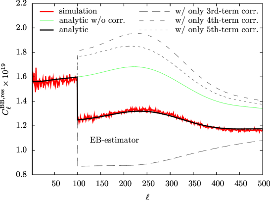
Figure 10: The residual B-mode power spectrum obtained from $100$ realizations of numerical simulation (red solid) compared with analytic expressions given in Ref. [7] (analytic w/o corr.) and Eq. (A.16) (analytic). Note that, to match the setup applied to Fig.8, we assume $r=0$ and the LiteBIRD instrumental noise in B-mode is removed. To show significance of the correction terms, we also show power spectra using only $2\mathcal{D}_{\ell}\widetilde{C}^{\rm BB}_{\ell}$ (w/ only 3rd-term corr.), $2\mathcal{D}_{\ell}\widetilde{C}_{\ell}^{\rm BB,W}$ (w/ only 4th-term corr.) or $\mathcal{D}_{\ell}^{2}\widehat{C}_{\ell}^{\rm BB}$ (w/ only 5th-term corr.) as a correction of the delensing bias term in Eq. (A.16). In the numerical simulation, the lensing potential is reconstructed with the EB-quadratic estimator, and we add white noise as a random Gaussian field assuming our fiducial noise level and beam size ($\Delta_{\mathrm{P}}=6\mu$K-arcmin and $\theta=4$ arcmin).

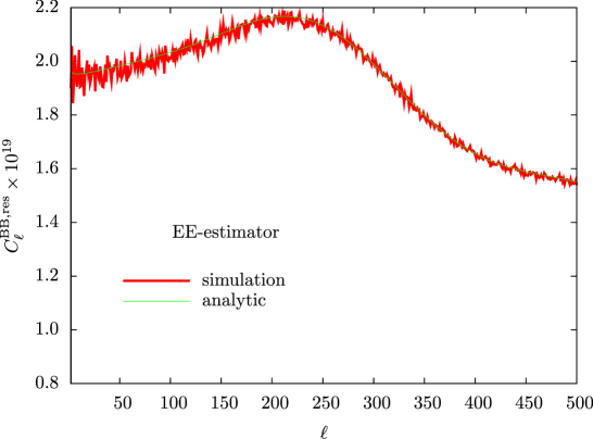
Figure 11: Same as Fig. 10 but for the case with the EE-quadratic estimator.

In Fig. 10, we compare the theoretical power spectrum (A.16) with the residual B-mode from the numerical simulation with a white noise generated as a random Gaussian field assuming the noise level of $\Delta_{\mathrm{P}}=6\mu$K-arcmin and the beam size of $4$ arcminutes FWHM. To match the setup applied to Fig. 8, we assume $r=0$ and the LiteBIRD instrumental noise in B-mode is removed. As shown in Fig. 10, the resultant residual B-mode power spectrum is suppressed at $\ell\geq\ell_{\mathrm{cut}}$. This implies that the third term in Eq. (A.16) which comes from the correlations between the delensing bias and LiteBIRD B-mode is significant compared to other bias terms. On the other hand, in Fig. 11, we show the case with the EE quadratic estimator for the lensing reconstruction. For EE-estimator, since $\mathcal{D}_{\ell}=0$, the analytic power spectrum of Eq. (A.12) is in good agreement with the results of the numerical simulations.

References

- [1] M. Zaldarriaga and U. Seljak, Gravitational lensing effect on cosmic microwave background polarization, Phys. Rev. D 58 (1998) 023003, [astro-ph/9803150].
- [2] D. M. Goldberg and D. N. Spergel, Microwave background bispectrum. 2. A probe of the low redshift universe, Phys. Rev. D 59 (1999) 103002, [astro-ph/9811251].
- [3] U. Seljak and M. Zaldarriaga, Direct signature of evolving gravitational potential from cosmic microwave background, Phys. Rev. D 60 (1999) 043504, [astro-ph/9811123].
- [4] L. Knox and Y.-S. Song, A Limit on the detectability of the energy scale of inflation, Phys. Rev. Lett. 89 (2002) 011303, [astro-ph/0202286].
- [5] M. Kesden, A. Cooray, and M. Kamionkowski, Separation of gravitational wave and cosmic shear contributions to cosmic microwave background polarization, Phys. Rev. Lett. 89 (2002) 011304, [astro-ph/0202434].
- [6] U. Seljak and C. M. Hirata, Gravitational lensing as a contaminant of the gravity wave signal in CMB, Phys. Rev. D 69 (2004) 043005, [astro-ph/0310163].
- [7] K. M. Smith et al., Delensing CMB Polarization with External Datasets, JCAP 1206 (2012) 014, [arXiv:1010.0048].
- [8] W.-H. Teng, C.-L. Kuo, and J.-H. P. Wu, Cosmic Microwave Background Delensing Revisited: Residual Biases and a Simple Fix, arXiv:1102.5729.
- [9] PLANCK Collaboration, Planck 2013 results. XVII. Gravitational lensing by large-scale structure, arXiv:1303.5077.
- [10] D. Hanson et al., Detection of B-mode Polarization in the Cosmic Microwave Background with Data from the South Pole Telescope, Phys. Rev. Lett. 111 (2013) 141301, [arXiv:1307.5830].
- [11] POLARBEAR Collaboration, Gravitational Lensing of Cosmic Microwave Background Polarization, arXiv:1312.6646.
- [12] T. Namikawa, Cosmology from weak lensing of CMB, Prog. Theor. Exp. Phys. 2014 (2014) 06B108, [arXiv:1403.3569].
- [13] PLANCK Collaboration, Planck 2013 results. XVI. Cosmological parameters, arXiv:1303.5076.
- [14] T. Namikawa and R. Takahashi, Bias-Hardened CMB Lensing with Polarization, Mon. Not. Roy. Astron. Soc. 438 (2013) 1507, [arXiv:1209.0091].
- [15] R. Pearson, B. Sherwin, and A. Lewis, CMB lensing reconstruction using cut sky polarization maps and pure-B modes, arXiv:1403.3911.
- [16] K. Gorski et al., HEALPix - A Framework for high resolution discretization, and fast analysis of data distributed on the sphere, Astrophys. J. 622 (2005) 759–771, [astro-ph/0409513].
- [17] C. M. Hirata and U. Seljak, Reconstruction of lensing from the cosmic microwave background polarization, Phys. Rev. D 68 (2003) 083002, [astro-ph/0306354].
- [18] A. Cooray, M. Kamionkowski, and R. R. Caldwell, Cosmic shear of the microwave background: The curl diagnostic, Phys. Rev. D D71 (2005) 123527, [astro-ph/0503002].
- [19] T. Namikawa, D. Yamauchi, and A. Taruya, Full-sky lensing reconstruction of gradient and curl modes from CMB maps, JCAP 1201 (2012) 007, [arXiv:1110.1718].
- [20] W. Hu, Weak lensing of the CMB: A harmonic approach, Phys. Rev. D 62 (2000) 043007, [astro-ph/0001303].
- [21] A. Lewis, A. Challinor, and A. Lasenby, Efficient Computation of CMB anisotropies in closed FRW models, Astrophys. J. 538 (2000) 473–476, [astro-ph/9911177].
- [22] T. Okamoto and W. Hu, CMB Lensing Reconstruction on the Full Sky, Phys. Rev. D 67 (2003) 083002, [astro-ph/0301031].
- [23] D. Hanson et al., CMB temperature lensing power reconstruction, Phys. Rev. D 83 (2011) 043005, [arXiv:1008.4403].
- [24] A. Lewis, A. Challinor, and D. Hanson, The shape of the CMB lensing bispectrum, JCAP 1103 (2011) 018, [arXiv:1101.2234].
- [25] E. Anderes, Decomposing CMB lensing power with simulation, Phys. Rev. D (2013) [arXiv:1301.2576].
- [26] C. Dvorkin and K. M. Smith, Reconstructing Patchy Reionization from the Cosmic Microwave Background, Phys. Rev. D 79 (2009) 043003, [arXiv:0812.1566].
- [27] T. Namikawa, D. Hanson, and R. Takahashi, Bias-Hardened CMB Lensing, Mon. Not. Roy. Astron. Soc. 431 (2013) 609–620, [arXiv:1209.0091].
- [28] M. H. Kesden, A. Cooray, and M. Kamionkowski, Lensing reconstruction with CMB temperature and polarization, Phys. Rev. D 67 (2003) 123507, [astro-ph/0302536].
- [29] T. Namikawa, D. Yamauchi, and A. Taruya, Constraining cosmic string parameters with curl mode of CMB lensing, Phys.Rev. D88 (2013) 083525, [arXiv:1308.6068].
- [30] A. van Engelen et al., A measurement of gravitational lensing of the microwave background using South Pole Telescope data, arXiv:1202.0546.
- [31] A. Benoit-Levy et al., Full-sky CMB lensing reconstruction in presence of sky-cuts, Astron. Astrophys. 555 (2013) 10, [arXiv:1301.4145].
- [32] A. Kogut et al., The Primordial Inflation Explorer (PIXIE): A Nulling Polarimeter for Cosmic Microwave Background Observations, JCAP 1107 (2011) 025, [arXiv:1105.2044].
- [33] T. Matsumura et al., Mission design of LiteBIRD, astro-ph/1311.2847.
- [34] PLANCK Collaboration, The scientific programme, astro-ph/0604069.
- [35] N. Katayama and E. Komatsu, Simple foreground cleaning algorithm for detecting primordial B-mode polarization of the cosmic microwave background, Astrophys. J. 737 (2011) 78, [arXiv:1101.5210].
- [36] BICEP2 Collaboration, BICEP2 I: Detection of B-mode Polarization at Degree Angular Scales, arXiv:1403.3985.
- [37] A. Challinor and A. Lewis, Lensed CMB power spectra from all-sky correlation functions, Phys. Rev. D 71 (2005) 103010, [astro-ph/0502425].
- [38] D. Varshalovich, A. Moskalev, and V. Kersonskii, Quantum Theory of Angular Momentum. World Scientific, 1989.