Invariant versus classical quartet inference when evolution is heterogeneous across sites and lineages

Jesús Fernández-Sánchez¹ and Marta Casanellas^1
1Dept. Matemàtica Aplicada I, Universitat Politècnica de Catalunya

Dept. Matemàtica Aplicada I, Universitat Politècnica de Catalunya
Gran Via 585, 08023-Barcelona, Spain
E-mail: jesus.fernandez.sanchez@upc.edu, marta.casanellas@upc.edu.

Abstract

One reason why classical phylogenetic reconstruction methods fail to correctly infer the underlying topology is because they assume oversimplified models. In this paper we propose a topology reconstruction method consistent with the most general Markov model of nucleotide substitution, which can also deal with data coming from mixtures on the same topology. It is based on an idea of Eriksson on using phylogenetic invariants and provides a system of weights that can be used as input of quartet-based methods. We study its performance on real data and on a wide range of simulated 4-taxon data (both time-homogeneous and nonhomogeneous, with or without among-site rate heterogeneity, and with different branch length settings). We compare it to the classical methods of neighbor-joining (with paralinear distance), maximum likelihood (with different underlying models), and maximum parsimony. Our results show that this method is accurate and robust, has a similar performance to ML when data satisfies the assumptions of both methods, and outperforms all methods when these are based on inappropriate substitution models or when both long and short branches are present. If alignments are long enough, then it also outperforms other methods when some of its assumptions are violated.
[Keywords: phylogenetic invariants, topology reconstruction, general Markov model, heterogeneity across lineages, heterogeneity across sites, yeast]

Introduction

Classical methods of phylogenetic tree topology reconstruction are known to have limitations. For example, maximum likelihood (ML) is known to fail when data violates some of the underlying model assumptions (Swofford et al. 2001; Kück et al. 2012; Ho and Jermiin 2004); maximum parsimony (MP) is statistically inconsistent in the Felsenstein zone (Felsenstein 1978); and neighbor-joining (NJ) is subject to the choice of an unbiased distance and it is not as accurate as ML when both methods can be applied (Tateno et al. 1994). When trying to estimate distant phylogenies, neglecting heterogeneity in the substitution process across lineages (HAL from now on, as denoted in Jayaswal et al. (2014)) or heterogeneity across sites (HAS) may result in inaccurate phylogenetic estimates (see Yang and Roberts (1995); Ho and Jermiin (2004); Foster (2004); Galtier and Gouy (1998); Felsenstein (1978); Yang (1994); Fitch (1986); Stefankovic and Vigoda (2007); Kolaczkowski and Thornton (2004) among others).

Phylogenetic invariants were first introduced by Cavender and Felsenstein (1987) and Lake (1987) as a non-parametric method of phylogenetic reconstruction: they are equations satisfied by any possible joint distribution of character patterns at the leaves of a tree evolving under an evolutionary Markov model. The potential of phylogenetic invariants was the ability of dealing with more general models and of detecting the topology without estimating branch lengths or substitution parameters (see Felsenstein 2004, chapter 22). In particular, they can handle HAL better than other methods (Casanellas and Fernández-Sánchez 2007; Holland et al. 2013) and (some) could deal with HAS, as Lake’s invariants did (Lake 1987). Nevertheless, only a few phylogenetic invariants were known by that time, it was not clear how to use them (Felsenstein 2004), they seemed useless for large trees, and the approach was laid aside by the bad results obtained in simulations (Huelsenbeck 1995).

Eriksson (2005) proposed a new topology reconstruction method, ErikSVD, based on the work on invariants of Allman and Rhodes (2007). The underlying idea is that organizing the joint distribution of character patterns according to a bipartition of the set of taxa gives a bipartition matrix (5) of rank $\leq 4$ if the bipartition is induced by an edge of the tree (and otherwise, the rank is higher). This result holds for any set of DNA sequences evolving under the most general Markov model (GMM), also known as Barry Hartigan’s model (Barry and Hartigan 1987; Allman and Rhodes 2008; Jayaswal et al. 2005). This is the most general HAL model as it allows different instantaneous rate matrices and heterogeneous composition at different parts of the tree, even locally along each branch (Jayaswal et al. 2011). ErikSVD does not use phylogenetic invariants directly but computes the Frobenius distance of the bipartition matrices to the set of matrices of rank $\leq 4$. Although it is nowadays clear that phylogenetic invariants derived from rank conditions on matrices are the only relevant invariants for reconstructing the topology (Casanellas and Fernández-Sánchez 2010), the original method ErikSVD turned out not to be accurate enough to compete against standard methods (Eriksson 2005), especially in the presence of long branches and short alignments.

Here we revisit ErikSVD by correcting the target matrix: in the method Erik+2 proposed here we consider the two possible transition matrices from the states of one side of the bipartition to the other (that is, we normalize by column and row sum the bipartition matrix of ErikSVD). This correction is made to take into account that the rank of the bipartition matrix obtained from empirical distributions could be affected by the presence of long-branch attraction situations (see Appendix 1). The original ErikSVD was already statistically consistent (that is, as the empirical distribution approaches the theoretical distribution, the probability of correctly reconstructing the tree goes to one) and so is the new method (see Materials and Methods).

Erik+2 is model-based as it assumes a general Markov model of evolution (and it could also be redesigned to incorporate more restrictive Markov models or even aminoacid substitution models), but is non-parametric in the sense that it does not attempt to recover the parameters of the model. Moreover, the theoretical background of Erik+2 permits to apply it on HAS data evolved on the same tree topology under GMM (Jayaswal et al. 2014): that is, a parameter $m$ can be introduced so that Erik+2 considers the sites of the alignment to be divided into $m$ categories, each evolving on the same topology but with (possibly) different Markov substitution matrices –this is called an m-mixture (Stefankovic and Vigoda 2007). For example, discrete-gamma rates or the heterogeneous tree in (Kolaczkowski and Thornton 2004) are instances of mixtures, and ML is known to fail under these conditions even when consistent underlying homogeneous models are considered (Kück et al. 2012; Kolaczkowski and Thornton 2004). For $m$-mixtures, the rank of the bipartition matrix induced by an edge is not larger than $4m$ (e.g. Rhodes and Sullivant 2012) so that in this case we use the distance to matrices of rank $\leq 4m$.

We develop Erik+2 on 4-taxon trees and study its performance on simulated and real data. Using computer simulations we compare it to the classical methods ML, NJ, MP and to the original ErikSVD in many different scenarios. We chose quartets because they are the smallest building blocks of phylogenetic reconstruction (Ranwez and Gascuel 2001) and they are widely used as a hint of efficiency and robustness of the method under study (Huelsenbeck 1995). Erik+2 evaluates the three possible quartet topologies and returns a system of weights that can be used as input for quartet-based methods (see the Methods section).

Some of our computer simulations are generated under the general Markov process that underlies Erik+2 and some are based on themost general time-reversible (GTR) and homogeneous across lineages model (homGTR from now on). We also simulate HAS data by generating either 2-mixtures on the same topology evolving under GMM or Gamma continuously-distributed rates across sites under the homGTR model. Throughout the paper NJ has been considered with the paralinear distance, and ML computations have been based on continuous-time models (with parameters to be estimated by the method) considering homogeneity or heterogeneity across lineages and sites depending on the situation (we detail it explicitly in figure captions).

The performance of Erik+2 on real data is analyzed on the eight species of yeast studied in Rokas et al. (2003) with the concatenated alignment provided by Jayaswal et al. (2014). We investigate whether the quartets output by Erik+2 and ErikSVD support the tree $T$ of Rokas et al. (2003) or the alternative tree $T^{\prime}$ of Phillips et al. (2004), and the mixture model proposed by Jayaswal et al. (2014).

Results

We present the performance of the new method Erik+2, the original method of Eriksson (ErikSVD), and the classical methods ML, NJ and MP, on quartet reconstruction on different simulated data. Erik+2 is publicly available at the webpage
http://www.pagines.ma1.upc.edu/$\sim$casanellas/Erik+2.html.

Homogeneity across sites

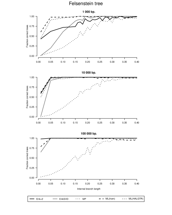
Figure 2: Percentage of correctly reconstructed topologies by Erik+2, ErikSVD, maximum likelihood ML, and maximum-parsimony MP on data generated under the general Markov model (GMM) on the tree of Figure 1.a with $a=0.05$, $b=0.75$, and varying the internal branch length $c$. Two types of ML inference have been applied here: ML(hom) estimating the most general homogeneous continuous-time model, and ML(HALGTR) estimating a HAL GTR model (due to the time of execution of this last method, we could only test it for 1 000 bp. and 10 000 bp.).

First of all we consider a tree subject to long branch attraction. On the tree of Figure 1.a we fix $a=0.05$, $b=0.75,$ and let the internal branch length $c$ vary in the range $[0.01,0.4]$ so that the tree lies in the Felsenstein zone. Alignments of lengths 1 000, 10 000 and 100 000 base pairs (bp.) were generated under GMM according to this tree. The results obtained for Erik+2, ML, MP and ErikSVD on these data are shown in Figure 2. In this figure two models underlying ML computations have been considered: the most general homogeneous continuous-time model, ML(hom) from now on, and a HAL GTR model, ML(HALGTR) henceforth. ML has a similar performance with both models. We observe that, Erik+2 is more accurate than ErikSVD in general and especially when the interior branch length is short (only for length 1 000 and $c\in(0.13,0.25)$ ErikSVD outperforms slightly Erik+2). For 1 000 sites, both versions of ML perform better than Erik+2, but when more data is available Erik+2 outperforms ML (in its both versions). Notice incidentally that the accuracy of ML or MP does not seem to increase as the length of the alignment grows, while it certainly does for ErikSVD and Erik+2.

In a more complete study, we adopted a similar approach to Huelsenbeck (1995) to test different methods. More precisely, we evaluate the methods on a tree space (see Figure 1.b) where the quartets are as in Figure 1.a with $c=a$, and the branch lengths $a$ and $b$ vary between 0 and 1.5 in steps of 0.02. For each pair $a,b$ we generated 100 alignments of a fixed length and represented in a gray scale the success of different methods in recovering the right topology (black means 100 % of success, and white 0 %). The methods Erik+2, ML, and NJ with paralinear distance have been tested according to this approach. The results for 1 000 and 10 000 bp. are shown in Figure 3 for data generated under GMM and ML estimating the most general homogeneous continuous-time model ML(hom), and in Figure 4 for data generated under homogeneous GTR model and ML estimating exactly the same model, ML(homGTR).

In Figure 3, we see that both ML(hom) and NJ have lower accuracy than Erik+2, as it was expected under data that violates the assumptions of ML and NJ. In both figures 3 and 4 we observe that, while Erik+2 and NJ drastically increase their accuracy when alignment length is multiplied by 10, ML does not significantly improve with alignment length (especially in Figure 3 when the substitution model assumed by ML is incorrect). In Figure S1 of the Appendix 2 the reader can find the performance of ErikSVD on the tree space of Figure 1.b, confirming the improvement of Erik+2 over the original method. The average success and standard deviation achieved by these methods on this tree space are shown in Table 1 (where alignment length 500 bp. is also included).

It is worth pointing out that, for alignments of 1 000 bp. evolving under homogeneous GTR model, ML(homGTR) seems to perform better than Erik+2 in the Felsenstein zone. However, for length 10 000, Erik+2 already outperforms ML(homGTR) (Fig. 4). Moreover, the global accuracy of ML(hom) drastically drops when applied to data obtained under GMM (see Fig. 3). Notice also that whereas the accuracy of NJ and ML drops when all branches are long (top right corner), the performance of Erik+2 seems less sensitive to long branches.

We have also evaluated the version of Erik+2 with 2-mixtures ($m=2$) on the same data (see Fig. S3 in Appendix 2). The accuracy obtained for alignments of 1 000 bp. is similar to that of Erik+2 with $m=1$ (the means are 0.790 and 0.803, respectively), and hence the choice $m=2$ appears as a good option when alignments are long enough and we ignore whether the data comes from mixtures or not (see also Fig. S4 in Appendix 2).

Heterogeneity across sites (HAS)

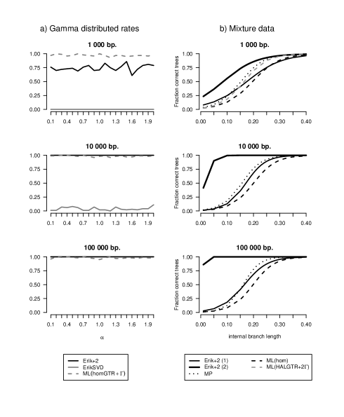
Figure 5: Percentage of correctly reconstructed topologies by different methods on alignments of lengths 1 000, 10 000 and 100 000 bp. shown from top to bottom. a) Erik+2, ErikSVD, and ML estimating the GTR model (homogeneous across lineages) with auto-discrete Gamma-rates and denoted as ML(GTR+$\Gamma$). Data simulated under (homogeneous across lineages) GTR model with continuous Gamma-rates and parameter $\alpha$ varying between 0.1 and 2 on the tree of Figure 1.a with branch lengths $a=c=0.05$ and $b=0.75$ (MP had 0% success on this data, so we do not show it). b) Data generated under GMM with 2 categories according to the test designed in (Kolaczkowski and Thornton 2004), varying the internal branch length, and recovering with Erik+2 with $m=2$, Erik+2 with $m=1$, MP, ML(hom) estimating the most general homogeneous across lineages model, and ML(HALGTR+2$\Gamma$) estimating HAL time-reversible model with 2 discrete-Gamma categories (due to the time of execution of this last method, we could only test it for 1 000 bp). The plot represents the logistic regression curve of the output of each method. In all cases, ML had to estimate all parameters.

On the same tree of Figure 1.a, we generated data under homogeneous GTR model with sites varying according to a Gamma distribution with parameter $\alpha=\beta$ in the range $(0,2]$ varying in steps of $0.1$. Small values of this parameter indicate a lot of variation across sites (Yang 1993). While this setting violates the hypotheses of the model underlying Erik+2 and ErikSVD, in this case maximum likelihood is estimating a homogeneous GTR model with rates varying according to the auto-discrete Gamma model ML(homGTR+$\Gamma$) (Yang 1994). The results appear in Figure 5.a, where we observe that Erik+2 manages to overcome the violation of its hypotheses giving 100% success already for 10 000 bp., while ErikSVD gives notably worse results. ML is more successful than Erik+2 for 1 000 bp., but both methods have a similar performance on longer alignments. On the same data we also tested MP, obtaining in all cases the incorrect tree $13|24$ (and therefore we do not represent the corresponding 0% line in the figure).

As mentioned above, one of the main features of Erik+2 is that it can deal with different categories of evolutionary rates. In order to test its accuracy on such setting, we used the approach of Kolaczkowski and Thornton (2004). We considered two categories of the same size both evolving under GMM on the tree of Figure 1.a: the first category corresponds to branch lengths $a=0.05$, $b=0.75$, while the second corresponds to $a=0.75$ and $b=0.05$. The internal branch length was set to the same value in both categories and varied from 0.01 to 0.4. In Figure 5.b) we present the performance of Erik+2 (with $m=1$ and $m=2$), MP, ML(hom), and ML estimating a HAL GTR model with discrete Gamma rates with 2 categories, ML(HALGTR+2$\Gamma$) henceforth. We included MP in this study because, as stated in Kolaczkowski and Thornton (2004), it performs better than ML estimating a single category model. This claim is confirmed by the results in our simulations with both versions of ML. It is worth pointing out that even Erik+2 with $m=1$ performs better than ML(hom) for internal branch length $\leq 0.25$, and than ML(HALGTR+2$\Gamma$) for internal branch length $\leq 0.15$. Also, notice that for length 10 000 and larger, the accuracy of Erik+2 with $m=2$ is always greater than 33%, even if the internal branch length is close to zero. This does not happen for ML, MP, which are clearly inconsistent in this setting.

Performance on real data

We considered the data provided by Jayaswal et al. (2014) with 42 337 second codon positions of 106 orthologous genes of Saccharomyces cerevisiae, S. paradoxus, S. mikatae, S. kudriavzevii, S. castellii, S. kluyveri, S. bayanus, and Candida albicans. The phylogenetic tree of these species was originally studied in Rokas et al. (2003), where a tree topology $T$ was identified with 100% bootstrap support for the concatenated alignment of these genes. This tree is widely accepted by the community but its correct inference is known to depend on the consideration of HAL (Rokas et al. 2003; Phillips et al. 2004; Jayaswal et al. 2014). For example, Phillips et al. (2004) obtain an alternative tree $T^{\prime}$ with 100% bootstrap using the method of minimum evolution, but identified the incorrect handling of compositional bias as responsible for this inconsistency. Moreover, according to Jayaswal et al. (2014) these data is best modeled by taking into account HAL plus two different rate categories and invariable sites. In our setting, this would involve three mixtures. We apply ErikSVD and Erik+2 with $m=1,2,3$ to 4-taxon subalignments and investigate the proportion of output quartets that are compatible with $T$ or $T^{\prime}$. The results displayed in Table 2 show that Erik+2 supports the tree $T$ and the model suggested by Jayaswal et al. (2014) ($m=3$), whereas ErikSVD gives more support to the alternative tree $T^{\prime}$.

Time of execution

We have compared the time of execution of the different reconstruction methods used in our simulations with 100 alignments of length 1 000 bp on a 3.2GHz processor. The results obtained show that NJ is the fastest method, 1.324s. ErikSVD and Erik+2 take 1.928s and 2.148s respectively, and MP takes 3.984s. Finally, ML is the slowest method by far because it has to infer the model parameters: using PAML software, ML(hom) and ML(homGTR) need about 10 seconds, and using bppml of Bio++ package, ML(HALGTR) and ML(HALGTR+2$\Gamma$) need about 200 minutes.

Discussion

The simulation studies show that Erik+2 is an accurate and robust topology reconstruction method on quartets, especially in situations where other methods systematically fail (compositional heterogeneity and/or rate heterogeneity across lineages, or long branch attraction). In such scenarios, Erik+2 outperforms the method of Eriksson, ErikSVD, and classical methods like MP, NJ and ML based on models that cannot accommodate these assumptions. Erik+2 is based on the most general Markov model and hence accounts for HAL data, even locally at each edge. When its assumptions are violated, for example in the presence of continuous Gamma-distributed rates among sites, we have shown that it is highly accurate if there is enough data. As observed, Erik+2 can also deal with $m$-mixtures on the same tree topology (although for quartets the limit is $m=3$). Even more, using Erik+2 with $m=2$ is probably the best option for large alignments when mixed/unmixed nature of data is unknown.

On the experiments we presented, the overall performance of ML is quite accurate if model assumptions are not violated, confirming the conclusions of Kolaczkowski and Thornton (2004); Kück et al. (2012). Also in line with these papers, we corroborate that long sequences do not improve ML performance on data that do not satisfy the hypothesis of the underlying model. Moreover, ML is by far the slowest among the methods tested here, while Erik+2 is slightly twice slower than NJ. Another drawback of ML is that, quite often, it does not converge when it is computed on the incorrect topology, which makes the comparison of likelihoods impossible. Whereas the goal of Erik+2 is to reconstruct the topology, ML is designed to estimate the parameters of the substitution matrices and, it would probably be a good choice to use first Erik+2 and then ML to estimate the parameters. In our simulation study, NJ (with paralinear distance) and MP have been the methods with least success, which is not so surprising if one takes into account that they are also the less adaptable to general data.

We have only developed Erik+2 for quartets with the aim of validating it as a successful method, and it is still a work in progress to further develop it for larger number of taxa. Using Erik+2 to evaluate the confidence of particular bipartitions of large sets of taxa is already a viable option, and in this case one can deal with a larger number $m$ of categories (the maximum $m$ allowed depends on the size of the subsets $A$, $B$ of taxa involved in the bipartition: $4^{min\{|A|,|B|\}-1}-1$). We have also started testing its weights as input of weighted quartet-based methods with high success (unpublished). In particular, it outperforms global NJ, which makes Erik+2 a potential input method for quartet-based methods (St. John et al. 2003).

Materials and Methods

ErikSVD and Erik+2 methods

Erik+2 arises as a variation of the method described by Eriksson (2005) by normalizing certain bipartition matrices obtained from an alignment of nucleotide sequences. As in the original method, the information contained in the alignment is recorded as a vector $\tilde{p}$ whose coordinates are the observed relative frequencies of possible patterns at the leaves. In the case of an alignment of four taxa 1,2,3,4, each possible (trivalent) topology is determined by a bipartition of thetaxa: $12|34$, $13|24$ or $14|23$. For each bipartition $A|B$, a matrix $M_{A\mid B}(\tilde{p})$ is considered by rearranging the coordinates of $\tilde{p}$ according to it, so that the rows of the matrix $M_{12|34}(\tilde{p})$ are indexed by all possible observations $(x_{1},x_{2})$ at the leaves $1,2$, and similarly for columns and observations $(x_{3},x_{4})$ at the leaves $3,4$. For example, the $(AG,CT)$-entry of $M_{12|34}(\tilde{p})$ is the relative frequency $\tilde{p}_{AGCT}$ of the pattern $AGCT$ in the alignment. The same entry in $M_{13|24}(\tilde{p})$ corresponds to the relative frequency $\tilde{p}_{ACGT}$ of $ACGT$.

$$M_{12\mid 34}(\tilde{p})=\left(\begin{array}[]{ccccc}\tilde{p}_{AAAA}&\tilde{p}_{AAAC}&\tilde{p}_{AAAG}&\ldots&\tilde{p}_{AATT}\\ \tilde{p}_{ACAA}&\tilde{p}_{ACAC}&\tilde{p}_{ACAG}&\ldots&\tilde{p}_{ACTT}\\ \tilde{p}_{AGAA}&\tilde{p}_{AGAC}&\tilde{p}_{AGAG}&\ldots&\tilde{p}_{AGTT}\\ \ldots&\ldots&\ldots&&\ldots\\ \end{array}\right)$$ (5)

Assume that the coordinates of $\tilde{p}$ are the empirical estimates of the theoretical joint distribution $p$ at the leaves of a tree $T$ evolving under GMM, say $T=12|34$. Then the key point is Theorem 19.5 of Eriksson (2005) (see Casanellas and Fernández-Sánchez (2010) for a complete proof) that claims that the rank of $M_{A|B}(p)$ is $4$ if $A|B=12|34$, and $4^{2}$ otherwise (if the substitution matrices that generated $p$ were general enough). Eriksson’s idea is to compute the Frobenius distance (that is, the euclidean distance if we view the matrices as elements in $\mathbb{R}^{4^{2}\times 4^{2}}$, Demmel 1997) $\mathrm{d_{4}}$ of the three matrices $M_{12|34}(\tilde{p})$, $M_{13|24}(\tilde{p})$ and $M_{14|23}(\tilde{p})$ to the space of matrices of rank $\leq 4$. In this manner, one derives which of the three matrices is closer to having rank $\leq 4$. The Frobenius distance of a matrix $A$ to $k$-rank matrices, $\mathrm{d_{k}}(A)$, is easily computed in terms of the singular values of $A$ (Eckart and Young 1936).

The main motivation for the variation introduced in Erik+2 arises from the observation that the presence of short branches may seriously affect this distance when its computed from short alignments. For example, taking the tree of Figure 1.a with small $a$ and large $b$ (a tree corresponding to the so-called Felsenstein’s zone), the distance of $M_{13|24}(\tilde{p})$ to 4-rank matrices is smaller than that of $M_{12|34}(\tilde{p})$ (see Appendix 1 for an example). The reason is that a small $a$ implies that the probability of observing the same nucleotide at leaves 2 and 4 is high, so columns in $M_{13|24}(\tilde{p})$ indexed by $AA$, $CC$, $GG$, or $TT$ capture most of the non-zero entries in the matrix, while other columns may only have few nonzero entries. This makes the matrix to be close to a rank $\leq 4$ matrix, even if $13|24$ is not the correct topology. By dividing any non-zero column by the sum of its entries, we make all the non-zero columns to have the same weight. As the same situation may occur with rows, we also need to correct the matrix by row sums. In this way, each matrix $M_{A|B}(\tilde{p})$ gives rise to a pair of transition matrices $M_{A\rightarrow B}(\tilde{p})$ and $M_{A\leftarrow B}(\tilde{p})$, obtained by column and row sum correction, respectively:

$$M_{12\rightarrow 34}(\tilde{p})=\left(\begin{array}[]{cccc}\frac{\tilde{p}_{AAAA}}{\tilde{p}_{AA++}}&\frac{\tilde{p}_{AAAC}}{\tilde{p}_{AA++}}&\ldots&\frac{\tilde{p}_{AATT}}{\tilde{p}_{AA++}}\\ \frac{\tilde{p}_{ACAA}}{\tilde{p}_{AC++}}&\frac{\tilde{p}_{ACAC}}{\tilde{p}_{AC++}}&\ldots&\frac{\tilde{p}_{ACTT}}{\tilde{p}_{AC++}}\\ \frac{\tilde{p}_{AGAA}}{\tilde{p}_{AG++}}&\frac{\tilde{p}_{AGAC}}{\tilde{p}_{AG++}}&\ldots&\frac{\tilde{p}_{AGTT}}{\tilde{p}_{AG++}}\\ \ldots&\ldots&&\ldots\\ \end{array}\right)\quad M_{12\leftarrow 34}(\tilde{p})=\left(\begin{array}[]{cccc}\frac{\tilde{p}_{AAAA}}{\tilde{p}_{++AA}}&\frac{\tilde{p}_{AAAC}}{\tilde{p}_{++AC}}&\ldots&\frac{\tilde{p}_{AATT}}{\tilde{p}_{++TT}}\\ \frac{\tilde{p}_{ACAA}}{\tilde{p}_{++AA}}&\frac{\tilde{p}_{ACAC}}{\tilde{p}_{++AC}}&\ldots&\frac{\tilde{p}_{ACTT}}{\tilde{p}_{++TT}}\\ \frac{\tilde{p}_{AGAA}}{\tilde{p}_{++AA}}&\frac{\tilde{p}_{AGAC}}{\tilde{p}_{++AC}}&\ldots&\frac{\tilde{p}_{AGTT}}{\tilde{p}_{++TT}}\\ \ldots&\ldots&&\ldots\\ \end{array}\right).$$

We give a score to any tree $T_{A|B}$ as

$$\mathrm{sc}(T_{A\mid B}):=\frac{\mathrm{d_{4}}\left(M_{A\rightarrow B}(\hat{p})\right)+\mathrm{d_{4}}\left(M_{B\rightarrow A}(\hat{p})\right)}{2}.$$

Notice that the smaller the score is, the more reliable the topology $T_{A|B}$ is and Erik+2 outputs as correct tree the topology with smallest score. As the empirical distribution $\hat{p}$ approaches the theoretical distribution $p$, the transition matrices $M_{A\rightarrow B}(\hat{p})$ and $M_{B\rightarrow A}(\hat{p})$ approach the theoretical transition matrices. These have rank 4 for the correct topology because they have the same rank as the theoretical bipartition matrices (as they are obtained from them by dividing rows/columns by scalars). Therefore $\mathrm{d_{4}}\left(M_{A\rightarrow B}(\hat{p})\right)$ and $\mathrm{d_{4}}\left(M_{B\rightarrow A}(\hat{p})\right)$ tend to 0 when $\hat{p}$ approaches the theoretical distribution (as the Frobenius distance is a continuous function) and thus Erik+2 is statistically consistent.

Erik+2 provides also normalized weights that can be used into weighted quartet-based methods. Indeed, the score above is turned into a confidence weight by inverting it and normalizing so that the overall sum of weights is 1:

$$w(T_{A|B}):=\frac{\mathrm{sc}(T_{A|B})^{-1}}{\sum_{T\in\mathcal{T}_{4}}\mathrm{sc}(T)^{-1}}.$$

The basic model underlying Erik+2 and ErikSVD assumes that all sites in the alignment evolve independently and identically distributed according to a general Markov model. There is no extra assumption about the shape of substitution matrices (nor stationarity, nor time-reversibility, nor global or local homogeneity). But in Erik+2 we relax the i.i.d hypotheses and allow HAS by considering mixtures in the sense of (Kolaczkowski and Thornton 2004) and (Stefankovic and Vigoda 2007). That is, a single tree topology $T$ is considered but we allow $m$ categories of Markov processes on $T$ defined by $m$ sets $(\sigma_{1},\dots,\sigma_{m})$ of substitution parameters. The proportion of sites contributed by the $i$-th tree $(T,\sigma_{i})$ is denoted by $p_{i}$ and the joint distribution at the leaves of $T$ follows an $m$-mixture distribution: $\sum_{i}p_{i}P(T,\sigma_{i})$. A parameter $m\in\{1,2,3\}$ can be passed to Erik+2 to adapt the method to consider $m$ categories (in this case, we compute the distance $d_{4m}$ to matrices of rank $\leq 4m$). The restriction to 3 categories at most is only due to theoretical results about non-identifiability for quartet trees with four or more partitions (there would be 255 parameters in a 4-mixture, which already fills the whole space of pattern distributions, see Casanellas et al. (2012)).

We had also developed different modifications of the original method of Eriksson, all of them showing lower success than the version considered here. Therefore in this paper we only present the results corresponding to Erik+2.

ML and NJ

Software PAML (Yang 1997) was used to estimate the likelihood under time-homogeneous models. Depending on the simulations we used either the most general continuous-time homogeneous model, denoted as ML(hom) throughout the paper (model UNREST in PAML documentation), or the homogeneous time-reversible model denoted as ML(homGTR). Rate matrix entries and root distribution had to be estimated by the software. We waited up to 60 seconds for convergence on each tree topology and if it did not converge, we treated it as failed (because we cannot compare likelihoods in this case). It is worth pointing out that, usually, ML was not convergent only for the incorrect topologies.

In order to estimate HAL time-reversible model we used the software bppml of the Bio++ package (Dutheil and Boussau 2008) for the inference of HAL models with homogeneity across sites, ML(HALGTR), and with discrete Gamma rates with two categories, ML(HALGTR+2$\Gamma$).

As far as Neighbor-joining is concerned, the paralinear distance (Lake 1994) was always used to estimate pairwise divergence.

Simulations

To generate data under the general Markov model, we have used GenNon-h (Kedzierska and Casanellas 2012). Given a set of branch lengths and a tree topology, this software generates random root distribution and substitution matrices with the expected substitutions per site, and lets nucleotides evolve according to this Markov process on the tree.

In order to generate data evolving under homogeneous GTR model (with or without continuous Gamma-rates) we have used Seq-gen (Rambaut and Grassly 1997). We used uniform root distribution, and the rate matrix underlying Seq-gen alignments on the tree space (Figure 4 and Appendix 2.S2) had rates 2 (A$\leftrightarrow$C), 7 (A$\leftrightarrow$G), 4 (A$\leftrightarrow$T), 3 (C$\leftrightarrow$G), 1 (C$\leftrightarrow$T), 5 (G$\leftrightarrow$T), while the rate matrix underlying GTR+Gamma-rates had rates 2 (A$\leftrightarrow$C), 5 (A$\leftrightarrow$G), 3 (A$\leftrightarrow$T), 4 (C$\leftrightarrow$G), 1 (C$\leftrightarrow$T), 2 (G$\leftrightarrow$T).

Author’s contributions

Both authors contributed equally to the development of this work.

Tables

Average success of different quartet methods on the tree space of Figure 1b.

model	base pairs	ErikSVD	Erik+2	NJ	ML
GMM	1 000	0.856 (0.21)	0.803 (0.17)	0.797 (0.18)	0.736 (0.17)
	10 000	0.958 (0.13)	0.971 (0.04)	0.943 (0.09)	0.754 (0.17)
homGTR	500	0.732 (0.21)	0.748 (0.22)	0.729 (0.23)	0.880 (0.11)
	1 000	0.796 (0.30)	0.843 (0.19)	0.805 (0.20)	0.934 (0.06)
	10 000	0.940 (0.22)	0.992 (0.04)	0.945 (0.10)	0.980 (0.02)

Table 1: Average success (and standard deviation in parentheses) of ErikSVD, Erik+2, Neighbor-Joining (NJ) and (homogeneous across lineages) maximum likelihood (ML) on data simulated on the tree space of Figure 1b according to the general Markov model (GMM) and the time-reversible model homogeneous across lineages and sites (homGTR) for different lengths and models (see Figure 3, 4, and Figure S2 in Appendix 2). In each row, the highest success is indicated in bold font.

Quartet compatibility of Erik+2 and ErikSVD with the real data trees $T$, $T^{\prime}$.

topology	ErikSVD	Erik+2 ($m=1$)	Erik+2 ($m=2$)	Erik+2 ($m=3$)
$T$	91.43	84.29	87.14	92.86
$T^{\prime}$	94.26	82. 86	77.14	85.71

Table 2: Percentage of quartets output by ErikSVD and Erik+2 (with different mixture assumptions) that are compatible with the yeast tree $T$ of Rokas et al. (2003) and the alternative tree $T^{\prime}$ of Phillips et al. (2004). In each column, the highest success is indicated in bold font.

Figures

Figure 1: a) 4-leaf tree where the length of two opposite branches is represented by $a$; the other two peripheral branches have length $b$; and the length of the interior branch is denoted by $c$. Branch lengths will be measured in the expected number of substitutions per site. b) Tree space used in Figure 3 and 4: on the left tree, branch length $c$ is set equal to $a$ and branch lengths $a$ and $b$ are varied from 0.01 to 1.5 in steps of 0.02.

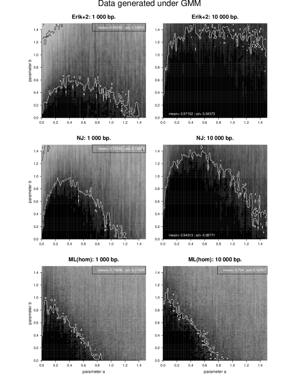
Figure 3: Performance on the tree space of Figure 1.b on data generated under the general Markov model: black is used to represent 100 % of successful topology reconstruction, white to represent 0 %, and different tones of gray the intermediate frequencies. Top: Erik+2; Middle: Neighbor-Joining (paralinear distance); Bottom: ML(hom) estimating the most general homogeneous across lineages continuous-time model. Left: 1 000 bp; Right: 10 000 bp.

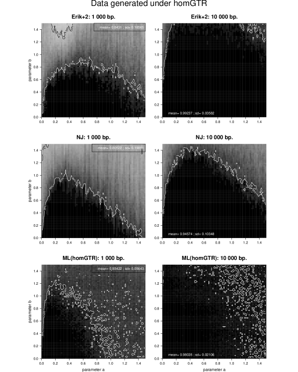
Figure 4: Performance on the tree space of Figure 1.b on data generated under the (homogeneous across lineages) GTR model: black is used to represent 100 % of successful topology reconstruction, white to represent 0 %, and different tones of gray the intermediate frequencies. Top: Erik+2; Middle: Neighbor-Joining (paralinear distance); Bottom: ML(homGTR) estimating homogeneous GTR model. Left: 1 000 bp; Right: 10 000 bp.

Appendix A Supplementary Material

Appendix 1. Bipartition and transition matrices in the Felsenstein zone

Here we illustrate the general situation on alignments corresponding to the Felsenstein zone.

The two matrices on the following page correspond to the bipartition matrices $M_{12|34}(\tilde{p})$ and $M_{13|24}(\tilde{p})$ of an alignment generated under GMM on the tree of Figure 1.a with values $a=0.05$ and $b=1.01$ (Felsenstein zone). In the second matrix, non-zero entries gather around the columns labeled with $AA$, $CC$, $GG$ and $TT$, while in the first matrix, we do not observe such an arrangement. This phenomenon is explained in terms of the short branch length between leaves $2$ and $4$, inducing few mutations between the sequences at these two leaves. This makes the matrix $M_{13|24}(\tilde{p})$ to be closer to rank-4 matrices than $M_{12|34}(\tilde{p})$. Erik+2 corrects this bias by normalizing row and column sums so that all they have the same weight.

The following table displays the Frobenius distance of the bipartition matrices $M_{12|34}$, $M_{13|24}$ and $M_{14|23}$ to the space of matrices with rank $\leq 4$. According to these values, ErikSVD would choose the topology $13|24$ as the right topology, as the corresponding value is the smallest among the values obtained by the 3 topologies. However, applying the correction introduced in Erik+2, the topology $12|34$ is the one to be chosen as correct.

$$\begin{array}[]{c||cccccccccccccccc|c}12|34&AA&AC&AG&AT&CA&CC&CG&CT&GA&GC&GG&GT&TA&TC&TG&TT&+\\ \hline\cr\hline\cr AA&0.128&0.001&0.016&0.006&0.043&0.001&0.005&0.003&0.008&0&0.004&0&0.011&0&0&0.003&0.229\\ AC&0.001&0&0.001&0&0&0.002&0&0&0&0&0&0&0&0&0&0&0.004\\ AG&0.001&0.001&0.021&0.001&0.002&0.002&0.027&0.001&0&0&0.009&0&0.001&0.001&0.001&0.002&0.070\\ AT&0.002&0&0&0.011&0.001&0&0&0.013&0&0&0&0.002&0&0&0&0.039&0.068\\ CA&0.023&0&0.002&0.003&0.005&0&0&0&0&0&0&0.001&0&0&0&0.001&0.035\\ CC&0.001&0.025&0.004&0.002&0.003&0.140&0.011&0.003&0.001&0.026&0.008&0&0&0.012&0.001&0.006&0.243\\ CG&0.001&0.003&0.028&0.002&0&0.0010&0.017&0&0.001&0.002&0.013&0&0.001&0&0.001&0.004&0.074\\ CT&0&0&0.001&0.019&0.001&0.002&0.001&0.029&0&0.001&0&0.006&0&0.003&0&0.055&0.118\\ GA&0.001&0&0&0&0.001&0&0&0&0.001&0&0&0&0&0&0&0&0.003\\ GC&0&0&0&0&0&0&0&0&0&0&0&0&0&0&0&0&0\\ GG&0&0&0.009&0&0&0.001&0.005&0&0&0&0.003&0&0&0&0.001&0.001&0.020\\ GT&0&0&0&0.001&0.001&0&0&0.003&0&0&0&0&0&0&0&0.004&0.009\\ TA&0.010&0&0.001&0&0.001&0&0&0.001&0.001&0&0.001&0&0&0&0.001&0&0.016\\ TC&0&0&0&0.002&0&0.005&0&0&0.001&0&0&0&0&0&0&0.001&0.009\\ TG&0&0.004&0.006&0&0&0.001&0.010&0&0&0&0.003&0.002&0&0&0.001&0.003&0.030\\ TT&0.002&0&0&0.010&0.001&0&0&0.020&0&0&0&0.001&0&0.001&0&0.036&0.071\\ \hline\cr+&0.170&0.034&0.089&0.057&0.059&0.155&0.076&0.073&0.013&0.029&0.041&0.012&0.013&0.017&0.006&0.155&1\end{array}$$

$$\begin{array}[]{c||cccccccccccccccc|c}13|24&\textbf{AA}&AC&AG&AT&CA&\textbf{CC}&CG&CT&GA&GC&\textbf{GG}&GT&TA&TC&TG&\textbf{TT}&+\\ \hline\cr\hline\cr AA&0.128&0.001&0.016&0.006&0.001&0&0.001&0&0.001&0.001&0.021&0.001&0.002&0&0&0.011&0.190\\ AC&0.043&0.001&0.005&0.003&0&0.002&0&0&0.002&0.002&0.027&0.001&0.001&0&0&0.013&0.100\\ AG&0.008&0&0.004&0&0&0&0&0&0&0&0.009&0&0&0&0&0.002&0.023\\ AT&0.011&0&0&0.003&0&0&0&0&0.001&0.001&0.001&0.002&0&0&0&0.039&0.058\\ CA&0.023&0&0.002&0.003&0.001&0.025&0.004&0.002&0.001&0.003&0.028&0.002&0&0&0.001&0.019&0.114\\ CC&0.005&0&0&0&0.003&0.140&0.011&0.003&0&0.001&0.017&0&0.001&0.0020&0.001&0.029&0.213\\ CG&0&0&0&0.001&0.001&0.026&0.008&0&0.001&0.002&0.013&0&0&0.001&0&0.006&0.059\\ CT&0&0&0&0.001&0&0.012&0.001&0.006&0.001&0&0.001&0.004&0&0.003&0&0.055&0.084\\ GA&0.001&0&0&0&0&0&0&0&0&0&0.009&0&0&0&0&0.001&0.011\\ GC&0.001&0&0&0&0&0&0&0&0&0.001&0.005&0&0.001&0&0&0.003&0.011\\ GG&0.001&0&0&0&0&0&0&0&0&0&0.003&0&0&0&0&0&0.004\\ GT&0&0&0&0&0&0&0&0&0&0&0.001&0.001&0&0&0&0.004&0.006\\ TA&0.010&0&0.001&0&0&0&0&0.002&0&0.004&0.006&0&0.002&0&0&0.010&0.035\\ TC&0.001&0&0&0.001&0&0.005&0&0&0&0.001&0.010&0&0.001&0&0&0.020&0.039\\ TG&0.001&0&0.001&0&0.001&0&0&0&0&0&0.003&0.0020&0&0&0&0.001&0.009\\ TT&0&0&0.001&0&0&0&0&0.001&0&0&0.001&0.003&0&0.001&0&0.036&0.043\\ \hline\cr+&\textbf{0.233}&0.002&0.030&0.018&0.007&\textbf{0.210}&0.025&0.014&0.007&0.016&\textbf{0.155}&0.016&0.008&0.007&0.002&\textbf{0.249}&1\end{array}$$

Appendix 2. Supplementary material

Performance of ErikSVD

Figure S1. Performance of ErikSVD on the tree space of Figure 1.b on data generated under GMM: black is used to represent 100 % of success, white to represents 0 % and different tones of gray the intermediate frequencies. Parameters $a$ and $b$ refer to the branch lengths of the tree of Figure 1.a, where $c$ is set equal to $a$.

Performance on GTR data (500 bp.)

Figure S2. Performance of ErikSVD, Erik+2, ML and NJ on the tree space of Figure 1.b on alignments of 500 bp. generated under homGTR; black is used to represent 100 % of success, white to represents 0 % and different tones of gray the intermediate frequencies. Top Left: ErikSVD; Top Right: Erik+2; Bottom Left: ML estimating homogenous GTR model –ML(homGTR); Bottom Right: Neighbor-Joining (paralinear distance).

Performance of Erik+2 with $m=2$ on unmixed data

Figure S3. Performance of Erik+2 with $m=2$ on the tree space of Figure 1.b on data generated under GMM with homogeneity across sites for length 1 000; black is used to represent 100 % of success, white to represents 0 % and different tones of gray the intermediate frequencies. Parameters $a$ and $b$ refer to the branch lengths of the tree of Figure 1.a, where $c$ is set equal to $a$.

Performance of Erik+2 with $m=1,2$

Figure S4. Percentage of correctly inferred trees by Erik+2 with $m=1$ and $m=2$ on alignments of lengths 1 000, 10 000 and 100 000 bp. shown from top to bottom. a) Performance of Erik+2 with $m=1$ and $m=2$ on data generated under GMM on the tree of Figure 1.a with $a=0.05$, $b=0.75$, and varying the internal branch length $c$. b) Performance of Erik+2 (with $m=1$) and Erik+2 (with $m=2$) on data generated under GTR model with continuous Gamma-rates and parameter $\alpha$ varying between 0.1 and 2 on the 4-taxa tree of Figure 1.a with branch lengths $a=c=0.05$ and $b=0.75$.

References

- Allman and Rhodes (2007) E. S. Allman and J. A. Rhodes. Phylogenetic invariants. In O. Gascuel and M. A. Steel, editors, Reconstructing Evolution. Oxford University Press, 2007.
- Allman and Rhodes (2008) E. S. Allman and J. A. Rhodes. Phylogenetic ideals and varieties for the general Markov model. Adv. in Appl. Math., 40(2):127–148, 2008. ISSN 0196-8858.
- Barry and Hartigan (1987) D. Barry and J. A. Hartigan. Statistical analysis of hominoid molecular evolution. Statistcal Sciences, 2(2):191–207, 1987.
- Casanellas and Fernández-Sánchez (2007) M. Casanellas and J. Fernández-Sánchez. Performance of a new invariants method on homogeneous and nonhomogeneous quartet trees. Mol. Biol. Evol., 24:288–293, 2007.
- Casanellas and Fernández-Sánchez (2010) M. Casanellas and J. Fernández-Sánchez. Relevant phylogenetic invariants of evolutionary models. J. Math. Pure. Appl., 96:207–229, 2010.
- Casanellas et al. (2012) M. Casanellas, J. Fernández-Sánchez, and A. Kedzierska. The space of phylogenetic mixtures for equivariant models. Algorithms for Molecular Biology, 7:33, 2012.
- Cavender and Felsenstein (1987) J. A. Cavender and J. Felsenstein. Invariants of phylogenies in a simple case with discrete states. J. Class., 4:57–71, 1987.
- Demmel (1997) J. W. Demmel. Applied numerical linear algebra. Society for Industrial and Applied Mathematics (SIAM), Philadelphia, PA, 1997. ISBN 0-89871-389-7. doi: 10.1137/1.9781611971446. URL http://dx.doi.org/10.1137/1.9781611971446.
- Dutheil and Boussau (2008) J. Dutheil and B. Boussau. Non-homogeneous models of sequence evolution in the Bio++ suite of libraries and programs. BMC Evolutionary Biology, 8(1):255, 2008.
- Eckart and Young (1936) C. Eckart and G. Young. The approximation of one matrix by another of lower rank. Psychometrika, 1(3):211–218, 1936.
- Eriksson (2005) N. Eriksson. Tree construction using singular value decomposition. In Algebraic statistics for computational biology, pages 347–358. Cambridge Univ. Press, New York, 2005.
- Felsenstein (1978) J. Felsenstein. Cases in which parsimony or compatibility methods will be positively misleading. Systematic Z, 27:401–410, 1978.
- Felsenstein (2004) J. Felsenstein. Inferring Phylogenies. Sinauer Associates, 2004.
- Fitch (1986) W. M. Fitch. An estimation of the number of invariable sites is necessary for the accurate estimation of the number of nucleotide substitutions since a common ancestor. Progress in clinical and biological research, 218:149–159, 1986.
- Foster (2004) P. G. Foster. Modeling compositional heterogeneity. Syst. Biol., 53(3):485–495, 2004.
- Galtier and Gouy (1998) N. Galtier and M. Gouy. Inferring pattern and process: maximum-likelihood implementation of a nonhomogeneous model of dna sequence evolution for phylogenetic analysis. Mol. Biol. Evol., 15:871–879, 1998.
- Ho and Jermiin (2004) S. Y. Ho and L. S. Jermiin. Tracing the decay of the historical signal in biological sequence data. Systematic Biology, 53(4):623–637, 2004.
- Holland et al. (2013) B. R. Holland, P. D. Jarvis, and J. G. Sumner. Low-parameter phylogenetic inference under the general Markov model. Systematic Biology, 63(1):78–92, 2013.
- Huelsenbeck (1995) J. P. Huelsenbeck. Performance of phylogenetic methods in simulation. Syst. Biol., 44:17–48, 1995.
- Jayaswal et al. (2005) V. Jayaswal, L. S. Jermiin, and J. Robinson. Estimation of phylogeny using a general Markov model. Evolutionary Bioinformatics Online, 1:62–80, 2005.
- Jayaswal et al. (2011) V. Jayaswal, L. S. Jermiin, L. Poladian, and J. Robinson. Two stationary nonhomogeneous Markov models of nucleotide sequence evolution. Systematic Biology, 60(1):74–86, 2011.
- Jayaswal et al. (2014) V. Jayaswal, T. K. Wong, J. Robinson, L. Poladian, and L. S. Jermiin. Mixture models of nucleotide sequence evolution that account for heterogeneity in the substitution process across sites and across lineages. Systematic Biology, 63(5):726–742, 2014. doi: 10.1093/sysbio/syu036.
- Kedzierska and Casanellas (2012) A. M. Kedzierska and M. Casanellas. Gennon-h: Generating multiple sequence alignments on nonhomogeneous phylogenetic trees. BMC Bioinformatics, 13(1):216, 2012.
- Kolaczkowski and Thornton (2004) B. Kolaczkowski and J. Thornton. Performance of maximum parsimony and likelihood phylogenetics when evolution is heterogeneous. Nature, 431:980?984, 2004.
- Kück et al. (2012) P. Kück, C. Mayer, J.-W. Wagele, and B. Misof. Long branch effects distort maximum likelihood phylogenies in simulations despite selection of the correct model. PLoS One, 7(10), 2012. DOI 10.1371/journal.pone.0036593.
- Lake (1987) J. A. Lake. A rate-independent technique for analysis of nucleic acid sequences: evolutionary parsimony. Mol. Biol. Evol., 4:167–191, 1987.
- Lake (1994) J. A. Lake. Reconstructing evolutionary trees from DNA and protein sequences: Paralinear distances. Proceedings of the National Academy of Sciences, 91:1455–1459, 1994.
- Phillips et al. (2004) M. J. Phillips, F. Delsuc, and D. Penny. Genome-scale phylogeny and the detection of systematic biases. Molecular Biology and Evolution, 21(7):1455–1458, 2004. doi: 10.1093/molbev/msh137.
- Rambaut and Grassly (1997) A. Rambaut and N. Grassly. Seq-Gen: An application for the Monte Carlo simulation of DNA sequence evolution along phylogenetic trees. Comput. Appl. Biosci., 13:235–238, 1997.
- Ranwez and Gascuel (2001) V. Ranwez and O. Gascuel. Quartet-based phylogenetic inference: Improvements and limits. Molecular Biology and Evolution, 18(6):1103–1116, 2001.
- Rhodes and Sullivant (2012) J. A. Rhodes and S. Sullivant. Identifiability of large phylogenetic mixture models. Bulletin of Mathematical Biology, 74(1):212–231, 2012. ISSN 0092-8240.
- Rokas et al. (2003) A. Rokas, B. L. Williams, N. King, and S. B. Carroll. Genome-scale approaches to resolving incongruence in molecular phylogenies. Nature, 425, 2003.
- St. John et al. (2003) K. St. John, T. Warnow, B. M. E. Moret, and L. Vawter. Performance study of phylogenetic methods: (unweighted) quartet methods and neighbor-joining. J. Algorithms, 48(1):173–193, 2003.
- Stefankovic and Vigoda (2007) D. Stefankovic and E. Vigoda. Pitfalls of heterogeneous processes for phylogenetic reconstruction. Systematic biology, 56(1):113–24, Feb. 2007.
- Swofford et al. (2001) D. L. Swofford, P. J. Waddell, J. P. Huelsenbeck, P. G. Foster, P. O. Lewis, and J. S. Rogers. Bias in phylogenetic estimation and its relevance to the choice between parsimony and likelihood methods. Systematic Biology, 50(4):525–539, 2001.
- Tateno et al. (1994) Y. Tateno, N. Takezaki, and M. Nei. Relative efficiencies of the maximum-likelihood, neighbor-joining, and maximum-parsimony methods when substitution rate varies with site. Molecular biology and evolution, 11(2):261–77, 1994.
- Yang (1993) Z. Yang. Maximum-likelihood estimation of phylogeny from dna sequences when substitution rates differ over sites. Molecular Biology and Evolution, 10(6):1396–1401, 1993.
- Yang (1994) Z. Yang. Maximum likelihood phylogenetic estimation from DNA sequences with variable rates over sites: approximate methods. J. Mol. Evol., 39:306–314, 1994.
- Yang (1997) Z. Yang. PAML: a program package for phylogenetic analysis by maximum likelihood. Bioinformatics, 13:555–556, 1997.
- Yang and Roberts (1995) Z. Yang and D. Roberts. On the use of nucleic acid sequences to infer early branchings in the tree of life. Mol. Biol. Evol., 12:451–458, 1995.