Gaussian Random Functional Dynamic Spatio-Temporal Modeling of Discrete-Time Spatial Time Series Data
Abstract
Discrete-time spatial time series data arise routinely in meteorological and environmental studies. Inference and
prediction associated with them are mostly carried out using any of the several variants of the linear state space
model that are collectively called linear dynamic spatio-temporal models (LDSTMs). However, real world environmental
processes are highly complex and are seldom representable by models with such simple linear structure. Hence,
nonlinear dynamic spatio-temporal models (NLDSTMs) based on the idea of nonlinear observational and evolutionary
equations have been proposed as an alternative. However, in that case, the caveat lies in selecting the specific
form of nonlinearity from a large class of potentially appropriate nonlinear functions. Moreover, modeling by
NLDSTMs requires precise knowledge about the dynamics underlying the data. In this article, we address
this problem by introducing the Gaussian random functional dynamic spatio-temporal model (GRFDSTM).
Unlike the LDSTMs or NLDSTMs, in GRFDSTM both the functions governing the observational and evolutionary equations
are composed of Gaussian random functions. We exhibit many interesting theoretical properties of the GRFDSTM and
demonstrate how model fitting and prediction can be carried out coherently in a Bayesian framework.
We also conduct an extensive simulation study and apply our model to a real, pollution data over Europe.
The results are highly encouraging.
Keywords: Evolutionary equation; Gaussian process; Gibbs sampler; MCMC; Observational equation; Posterior predictive distribution; State-space model.
AMS 2000 Subject Classification: Primary 62M20, 62M30; Secondary 60G15.
1 Introduction
Spatio-temporal modeling has received much attention in recent years. Particularly, the rise in global temperature being a major environmental concern, scientists are now taking keen interest in developing appropriate statistical models to study such climatic phenomena [23, 35, 47, 48, 51, 56]. Other closely related meteorological phenomena, that are also drawing much attention of modelers, are rainfall [12, 49] and precipitation (mist, snowfall, sulphate, nitrate [46] etc.) across different regions. Apart from meteorology, challenging spatio-temporal data also arise from environmental and ecological science. To mention a few, studies on ground level concentration of ozone [10, 20, 29, 33], [28, 30], [2] and PM [41] related air pollution, species distribution over a region [11], change in land usage pattern over time [17], etc.
While the term spatio-temporal data encompasses the above few and includes many other different types of data, the above-mentioned ones belong to a particularly interesting class called discrete-time spatial time series data. Typically, they are obtained by collecting observations at arbitrary but fixed spatial locations at times . The data can be represented as , and then we have a whole set of time series, one for each spatial location. Although in reality, the data is available only at finitely many spatial locations (generally called monitoring sites), it is conceptually always useful to assume the existence of time series at every spatial location. An alternative view is to consider it as a time varying spatial random field. The problem facing the statistician is to develop an appropriate model, infer about the spatio-temporal process and possibly predict at new sites based on this partial realization.
In what follows, we review some existing models and discuss the advantages and problems associated with them. Then we develop the Gaussian random functional dynamic spatio-temporal model (GRFDSTM) and study its theoretical properties in much detail. We demonstrate how model fitting and prediction can be done coherently using a Bayesian approach. Finally, we examine its performance in an extensive simulation study and apply it to an pollution dataset over Europe, and obtain very encouraging results. The proofs of all our mathematical results are deferred to the Appendix.
2 Existing Approaches for Discrete-Time Spatial Time Series Data
As already mentioned, discrete-time spatial time series data consists of observations taken at some arbitrary but fixed spatial locations at times . Note that any method applicable to them can easily be extended to data collected at non equispaced time points. Hence, for the sake of simplicity we confine ourselves only to equispaced time points.
There exist two different perspectives from which one can develop a model for such data. One is the marginal approach, in which one develops a joint distribution for . In the case of the Gaussian model, this amounts to specifying a spatio-temporal mean function and covariance function. The other approach relies on specifying the conditional distribution of the current process realizations given the past process realizations. Although theoretically it is equivalent to specifying the conditional distribution or the marginal distribution, one being derivable from the other, the conditional approach being more closer to the etiology of the phenomena under study, is preferred over the marginal one. For more discussions on this issue interested reader may look into the book by [13]. In fact, [13] covers very wide range of materials on dynamic spatio-temporal modeling and also serves as the main resource for many of the models that we consider here.
Although there exists a vast literature on marginal models, here we mention only a few of them. [45] proposed a regional-effects model for the analysis of stratospheric ozone data. Later, [9] considered the spatio-temporal random effect and extended it to the following model (see equation 6.16 on the page 306 of [13])
where is the random time effect common to all spatial locations, is the random regional time effect common to all locations belonging to the th region, is the spatio-temporal random effect and is a spatio-temporal white noise process representing the microscale spatio-temporal variability. Another interesting marginal model that hinges not only on the spatio-temporal effect but also incorporates useful covariate information is the following spatio-temporal hedonic model for house prices proposed by [24]:
Here, is the log selling price, is the common time effect for all the locations, is the spatial effect, is the Gaussian white noise and is the design matrix containing useful covariate information. This form allows spatio-temporally varying coefficients, which is perhaps more than what is required. Hence, is frequently adopted. Setting yields an extension of the model proposed by [37].
Akin to the marginal approach several models for the conditional distribution have been proposed and most of them are based on the idea of linear state space models in time series. These models are generally referred to as linear dynamic spatio-temporal models (LDSTMs). A common representative form for them would be
where controls the temporal effect and handles the spatial variation. The design matrix either consists of deterministic functions of locations or important covariate information associated with the locations. The observed data arise from the process , which is temporally driven by the latent (or, state) process and the temporal evolution of is given by some suitable conditional model, preferably a Markovian one. [53] applied the above model in the environmental context, where they chose to define as a linear combination of basis functions of the location . Their model is attractive in being applicable to any dataset that is continuous in space and discrete in time. [58] used the same model in their dimension reduction approach. However, they obtained the model from a more general underlying process. [50] also used this model, but without the error term. The scope of the model is widened further as [38] allowed the columns of to vary as random functions of locations. Although developed primarily for modeling Gaussian spatial time series data, LDSTMs are easily amenable to non-Gaussian data. Particularly, it can be modified as follows, so as to be suitable for spatio-temporal data that are associated with an exponential family model
Here is a known, twice differentiable function, is a known function and is a scalar dispersion parameter.
All these models are dynamically specified but the dynamics remain invariant across the space. Significant extension can be achieved by allowing the state variable to vary across space. This obviously implies a substantial increase in the number of parameters and may lead to identifiability problem. Putting restrictions on the parameter space keeps the problem manageable. [42] proposed such a spatially varying coefficient dynamic model where they took . The common trend evolves dynamically with time but the spatio-temporal part are iid Gaussian processes on space. [5] considered a more general model in the environmental context where both and vary dynamically with respect to time. They used this model in the context of regression. [33] used a similar model additionally equipped with seasonal components to analyze a spatio-temporal ozone dataset. The spatially varying state variables for all these LDSTMs can be represented as
However, a number of authors proposed an apparently different form for the evolution of . They assumed that
where is a redistribution kernel that determines how the state variables at the previous time point influence the state variables at present. Typically, spatially nearer observations get more weight. Although, it appears to be very different from the form considered earlier, a discrete convolution based approximation to the integral would yield that usual form. [58] considered the above formulation in their dimension reduction approach and [52] considered it in the context of temperature data modeling.
Model fitting for LDSTMs can be carried out either by the hierarchical Bayesian approach or by classical Kalman filtering. [58, 32, 39] used classical Kalman filter or its variations whereas [53, 49, 54, 33, 5] considered the hierarchical Bayesian approach. For more on LDSTMs an excellent reference would be [25].
So far we have considered dynamic spatio-temporal models whose temporal evolution can be described by linear equations. However, real life environmental processes are complex and require much more sophistication in model specification. In particular, processes like precipitation, deposition, etc. are driven by complex interactions among atmospheric processes and are best represented by nonlinear models. An LDSTM model as considered above would be simply unsuitable in this situation. Apart from atmospheric processes, sometimes sea-surface temperature data is modeled by nonlinear dynamic spatio-temporal models (NLDSTMs) owing to the complex dynamics of sea waves, that influence it heavily. Also, many processes in the context of growth curve modeling exhibit state-dependent or density-dependent growth, e.g., for some nonlinear growth function (e.g., logistic, Ricker, Beverton-Holt, etc.). In addition, many processes exhibit what is sometimes referred to as nonlinear advection, e.g., in one spatial dimension, (see [13]). More general nonlinear dynamic spatio-temporal models are required to accommodate such processes, among others. [49] considered such a truncation based NLDSTM for modeling a Venezuelan rainfall dataset, given as follows:
where is the state process and is a time varying parameter associated with the truncation equation. A more general formulation for this model can be written as (see equation 7.39 on page 380 of [13])
where is a spatial-temporal noise process. The above model assumes that the observational equation that connects the observed process with the state or latent process , is nonlinear. Instead of that, nonlinearity can be introduced into the evolutionary equation. In that case, we would have
where is some appropriate nonlinear function. [13] discussed nonlinear state-dependent models which are time varying versions of it. Often the nonlinear function is taken to be a threshold function as follows:
where is a function of a time varying parameter , and , is the condition under which the th equation is to be followed (see equation 7.69 on page 406 of [13]). An example of such a model is given by [8] with regard to long-lead forecasting of tropical Pacific sea surface temperature. [34] used such a model in atmospheric application and [31] employed them for the analysis of an ecological dataset. Another interesting class of NLDSTM, that [60] (also see [13]) referred to as the General Quadratic Nonlinear (GQN) Model, is given by
where is a linear combination of the process at the previous time and
contains quadratic interactions of the process and potentially some transformation of the lagged process, at the previous time.
The model is flexible enough to accommodate nonlinear transformations of the process through the function ,
which might depend upon the unknown parameter vector . GQN constitutes a very rich class
of models and many complex process models including the one considered by [7]
for the so-called quasi-geostrophic flow in the ocean, are special cases of it. [59] considered an
extension of GQN by incorporating higher order polynomial interaction terms in the following way:
It is called the General Polynomial Nonlinear (GPN) model. For an excellent overview about such NLDSTMs the reader may look into chapter 7 of [13].
NLDSTMs provide us with a way out when the usual LDSTMs turn out to be too naive for the phenomena under study, but that too comes with a cost. The issues of dimensionality and efficient parametrization present the most significant challenges for statistical modeling of LDSTMs and these issues get even more critical for NLDSTM’s. However, what is more daunting is that without very precise knowledge of the underlying dynamics, it is almost impossible to elicit an appropriate nonlinear model from a large class of probable nonlinear functions. A selected nonlinear model, that is unsuitable for the physical process under study, would show grossly poor predictive performance. Seemingly irrelevant departure from reality at the level of model specification cumulates over time and the outcome may be devastating.
3 Gaussian Random Functional Dynamic Spatio-Temporal Model
As already discussed, a focal issue for the NLDSTMs is the selection of the form of nonlinearity, and such a task is highly non-trivial. We propose a dynamic spatio-temporal model where both the observational and evolutionary equations are random functions. Hence, we no longer have to decide about the specific functional forms; instead, all we need to do is to ensure that the probabilistic law for the random function is so chosen that it gives enough probability to a set of functions that seem potentially appropriate for the data at hand. Moreover, unlike the LDSTMs or NLDSTMs where the functional form is fixed, a random functional form is more adaptable to the data and expected to represent the true underlying process, which may be complex and highly nonlinear, more accurately. As the probabilistic law for those random functions, we specify appropriate Gaussian processes. The motivation for choosing Gaussian process comes from the fact that Gaussian processes are good natural priors for nonparametric regression and classification problems and under increasingly dense observations, the true shape of the arbitrary function or the classifier can be captured accurately, a posteriori [44]. Later we shall see how the proposed Gaussian random functional dynamic spatio-temporal model (we refer to our model as GRFDSTM) is connected to a Bayesian nonparametric function estimation problem. Besides, already there is a very rich mathematical theory for Gaussian process [1] which can be utilized to explore properties of GRFDSTM. Many elegant mathematical results, which hold true for Gaussian random functions, may be lost if we consider some other random functions, i.e., Levy random functions, Elliptic random functions etc.
We assume that the observed spatio-temporal process (equivalently, ) is driven by an unobserved spatio-temporal state process which itself is evolving in time. Our model can be described in the following way:
| (1) | ||||
| (2) | ||||
| (3) |
where and . In the above, “GP” stands for “Gaussian process” and “GRF” stands for “Gaussian random function”. Here is a spatial Gaussian process on ; and are temporally independent and identically distributed spatial Gaussian processes on , and and are Gaussian random functions on . They are all independent of each other. Note that, in the LDSTMs and NLDSTMs discussed in the previous section, the state process is denoted by or and commonly refer to the covariate information, whereas for GRFDSTM we choose to denote the state process by , which resembles the notation used for state space models in classical time series literature.
The specification (2) is very crucial since it determines the nonlinear dynamics of the model. In nature we encounter such nonlinear function in population ecology where measures vegetation density at location at time . Then is linked to the population size of a herbivorous species that feed on it, through some complex nonlinear function . The population size of the herbivorous species on the other hand, dynamically changes according to a discretized spatial Lotka-Voltera type model.
where denotes the population size of a carnivorous species that hunt the herbivorous species. So, in this case through a very complex nonlinear function which is not even writable in closed form. Another instance of such nonlinear evolutionary transformation can be found in oceanography where the sea surface temperature depends on the ocean stream function . The ocean stream function varies dynamically through some complex nonlinear equation referred to as quasi-geostrophic (QG) equation (see [7])
Again, discretized version of this equation leads to a very complex nonlinear evolutionary transformation .
The GRFDSTM can be connected to a Bayesian nonparametric function estimation problem in the following way. Suppose, we want to study a spatio-temporal process . However, all that we have is data , which is a masked version of . Such masked data are routinely encountered in the study of signals, images, videos, etc. Suppose that is dynamically changing with time and the dynamics can be modeled by some complex, possibly nonlinear function . Then continuity is the minimal requirement for such a function . We further assume that the masking is also described by some continuous transformation . Now, the problem facing the statistician is to estimate the two unknown functions (or alternatively infinite dimensional parameters) and recover the true signal . To solve the problem in the Bayesian way we must elicit priors on the infinite dimensional function space of all real-valued continuous functions on the real line, i.e., . Suppose, we specify a Gaussian process prior on the parameter space . Then, if we consider the conditional distribution of , where is the hyper-parameter associated with the Gaussian process priors, it is the same as the GRFDSTM. Although the purpose of this hierarchical Bayesian model for function estimation is to identify and and recover the original signal , which is quite different than the purpose the GRFDSTM serves, i.e., prediction possibly at a new spatio-temporal location , the following duality between the two models
| [good estimators of and | [good predictors of at the spatio- | ||
| for the hierarchical Bayesian model] | temporal location for the GRFDSTM] |
gives us the intuition that a GRFDSTM might work well.
Finally, to completely specify the GRFDSTM, we need to describe the parameters associated with the Gaussian random functions and the spatial Gaussian processes. We assume that the Gaussian random function has the mean function of the form (where are suitable parameters) and has isotropic covariance kernel of the form , where is a positive definite function. It again consists of parameters that determine the smoothness of the sample paths of . Moreover, is such that the centered Gaussian random function with covariance kernel has continuous sample paths. This assumption of sample path continuity is required due to some technical reasons and is very minimal in the sense that all popular isotropic covariance kernels satisfy it. Typical examples of are exponential, powered exponential, Gaussian, Matérn etc. (see, for example, Table 2.1 of [3] for other examples of such covariance kernels). Similarly, parameters and are associated with the Gaussian random function .
The zero mean spatial Gaussian processes and have covariance kernels and respectively, which are also of similar form.
Regarding the spatial Gaussian process associated with , we assume a continuous mean process of the form and isotropic covariance kernel . For convenience, we introduce separate notations for the mean vector and the covariance matrix associated with , where are the spatial locations where the data is observed. We denote them by and respectively.
From (1) and (2) it is not difficult to see that our model boils down to a simple LDSTM with no covariate if the process variance associated with the Gaussian random functions (denoted by and ) become 0. The model equations (1) and (2) then reduce to the following form
| (4) | ||||
| (5) | ||||
| (6) |
where and . Although we develop the GRFDSTM for equispaced time points, simple modification of this model can handle non equispaced time points as well. However, for the sake of simplicity and brevity, in this article, we shall consider only equispaced time points. Lastly, it is also possible to consider nonlinear mean function for and . This formulation would work well, provided one already has strong prior knowledge about the form of the nonlinear dynamics behind the process. However, under little or no knowledge about the process, we strongly suggest sticking to the linear mean functions.
The GRFDSTM is in spirit very similar to spatio-temporal generalized additive models (STGAM) [28, 30]. A typical STGAM looks like the following
Like the GRFDSTM, the STGAM also model the data without assuming linear or specific nonlinear form for and , thereby modeling the spatial and temporal trend nonparametrically. However, the main difference between the GRFDSTM and the STGAM is that the former is a conditional approach and assumes flexible nonparametric form for the dynamic (conditional) structure of the space-time model whereas the latter is a marginal approach and stresses flexible modeling of the trend in space and time and the interaction (marginal and joint) terms.
3.1 Some Measurability and Existential Issues
Before we proceed to explore the properties of GRFDSTM, we need to ensure that a family of valid (measurable) spatio-temporal stochastic processes is induced by the proposed model. Only then it can be used as a statistical model for real world physical processes. In general, such measurability issues are almost always trivially satisfied by statistical models and so, never discussed in detail. But in this case, we need to show that are jointly measurable for any and any set of spatial locations , and this is not a trivial problem. The difficulty is that when and both are random, need not be a measurable or valid random variable. It is the sample path continuity of , which compels to be measurable.
Proposition 3.1.
The GRFDSTM defines a family of valid (measurable) spatio-temporal processes on .
Once it is ensured that the proposed model induces a family of valid spatio-temporal processes, we look into some other important aspects like the joint distributions of state variables and observed variables, covariance structure of the observed process etc. Note that although we develop the GRFDSTM assuming that the spatial dimension is , the construction and all the subsequent results go through for as well.
3.2 Joint Distribution of the Variables
Due to the implicit hierarchical structure of the GRFDSTM, the joint distribution of the observed variables is non-Gaussian. But even before considering that, we want to find out the joint distribution of the state variables. A closed form joint pdf for the state variables is necessary for MCMC based posterior inference.
Theorem 3.2.
Suppose that the spatio-temporal process is observed at locations for times . Then the joint distribution of the state variables is non-Gaussian and has the pdf
where and are already defined to be the mean vector and the covariance matrix of , and
where the elements of are obtained from the purely spatial covariance function and the elements of are obtained from the covariance function in the following way :
the th entry of is and the th entry of is where and .
Although the appearance of the probability density function resembles that of a multivariate Gaussian density, the involvement of in renders it non-Gaussian. In the extreme case when the process variance () of the Gaussian random function is 0, becomes a block diagonal matrix with identical blocks and the joint density becomes Gaussian. In the formation of , the part corresponds to linear evolution and Gaussianity whereas the component corresponds to departure from linearity. In fact, it is also responsible for making the pdf a non-Gaussian one.
Moreover, it is also clear from the form of the density function that the temporal aspect is imposed on the model through both the location function and the scale function associated with the latent process, making the GRFDSTM a very flexible spatio-temporal model.
The interesting property that the observed spatio-temporal process is also non-Gaussian, is a consequence of both of the facts that the state variables are non-Gaussian and the GRFDSTM has an implicit hierarchical structure. We have the following theorem in this regard:
Theorem 3.3.
Suppose that the spatio-temporal process is observed at locations for times .
Then the following hold true:
(a) The joint distribution of the observed variables is a Gaussian mixture and has the following density
where the mixing density is obtained by marginalizing the pdf derived at Theorem 3.2 with respect to
the variables and the
th entry of is given by where and .
(b) In the extreme case, when the process variance () and ()
of each of the Gaussian random function and are 0,
the joint distribution turns into Gaussian.
The implicit hierarchical structure implies that the observed spatio-temporal process is a mixture of Gaussian processes which subsequently implies that GRFDSTM can flexibly accommodate both Gaussian and non-Gaussian distributions for spatio-temporal data. In fact several authors have already used the mixture distribution approach to produce non-Gaussian models for spatial and spatio-temporal data [22, 43].
3.3 Dependence and Covariance Structure
As is evident from Theorem 3.3, the observed process is non-Gaussian for all but a few special cases. Hence, the covariance function no longer characterizes the dependence structure completely. However, the covariance function, which characterizes the linear dependence structure, still might give us valuable insight about the process, particularly in the case of small departure from linearity ( and are small) and so it is worthwhile to take a deeper look into that. However, even before delving into a deeper study of the covariance function and some related issues like nonstationarity and nonseparability, a more basic question is whether the process is light-tailed, that is, whether or not all the coordinate variables have finite variance. From Theorem 3.3 we see that the observed variables are distributed as a Gaussian mixture and Gaussian mixtures sometimes can give rise to heavy-tailed distributions. So, an answer to the above question is not immediately available. In what follows, we show that the process is light-tailed and the covariance function is nonstationary and nonseparable.
Theorem 3.4.
(a) The observed spatio-temporal process is light-tailed in the sense that all the coordinate variables have finite variance.
(b) The covariance function of the observed spatio-temporal process is
nonstationary and nonseparable for any .
Although the GRFDSTM yields a nonstationary and nonseparable covariance function, an obvious limitation is that no closed form expression for the covariance function is available. This problem, however, exists in many other spatio-temporal models including the convolution models, deformation models, complex DSTM models, etc., where a closed form covariance function is available only in very few special cases. In fact, the direct construction of spatio-temporal covariance function is the only approach that is always guaranteed to yield a closed form covariance function.
Besides, from the prediction point of view, this is not a serious problem since all that we need are the posterior predictive distributions at unmonitored locations at arbitrary points of time, which do not require closed form expression of the covariance function.
However, we still strive to find some closed form expression and are partially successful in the sense that when our model is approximately linear (in some suitable sense to be described later), the covariance function is approximately a geometric function of time lag.
3.3.1 Approximate Form of the Covariance Function
Here, in Theorem 3.5, we show that if the process variances () and () are small, then under a minor assumption, the covariance function is approximately a geometric function of time lag. This result is mainly of theoretical interest.
Theorem 3.5.
Assume that . Then for given arbitrarily small, such that for the covariance between and , denoted by , is of following form:
The assumption restricts the latent process within the class of nonexplosive spatial AR models. Although this class is fairly large, it misses some interesting spatio-temporal processes like the spatial random walk. Spatial random walk, which is temporally nonstationary, is used extensively in econometric applications.
Note that no such closed form expression is available if we consider the behaviour of with respect to increasing spatial lag, i.e., . Empirical simulations, however, suggest that decays to as and the rate of decay depends on the specific form of the covariance kernels used in the GRFDSTM. Specifically, if we use the squared exponential covariance kernels for all the associated Gaussian random functions and processes, then exhibits short range dependence and decays very fast to as .
3.4 Sample Path Properties
So far, we have discussed the finite dimensional properties of the spatio-temporal process . But finite dimensional properties alone are not sufficient to characterize any arbitrary general stochastic process. Two stochastic processes with completely different sample path behavior may have identical finite dimensional distributions and properties. We demonstrate this through the following simple example (see also [1]):
Let us consider two spatio-temporal processes and defined on the same probability space in the following way: for all , and for all and otherwise. Then one can show that for any fixed , has continuous sample path with probability whereas has discontinuous sample path with probability . However, both and have exactly the same finite-dimensional distributions.
In the light of the above, we decide to explore the path properties of . The first part of the following theorem states that has continuous sample paths and the second part says that moreover, under additional smoothness assumptions regarding the covariance functions, it will have smooth sample paths.
Theorem 3.6.
(a) The spatio-temporal process has continuous sample paths.
(b) Assume that the covariance functions satisfy the
additional smoothness assumption that the centered Gaussian processes with these covariance
functions have times differentiable sample paths. Then the non-Gaussian
spatio-temporal process also have times differentiable sample paths.
So, the spatial surface generated by the GRFDSTM at any time point is continuous and unless the spatial surface interpolating the data points is extremely jagged indicating multiple points of discontinuity, any spatio-temporal data can be modeled reasonably adequately by the GRFDSTM. A stronger statement, however, is made in the second part of the theorem. It says that if the covariance functions are sufficiently smooth then the sample paths of the process are also smooth and their degrees of smoothness depend on the degree of smoothness of the covariance functions. Immediate to the above theorem we have the following corollary associated with two very popular classes of covariance functions.
Corollary 3.7.
(a) If all the covariance kernels associated with GRFDSTM, belong to the Matérn family whose smoothness parameter
is , then will have many time differentiable sample paths.
Here, for any , denotes the smallest integer greater than or equal to .
(b) If all the covariance kernels associated with GRFDSTM, are chosen to be squared exponential,
then will have infinitely many times differentiable sample paths.
It is a well known fact that the sample paths of a centered Gaussian process, whose covariance function is Matérn with smoothness parameter , are times differentiable (see page 23 of [25]).
Hence, part (a) of Corollary 3.7 follows. Part (b) follows from the facts that squared exponential covariance function is essentially Matérn with smoothness parameter and sample paths of a centered Gaussian process with squared exponential covariance function are infinitely many times differentiable. Hence, when we have strong evidence from the data or prior knowledge that the data generating spatial surface is neither too rough nor too smooth, and also have some idea regarding the degree of smoothness of the spatio-temporal process, then we may choose all the covariance functions from the Matérn family with some appropriate specific value of .
4 Identifiability Issues and Sharpening the Model Description
The GRFDSTM is more like an umbrella term used for a general modeling strategy, rather than a single model. Hence, a deeper investigation of the identifiability issue requires more specific model description. First recall that, associated with the mean function of the GRFs and , we have four parameters . The vector parameter is associated with the initial state process. The dependence structure is specified through some isotropic covariance kernels. Note that, till now we have not specified any particular form for the isotropic covariance kernel. However, to address identifiability we need to fix the covariance functions. Although any reasonable isotropic covariance kernel that satisfies the mild regularity conditions mentioned in Section 3 can be used in the GRFDSTM, for the sake of simplicity we consider the squared exponential covariance kernel with the representation . Associated with five covariance kernels we have five scale parameters and five smoothness parameters . Among them we fix the values of . Why would we choose to fix the value of keeping free to vary? The reason behind that is, although all four of them are smoothness parameters associated with squared exponential covariance kernels, they play entirely different roles in the model. Note that determine the spatial variation of and its effective range. On the other hand, are needed essentially for specifying Gaussian processes that are supported on substantially large classes of continuous functions, and fixing the values of doesn’t restrict the scope of that. More importantly, fixing their values help us get rid of certain identifiability problems. To illustrate, let us consider the following proposition:
Proposition 4.1.
Consider the following two sets of parameter values for GRFDSTM :
and
for any .
Then .
An easy way to break off the above identifiability problem is to fix the values of . We also fix the values of and . The reason is that as gets larger, the effects of and fade away, making the data much less informative about and compared to the parameters like , etc. Unfortunately, identifiability can not be mathematically established under these mild restrictions on the parameter space. Now we state some stronger restrictions on the parameter space that will be sufficient for ensuring identifiability.
Theorem 4.2.
Consider the following restrictions on the parameter space :
(A) Suppose and .
(B) Moreover, we need to fix values of some parameters: assume are fixed.
(C) Assumption on the spatio-temporal sampling design :
Assume and and existence of at least three distinct values of the sampling interpoint distances; i.e. such that , and .
Also, assume and such that .
Then the remaining parameters i.e. are jointly identifiable.
Although, the restrictions stated above would considerably narrow down the flexibility of the GRFDSTM, not everything is lost. The parameters still induce a flexible spatial structure in the model and the parameters flexibly control the mean behaviour of the temporal dynamics. However, going beyond theory, we would stick to the GRFDSTM with milder restrictions (i.e. are fixed) for the modeling purpose. In fact, Theorem 4.2 is just a sufficient condition for identifiability. We believe that to ensure identifiability, we don’t need so many restrictions on the parameter space and assuming to be fixed, is enough. This is also evident from the simulation studies and real data analysis where under the assumption that are fixed, the posteriors of all the remaining parameters are unimodal, essentially indicating identifiability. Moreover, the priors used are also beneficial in this regard as they ensure that potentially undesirable region of the parameter space like , etc. get very less probability so that the posterior probability of those regions of parameter space (i.e. regions like , etc.) . Unfortunately, mathematically showing it requires dealing with highly complex system of nonlinear equations and we fall short of a rigorous proof.
5 Prior Specification, Model Fitting and Prediction
In this section, we describe how the GRFDSTM can be fitted using the Bayesian approach and can be used to make predictions at new spatio-temporal locations. We shall be using the GRFDSTM with mild restrictions as described in Section 4, i.e. all the covariance kernels are squared exponential type and the parameters are fixed. Firstly, let us specify the prior structure. Unlike LDSTMs, where Gaussian-inverse gamma (or multivariate Gaussian-inverse Wishart in the case of multivariate LDSTMs) is used as the conjugate prior, a more complex structure of GRFDSTM leaves us with no hope of conjugacy. Moreover, during posterior inference, updating a high-dimensional state vector is required, and so sufficiently informative priors are needed to ensure the convergence of MCMC within feasible time.
We consider bivariate vague Gaussian priors for each of and . The variance covariance matrix associated with the vague Gaussian priors is diagonal, with very large values (of the order ) of the marginal variances which make the priors virtually non-informative. For the rest of the scale and smoothness parameters, we consider the lognormal prior. Also, we have taken the prior for the vector parameter , where is specified by an isotropic covariance function with fixed parameter values. All the priors considered above are mutually independent.
Note that, although we consider lognormal priors for the scale and smoothness parameters, inverse gamma priors would also serve the purpose. However, lognormal distributions, which have much lighter tails compared to inverse gamma distributions, whose tails exhibit power law decay, provide the additional safeguard in posterior computation, in the sense that the corresponding MCMC algorithm doesn’t travel too widely through the parameter space making the convergence time too large.
With the prior specification as above and the conditional densities and being explicitly available ( denotes the vector consisting of all the parameters) we design a Gibbs sampler with Gaussian full conditionals for , and and update the scale parameters , the smoothness parameters and the state vector together, using Transformation based Markov Chain Monte Carlo (TMCMC) introduced by [21]. In particular, we use the additive transformation which has been shown by [21] to require less number of “moves types” compared to other valid transformations.
The idea of TMCMC is very simple, yet a very powerful one. Here we briefly illustrate the idea of additive TMCMC by contrasting it with the traditional Random Walk Metropolis (RWM) approach, assuming that we wish to update all the variables simultaneously. Suppose that we want to simulate from the -variate distribution using the RWM approach where is a high dimensional vector and is the corresponding probability density or the mass function. Then we have to simulate independent Gaussian random variables ; assuming that the current state of the Markov chain is , we accept the new state with probability . However, if is large then this acceptance probability will tend to be extremely small. Hence the RWM chain sticks to a particular state for very long time, and therefore the convergence to the distribution (posterior in our case) is very slow. What additive TMCMC does is simulate only one from some arbitrary distribution left-truncated at zero, and then form the dimensional vector setting the -th element independently to with probability and with probability . For our applications we set . Then we accept the new state with acceptance probability . [21, 18, 19] provide details of many advantages of TMCMC (in particular, additive TMCMC) as compared to traditional MCMC (in particular, RWM). However, in our setup, we have used a block TMCMC approach where separate independent ’s are used for each of the parameters , , and each block of state vector corresponding to a particular time point . This improves mixing significantly over an ordinary TMCMC. In our model, the dimension of the state vector is large and updating it using usual RWM would have been very inefficient. Block TMCMC saved us from that pitfall.
Using the above sampling-based approach it is straightforward to study the posterior distribution of the unknown quantities and make inferences regarding the parameters. But our main goal is to predict at some new spatio-temporal coordinate , and all summaries regarding the prediction is given by
.
Now, to simulate from the posterior predictive distribution , it is enough to first simulate from and then simulate from . Now see that simulation from is exactly similar to posterior simulation from . The reason is that if we augment with the state vector
and consider the conditional distribution of
then it is same as
. Once the post burn-in posterior samples
from are available, it is then enough to simulate from plugging in them.
So, let us look into the form of the conditional distribution . It is easy to see that is where is a vector of covariance values , is the variance covariance matrix and is a vector of values , where and . Hence, if we simulate from
where and
are post burn-in posterior samples for the respective parameters, then that would give samples from the conditional distribution . So, ultimately these
are samples from the posterior predictive distribution which are then used to calculate various summaries related to the prediction at the new spatio-temporal coordinate .
6 Simulation Study and Real Data Analysis
6.1 Simulation from LDSTMs
With the model fitting and prediction method sketched in the previous section now we apply the GRFDSTM to simulated and real datasets. We consider simulated datasets generated by LDSTMs and investigate the predictive performance of the GRFDSTM on them. In fact, we consider four different datasets simulated from four different LDSTMs, ranging from a very simple model to spatio-temporally a more structured one.
I. Spatio-temporal white noise: We consider a unit square on and randomly generate spatial locations, where we simulate the data for , using the following spatio-temporal white noise model:
This is the simplest spatio-temporal model and independent with respct to both space and time. Its analysis doesn’t require a spatio-temporal model, but it is of interest to see how the GRFDSTM performs in this case. The jagged spatial surfaces obtained by spatial interpolation of the dataset, however, suggest that the GRFDSTM may not be an appropriate model. Independent of the data generation, we randomly generate more spatial locations, where we simulate for , using the same model and set aside the sample as test data. We compare the performance of the GRFDSTM with two different LDSTMs, the univariate LDSTM without covariate, proposed by [5] (let us give it a name, say BGG model following the authors’ surnames) and a variation of that (modified-BGG model). In fact, there are a number of LDSTMs in the literature, which can be considered for the comparative study, however, given the limitation of space and time, we consider only one among them. The LDSTM proposed by [5] is very general in the sense that it accommodates space varying state vector; if needed can incorporate covariate information, and also admits a straightforward extension to multivariate spatio-temporal data. However, [5] considered inverse gamma priors for the scale parameters and gamma prior for the smoothness parameter in the BGG model, which is entirely different from the lognormal prior structure used for scale and smoothness parameters of the GRFDSTM. A more comparable model is the modified-BGG model, for which the model specification is exactly same as the BGG model, but the prior structure is composed of Gaussian priors for the location parameters and lognormal priors for the scale and smoothness parameters. Hence, we also included it in the simulation study.
II. Temporally iid spatial process: In this case, the basic design of the simulation remains same as the earlier one, but now we simulate from a model that has some dependence structure:
Here, is a spatial variance-covariance matrix induced by an exponential covariance function. However, the story in this case is purely spatial and no temporal dependence structure is assumed. In this case, we simulate the data at spatial locations for and reserve the data associated with locations as the test dataset, which is used later to judge the goodness of fit.
III. Spatial random walk: Spatial random walk models are used extensively in econometric applications (see discussions on page 260 of [3]). Here is distributed according to a Gaussian random walk and for two distinct spatial locations and , and are mutually independent. Specifially,
IV. Linear dynamic spatio-temporal model: Finally, we simulate from a more structured linear dynamic spatio-temporal model. Unlike any of the simulation schemes I - III, here exhibits both spatial and temporal dependence. The spatial surfaces are smoother than those obtained in scheme I and III, owing to the spatial dependence structure. The model has the following form:
where and are temporally independent and identically distributed as and , respectively. The associated variance-covariance matrices and are generated by exponential covariance functions of the form . We chose and and . The values of the smoothness parameters are chosen carefully so that there is enough spatial dependence between the points, which lie within the unit square. Larger values of the smoothness parameters imply small effective range, rendering to show little spatial dependence; very small values of the smoothness parameters would imply almost deterministic behaviour. Judiciously chosen values of the smoothness parameters ensure an interesting spatial story. Finally, the value of the auto-regression coefficient was set to so that besides spatial dependence, the data exhibits strong temporal dependence as well. Note that in each of the four simulations the same spatio-temporal grid size is used to generate the training dataset () and as well as the test dataset (). Also, the data consists of a single replication over space-time.
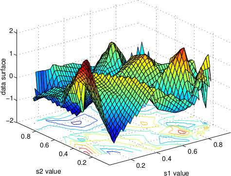
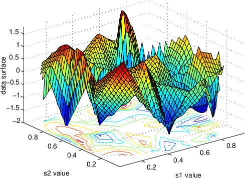
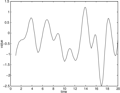
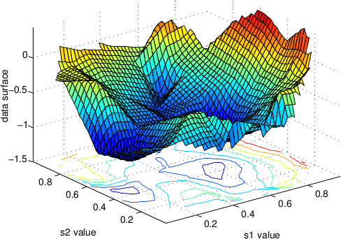
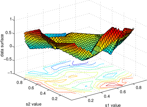
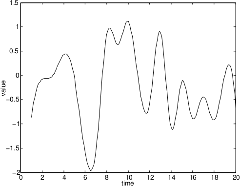
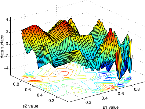
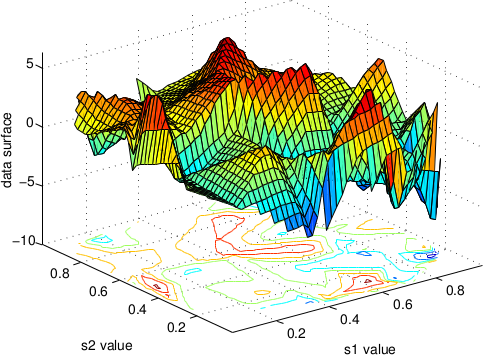
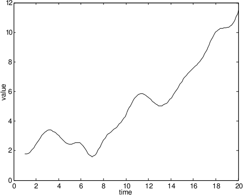
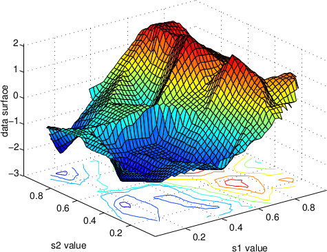
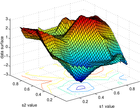
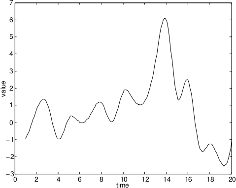
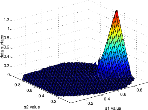
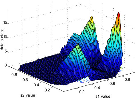
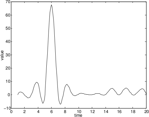
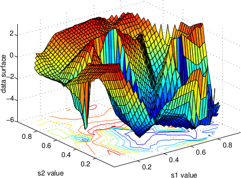
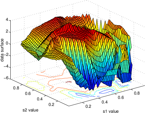
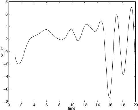
Before delving into a deeper discussion regarding the fitting of the simulated datasets, let us briefly consider the pictures presented in Figure 1. The panels display spatial surfaces and time plots comprising datasets generated by simulation schemes I-IV. The plots in the 1st (leftmost) column show the spatial surfaces obtained by interpolation of the data generated by simulation schemes I to IV for a particular time slice . The plots in the 2nd column show similar spatial surface plots but for a different time slice . The plots in the 3rd (rightmost) column show the time plots obtained by interpolation of the data generated by simulation schemes I to IV for a particular spatial location . For example, panels (a), (b), (c) show the respective spatial surfaces and time plot from simulation scheme I (spatio-temporal white noise). Panels (d), (e), (f), panels (g), (h), (i) and panels (j), (k), (l) show similar spatial surfaces and time plots for simulation schemes II, III and IV, respectively. Note that, the spatial surfaces generated by scheme I (panels (a), (b)) and scheme III (panels (g), (h)) are very jagged and the ones generated by scheme IV (panels (j), (k)) are the smoothest. This is natural as only scheme IV exhibits dependence with respect to both space and time, causing smoothest sample realizations. Regarding the time plots, schemes I (panel (c)) and II (panel (f)) generate very wiggly curves that are strongly indicative of temporal independence, whereas the curve generated by scheme IV (panel (l)) shows smoother behaviour. Scheme III (panel (i)) generates almost a monotonic curve, which hints towards a random walk component.
With datasets generated by the prescribed simulation schemes, now we fit GRFDSTM to them. We also fit the two LDSTMs, discussed above (BGG model and modified-BGG model) and compare their performances with that of the GRFDSTM. Regarding the prior elicitation and fitting of GRFDSTM, we follow the prescription provided in Section 5. Hence, are no longer unknown parameters but some fixed values. Then the unknown parameters associated to the GRFDSTM, that we want to estimate based on the data, comprises the vector parameter associated to the initial process and the parameters associated to the squared exponential covariance kernels as specified in Section 4. We specify independent vague normal priors for each of and specify prior for the parameter vector , where is specified by an isotropic covariance function with scale parameter value and smoothness parameter value . We consider the squared exponential covariance kernels with the following representation . Associated with them we have five covariance kernels , with five scale parameters and five smoothness parameters . Recall that among them are just some fixed quantities. We set and . Fixing the value of to renders the covariance matrix associated with , an identity matrix. This ensures that doesn’t interfere with the spatial dependence structure of . For the rest of the scale and smoothness parameters, we consider independent lognormal priors. For example, we consider lognormal prior for each of the scale parameters and for the data generated by simulation scheme IV. For that same dataset we consider lognormal prior for and lognormal prior for . Note that we use the following representation for the lognormal pdf :
The reason behind choosing very concentrated, almost degenerate priors for and is that, smoothness parameters are notoriously difficult to handle during MCMC computation. Their erratic movement across the Markov chain state space would lead to severely ill-conditioned variance-covariance matrix, making the MCMC algorithm difficult to converge in feasible time. However, with that the question comes how we get these specific priors? In this case lognormal and lognormal respectively. We execute MCMC pilot runs based on a smaller subset of the entire dataset and run the MCMC for different combinations of prior hyper parameters, i.e. we try out lognormal and lognormal and choose the combination of values that gives the best fit in terms of a goodness of fit measure to be introduced later.
So far, we have considered the prior specification regarding the GRFDSTM. Now, let us consider the parameters and prior structures for the BGG model and modified-BGG model. For the BGG model, we follow the same prior structure as prescribed in [5]; vague normal prior for the location parameter , inverse gamma priors for the scale parameters and gamma prior for the smoothness parameter . For the modified-BGG model, the basic structure is exactly the same; however, instead of gamma and inverse gamma, lognormal priors are taken for the scale and smoothness parameters.
To each of the simulated datasets, we fit all the models. We consider iterations of Markov chains for all of them, taking the first iterations as burn-in and the post burn-in iterations have been used for posterior inference. Convergence of the MCMC chains are confirmed by using the CODA package of R. Besides, visual checking of the individual trace-plots also suggests that the convergence is satisfactory.
To assess the model fit we propose a goodness of fit type of statistic. Note that, since the main goal behind developing the GRFDSTM is to predict efficiently, the proposed statistic is so developed to measure how efficiently a model is able to predict at a new spatio-temporal location. Essentially, it is a convex combination of two statistics :
where is any suitable representative central value for the posterior predictive distribution at the spatio-temporal location and is the number of spatio-temporal coordinates , where we are predicting. We recommend using the posterior median as . The statistic measures the deviation of the point prediction value from the observed test data , and measures the width of the Bayesian symmetric prediction interval w.r.t. the posterior predictive distribution . The later part acts like a penalty term, so that any model for which the point prediction value agrees with the observed test data, but the reliability of the point predictor is low, the value of goes up. Hence, even if the test data fall well within the Bayesian symmetric prediction interval; a wider prediction interval means is large and hence the model should be discarded. The amount of penalization is specified by . A natural choice may be . The proposed statistic is essentially a robust version of the predictive criteria for model selection considered in [26].
The findings of the simulation study are summarized in the Table 1.
| Simulation | I. Spatio-tempoal | II. Temporally iid | III. Spatial | IV. Linear | ||
|---|---|---|---|---|---|---|
| schemes | white noise | spatial process | random walk | DSTM | ||
| Percentage | GRFDSTM | 85.20% | 97.40% | 85.90% | 95.40% | |
| of data | BGG model | 96.40% | 100.00% | 100.00% | 99.80% | |
| falling inside | modified-BGG | 95.70% | 99.10% | 94.50% | 99.60% | |
| Bayesian | model | |||||
| symmetric | ||||||
| prediction interval | ||||||
| Bayesian symmetric | GRFDSTM | 3.65 | 0.44 | 14.63 | 1.29 | |
| prediction interval | BGG model | 4.22 | 1.55 | 4.60 | 3.37 | |
| width | modified-BGG | 3.99 | 1.30 | 12.44 | 3.07 | |
| model | ||||||
| Error in | GRFDSTM | 0.99 | 0.08 | 3.79 | 0.25 | |
| Point prediction | BGG model | 0.78 | 0.16 | 0.41 | 0.32 | |
| modified-BGG | 0.78 | 0.19 | 2.35 | 0.40 | ||
| model | ||||||
| Value of | GRFDSTM | 2.32 | 0.26 | 9.21 | 0.77 | |
| statistic | BGG model | 2.50 | 0.85 | 2.50 | 1.85 | |
| modified-BGG | 2.39 | 0.75 | 7.39 | 1.73 | ||
| model |
Following Table 1, we see that for each simulation scheme I-IV, the highest percentage of test data points fall inside the Bayesian symmetric prediction interval given by the BGG model. This is quite likely, given the fact that among the three competing models, the BGG model also produces the widest prediction intervals. The lowest percentage of test data points fall inside the prediction intervals associated with the GRFDSTM, that also produces the narrowest prediction intervals. It is tempting to think that approximately proportion of the test dataset should fall inside the Bayesian symmetric prediction interval, in case the model assumption is adequate. But this consideration is incorrect since firstly, the prediction intervals are calculated based on the univariate posterior predictive distributions for each of the test data points separately and they are highly dependent; more importantly, this is a Bayesian prediction interval and unlike the classical prediction interval a direct relative frequency based interpretation is not available. However, this doesn’t ward off its utility as a model comparison criteria and in general, a model that produces prediction intervals that has moderate widths with many of the test data points lying inside the respective prediction intervals, indicate good performance. Note that, except the spatial random walk scheme, the GRFDSTM performs uniformly better than the two other competing models in terms of the goodness of fit statistic. In particular, for schemes II and IV, where the spatial story is nontrivial, the GRFDSTM performs much better than the BGG model and modified-BGG model. In the case of scheme III, i.e., the spatial random walk case, however, the BGG model performs strikingly better than the GRFDSTM and modified-BGG model. An apparent explanation for that is the inherent random walk structure of the state variables in the BGG model make it the most suitable model for the spatial random walk dataset. The performances of all the three models are very similar in the case of scheme I, that offers no spatial and temporal story. However, as Figure 2 shows, for the simulation schemes I and III, GRFDSTM follows the data pattern much better than the competing two models.
6.2 Simulation from Nonlinear Non-Gaussian Dynamic Spatio-Temporal Models
We have simulated spatio-temporal data using four different linear dynamic models and carried out a comparative study of GRFDSTM and two other LDSTM models on them. The LDSTM models, themselves being linear, show excellent predictive performance. What is more interesting is that the GRFDSTM’s performance is equally competitive. In fact, in schemes II and IV, where there is structured spatial dependence, its performance is better than the BGG model and the modified-BGG model. However, the focal issue behind developing the GRFDSTM is to model nonlinear dynamics efficiently, bypassing the choices of specific nonlinear forms and hence checking its performance when the data is simulated by a nonlinear model, is more crucial. We consider the following two different nonlinear dynamic models and simulate spatio-temporal data using them.
V. Power transform based NLDSTM: This model is motivated by the work of [49] in the context of rainfall modeling. Rainfall is influenced by complex interactions among atmospheric processes and therefore is best modeled by nonlinear models. Similar to the previous simulation schemes, we consider a unit square on and randomly generate spatial locations, where we simulate a single replicate of for using the following spatio-temporal model:
We set aside the data associated with spatial location as test dataset and the rest of the data is fitted using the GRFDSTM and the two other competing LDSTMs (BGG model and modified-BGG model). Here are temporally independent and identically distributed as . The associated variance-covariance matrices and are generated by exponential covariance functions of the form . We choose and . The values of the smoothness parameters are chosen carefully so that there is an interesting spatial story. We choose and , which imply nontrivial temporal evolution. Finally, the value of was set to to make sure that the process exhibits enough nonlinearity within the time span . The observed data is non- Gaussian. However, the nonlinearity in this model is introduced at the observational equation and the state process evolves linearly. The next model, instead, describes a situation where the nonlinearity is expressed through the evolution of the state process.
VI. Threshold NLDSTM: Threshold models are very useful in the context of economic time series data modeling. Spatio-temporal adaptation of such model is described by [8] in the context of forecasting of sea-surface temperature. The grid size and basic design of the simulation remains same as the earlier one, but now we simulate from the following model:
The spatial processes and are temporally independent and identically distributed as centered Gaussian processes with covariance functions and . We choose and .
Like the previous schemes, the data generated by this model is non-Gaussian; indeed a three component Gaussian mixture.
| Simulation | V. Power transform | VI. Threshold | ||||
|---|---|---|---|---|---|---|
| schemes | based NLDSTM | NLDSTM | ||||
| Percentage | GRFDSTM | 90.80% | 94.30% | |||
| of data | BGG model | 97.50% | 98.70% | |||
| falling inside | modified-BGG | 97.50% | 98.20% | |||
| Bayesian | model | |||||
| symmetric | ||||||
| prediction interval | ||||||
| Bayesian symmetric | GRFDSTM | 17.18 | 5.57 | |||
| prediction interval | BGG model | 31.59 | 9.10 | |||
| width | modified-BGG | 26.05 | 9.69 | |||
| model | ||||||
| Error in | GRFDSTM | 4.21 | 1.16 | |||
| Point prediction | BGG model | 3.27 | 1.25 | |||
| modified-BGG | 2.54 | 1.66 | ||||
| model | ||||||
| Value of | GRFDSTM | 10.69 | 3.37 | |||
| statistic | BGG model | 17.43 | 5.18 | |||
| modified-BGG | 14.29 | 5.67 | ||||
| model |
We fit the GRFDSTM and the BGG model and modified-BGG model to the data simulated from the nonlinear non-Gaussian models and the findings are summarized in Table 2. Following Table 2, we see that for both the simulation schemes V and VI, almost the same percentage of test data points fall inside the Bayesian symmetric prediction intervals given by the BGG model and the modified-BGG model. However, the width of the Bayesian symmetric prediction intervals given by the GRFDSTM is much narrower than the intervals given by the two other competing models. In fact, in terms of the goodness of fit statistic, the GRFDSTM demonstrates significantly better performance than the two other competing models. The observations are in keeping with the detailed diagrams depicted in Figure 4, and, as before, it is seen that GRFDSTM follows the data more closely compared to the other competing models.
Comparative study of spatio-temporal models, however, is ambiguous and the result may strongly depend on the details of how the approaches are implemented. Moreover, the choices of the values of the hyper parameters may entirely change the result. [20] also mentioned this issue while comparing two spatio-temporal methods. We do our best to make the comparative study worthwhile in the following way; while the properties associated with the model give us hint about what could be the feasible range of values for different hyper parameters, proposing some fixed values based on them is almost impossible. We use MCMC pilot runs with smaller datasets to find out the values of different hyper parameters. Several different sets of values of hyper parameters were chosen and for each of them, we have MCMC pilot runs based on a smaller subset of the entire dataset. Since, due to smaller sizes of the data sets the pilot runs were much faster, we were able to experiment with many such pilot MCMC runs with different combinations of the hyper parameters. We chose that combination with the smallest value of goodness of fit statistic. Then we performed our final MCMC computations based on the entire dataset using those selected values of the hyper parameters. This strategy is used for selecting the values of hyper parameters associated with each of the three competing models. The models selected by this strategy may not be the best ones, but the strategy provides us with candidate models, based on which a comparative study may be meaningful.
While fitting the GRFDSTM to the simulated datasets we did not have to handle missing data. In reality, however, missing data is quite common in spatio-temporal datasets. Mechanical disturbances and electronic malfunctions in measuring devices may even lead to situations where more than data may be missing at some specific site. Missing data problem, however, can be handled straight forwardly in the GRFDSTM, by the data augmentation technique. The key idea is to treat them as prediction problem.
6.3 Computational Issues
Although dynamic models are preferred over marginal models because of their superior ability to represent the temporal evolution of complex physical processes, they are associated with much higher computational complexities. Modeling of even moderate size spatio-temporal datasets using dynamic spatio-temporal evolution may take significant amounts of time, thus limiting their scope. Even the simplest of LDSTMs may be computationally very demanding owing to handling and inversion of large variance-covariance matrices. It is no wonder, that the problem becomes even more critical in the case of the GRFDSTM. Let us consider the computational cost associated with the GRFDSTM in more detail. Recall that we have monitoring sites where we have collected the data for consecutive time points. Then, in each iteration of the MCMC algorithm for the posterior computation, we need to update the dimensional state vector and the smoothness and scale parameters together using TMCMC, which consist of construction of large covariance matrix, computing their Cholesky decomposition, calculation of the quadratic form and determinants, etc. The total computational cost associated with this step can be shown to be . This total cost is estimated as follows:
| Forming two covariance matrices from | ||
| Cholesky decomposition of the two | ||
Combining them and ignoring all the terms whose total power (adding powers of ) is , we get . Apart from that, we need to update and using Gibbs steps and the total computational complexity associated to that is . Hence, ignoring lower order terms, we obtain the total computational cost for fitting the GRFDSTM to be . However, this is the cost if we use the GRFDSTM just for fitting the data and it increases substantially if we also consider prediction at new locations. Let us assume that we want to predict the whole time series of observations at each of the unmonitored sites. Considering one can show this amounts to the extra cost of the order (ignoring lower order terms). Combining them we get that the total cost of fitting and prediction associated to the GRFDSTM is . Similar calculation for the BGG model (and modified-BGG model) shows that the cost associated with fitting is which is more than the cost associated with fitting GRFDSTM. However, if prediction is considered, the cost associated with BGG model is , which is less compared to the cost of prediction associated with GRFDSTM. Note that, there are one time computations associated with each of these models, which can be safely ignored because of their negligible contributions to the overall computational costs. Besides computing the theoretical complexity, we also investigate the empirical computational time associated with each of the three competing models. Such comparative study of theoretical and empirical computational efficiency is meaningful since the computations associated with all of the three models are implemented through C programs in the same computer. The findings are summarized in Table 3.
| Computational | Computational complexity | Computational cost | Empirical computation |
| procedure | per iteration | per iteration | time (in minutes) taken |
| of MCMC | of MCMC | for MCMC iterations | |
| () | () | ||
| Fitting of GRFDSTM | 9 | ||
| Fitting of BGG model | 18 | ||
| and modified-BGG model | |||
| Prediction | 36 | ||
| by GRFDSTM | |||
| Prediction by BGG model | 19 | ||
| and modified-BGG model |
The empirical computation time is derived based on the spatio-temporal data generated by simulation scheme I, i.e., the spatio-temporal white noise model. All the computations are performed on a standard Dell Inspiron laptop with Intel® Core™ i5-4200U CPU @ 1.60GHz 4 processor. Note that there are differences between the results obtained by theoretical derivation and empirical findings. Such discrepancies are not unexpected given that in reality even inverting two matrices of same order may take different times. Roughly, for the simulation study we have considered, fitting of the GRFDSTM model is twice as fast as that of the BGG model. In the case of prediction, however, the result is reversed and prediction by the BGG model is twice as fast as that of GRFDSTM.
So far, the discussion regarding the computation clearly indicates that the fitting of DSTM models, as well as the GRFDSTM, may be costly. The GRFDSTM works well for small low resolution spatio-temporal dataset. In the following subsection, however we present a simulation study based on a moderate sized spatio-temporal dataset that has been generated by a highly nonlinear sptio-temporal process. Surprisingly, even in this case the GRFDSTM performs very well. That said, however, still the GRFDSTM as it currently specified, is not scalable to large spatio-temporal data i.e. when becomes of the order the computation becomes intractable. For that, one need additional strategies like dimension reduction of the state vector, sparsity assumption regarding the covariance matrices, parallel processing, etc. Indeed, the analysis of massive spatial and spatio-temporal data itself is a rapidly growing area with methods combining ideas from statistics and computer science [4, 6, 14, 15, 16, 23, 36, 41, 58]. In another working paper we are currently trying to develop such a scalable version of the GRFDSTM.
6.4 Moderate Size Spatio-Temporal Data and the GRFDSTM
In this subsection we implement the GRFDSTM to a moderate size dataset, simulated by a highly nonlinear spatio-temporal dynamic model. We generate random locations in and at those spatial locations we generate spatial time series data for according to the following nonlinear spatio-temporal model
where is a spatial variance covariance matrix generated by a squared exponential covariance kernel with smoothness parameter and variance . Once the data is completely generated, then we randomly select spatial locations among the locations and assign them as the test data locations. Hence, the spatial time series data generated at those spatial locations for time is reserved as the test dataset and the rest of the dataset is kept as the training dataset. So, now we have a training dataset of size on which we fit the GRFDSTM and predict the values of the test data. In fact, we gave the whole posterior predictive distribution for each of those test data points. The fit was good and more than of test data are correctly captured in the respective Bayesian symmetric prediction intervals. Below we present some graphs showing the overall performance of the GRFDSTM.
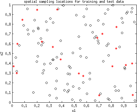
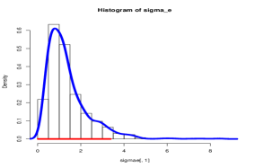
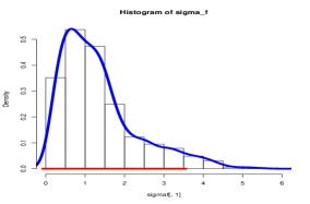
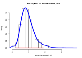
As the above figure suggests, the test data locations are well representative of the training data locations. Regarding the model fitting and prediction we implement the GRFDSTM as specified in Section 4, i.e. we assume that all the covariance kernels are squared exponential type and are fixed. We estimate the rest of the parameters , using an MCMC algorithm. The prior structure is same as Section 5. We take prior for , prior for each of and prior for each of . We consider lognormal prior for each of , lognormal prior for and lognormal prior for . All the priors are independent. The prior hyper parameters are selected based on multiple MCMC pilot runs using a much smaller subset of the whole dataset and then taking the combination of prior hyper parameter values, which gives the best fit. The MCMC runs upto iterations and the first samples were discarded as burn-in samples. Below are some specimen pictures of the MCMC trace plots for some of the parameters. We also present the pictures of posterior distributions (histograms drawn based on the post burn-in samples) of the respective parameters.


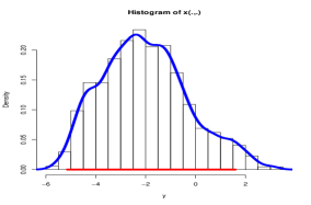
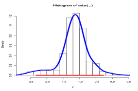
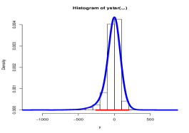
Like the model parameters we also obtain the posterior distributions of the latent variables s associated with the training dataset, the latent variables s associated with the test dataset and the posterior predictive distributions of the observed test data s. Below we present them (in forms of histograms). We also present the trace plots associated with them. Note, that there are a whole bunch of histograms and trace plots each associated with the latent and observed variables at each spatio-temporal coordinate. Here we present the histograms and trace plots associated with the latent and observed variable at particular spatio-temporal coordinate.


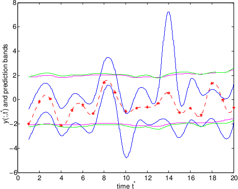
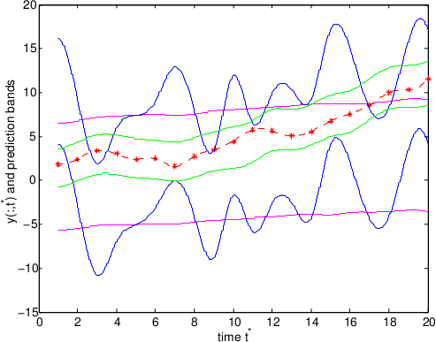
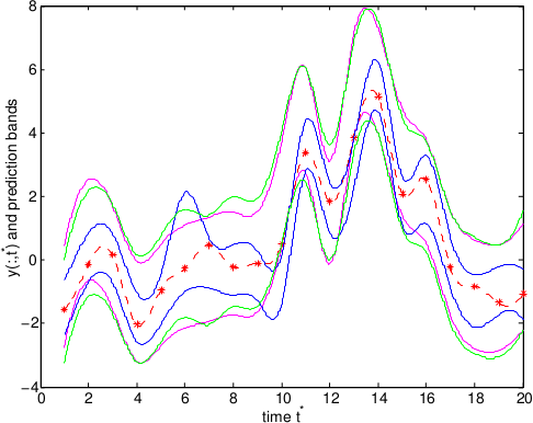
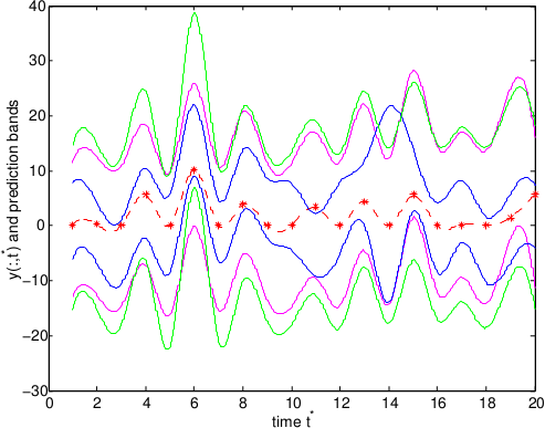
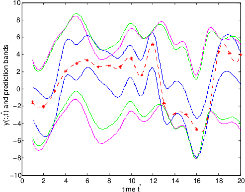
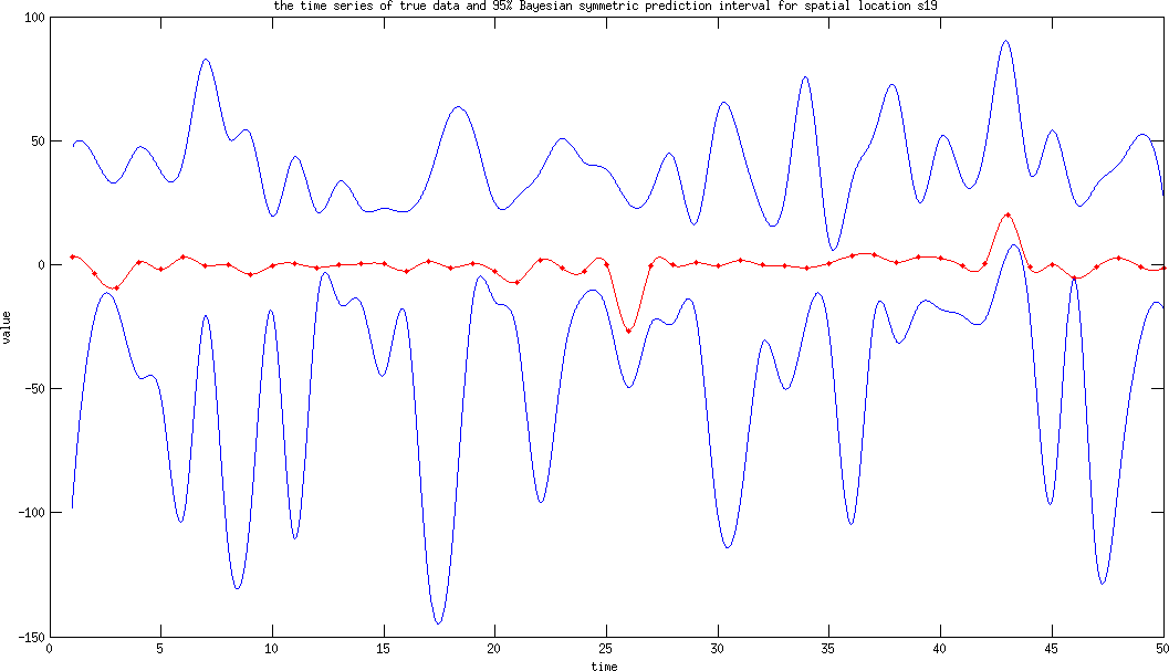
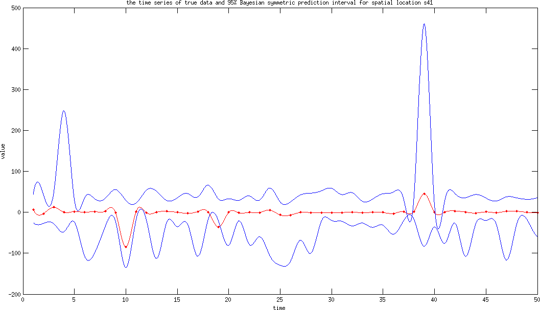
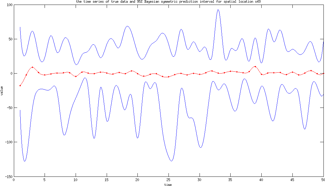
Finally, we present the time series of test data and corresponding Bayesian symmetric prediction band at spatial locations , and . The time series of test data is well within the Bayesian symmetric prediction band at all of the locations. Similar result is observed for other spatial test data locations as well.
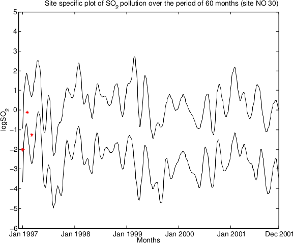
6.5 Realdata Analysis : Pollution over Europe
Air pollution over large geographical regions is a topic of wide range of studies involving statistics and other disciplines. Among them, statistical modeling of pollution caused by draws considerable attention. Here we consider a pollution dataset over Europe. The dataset consists of monthly measurement of sulphur dioxide pollution observed at monitoring stations spread over Europe, for months, starting from January 1997 to December 2001. This dataset is a part of the data collected through the ‘European monitoring and evaluation programme’ (EMEP) which co-ordinates the monitoring of airborne pollution over Europe. Further information is available at http://www.emep.int, and the dataset is freely available there. Simple exploratory analysis reveals the presence of seasonal component and negligible trend component. It is important to note that instead of direct measurement what we have is the measurement of natural logarithm of pollution for these stations.
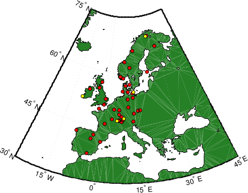
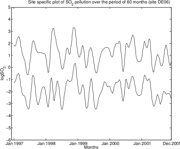
The locations of the sites are shown in Figure 9. Among the monitoring sites, there are sites (yellow circles in Figure 9) where there are large proportions of missing data, making the data associated with those sites highly unreliable. So, we fit the GRFDSTM as specified in Section 5 to the available data and fully reconstruct the pollution time series at those sites. The prior structure used for fitting the GRFDSTM is similar to that of the simulation study. We used diffused bivariate normal priors for and . We consider the squared exponential covariance kernel with the following representation . Associated with five covariance kernels we have five scale parameters and five smoothness parameters . Recall that among them are not really parameters but some fixed entities. For the rest of the scale and smoothness parameters, i.e. , we use independent lognormal priors. As discussed earlier, the lognormal priors associated with are taken to be highly concentrated to avoid ill-conditioning of large covariance matrices, encountered during MCMC computation. The hyper parameters associated with the independent priors are selected based on minimizing goodness of fit statistic over multiple MCMC pilot runs on smaller datasets.
Since the monitoring stations are spread over a large geographical region and distance stretches horizontally as latitude increases, the use of simple longitude and latitude as spatial coordinates would not be appropriate. The Lambert (or Schmidt) projection addresses this problem by preserving the area. This projection is defined by the transformation of longitude and latitude, expressed in radians as and , to the new co-ordinate system . However, with respect to the temporal coordinate we simply take one month as one unit of time.
We implemented an MCMC chain with sufficiently large burn-in (); visual inspection and tests based on CODA package suggests satisfactory convergence. Based on the post burn-in MCMC samples, we calculate the 95% Bayesian symmetric prediction intervals associated with the posterior predictive distributions of at the sites, where we have a large proportion of missing data.
Different scenarios are encountered at those monitoring sites, where we reconstruct the time series. At site , the data is available for the first months of the time period covered. For site , data associated with only the first three months is available. Data is available both at the beginning and at the end of the time period considered, for the site and we don’t have any data for site . Diagrams of the fully reconstructed time series at three monitoring sites are presented in Figure 10.
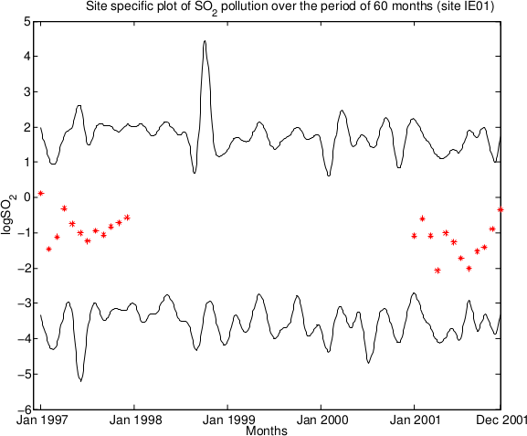
The prediction band corresponding to the monitoring site is much wider and the reconstructed time series at that location is less accurate owing to the fact that its neighbouring stations are quite far away compared to the other sites. Note that in calculating the prediction interval we consider the Bayesian symmetric prediction interval and not the highest posterior density (HPD) interval. The computational cost for HPD is much larger but the gain is little since the spatio-temporal location specific predictive distributions are almost symmetric and there is little difference between Bayesian symmetric prediction interval and the HPD interval.
7 Discussion and Concluding Remarks
Discrete-time spatial time series data often comes with additional covariate information. A simple modification of the GRFDSTM in the following way is capable of handling the covariates
where is the covariate process and is now a Gaussian function on . The rest of the theory remains the same as before. In fact, we can have different covariate processes , in which case will be a Gaussian function on . Note that, for this model, the number of regression parameters in the mean function of the modeled Gaussian process and the number of smoothness parameters increase with the number of covariates, but since the dimensions of the matrices remain unchanged, the computational cost does not increase significantly. Another direction for extension is the time varying version of the GRFDSTM. Such modification is particularly useful when the time interval on which we are observing the data is very wide so that it is unlikely for the functions and to remain invariant with respect to time. In the context of purely temporal state space models, [27] consider time-varying functions and , which they re-write as and , respectively. In other words, they consider the time component as an argument of their random functions and , which are modeled by Gaussian functions in the usual manner. Such ideas can be easily adopted in the GRFDSTM. Currently, we are working on these extensions.
In brief, we recommend using an appropriate NLDSTM model when one clearly knows that the underlying dynamics is nonlinear and also has strong knowledge about the dynamics. The GRFDSTM with possibly nonlinear mean functional associated with and may be considered alternatively, but the performance is generally sub-optimal. However, under no or weak knowledge regarding the dynamics under the spatio-temporal process the GRFDSTM with linear mean functional would exhibit superior predictive performance. The computational cost is more than the prediction by the LDSTMs or NLDSTMs, but the gain is substantial.
Acknowledgments
The research of the first author is fully funded by CSIR SPM Fellowship SPM-07/093(0079)/2010-EMR-I, Govt. of India. We thank ‘European monitoring and evaluation programme’ (EMEP) for the dataset. We are thankful to Moumita Das for many fruitful discussions on this article.
Appendix
Before proving the theorems let us make a notational clarification. The notations and are equivalent and throughout this section they will denote the value of conditional pdf of given at .
Proof of Proposition 3.1.
For this proof we assume that there exist continuous modifications of the Gaussian processes that we consider, that is, there exist processes with sample paths that are continuous everywhere, not just almost everywhere, and that our Gaussian processes equals such processes with probability one (see, for example, see [1] for details). Existence of such continous modifications are guaranteed under the correlation structure that we consider for our Gaussian processes. Note that sometimes the term continuous modification is used in a weaker sense, i.e. to denote a version that is continuous almost everywhere. However, a continuous everywhere version is obtained easily from that by mapping a continuous sample path to itself and a discontinuous sample path to zero function.
Let us first notice that, a probability space such that
where is the space of all real valued continuous functions on and is the Borel sigma field obtained from the topology of compact convergence on the space . Such a joint measurability result need not hold unless and are independent. Now, we will show that is a measurable real valued function or a proper random variable. To show this, first see that can be written as where is a transformation such that, where is a real valued continuous function on and is a real number.
Lemma 7.1.
is a continuous transformation where the topology associated with is the topology of compact convergence and the topology associated with is the usual Euclidean distance based topology on real numbers.
Proof of Lemma 7.1.
Let us consider the metric . This metric induces the
topology of compact convergence on the space . To prove continuity of one needs to show that
and .
Let us assume that and . So, and such that
, .
Now,
and because is continuous.
But,
The RHS goes to as . Hence, . ∎
Once continuity of is proved, note that , for any open set , is an open set in the product topology on the space . Hence, belongs to the Borel sigma field generated by this product topology which is in this case equivalent to the product sigma field associated with . This equivalence holds because both of the spaces and are separable. But is measurable with respect to and . Hence, the inverse image of with respect to is in . So, the inverse image of any open set with respect to is in . This proves the measurability of .
Following exactly same argument as above we can further prove that are jointly measurable. Now, as is independent of and , we have the joint measurability of (See (2)). Infact, we can prove that are jointly measurable. To do it we consider such that where is a real valued continuous function on and is a real number. Then similarly as in case of we can prove that is also a continuous map which immediately implies that are jointly measurable. Then being independent of and , implies the joint measurability of . Hence, starting with the joint measurability of we prove the joint measurability of and . Similarly, if we start with joint measurability of we can prove the joint measurability of . Thus, the joint measurability of the whole collection of state variables is mathematically established.
Now, to prove joint measurability of the collection of observed variables recall the observational equation (1). Since, takes values in just as , and also since is independent of just as is independent of , all the previous arguments go through in this case and joint measurability of is established.
Finally, it remains to show that a valid spatio-temporal process is induced by this model. But it is immediate from the application of Kolmogorov consistency theorem. The consistency conditions of the theorem are trivially satisfied by our construction and hence the result follows. ∎
Alternative proof of Proposition 3.1.
In the previous proof, we need to assume the existence of continuous modification of the underlying Gaussian processes. Here we present an alternative proof, which is lengthier, but remains valid even if the underlying Gaussian processes do not admit a continuous modification. In fact, the alternative proof go through if the underlying process admits at most countable number of discontinuities and hence might be of independent interest in the study of iterated random functions.
Note that it is possible to represent any stochastic process , for fixed as a random variable , where ; being the set of all functions from into . Also, fixing , the function , represents a path of . Indeed, we can identify with the function from to ; see, for example, [40], for a lucid discussion. This latter identification will be convenient for our purpose, and we adopt this for proving our result on measurability.
Note that the -algebra induced by is generated by sets of the form
where , are Borel sets in .
In our case, the Gaussian process can be identified with , for any fixed and , where is the set of all functions from to . The initial Gaussian process can be identified with , where (although, we develop the GRFDSTM assuming this proof is given under the more general setting of ) and . Here is the set of all functions from to . Let and be the Borel -fields associated with and , respectively.
We first show that the composition of with , given by is a measurable random variable for any . Since and are independent, we need to consider the product space , and noting that , where , need to show that sets of the form
where , are Borel sets in , are in , the product Borel -field associated with . For our purpose, we let be of the form for real values .
Now, suppose that . Then , which implies that is at most a countable union of sets of the form , where is a countable set of indices. Also, it holds that . Here is the countable set of rationals in . If necessary, we can envisage a countable set consisting of points of discontinuities of . If is a point of discontinuity, then may be only the left limit of particular sequence or only the right limit of a particular sequence , or may be an isolated point, not reachable by sequences of the above forms. It follows that must lie in
Now, if , then, noting that for any point of , , where , it is easily seen that . Hence, .
Now observe that is a finite intersection of countable union of measurable sets; hence, is itself a measurable set. In other words, we have proved that is measurable. Now, as is independent of and , it follows from (2) that is measurable.
To prove measurability of , note that
| (7) |
The process requires introduction an extra sample space , so that we can identify as . With this, we can represent of (7) as .
Now, implies that . If for some , then the set of solutions is
| (8) |
where implies, as before, that belongs to a countable union of measurable sets in . Although the set (8) is an uncountable union, following the technique used for proving measurability of , we will intersect the set by , the (countable) set of rationals in ; this will render the intersection a countable set. The proof of measurability then follows similarly as before.
Proceeding likewise, we can prove measurability of is measurable for . Proceeding exactly in the same way, we can also prove that are measurable. Moreover, it can be easily seen that the same methods employed for proving the above results on measurability can be extended in a straightforward (albeit notationally cumbersome) manner to prove that the sets of the forms
are also measurable. Furthermore, it can be easily verified that and satisfy Kolmogorov’s consistency criteria. In other words, and are well-defined stochastic processes in both space and time. ∎
Proof of Theorem 3.2.
Let us first observe that conditional on our latent process satisfies the Markov property. That is,
where denotes the conditional density of at given . Now, let us represent by for all and . Then repeatedly using the Markov property we have following
But, this is the joint density of the state variables conditioned on . To obtain the joint density of the state variables one needs to marginalize it with respect to the Gaussian process . After marginalization, the joint density takes the following form:
where is as in (3.2). This is nothing but a convolution of two dimensional Gaussian densities, one with mean vector
and covariance matrix and the other one with mean vector
and covariance matrix .
Hence, the integral boils down to
where is as in (3.2). ∎
Proof of Theorem 3.3.
First, see that for fixed , is distributed as a Gaussian with mean and variance where and are respectively the process variance associated with the isotropic Gaussian processes and (see (3) and (1)). Now, see that for fixed and , and has covariance . Also, and are mutually independent spatial Gaussian processes for . Hence, conditional on state variables the covariance between and is . Here is the delta function i.e. for and otherwise.
So, the joint density of the observed variables, which is denoted by , is given by
Hence, part follows.
For part note that if , the conditional density
is Gaussian with block diagonal covariance matrix . On the other hand,
we have already noted that if , the joint density of the state variables boils down to Gaussian
(see the discussion following Theorem 3.2). Let us consider only the state variables from time onwards.
They jointly follow an dimensional Gaussian distribution. It is not difficult to see that the mean vector and the covariance matrix
of the dimensional Gaussian distribution are of following forms:
the th entry of the mean vector is where
and the th entry of the covariance matrix is
where and
is the th entry of the covariance matrix .
Now, using part we see that the joint distribution of is nothing but
a convolution of two -dimensional Gaussian densities. Hence, it is a Gaussian distribution whose mean vector
has th entry as and the th entry of the covariance matrix is
where and . So, part is proved.
∎
Proof of Theorem 3.4.
To prove part , we first show that is finite. Then by using the formula
we establish that is finite that in turn implies that is finite.
To show is finite we use principle of mathematical induction, i.e. we first show that is
finite and then we show that if
are finite
then is finite. These two steps together compel to be finite for all and .
The first step is trivially shown as is a Gaussian random variable.
Now we show the second step of mathematical induction, that is, we show that if
are finite then is finite.
Let us consider the following:
where is the row vector
and is the variance covarince matrix induced by covariance function .
Now, we consider .
We want to show that this quantity is finite. But the problem is that we have to deal with the inverse of a random matrix
. Fortunately,
the random matrix is non-negative definite (nnd). Hence,
. On the other hand, this quantity being a conditional variance is always nonnegative.
So, the following inequality holds
Hence, it follows that
So, the quantity being equivalent to , is finite.
Now we consider the term .
where is the row vector . We want to show that is finite. Equivalently, we want to show is finite. For that it is enough to show is finite since our induction hypothesis already assume that is finite.
Now we show that is finite. First note that can be expressed as a linear combination of the elements of as . If the are fixed numbers it is easy to see that has finite second moment. Unfortunately, are random. However we will show that they are bounded random variables and then using a lemma we will prove that is finite.
First we show that are bounded random variables. Consider the spectral decomposition of the real symmetric (nnd) matrix . Let us assume that , where is an orthogonal matrix and is the diagonal matrix whose diagonal elements are eigenvalues. Then
Since is a (random) orthogonal matrix its elements are bounded random variables between and . The (random) elements of the row vector are covariances induced by the isotropic covariance kernel . Hence, they are bounded random variables between and . Finally, the (random) elements of are bounded random variables between and . Hence, the (random) row vector , being a product of some random matrices whose elements are bounded random variables, is itself composed of bounded random variables. So, its elements , although random, are bounded. Now, we state a crucial lemma.
Lemma 7.2.
Let us assume that are random variables with finite second moment and are bounded random variables all defined on same probability space. Then the random variables also has finite second moment.
Proof.
Let us assume that lie between and for . Now . But . So, .
So,
So, has finite second moment.
∎
Once we apply the lemma to the finiteness of is immediate. Then by the formula we get that is finite. ∎
We now prove part . Since we have already proved in part that the coordinate variables of the observed spatio-temporal process have finite variances, now we can consider the covariance function associated with the process and study its properties. Let us denote the covariance between and by . Then
Now, the term will be nonstationary and hence . In fact, with probability 1 because has density with respect to Lebesgue measure and this heuristically justifies our argument. So, the covariance function is nonstationary in both space and time.
To prove non separability, first see that is non separable in space and time, because both space and time are involved in it through . Hence, is nonseparable and therefore is nonseparable in space and time.
Proof of Theorem 3.5.
First consider where WLOG we assume . Also, assume that is the centered Gaussian process obtained from . Then
Repeatedly expanding the term in the same way we get
| (10) | |||
Just as the previous paragraph we can further see that
| (11) |
Now we plan to show that terms of the types and are negligible if is small enough. Our next lemma proves it rigorously.
Lemma 7.3.
For arbitrarily small , such that for .
See that it is enough to prove that is arbitrarily small . Then Cauchy-Schwartz inequality implies is arbitrarily small. Similarly, Cauchy-Schwartz inequality implies is arbitrarily small. Then we are done by the expansion
Before proceeding towards the proof we mention two results from Gaussian process (see [1] for details) that will be used subsequently.
Result 7.4 (Borell-TIS inequality).
Let us assume that is an almost surely bounded centered Gaussian process on index set
. Define .
Then for where .
Result 7.5 (Dudley’s metric entropy bound).
Under the assumption of the Borel-TIS inequality,
,
where is the diameter of the index set with respect to the canonical pseudo-metric associated with the Gaussian process given by , and where is the minimum number of balls required to cover the index set with respect to the canonical pseudo-metric ; is a universal constant.
With the above two results, we are ready to prove Lemma 7.3.
Proof of Lemma 7.3.
Consider . Observe that
Now, using the change of variable the integral can be reduced to the form
Hence, .
But, by Result 7.5
and it is not difficult to see that is a decreasing function of . The same is true of
when as a function of . These two facts together permit applicability of the monotone convergence theorem to yield
So, which in turn implies can be made arbitrarily small by making small. This proves Lemma 7.3. ∎
Arguing similarly one can also show that for arbitrarily small , such that for . Moreover, see that the bound is uniform in and . Since , using the bound repeatedly in (15), we obtain
Similarly, using the bound repeatedly in (16), we obtain
Combining them we get
Now plugging in this approximation in the expression for we get the desired result. So, Theorem 3.5 is finally proved.
∎
Proof of Theorem 3.6.
Part : Arguing in the similar lines as in the proof of Proposition 3.1, one can show that a probability space such that for , are continuous functions in where and are continuous functions in . Then by the property of composition of two functions is a continuous function in . Proceeding recursively, one can prove that is a continuous function in for any . Once we show is a continuous function, we prove is a continuous function in . So, part is proved.
Part : Proof of part is similar to that of part . Firstly, we state a simple lemma.
Lemma 7.6.
Let us consider two real valued functions and such that both of them are times differentiable. Then the composition function is also times differentiable.
Proof.
Proof of this lemma is basically a generalization of chain rule for multivariate functions and can be found in advanced multivariate calculus text books. We give a brief sketch of the proof. First we clarify the term times differentiable for the function . It means all mixed partial derivatives of of order exist. We prove the lemma using mathematical induction. Firstly, We show that the lemma is true for and then we show that if the lemma is true for then it must be true for as well.
That the lemma is true for easily follows from the chain rule for multivariate functions. Now we prove the second step. By the induction hypothesis the lemma is true for the case and and are times differentiable. We want to show that is also times differentiable. Without loss of generality, we consider the mixed partial derivative where and show that it exists. Observe that the partial derivative is equivalent to provided it exists. Since, by the induction hypothesis the lemma is true for the case and and are times differentiable, the composition of them is also times differentiable. On the other hand, is also times differentiable. So, the product of them is also times differentiable. Hence the partial derivative exists. Equivalently, exists. Similarly one can prove the existence of other mixed partial derivatives of of order . Hence, by induction the proof follows. ∎
Part : From the condition of the theorem it is clear that a probability space such that for , are times differentiable functions in where and are times differentiable functions in . Then by the above lemma is a times differentiable function in . The rest of the proof is exactly similar as in part .
∎
Proof of Propositon 4.1.
where is the matrix associated with parameter value and . is the pdf
associated with parameter value . Similarly the pdf is denoted by
where is the matrix associated with parameter value and . is the pdf
associated with parameter value .
Now recall that is given by
where is the matrix associated with associated with parameter value and . Similarly, we may define as the matrix associated with associated with parameter value and . Then, it is easy to see that , and that in turn implies .
Hence,
.
∎
Proof of Theorem 4.2.
Assume . We want to show . Since, in this case are fixed so it is enough to show .
From the proof of part (a) of Theorem 3.3 we get that for fixed , is distributed as a Gaussian with mean . Hence, . Now, put to get . But, . Combining these results we get
| (12) |
Again from the proof of part (a) of Theorem 3.3 we get that where is the delta function i.e. for and otherwise. Since, by assumptions of the Theorem 4.2 all the covariance kernels are squared exponential type this expression becomes . Now, put to get . Hence,
Now,
Combining these results we get
| (13) |
Now, see that implies . Hence, by equation (12)
| (14) |
Similarly, noting that the term remains same under and ; implies (by equation (13))
| (15) |
Now we, solve equation (14) and (15) to show that . Note that, equation (15) can be represented as where and . Then by assumption (C) such that
| (16) | ||||
| (17) | ||||
| (18) |
WLOG we assume . There are three possibilities, i.e. , and .
Case I: Assume . Then equation (16) . Now, using equation (17) we get that
(since by the assumption ). So, . Now, . Moreover, using in equation (16) .
Case II: Assume . We show it leads to contradiction. Since, by assumption and , the case II can be exhaustively represented by sub cases; sub case IIa : , sub case IIb : and sub case IIc : .
Subcase IIa: If then see that ; contradiction. Or, if ; then . Hence, implies . Then by Jensen’s inequality, ; contradiction.
Subcase IIb: If then see that ; contradiction. Or, if ; then . Hence, implies . Then again by Jensen’s inequality, we get contradiction.
Subcase IIc: If then see that ; contradiction. Or, if ; then ; contradiction.
Case III: Assume . Now, we put in place of and then symmetry and subcase IIb leads to contradiction.
With that we establish that must be and and .
Now we show that leads to contradiction implying . We substitute in equation (14) to get i.e. ; contradiction since by assumption (C) of Theorem 4.2 at least one pair such that . So, . Now, we replace that in equation (14) and get which implies .
∎
References
- [1] ADLER, R. J. and TAYLOR, J. E. (2007). Random Fields and Geometry. Springer. ISBN-13: 978-0-387-48112-8.
- [2] AMINI, H. et al. (2016). Annual and seasonal spatial models for nitrogen oxides in Tehran, Iran. Sci. Rep., 6: 32970, 2016. ISSN 2045-2322. doi: 10.1038/srep32970. URL https://www.nature.com/articles/srep32970.pdf.
- [3] BANERJEE, S., CARLIN, B. P. and GELFAND, A. (2004). Hierarchical Modeling and Analysis for Spatial Data. Chapman & Hall/CRC. ISBN 1-58488-410-X.
- [4] BANERJEE, S. (2017). High-Dimensional Bayesian Geostatistics. Bayesian Anal., 12(2): 583-614, 2017. ISSN 1931-6690. doi: 10.1214/17-BA1056R. URL http://projecteuclid.org/euclid.ba/1494921642.
- [5] BANERJEE, S., GAMERMAN, D. and GELFAND, A. E. (2005). Spatial process modelling for univariate and multivariate dynamic spatial data. Environmetrics, 16(5): 465-479, 2005. ISSN 1099-095X. doi: 10.1002/env.715. URL http://onlinelibrary.wiley.com/doi/10.1002/env.715/pdf.
- [6] BANERJEE, S., GELFAND, A. E., FINLEY, A. O. and SANG, H. (2008). Gaussian predictive process models for large spatial data sets. J. Roy. Statist. Soc. Ser. B, 70(4): 825–848, 2008. ISSN 1467-9868. doi: 10.1111/j.1467-9868.2008.00663.x. URL http://onlinelibrary.wiley.com/doi/10.1111/j.1467-9868.2008.00663.x/pdf.
- [7] BERLINER, L. M., MILLIFF, R. F. and WIKLE, C. (2003). Bayesian hierarchical modeling of air-sea interaction. J. Geophys. Res., 108(C4): 2003. ISSN 2169-9291. doi: 10.1029/2002JC001413. URL http://onlinelibrary.wiley.com/doi/10.1029/2002JC001413/epdf.
- [8] BERLINER, L. M., WIKLE, C. and CRESSIE, N. (2000). Long-Lead Prediction of Pacific SSTs via Bayesian Dynamic Modeling. Journal of Climate, 13(22): 3953-3968, 2000. ISSN 1520-0442. doi: http://dx.doi.org/10.1175/1520-0442(2001)013¡3953:LLPOPS¿2.0.CO;2. URL http://journals.ametsoc.org/doi/full/10.1175/1520-0442%282001%29013%3C3953%3ALLPOPS%3E2.0.CO%3B2.
- [9] BLOOMFIELD, P., OEHLERT, G., THOMPSON, M. L. and ZEGER, S. (1983). A frequency domain analysis of trends in Dobson total ozone records. J. Geophys. Res., 88(C13): 8512–8522, 1983. ISSN 2169-9291. doi: 10.1029/JC088iC13p08512. URL http://onlinelibrary.wiley.com/doi/10.1029/JC088iC13p08512/abstract.
- [10] BRUNO, F., GUTTORP, P., SAMPSON, P. D. and COCCHI, D. (2009). A simple non-separable, non-stationary spatiotemporal model for ozone. Environ. Ecol. Stat., 16(4): 515-529, 2009. ISSN 1573-3009. doi: 10.1007/s10651-008-0094-8. URL http://link.springer.com/article/10.1007/s10651-008-0094-8.
- [11] CHAKRABORTY, A. et al. (2010). Modeling large scale species abundance with latent spatial processes. Ann. Appl. Stat., 4(3): 1403-1429, 2010. ISSN 1932-6157. doi: doi:10.1214/10-AOAS335. URL https://projecteuclid.org/euclid.aoas/1287409379.
- [12] COX, D. R. and ISHAM, V. (1988). A Simple Spatial-Temporal Model of Rainfall. Proc. R. Soc. Lon. Ser. A, 415(1849): 317-328, 1988. ISSN 1471-2946. URL http://www.jstor.org/stable/2398094.
- [13] CRESSIE, N. and WIKLE, C. K. (2011). Statistics for Spatio-Temporal Data.. Wiley. ISBN 978-0-471-69274-4.
- [14] CRESSIE, N. and JOHANNESSON, G. (2008). Fixed rank kriging for very large spatial data sets. J. Roy. Statist. Soc. Ser. B, 70(1): 209–226, 2008. ISSN 1467-9868. doi: 10.1111/j.1467-9868.2007.00633.x. URL http://onlinelibrary.wiley.com/doi/10.1111/j.1467-9868.2007.00633.x/pdf.
- [15] DATTA, A., BANERJEE, S., FINLEY, A. O. and GELFAND, A. E. (2016). Hierarchical Nearest-Neighbor Gaussian Process Models for Large Geostatistical Datasets. J. Amer. Statist. Assoc., 111(514): 800-812, 2016. ISSN 1537-274X. doi: 10.1080/01621459.2015.1044091. URL http://dx.doi.org/10.1080/01621459.2015.1044091.
- [16] DATTA, A. et al. (2016). Nonseparable dynamic nearest neighbor Gaussian process models for large spatio-temporal data with an application to particulate matter analysis. Ann. Appl. Stat., 10(3): 1286-1316, 2016. ISSN 1932-6157. doi: 10.1214/16-AOAS931. URL http://projecteuclid.org/euclid.aoas/1475069608.
- [17] DENG, J. S., WANG, K., HONG, Y. and QI, J. G. (2009). Spatio-temporal dynamics and evolution of land use change and landscape pattern in response to rapid urbanization. Landscape. Urban. Plan., 92(3): 187-198, 2009. ISSN 0169-2046. doi: https://doi.org/10.1016/j.landurbplan.2009.05.001. URL http://www.sciencedirect.com/science/article/pii/S0169204609000814.
- [18] DEY, K., K., and BHATTACHARYA, S. (2016a). On Optimal Scaling of Additive Transformation Based Markov Chain Monte Carlo. URL http://arxiv.org/abs/1307.1446.
- [19] DEY, K., K., and BHATTACHARYA, S. (2016b). On Geometric Ergodicity of Additive and Multiplicative Transformation Based Markov Chain Monte Carlo in High Dimensions. Forthcoming in Brazilian Journal of Probability and Statistics URL http://imstat.org/bjps/papers/BJPS295.pdf.
- [20] DOU, Y., LE, N. D. and ZIDEK, V. (2010). Modeling hourly ozone concentration fields. Ann. Appl. Stat., 4(3): 1183-1213, 2010. ISSN 1932-6157. doi: 10.1214/09-AOAS318. URL http://projecteuclid.org/DPubS/Repository/1.0/Disseminate?view=body&id=pdfview_1&handle=euclid.aoas/1287409369.
- [21] DUTTA, S. and BHATTACHARYA, S. (2014). Markov chain monte carlo based on deterministic transformations. Statistical Methodology, 16: 100-116, 2014. ISSN 1572-3127. URL http://www.sciencedirect.com/science/article/pii/S1572312713000683.
- [22] FONSECA, T. C. O. and STEEL, M. F. J. (2011). Non-Gaussian spatiotemporal modelling through scale mixing. Biometrika, 98(4): 761-774, 2011. ISSN 1464-3510. doi: 10.1093/biomet/asr047. URL http://biomet.oxfordjournals.org/content/98/4/761.abstract.
- [23] FURRER, R. and SAIN, S. R. (2009). Spatial model fitting for large datasets with applications to climate and microarray problems. Stat. Comput., 19(2): 113-128, 2009. ISSN 1573-1375. doi: 10.1007/s11222-008-9075-x. URL http://www.springerlink.com/content/203124p861356383/.
- [24] GELFAND, A. E., ECKER, M. D., KNIGHT, J. R. and SIRMANS, C. F. (2004). The Dynamics of Location in Home Price. J. Real. Estate. Financ., 29(2): 149–166, 2004. ISSN 0895-5638. doi: 10.1023/B:REAL.0000035308.15346.0a. URL http://link.springer.com/article/10.1023/B:REAL.0000035308.15346.0a.
- [25] GELFAND, A. E., DIGGLE, P. J., FUENTES, M., and GUTTORP, P. (2010). Handbook of Spatial Statistics. CRC Press. ISBN 978-1-4200-7287-7. URL http://www.crcpress.com/product/isbn/9781420072877.
- [26] GELFAND, A. E. and GHOSH, S. K. (1998). Model choice: A minimum posterior predictive loss approach. Biometrika, 85(1): 1-11, 1998. ISSN 1464-3510. doi: doi:10.1093/biomet/85.1.1. URL http://biomet.oxfordjournals.org/content/85/1/1.full.pdf+html.
- [27] GHOSH, A., MUKHOPADHYAY, S., ROY, S., and BHATTACHARYA, S. (2014). Bayesian Inference in Nonparametric Dynamic State-Space Models. Statistical Methodology, 21: 35-48, 2014. doi: http://dx.doi.org/10.1016/j.stamet.2014.02.004. URL http://www.sciencedirect.com/science/article/pii/S1572312714000197.
- [28] GIANNITRAPANI, M., BOWMAN, A. SCOTT, M., and SMITH, R. (2006). Sulphur dioxide in Europe: Statistical relationships between emissions and measured concentrations. Atmos. Environ. , 40(14): 2524-2532, 2006. ISSN 1352-2310. doi: 10.1016/j.atmosenv.2005.12.052. URL http://www.sciencedirect.com/science/article/pii/S1352231006000070.
- [29] GUTTORP, P., MEIRING, W. and SAMPSON, P. D. (1994). A space-time analysis of ground-level ozone data. Environmetrics, 5(3): 241-254, 1994. ISSN 1099-095X. doi: 10.1002/env.3170050305. URL http://onlinelibrary.wiley.com/doi/10.1002/env.3170050305/pdf.
- [30] HOLLAND, D. M., OLIVEIRA, V. D., COX, L. H. and SMITH, R. L. (2000). Estimation of regional trends in sulfur dioxide over the eastern United States. Environmetrics, 11(4): 373-393, 2000. ISSN 1099-095X. doi: 10.1002/1099-095X(200007/08)11:4¡373::AID-ENV419¿3.0.CO;2-2. URL 10.1002/1099-095X(200007/08)11:4<373::AID-ENV419>3.0.CO;2-2.
- [31] HOOTEN, M. B. and WIKLE, C. K. (2007). Shifts in the spatio-temporal growth dynamics of shortleaf pine. Environ. Ecol. Stat., 14(3): , 2007. ISSN 1352-8505 . doi: 10.1007/s10651-007-0016-1. URL http://link.springer.com/article/10.1007/s10651-007-0016-1.
- [32] HUANG, H. H. and CRESSIE, N. (1996). Spatio-temporal prediction of snow water equivalent using the Kalman filter. Comput. Stat. Data. An., 22(2): 159-175, 1996. ISSN 0167-9473. doi: 10.1016/0167-9473(95)00047-X. URL http://www.sciencedirect.com/science/article/pii/016794739500047X.
- [33] HUERTA, G., SANSÓ, B. and STROUD, J. R. (2004)). A spatiotemporal model for Mexico City ozone levels. Appl. Statist., 53(2): 231-248, 2004. ISSN 1467-9876. doi: 10.1046/j.1467-9876.2003.05100.x. URL http://onlinelibrary.wiley.com/doi/10.1046/j.1467-9876.2003.05100.x/pdf.
- [34] HUGHES, J. P. and GUTTORP, P. (1994). A class of stochastic models for relating synoptic atmospheric patterns to regional hydrologic phenomena. Water. Resour. Res., 30(5): 1535-1546, 1994. ISSN 1944-7973. doi: 10.1029/93WR02983. URL http://onlinelibrary.wiley.com/doi/10.1029/93WR02983/pdf.
- [35] JUN, M., KNUTTI, R. and NYCHKA, D. W. (2008). Spatial analysis to quantify numerical model bias and dependence: How many climate models are there? J. Amer. Statist. Assoc., 103(483): 934-947, 2008. ISSN 1537-274X. doi: 10.1198/016214507000001265. URL http://www.tandfonline.com/doi/abs/10.1198/016214507000001265.
- [36] KAUFMAN, C. G., SCHERVISH, M. J. and NYCHKA, D. (2008). Covariance Tapering for Likelihood-Based Estimation in Large Spatial Data Sets. J. Amer. Statist. Assoc., 103(484): 1545-1555, 2008. ISSN 1537-274X. doi: 10.1198/016214508000000959. URL http://amstat.tandfonline.com/doi/abs/10.1198/016214508000000959.
- [37] KNIGHT, J. R., DOMBROW, J. and SIRMANS, C. F. (1995). A Varying Parameters Approach to Constructing House Price Indexes. Real. Estate. Econ., 23(2): 187–205, 1995. ISSN 1540-6229. doi: 10.1111/1540-6229.00663. URL http://onlinelibrary.wiley.com/doi/10.1111/1540-6229.00663/abstract.
- [38] LOPES, H. F., SALAZAR, E. and GAMERMAN, D. (2008). Spatial Dynamic Factor Analysis. Bayesian Anal., 3(4): 759-792, 2008. ISSN 1931-6690. doi: 10.1214/08-BA329. URL https://projecteuclid.org/euclid.ba/1340370408.
- [39] MARDIA, K. V., GOODALL, C., REDFERN, E. J. and ALONSO, F. J. (1998). The Kriged Kalman filter. Test, 7(2): 217–282, 1998. ISSN 1133-0686. doi: 10.1007/BF02565111. URL http://link.springer.com/article/10.1007/BF02565111.
- [40] ØKSENDAL, B. (2000). Stochastic Differential Equations. 5th Edition. Springer-Verlag. Hiedelberg, New York.
- [41] PACIOREK, C. J. et al. (2009). Practical large-scale spatio-temporal modeling of particulate matter concentrations. Ann. Appl. Stat., 3(1): 370-397, 2009. ISSN 1932-6157. doi: 10.1214/08-AOAS204. URL https://projecteuclid.org/download/pdfview_1/euclid.aoas/1239888375.
- [42] PAEZ, M. S., GAMERMAN, D., LANDIM, F. M. P. F. and SALAZAR, E. (2008). Spatially varying dynamic coefficient models. J. Stat. Plan. Infer., 138(4): 1038–1058, 2008. ISSN 0378-3758. doi: 10.1016/j.jspi.2007.03.060. URL http://www.sciencedirect.com/science/article/pii/S0378375807002650.
- [43] PALACIOS, M. B. and STEEL, M. F. J. (2006). Non-Gaussian Bayesian Geostatistical Modeling. J. Amer. Statist. Assoc., 101(474): 604-618, 2006. ISSN 1537-274X. doi: 10.1198/016214505000001195. URL http://www.tandfonline.com/doi/abs/10.1198/016214505000001195#.UjrXM0nJXQo.
- [44] RASMUSSEN, C. E. and WILLIAMS, C. K. I. (2006). Gaussian Processes for Machine Learning. MIT Press. ISBN 0-262-18253-X.
- [45] REINSEL, G. et al. (1967). Statistical analysis of stratospheric ozone data for the detection of trends. Atmos. Environ. , 15(9): 1569-1577, 1967. ISSN 1352-2310. doi: 10.1016/0004-6981(81)90140-2. URL http://www.sciencedirect.com/science/article/pii/0004698181901402.
- [46] SAHU, S. K., GELFAND, A. E. and HOLLAND, D. M. (2010). Fusing point and areal level space–time data with application to wet deposition. J. Roy. Statist. Soc. Ser. C, 59(1): 77–103, 2010. ISSN 1467-9876. doi: 10.1111/j.1467-9876.2009.00685.x. URL http://onlinelibrary.wiley.com/doi/10.1111/j.1467-9876.2009.00685.x/abstract.
- [47] SAIN, S. R., FURRER, R. and CRESSIE, N. (2011). A spatial analysis of multivariate output from regional climate models. Ann. Appl. Stat., 5(1): 150-175, 2011. ISSN 1932-6157. doi: 10.1214/10-AOAS369. URL http://projecteuclid.org/DPubS?service=UI&version=1.0&verb=Display&handle=euclid.aoas/1300715186.
- [48] SANG, H., JUN, M. and HUANG, J. Z. (2011). Covariance approximation for large multivariate spatial data sets with an application to multiple climate model errors. Ann. Appl. Stat., 5(4): 2519-2548, 2011. ISSN 1932-6157. doi: 10.1214/11-AOAS478. URL http://projecteuclid.org/DPubS?service=UI&version=1.0&verb=Display&handle=euclid.aoas/1324399605.
- [49] SANSÓ, B. and GUENNI, L. (1999). Venezuelan rainfall data analysed by using a Bayesian space–time model. J. Roy. Statist. Soc. Ser. C, 48(3): 345-362, 1999. ISSN 1467-9876. doi: 10.1111/1467-9876.00157. URL http://onlinelibrary.wiley.com/doi/10.1111/1467-9876.00157/pdf.
- [50] SANSÓ, B., SCHMIDT, A. M. and NOBRE, A. A. (2008). Bayesian spatio-temporal models based on discrete convolutions. Can. J. Stat., 36(2): 239-258, 2008. ISSN 1708-945X. doi: 10.1002/cjs.5550360205. URL http://onlinelibrary.wiley.com/doi/10.1002/cjs.5550360205/pdf.
- [51] SMITH, R. L., TEBALDI, C., NYCHKA, D. and MEARNS, L. O. (2009). Bayesian modeling of uncertainty in ensembles of climate models. J. Amer. Statist. Assoc., 104(485): 97-116, 2009. ISSN 1537-274X. doi: 10.1198/jasa.2009.0007. URL http://amstat.tandfonline.com/doi/abs/10.1198/jasa.2009.0007.
- [52] STORVIK, G., FRIGESSI, A. and HIRST, D. (2002). Stationary space-time Gaussian fields and their time autoregressive representation. Statistical Modelling, 2(2): 139-161, 2002. ISSN 1471-082X. doi: 10.1191/1471082x02st029oa. URL http://smj.sagepub.com/content/2/2/139.full.pdf+html.
- [53] STROUD, J. R., MÜLLER, P. and SANSÓ, B. (2001). Dynamic models for spatiotemporal data. J. Roy. Statist. Soc. Ser. B, 63(4): 673-689, 2001 . ISSN 1467-9868. doi: 10.1111/1467-9868.00305. URL http://www.jstor.org/stable/2680659.
- [54] TONELLATO, S. F. (2001). A multivariate time series model for the analysis and prediction of carbon monoxide atmospheric concentrations. J. Roy. Statist. Soc. Ser. C, 50(2): 187–200, 2001. ISSN 1467-9876. doi: 10.1111/1467-9876.00228. URL http://onlinelibrary.wiley.com/doi/10.1111/1467-9876.00228/abstract.
- [55] TEBALDI, C. and KNUTTI, R. (2007). The use of the multi-model ensemble in probabilistic climate projections. Philos. Trans. R. Soc. Lond. Ser. A Math. Phys. Eng. Sci., 365: 2053-2075, 2007. ISSN 1471-2962. doi: 10.1098/rsta.2007.2076. URL http://rsta.royalsocietypublishing.org/content/365/1857/2053
- [56] TEBALDI, C. and SANSÓ, B. (2009). Joint projections of temperature and precipitation change from multiple climate models: A hierarchical Bayesian approach. J. Roy. Statist. Soc. Ser. A, 172(1): 83-106, 2009. ISSN 1467-985X. doi: 10.1111/j.1467-985X.2008.00545.x. URL http://onlinelibrary.wiley.com/doi/10.1111/j.1467-985X.2008.00545.x/abstract.
- [57] WEST, M. and HARRISON, J. (1997). Bayesian Forecasting and Dynamic Models. Springer-Verlag. ISBN 978-0-387-94725-9. doi: 10.1007/b98971. URL http://www.springerlink.com/content/978-0-387-94725-9.
- [58] WIKLE, C. K. and CRESSIE, N. (1999). A dimension-reduced approach to space-time Kalman filtering. Biometrika, 86(4): 815-829, 1999. ISSN 1464-3510. doi: 10.1093/biomet/86.4.815. URL http://biomet.oxfordjournals.org/content/86/4/815.full.pdf+html.
- [59] WIKLE, C. K. and HOLAN, S. H. (2011). Polynomial nonlinear spatio-temporal integro-difference equation models. Journal of Time Series Analysis, 32(4) : 339–350, 2011. ISSN 1467-9892. doi: 10.1111/j.1467-9892.2011.00729.x. URL http://www.stat.missouri.edu/~wikle/WikleHolan_JTSA_final.pdf.
- [60] WIKLE, C. K. and HOOTEN, M. B. (2010). A general science-based framework for dynamical spatio-temporal models. Test, 19: 417–451, 2010. ISSN 1133-0686. doi: 10.1007/s11749-010-0209-z. URL http://warnercnr.colostate.edu/~hooten/papers/pdf/Wikle_Hooten_TEST_2010.pdf.