WU-HEP-14-07 Moduli inflation in five-dimensional supergravity models

1 Introduction

The cosmological inflation at the early universe is an attractive scenario which can solve the flatness and the horizon problems, and simultaneously explains the density perturbation of the initial universe. Recent data from the Planck satellite [1] show that the primordial non-Gaussianity in the Cosmic Microwave Background (CMB) fluctuations is small and the spectral index $n_{s}$ is less than $1$, and set an upper bound on the tensor-to-scalar ratio $r$. In addition to the Planck result, BICEP2 experiments reported the lower bound on the ratio $r$ [2]. Because our universe is isotropic, most inflation models assume a Lorentz scalar field called inflaton field (which does not transform under the four-dimensional Lorentz transformation of our universe) with very specific forms of its potential terms (even of its kinetic term) in order to be consistent with observations, because parameters in the inflaton potential (as well as the kinetic term) are severely constrained by the CMB data. From the theoretical point of view, we may have to identify some specific origin of such an inflaton scalar field itself, otherwise it is difficult to restrict these parameters.

One of the origin could be a modulus field which appears as a zero-mode of extra-dimensional components in vector and/or tensor fields in higher-dimensional spacetime with the compactified extra-dimensions. Parameters in the modulus scalar potential are constrained by the higher-dimensional Lorentz as well as gauge invariance. Moduli fields are ubiquitous in the superstring/M theory, one of the promising candidates for a unified description of elementary particles and gravity, whose low energy effective theories are described by supergravity. The vacuum expectation values of closed (open) string moduli fields determine, e.g., the size and the shape of extra-dimensional space (the position of D-branes and Wilson-lines of the gauge potential induced on them) and so on, which accordingly determine phenomenological aspects of the effective theory around the vacuum.

Therefore, it is important to study moduli inflation scenarios based on the full supergravity framework, where the local supersymmetry plays important roles to determine the precise form of moduli kinetic and potential terms as well as their couplings to matter fields. The five-dimensional (5D) supergravity with the compact fifth dimension, which has a full off-shell formulation [3, 4] with a local superconformal symmetry, provides a simple but the attractive starting point for such a study. Bacause a way of dimensional reduction keeping the off-shell structure was proposed [5] in 4D ${\cal N}=1$ superspace [6, 7], we can derive a four-dimensional (4D) effective action for moduli and matter fields systematically, which has a full 4D ${\cal N}=1$ local super(conformal) symmetry. Then, we can easily write down the on-shell action (not only in the Einstein frame but also in any other frame, if necessary) for analyzing the moduli inflation and the related particle cosmology.

In this paper, we study the moduli inflation starting from the 5D off-shell supergravity compactified on orbifold $S^{1}/Z_{2}$ with two fixed points. In addition to $Z_{2}$-even vector and hypermultiplets which include multiplets of supersymmetric standard model in their zero-modes, we introduce $Z_{2}$-odd vector fields forming $Z_{2}$-odd vector multiplets, whose fifth components yield multiple moduli forming chiral multiplets in the 4D effective theory. Numerous particle physics models were proposed so far in such an orbifold framework, where the chirality of the observed quarks and leptons arises as a consequence of the orbifold structure, and there is a mechanism to localize matter (and even gravity) fields exponentially in the fifth dimension, which can be a source of the observed hierarchical structure of quark and lepton masses and mixings [8] (and of the huge hierarchy between the weak and the Planck scales [10]). A superpotential for such localized matter fields is allowed at the fixed points where the supersymmetry is reduced, which can be a source of moduli potential as well, in addition to some nonperturbative effects such as a gaugino condensation. We expect the exponential form of the localized wavefunctions plays a certain role to realize a successful moduli inflation as well as their stabilization.

This paper is organized as follows. In Sec. 2, we review the moduli fields appearing in 5D supergravity on $S^{1}/Z_{2}$. Then, we propose two simple models, one of them realizes the small-field inflation and the other does the large-field one in Secs. 3 and 4, respectively, both are triggered by the moduli dynamics. We show their consistency with the recent observations. Sec. 5 is devoted to the conclusion. We show the canonical normalization of fields for the large-field model in Appendix A.

2 Moduli effective action on orbifold $S^{1}/Z_{2}$

First in this section we review moduli effective action appearing from a compactification of 5D (off-shell) supergravity on orbifold $S^{1}/Z_{2}$. The most general form of the 5D background metric preserving a 4D flatness is given by $ds^{2}=G_{MN}dx^{M}dx^{N}=e^{-2\sigma(y)}\eta_{\mu\nu}dx^{\mu}dx^{\nu}-dy^{2}$ where $M,N=0,1,2,3,4$ are 5D spacetime indices, $\mu,\nu=0,1,2,3$ are 4D spacetime indices, $y=x_{M=4}$ represents the fifth coordinate and $\sigma(y)$ is an arbitrary function of $y$ (up to the following restriction). Because the fifth direction is compactified on $S^{1}/Z_{2}$, any field $f(x,y)$ (including gravity fields and then the above function $\sigma(y)$) satisfies $f(x,y+L)=f(x,y)$ and $f(x,-y)=f(x,y)$ (for $Z_{2}$ even fields) or $f(x,-y)=-f(x,y)$ (for $Z_{2}$ odd fields) where $L$ is the length of orbifold segment, and then there are two fixed points at $y=0$ and $y=L$.

The supersymmetry in 5D has eight supercharges. For our purpose, relevant 5D supermultiplets are vector multiplets ${\bm{V}}^{I}=\{V^{I},\Sigma^{I}\}$ with $I=1,2,\ldots,n_{V}$ and hypermultiplets ${\bm{H}}_{\alpha}=\{{\cal H}_{\alpha},{\cal H}^{C}_{\alpha}\}$ with $\alpha=1,2,\ldots,n_{H}+n_{C}$, where $V^{I}$, $\Sigma^{I}$, ${\cal H}_{\alpha}$ and ${\cal H}^{C}_{\alpha}$ represent vector multiplets and three chiral multiplets, respectively, under the 4D supersymmetry preserved after the orbifolding which has four supercharges. We introduce multiple $Z_{2}$-odd vector multiplets ${\bm{V}}^{I^{\prime}}$ with $I^{\prime}=1,2,\ldots,n_{V}^{\prime}$ in which the zero-modes of $Z_{2}$-even chiral multiplets $\Sigma^{I^{\prime}}$ become moduli chiral multiplets $T^{I^{\prime}}$ in 4D, and a linear combination of these moduli becomes an inflaton field in the moduli inflation scenario. On the other hand, hypermultiplets ${\bm{H}}_{\alpha}$ are introduced in order to generate a suitable moduli potential for the inflation at the early universe and for a moduli stabilization at the present universe.

The 5D off-shell (conformal) supergravity action for vector and hypermultiplets is completely fixed by identifying the numbers of multiplets, $n_{V}\geq 1$ and $n_{H}\geq n_{C}\geq 1$ where $n_{C}$ is the number of compensator hypermultiplets, and then determining a cubic polynomial of vector multiplets

$${\cal N}(M) = \sum_{I,J,K=1}^{n_{V}}C_{I,J,K}M^{I}M^{J}M^{K},$$ (1)

with real coefficients $C_{I,J,K}$ for $I,J,K=1,2,\ldots,n_{V}$. The manifold of vector multiplets is called very special manifold governed by the norm function ${\cal N}({\bm{V}})$, while that of hypermultiplets is dependent to $n_{C}$ (See Ref. [3, 4] and references therein). In this paper we choose $n_{C}=1$ for simplicity. The hypermultiplet ${\bm{H}}_{\alpha}$ can be a non-trivial representation of gauge symmetries in the 5D action whose gauge fields are identified with the vector fields $A_{M}^{I}$ in vector multiplets ${\bm{V}}^{I}$.

In this paper we identify the $Z_{2}$-odd vector fields $A_{M}^{I^{\prime}}$ in ${\bm{V}}^{I^{\prime}}$ as gauge fields of $U(1)_{I^{\prime}}$ symmetries for simplicity, and assign $U(1)_{I^{\prime}}$ charges $c_{I^{\prime}}^{(\alpha)}$ to the hypermultiplets ${\bm{H}_{\alpha}}$. We introduce the same number of (stabilizer) hypermultiplets $n_{H}=n_{V}^{\prime}$ as that of $Z_{2}$-odd vector multiplets in order to stabilize the moduli $T^{I^{\prime}}$ at a supersymmetric Minkowski minimum.

So far we have set bulk configurations in the 5D supergravity compactified on $S^{1}/Z_{2}$. In addition to these 5D data, Kähler and superpotential terms are allowed at the orbifold fixed points, where the supersymmetry is reduced to the one with four supercharges. For $Z_{2}$-even (stabilizer) chiral multiplets ${\cal H}_{i}$ ($i=1,2,\ldots,n_{H}$) contained in the hypermultiplets ${\bm{H}}_{\alpha}$, we consider in our scenario that the linear terms of ${\cal H}_{i}$,

$${\cal W} = J_{0}^{(i)}\,{\cal H}_{i}\,\delta(y)+J_{L}^{(i)}\,{\cal H}_{i}\,\delta(y-L),$$ (2)

where $J_{0,L}^{(i)}$ are constants, are dominant [5] in the superpotential ${\cal W}$ induced at the fixed points $y=0$ and $y=L$, and the other terms are forbidden or negligible due to some symmetries or dynamics. Furthermore, we assume that the terms in the Kähler potential at the fixed points are also negligible compared with the bulk contributions, that can be a natural assumption if the radius $L/\pi$ of the compactified fifth dimension $y$ is larger enough than the inverse of the mass scales associated with these terms.

Now the (off-shell) supergravity action in 5D spacetime is completely determined, and then employing the off-shell dimensional reduction [5], we can integrate it over the fifth dimension $y$ and find the following Kähler potential $K$ and the superpotential $W$,

$$K = -\ln{\cal N}({\rm Re}\,T)+Z_{i,\bar{i}}({\rm Re}\,T)\,|H_{i}|^{2},$$

$$W = \left(J_{0}^{(i)}+e^{-c_{I^{\prime}}^{(i)}T^{I^{\prime}}}J_{L}^{(i)}\right)H_{i},$$ (3)

in the 4D effective action, where

$$Z_{i,\bar{j}}({\rm Re}\,T) = \frac{1-e^{-2c_{I^{\prime}}^{(i)}{\rm Re}\,T^{I^{\prime}}}}{c_{I^{\prime}}^{(i)}{\rm Re}\,T^{I^{\prime}}}\delta_{ij},$$ (4)

is the Kähler metric of 4D zero-modes $H_{i}$ in a Kaluza-Klein expansion of $Z_{2}$-even components ${\cal H}_{i}$ of hypermultiplet ${\bm{H}}_{\alpha=i}$. Here we remark that the exponential factors in $K$ and $W$ with the $U(1)_{I^{\prime}}$ charges $c_{I^{\prime}}^{(i)}$ in their exponents originate from the fact that the wavefunctions of zero-modes $H_{i}$ are localized exponentially in extra dimensions [5], which play important roles in this paper to realize a successful moduli inflation at the early universe as well as the moduli stabilization at the late time.

We are ready to write down the effective 4D scalar potential $V$ for zero-modes $T^{I^{\prime}}$ and $H_{i}$, where the former and the latter are called moduli and stabilizer fields (both chiral multiplets) respectively, using the standard formula of 4D supergravity (with four supercharges) as

$$V = e^{K}\left(K^{m,\bar{n}}\,D_{m}W\,D_{\bar{n}}\bar{W}-3|W|^{2}\right),$$ (5)

where $D_{m}W=W_{m}+K_{m}W$, $W_{m}=\partial_{m}W$, $K_{m}=\partial_{m}K$, $m,n=\left\{I^{\prime},i\right\}$ and $K^{m,\bar{n}}$ is the inverse of Kähler metric $K_{m,\bar{n}}=\partial_{m}\partial_{\bar{n}}K$. The expectation values of moduli $T^{I^{\prime}}$ and stabilizer fields $H_{i}$ at an extremum of the scalar potential (5) are found as [11]

$$c_{I^{\prime}}^{(i)}\langle T^{I^{\prime}}\rangle = \ln\frac{J_{L}^{(i)}}{J_{0}^{(i)}},\qquad\langle H_{i}\rangle\ =\ 0,$$ (6)

which satisfy $\langle D_{I^{\prime}}W\rangle=\langle D_{i}W\rangle=\langle W\rangle=0$ and then $\langle V_{I^{\prime}}\rangle=\langle V_{i}\rangle=\langle V\rangle=0$ where $V_{m}=\partial_{m}V$.

Without moduli mixings in the Kähler metric, $K_{I^{\prime},\bar{J}^{\prime}}=0$ for $I^{\prime}\neq J^{\prime}$, fields are stabilized at a supersymmetric Minkowski minimum (6), where both the modulus $T^{I^{\prime}}$ and the stabilizer field $H_{i}$ obtain a supersymmetric mass

$$m_{I^{\prime}i}^{2} \simeq \frac{e^{\langle K\rangle}\langle W_{I^{\prime}i}\rangle^{2}}{\langle K_{I^{\prime},\bar{I}^{\prime}}\rangle\langle K_{i,\bar{i}}\rangle},$$ (7)

where $W_{mn}=\partial_{m}\partial_{n}W$ and then $\langle W_{I^{\prime}i}\rangle=-c_{I^{\prime}}^{(i)}e^{-c_{I^{\prime}}^{(i)}\langle T^{I^{\prime}}\rangle}J_{L}^{(i)}$. It is remarkable that the mass square (7) is exponentially suppressed with its exponent proportional to the $U(1)_{I^{\prime}}$ charge $c_{I^{\prime}}^{(i)}$ of the stabilizer field $H_{i}$, that is one of the consequences of wavefunction localization in the extra dimension as mentioned in Sec. 1.

Note that , for $\left|\langle W_{I^{\prime}i}\rangle/\langle W_{J^{\prime}j}\rangle\right|\sim{\cal O}(1)$ ($\forall I^{\prime},J^{\prime},i,j$), this moduli stabilization mechanism does not work with a sizable moduli mixing in the Kähler metric, $K_{I^{\prime},\bar{J}^{\prime}}\neq 0$ for $I^{\prime}\neq J^{\prime}$, with which the above expectation values (6) correspond to a saddle point or a local maximum of the scalar potential. Therefore, the coefficients $C_{I^{\prime},J^{\prime},K^{\prime}}$ in the norm function (1) are restricted to those yielding an almost diagonal moduli Kähler metric, $K_{I^{\prime},\bar{J}^{\prime}}\approx 0$ for $I^{\prime}\neq J^{\prime}$ at least at the minimum (6). On the other hand, for $\left|\langle W_{I^{\prime}i}\rangle/\langle W_{J^{\prime}j}\rangle\right|\ll 1$ ($\exists I^{\prime},J^{\prime},i,j$), it is possible that a sizable Kähler mixing does not spoil the stability of the vaccum (6) depending on the hierarchy of $\langle W_{I^{\prime}i}\rangle$. The large-field model proposed in Sec. 4 utilizes this fact.

From a particle phenomenological point of view, we have to introduce a supersymmetry breaking sector, which in general affects the moduli stabilization. For the case presented in this paper, the shift of position of the minimum (6) is negligible if the supersymmetric mass (7) is larger enough than the supersymmetry breaking scale. Even in this case, the height of the minimum will be affected by the supersymmetry breaking, and we just assume $\langle V\rangle\approx 0$ even after the breaking sector is incorporated. We will discuss the validity of this assumption in Sec. 4.2.

3 A simple model for the small-field inflation

In this section, we show that the moduli potential discussed so far allows a scenario of small-field moduli inflation that can realize the observed WMAP and Planck data [1].

We consider the case that one pair of modulus and stabilizer fields, e.g. $T^{I^{\prime}=1}$ and $H_{i=1}$, is decoupled from and lighter enough than the other pairs $T^{I^{\prime}\neq 1}$ and $H_{i\neq 1}$, that is, $m_{I^{\prime}=1,i=1}^{2}\ll m_{I^{\prime}\neq 1,i\neq 1}^{2}$. Such a case can be naturally realized when $c_{I^{\prime}=1}^{(i\neq 1)}=c_{I^{\prime}\neq 1}^{(i=1)}=0$ in Eq. (3) and $\left|c_{I^{\prime}\neq 1}^{(i\neq 1)}\right|<\left|c_{I^{\prime}=1}^{(i=1)}\right|$ in Eq. (7). In this case, below the heavier mass scale $m_{I^{\prime}\neq 1,i\neq 1}$, all the moduli $T^{I^{\prime}\neq 1}$ and stabilizer fields $H_{i\neq 1}$ except the lighter pair $T^{I^{\prime}=1}$ and $H_{i=1}$ are strictly fixed at their supersymmetric minimum with no fluctuations around it, and they are replaced by their vacuum expectation values (6) in the low energy effective action. Then, the effective Kähler potential and superpotential for the lighter fields $T^{1}$ and $H_{1}$ are given by

$$K_{\rm eff}(T^{1},H_{1}) = K(T^{I^{\prime}},H_{i})\,\Big{|}_{0}\ =\ -\ln{\cal N}({\rm Re}\,T)\,\Big{|}_{0}+Z_{1,\bar{1}}({\rm Re}\,T)\,\Big{|}_{0}\,|H_{1}|^{2},$$

$$W_{\rm eff}(T^{1},H_{1}) = W(T^{I^{\prime}},H_{i})\,\Big{|}_{0}\ =\ \left(J_{0}^{(1)}+e^{-c_{1}^{(1)}T^{1}}J_{L}^{(1)}\right)H_{1},$$ (8)

respectively, where $f(T^{I^{\prime}},H_{i})\,\Big{|}_{0}\equiv f(T^{I^{\prime}},H_{i})\Big{|}_{\scriptsize\begin{array}[]{ll}T^{I^{\prime}\neq 1}=\langle T^{I^{\prime}\neq 1}\rangle\\ H_{i\neq 1}=\langle H_{i\neq 1}\rangle\end{array}}$ for an arbitrary function $f(T^{I^{\prime}},H_{i})$, and then

$$Z_{1,\bar{1}}({\rm Re}\,T)\,\Big{|}_{0} = \frac{1-e^{-2c_{1}^{(1)}{\rm Re}\,T^{1}}}{c_{1}^{(1)}{\rm Re}\,T^{1}}.$$

The effective potential for the light fields,

$$V_{\rm eff}(T^{1},H_{1}) = e^{K_{\rm eff}}\left((K_{\rm eff})^{m,\bar{n}}\,D_{m}W_{\rm eff}\,D_{\bar{n}}\bar{W}_{\rm eff}-3|W_{\rm eff}|^{2}\right),$$ (9)

is obtained by using the effective Kähler potential and superpotential (8), where $m,n=\{I^{\prime},i\}$ with $I^{\prime}=1$ and $i=1$.

3.1 The inflaton potential

From Eq. (9), we find the effective potential for the modulus $T^{1}$ (whose real part will be identified as the inflaton field later) on the $H_{1}=0$ hypersurface,

$$V_{\rm eff}(T^{1},H_{1}=0) = e^{K_{\rm eff}}(K_{\rm eff})^{i=1,\bar{i}=\bar{1}}\left|(W_{\rm eff})_{i=1}\right|^{2}\,\Big{|}_{H_{1}=0}$$ (10)

$$= \frac{c_{1}^{(1)}{\rm Re}\,T^{1}}{{\cal N}({\rm Re}\,T)\,\Big{|}_{0}}\times\frac{\left|J_{0}^{(1)}\right|^{2}\left|1+\frac{J_{L}^{(1)}}{J_{0}^{(1)}}e^{-c_{1}^{(1)}T^{1}}\right|^{2}}{1-e^{-2c_{1}^{(1)}{\rm Re}\,T^{1}}},$$

where $(K_{\rm eff})^{i,\bar{i}}\Big{|}_{H_{1}=0}=1/Z_{i,\bar{i}}({\rm Re}\,T)\,\Big{|}_{0}$. In the case

$${\cal N}({\rm Re}\,T)\Big{|}_{0} = {\cal P}_{0}\,{\rm Re}\,T^{1},$$ (11)

where ${\cal P}_{0}$ does not depend on $T^{1}$, the first factor in Eq. (10) is independent to $T^{1}$, and then we find

$$\lim_{{\rm Re}\,T^{1}\to 0}\left|V_{\rm eff}(T^{1},H_{1}=0)\right| = \infty,$$

$$\lim_{{\rm Re}\,T^{1}\to\infty}V_{\rm eff}(T^{1},H_{1}=0) = c_{1}^{(1)}{\cal P}_{0}^{-1}\left|J_{0}^{(1)}\right|^{2}\ \equiv\ V_{\infty},$$ (12)

for $J_{L}^{(1)}/J_{0}^{(1)}\neq-1$ and $c_{1}^{(1)}>0$. Fig. 1 shows the ${\rm Re}\,T^{1}$-dependence of $V_{\rm eff}(T^{1},H_{1})/V_{\infty}$ on the ${\rm Im}\,T^{1}=H_{1}=0$ hypersurface, where the parameters are chosen as

$$c_{1}^{(1)} = 1/10,\qquad J_{L}^{(1)}/J_{0}^{(1)}\ =\ -3.9,\qquad J_{0}^{(1)}\ =\ 10^{-4},$$ (13)

in the Planck scale unit $M_{\rm Pl}=1$. In Fig. 1, we recognize the above feature (12) and expect that ${\rm Re}\,T^{1}$ can play a role of inflaton field, starting from its large positive value on the flat region of the potential and slowly rolling down to the minimum given by Eq. (6) for $i=1$. Furthermore, we find that the overshooting to negative region ${\rm Re}\,T^{1}<0$ is prohibited, which is also understood from Eq (12).

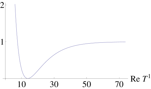
Figure 1: Scalar potential $V_{\rm eff}(T^{1},H_{1})/V_{\infty}$ on the ${\rm Im}\,T^{1}=H_{1}=0$ hypersurface

Before analyzing the inflation dynamics, we should recall the fact that the flatness of the potential in the large ${\rm Re}\,T^{1}$ region is guaranteed by the assumption (11). The most general form of norm function (1) satisfying the condition (11) is found as

$${\cal N}(M) = {\cal P}(M)\,M^{1}+\cdots,$$ (14)

where

$${\cal P}(M) = \sum_{J^{\prime},K^{\prime}\neq 1}^{n_{V}^{\prime}}C_{1,J^{\prime},K^{\prime}}M^{J^{\prime}}M^{K^{\prime}},$$ (15)

is a quadratic polynomial of fields $M^{I^{\prime}\neq 1}$ in $Z_{2}$-odd vector multiplets ${\bm{V}}^{I^{\prime}\neq 1}$ other than ${\bm{V}}^{I^{\prime}=1}$, and the ellipsis stands for terms including fields $M^{I^{\prime\prime}}$ in $Z_{2}$-even vector multiplets ${\bm{V}}^{I^{\prime\prime}}=\{V^{I^{\prime\prime}},\Sigma^{I^{\prime\prime}}\}$ with $I^{\prime\prime}=n_{V}^{\prime}+1,n_{V}^{\prime}+2,\ldots,n_{V}$ whose components $\Sigma^{I^{\prime\prime}}$ are $Z_{2}$-odd chiral multiplets which do not carry any moduli. The coefficient ${\cal P}_{0}$ of ${\rm Re}\,T^{1}$ in Eq. (11) is given by ${\cal P}_{0}={\cal P}({\rm Re}\,T)\Big{|}_{0}$, which is a field independent constant by definition (15).

Therefore, we find that the interesting flat region is realized in a moduli stabilization potential generated by a simple superpotential (2) as a consequence of the peculiar form of norm function (14) in 5D supergravity. Note especially that, the condition (14) cannot be satisfied for $n_{V}^{\prime}=1$, i.e., the single modulus case where only the radion exists, because the norm function ${\cal N}(M)$ is a cubic polynomial. For $n_{V}^{\prime}=2$, the quadratic polynomial ${\cal P}(M)$ is uniquely determined as

$${\cal P}(M) = C_{1,2,2}\,(M^{2})^{2}.$$ (16)

Finally we remark that, although the norm function coefficients $C_{I,J,K}$ are free parameters in 5D supergravity, these are closely related to the structure of the internal manifold, if it is the 5D effective theory of a more fundamental theory defined in more than five dimensional spacetime with extra dimensions compactified on some manifold. In such a situation, the cosmological (as well as phenomenological) features of 5D supergravity are governed by the internal manifold behind it.

3.2 The inflation dynamics

Based on the previous arguments, we identify one of the moduli fields, the real part of the lightest modulus, ${\rm Re}\,T^{1}$, as the inflaton field. Although the inflation mechanism proposed in this paper is applicable to any number $n_{V}^{\prime}\geq 2$ of $Z_{2}$-odd vector multiplets ${\bm{V}}^{I^{\prime}}$, in the following, we choose the minimal number $n_{V}^{\prime}=2$ just for simplicity and concreteness. Then the norm function (14) is uniquely determined by the quadratic monomial (16), where we set $C_{1,2,2}=1$ without loss of generality which determines the normalization of the field $M^{2}$.

By assuming that oscillations of the other light fields ${\rm Im}\,T^{1}$, ${\rm Re}\,H_{1}$ and ${\rm Im}\,H_{1}$ than ${\rm Re}\,T^{1}$ around their expectation values $\langle{\rm Im}\,T^{1}\rangle=\langle{\rm Re}\,H_{1}\rangle=\langle{\rm Im}\,H_{1}\rangle=0$ are negligible during and after the inflation (which will be confirmed in Sec. 4.2), we solve the equation of motion for the single field $\sigma\equiv{\rm Re}\,T^{1}$,

$$\ddot{\sigma}+3H\dot{\sigma}+\Gamma^{\sigma}_{\ \sigma\sigma}\dot{\sigma}^{2}+g^{\sigma\sigma}\frac{\partial V_{\rm eff}}{\partial\sigma} = 0,$$ (17)

where the dot denotes the derivative $\frac{d}{dt}$ with respect to a cosmic time $t$, $V_{\rm eff}$ is the effective potential (9), $g_{\sigma\sigma}=2(K_{\rm eff})_{I^{\prime}=1,J^{\prime}=1}$, $g^{\sigma\sigma}=g_{\sigma\sigma}^{-1}$ and $\Gamma^{\sigma}_{\ \sigma\sigma}$ is the Christoffel symbol constructed by the metric $g_{\sigma\sigma}$, all on the ${\rm Im}\,T^{1}={\rm Re}\,H_{1}={\rm Im}\,H_{1}=0$ hypersurface of the field space. The Hubble parameter $H$ is given as $H^{2}=\left(\frac{\dot{a}}{a}\right)^{2}=\frac{1}{6}g_{\sigma\sigma}\dot{\sigma}^{2}+\frac{V_{\rm eff}}{3}$ where $a$ is the scale factor of 4D spacetime, in which the 4D effective theory of 5D supergravity is defined.

Eq. (17) is rewritten as

$$\sigma^{\prime\prime} = -\left(1-\frac{g_{\sigma\sigma}(\sigma^{\prime})^{2}}{6}\right)\left(3\sigma^{\prime}+6\sigma^{2}\frac{V_{\rm eff}^{\prime}}{V_{\rm eff}}\right)+\frac{(\sigma^{\prime})^{2}}{\sigma},$$ (18)

where the prime denotes the derivative $\frac{d}{dN}=H^{-1}\frac{d}{dt}$ with respect to the number $N\equiv\ln a(t)$ of e-foldings, and we have used $\Gamma^{\sigma}_{\ \sigma\sigma}=-1/\sigma$.

In the following analysis, the numerical values of parameters in the Planck scale unit $M_{\rm Pl}=1$ are chosen as

$$c_{2}^{(2)} = 1/20,\qquad J_{L}^{(2)}/J_{0}^{(2)}\ =\ -9,\qquad J_{0}^{(2)}\ =\ 10^{-1},$$ (19)

for the heavy fields $T^{2}$ and $H^{2}$ as well as those (13) for the light fields $T^{1}$ and $H^{1}$. With these parameters, the vacuum expectation values of fields are given by Eq. (6), and their numerical values are found as

$$\langle T^{1}\rangle\ \simeq\ 13.6,\qquad\langle T^{2}\rangle\ \simeq\ 43.9,\qquad\langle H_{1}\rangle\ =\ \langle H_{2}\rangle\ =\ 0,$$

that determine

$${\cal P}_{0} = {\cal P}({\rm Re}\,T)\Big{|}_{0}\ =\ \langle{\rm Re}\,T^{2}\rangle^{2}.$$

At this supersymmetric Minkowski minimum, the supersymmetric mass squares (7) of light ($I^{\prime}=1$, $i=1$) and heavy ($I^{\prime}=2$, $i=2$) fields are estimated respectively as

$$m^{2}_{I^{\prime}=1,i=1} \simeq \left(4.9\times 10^{12}\ {\rm GeV}\right)^{2},\qquad m^{2}_{I^{\prime}=2,i=2}\ \simeq\ \left(6.9\times 10^{15}\ {\rm GeV}\right)^{2},$$

while the inflation scale in our model is characterized by the Hubble scale

$$H_{\rm inf} \equiv \left(V_{\infty}/3M_{\rm Pl}^{2}\right)^{1/2}\ \simeq\ 1.0\times 10^{12}\ {\rm GeV},$$ (20)

with $V_{\infty}$ given in Eq. (12), for $M_{\rm Pl}=2.4\times 10^{18}$ GeV. Because all of these scales $m_{I^{\prime}=1,i=1}$, $m_{I^{\prime}=2,i=2}$ and $H_{\rm inf}$ are below the compactification scale

$$M_{C} \equiv \frac{\pi}{L}\ \simeq\ \frac{\pi M_{\rm Pl}}{\langle{\cal N}({\rm Re}\,T)\rangle^{1/2}}\ \simeq\ 4.7\times 10^{16}\ {\rm GeV},$$

we find the parameters chosen here ensure the validity of 4D effective-theory description during and after the inflation. It is also confirmed that the heavy fields $T^{2}$ and $H_{2}$ are decoupled from the inflation dynamics due to $m_{I^{\prime}=1,i=1}\sim H_{\rm inf}\ll m_{I^{\prime}=2,i=2}$, and their oscillations can be neglected.

Now we consider a possibility of slow roll inflation starting from a large value of inflaton field $\sigma$ in the flat region of the potential down to its VEV (6) at the minimum. To estimate the observed quantities, we define the generalized slow roll parameters for the scalars having non-canonical kinetic term [15],

$$\epsilon \equiv\frac{M_{Pl}^{2}}{2}\frac{\partial_{\sigma}V_{\rm eff}g^{\sigma\sigma}\partial_{\sigma}V_{\rm eff}}{V_{\rm eff}^{2}}\sim(2c_{1}^{(1)}\sigma)^{2}\left(\frac{J_{L}^{(1)}}{J_{0}^{(1)}}e^{-c_{1}^{(1)}\sigma}\right)^{2},$$

$$\eta \equiv\frac{\nabla^{\sigma}\nabla_{\sigma}V_{\rm eff}}{V_{\rm eff}}=\frac{g^{\sigma\sigma}\partial_{\sigma}^{2}V_{\rm eff}-g^{\sigma\sigma}\Gamma^{\sigma}_{\sigma\sigma}\partial_{\sigma}V_{\rm eff}}{V_{\rm eff}}\sim-(2c_{1}^{(1)}\sigma)^{2}\frac{J_{L}^{(1)}}{J_{0}^{(1)}}e^{-c_{1}^{(1)}\sigma},$$ (21)

where $\nabla_{\sigma}$ is the covariant derivative for the field $\sigma$. The observables such as the power spectrum of scalar curvature perturbation, its spectral index and the tensor-to-scalar ratio are written in terms of these slow-roll parameters as

$$P_{\xi}(k) =\frac{1}{24\pi^{2}}\frac{V}{\epsilon M_{\rm Pl}^{4}},$$

$$n_{s} =1+\frac{d\,{\rm ln}P_{\xi}(k)}{d\,{\rm ln}\,k}\simeq 1-6\,\epsilon+2\,\eta,$$

$$r =16\,\epsilon,$$ (22)

We numerically solve Eq. (18) with the initial conditions $\sigma=117$ and $\sigma^{\prime}=0$ at $N=0$. Fig. 2 shows the evolution of $\sigma$ as a function of $N$. In this figure, we find the inflation ends at about $N_{\rm end}\simeq 70.7$ where the slow-roll condition is violated (max $\{\epsilon,\eta\}\,=\,1$) and then the oscillation of inflaton starts.

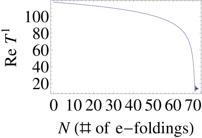
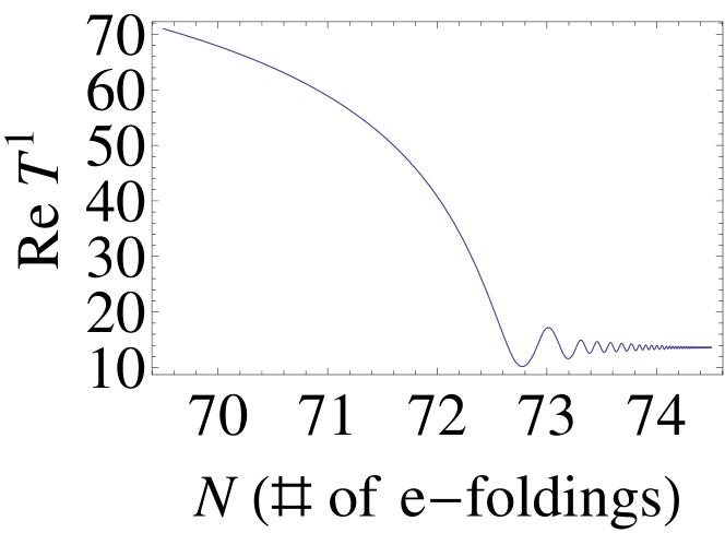
Figure 2: The behavior of inflaton field $\sigma={\rm Re}\,T^{1}$ as a function of the e-folding number $N$.

First, we denote the field value $\sigma=\sigma_{\ast}$ corresponding to the pivot scale $k_{0}=0.05$ [Mpc^-1] (at which the horizon exits) and the scalar potential $V_{\ast}^{1/4}\equiv V^{1/4}(\sigma_{\ast})$ at the pivot scale and $V_{\rm end}^{1/4}\equiv V^{1/4}(\sigma_{\rm end})$ at the end of inflation. In terms of them, the e-folding number after the pivot scale is given by [16],

$$N_{\rm e} \equiv N_{\rm end}-N_{\ast}\simeq\,62+\ln\frac{V_{\ast}^{1/4}}{10^{16}\ {\rm GeV}}+\ln\frac{V_{\ast}^{1/4}}{V_{\rm end}^{1/4}}-\frac{1}{3}\ln\frac{V_{\rm end}^{1/4}}{\rho_{R}^{1/4}}\ \simeq\ 56,$$ (23)

where $V_{\ast}^{1/4}\simeq V_{\rm end}^{1/4}\simeq 2\times 10^{15}$ GeV and $\rho_{R}$ is the energy density by which the universe is thermalized with the reheating temperature $T_{R}\simeq 1.05\times 10^{9}$ GeV whose numerical value will be determined later in Sec. 3.3. Note that the energy of inflaton is assumed, in Eq. (23), to be instantaneously converted into radiation. On the other hand, the same number $N_{\rm e}$ is estimated based on a slow-roll approximation,

$$N_{\rm e}\ =\ -\int_{t_{\rm end}}^{t_{\ast}}d\tilde{t}\,H(\tilde{t})\ \simeq\ \frac{1}{M_{\rm Pl}^{2}}\int_{\sigma_{\rm end}}^{\sigma_{\ast}}d\sigma\frac{V_{\rm eff}}{g^{\sigma\sigma}V^{\prime}_{\rm eff}},$$ (24)

and then we find the numerical value

$$\sigma_{\ast} \simeq 114,$$ (25)

is determined by equaling the Eq. (23) and Eq. (24).

Second, we check whether the WMAP and Planck normalization on the power spectrum of scalar curvature perturbation, $P_{\xi}(k_{0})=2.196_{-0.060}^{+0.051}\times 10^{-9}$  [1], can be realized or not. The slow-roll parameters $\epsilon$ and $\eta$ are obtained at the pivot scale $k_{0}$ by using the numerical value (25),

$$\epsilon \sim(2c_{1}^{(1)}\sigma)^{2}\left(\frac{J_{L}^{(1)}}{J_{0}^{(1)}}e^{-c_{1}^{(1)}\sigma}\right)^{2}\Bigl{|}_{\sigma=\sigma_{\ast}}\simeq{\cal O}(10^{-6}),$$

$$\eta \sim-(2c_{1}^{(1)}\sigma)^{2}\frac{J_{L}^{(1)}}{J_{0}^{(1)}}e^{-c_{1}^{(1)}\sigma}\Bigl{|}_{\sigma=\sigma_{\ast}}\simeq{\cal O}(-0.02),$$ (26)

which yield $P_{\xi}(k_{0})\sim 2\times 10^{-9}$ of the correct order of the observed value. Inversely speaking, the parameters $J_{0}^{(1)}$ and $J_{L}^{(1)}$ are determined in Eq. (13) in such a way that the resultant $P_{\xi}(k_{0})$ resides in the observed region. Also, the spectral index of the scalar curvature perturbation, $n_{s}\,=0.9603\pm 0.0073$  [1], at the pivot scale is observed by the WMAP and Planck collaborations. In our model, we can realize the correct value of the spectral index, $n_{s}\,\simeq\,0.96$ by using Eq. (22) and Eq. (26). It implies that the $\eta$ problem is avoided by the exponential factor and the large value of the inflaton field, because the shift symmetry of $\sigma$ is violated by its own superpotential (8).

We summarize the results of inflation dynamics in Figs. 3 and 4. From these figures drawn with the sample values of parameters (13) and (19), we extract the numerical values of observables as

$$N_{e}=55.6\;\text{e-folds},\qquad P_{\xi}=2.23\times 10^{-9},\qquad n_{s}=0.959,\qquad r=1.6\times 10^{-5}.$$ (27)

So the simple model analyzed so far with Re $T^{1}$ playing the role of inflation is consistent with the WMAP and Planck data [1]. Note that this inflation mechanism is categorized as the small-field model of inflation due to the tiny slow-roll parameter $\epsilon$ and the field variable of the inflaton spends

$$\Delta\hat{\sigma}\equiv\hat{\sigma}_{\ast}-\hat{\sigma}_{\rm end}\simeq 0.77M_{\rm Pl},\;\;\;\hat{\sigma}=\frac{1}{2}{\rm log}\,\sigma,$$ (28)

where we canonically normalize the field $\sigma={\rm Re}\,T^{1}$. This small-field inflation leads to the small tensor-to-scalar ratio as can be seen in Eq. (27). Although the results here are completely consistent with WMAP and the current Planck data, the tiny tensor-to-scalar ratio $r\sim 10^{-5}$ in Eq. (27) contradicts with the most recent data from the BICPE2 collaborations [2]. We discuss how to realize a successful large-field inflation in Sec. 4, which is one of the few candidates to generate a sizable tensor-to-scalar ratio within the framework of single-field slow-roll inflation.

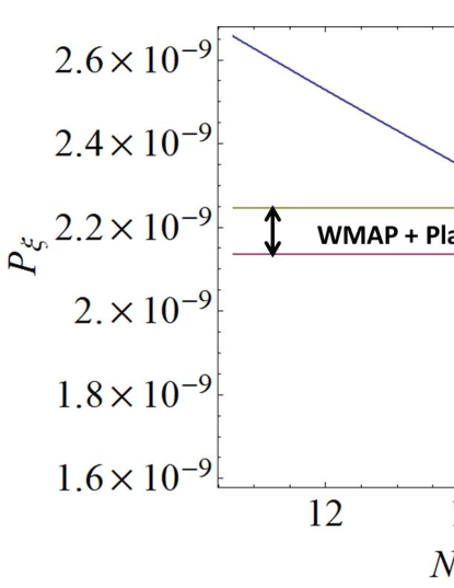
Figure 3: The power spectrum of scalar curvature perturbation between 60 and 50 e-foldings before the end of inflation.

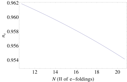
Figure 4: The spectral index of scalar curvature perturbation between 60 and 50 e-foldings before the end of inflation.

3.3 Reheating temperature

Before analyzing the large-field inflation, we comment on the process to reheat the universe. After the inflation, the energy of the inflaton is reduced via inflaton decay into particles in the supersymmetric standard model, although it depends on the concrete model. Here we roughly estimate the reheating temperature via the decay from the inflaton into gauge boson pairs due to the dimensional counting.

If the particles in the supersymmetric standard model have the $U(1)_{I^{\prime}=1}$ charge for the vector multiplet $V^{I^{\prime}=1}$ carrying inflaton, there are terms like $Z_{Q,\bar{Q}}({\rm Re}\,T)|Q|^{2}$ in the Kähler potential with $Q$ being the matter chiral multiplet originated from the hypermultiplet ${\bm{H}}_{\alpha}$ and $Z_{Q,\bar{Q}}({\rm Re}\,T)$ is the Kähler metric of $Q$ given by Eq. (4) where $c_{I^{\prime}}^{(i)}$ is replaced by the $U(1)_{I^{\prime}}$ charge of $Q$. Although these couplings may enhance the inflaton decay width into $Q$, we will not consider them in this paper for simplicity just assuming the vanishing $U(1)_{I^{\prime}=1}$ charges for matter fields. The couplings between moduli and gauge fields are conducted by the gauge kinetic function $f_{a}(T)$, where $a=1,2,3$ represents the gauge groups in the minimal supersymmetric standard model (MSSM), $U(1)_{Y}$, $SU(2)_{L}$, $SU(3)_{c}$ respectively. The relevant terms in the Lagrangian are

$${\cal L} \supset-\cfrac{1}{4}{\rm Re}\,f_{a}F^{a}_{\mu\nu}F^{a\mu\nu}$$

$$=-\cfrac{1}{4}\langle{\rm Re}\,f_{a}\rangle F^{a}_{\mu\nu}F^{a\mu\nu}-\cfrac{1}{4}\left\langle\frac{\partial\,{\rm Re}\,f_{a}}{\partial\hat{\sigma}}\right\rangle\delta\hat{\sigma}F^{a}_{\mu\nu}F^{a\mu\nu},$$ (29)

where $f_{a}=\sum_{I^{\prime}=1}^{2}\xi_{a}^{I^{\prime}}T^{I^{\prime}}$ and $\xi_{a}^{I^{\prime}}\equiv C_{I^{{}^{\prime}},\,J^{{}^{\prime\prime}}=a,\,K^{{}^{\prime\prime}}=a}$. Then the total decay width of the inflaton $\hat{\sigma}$ is approximated as

$$\Gamma\,\simeq\,\sum_{a=1}^{3}\Gamma(\hat{\sigma}\rightarrow g^{(a)}+g^{(a)}) =\sum_{a=1}^{3}\cfrac{N_{G}^{a}}{128\pi}\left\langle\cfrac{\xi_{a}^{1}}{\sqrt{(K_{\rm eff})_{T^{1}T^{1}}}{\rm Re}\,f_{a}}\right\rangle^{2}\cfrac{m_{\hat{\sigma}}^{3}}{M_{Pl}^{2}},$$

$$\simeq\,2.32\,{\rm GeV},$$ (30)

where $\sum_{a=1}^{3}\,N_{G}^{a}\,=\,12$ is the number of the gauge boson in the MSSM and $\hat{\sigma}$ is the canonically normalized inflaton field (28). We choose the $\xi_{1}^{1}=\xi_{2}^{1}=\xi_{3}^{1}=0.27$, otherwise zero to realize the gauge coupling unification at the grand unification scale ($\simeq\,2.0\times 10^{16}{\rm GeV}$),

$$\text{Re}\,f_{a}(\langle T\rangle)=\left(\frac{1}{g_{a}}\right)^{2}\simeq\,3.73.$$ (31)

Then the reheating temperature is roughly estimated by equaling the expansion rate of the universe and the total decay width,

$$\Gamma \simeq\,H(T_{R}),$$

$$\Leftrightarrow T_{R} =\left(\cfrac{\pi^{2}g_{\ast}}{90}\right)^{-1/4}\sqrt{\Gamma\,M_{\rm Pl}}\simeq 1.05\times 10^{9}\,{\rm GeV},$$ (32)

where we use $g_{\ast}=915/4$ which is the effective degrees of freedom of the radiation at the reheating in the MSSM. We restrict ourselves to the standard situation that the coherent oscillation of inflaton field dominates the energy density of the universe after the inflation. The inflaton releases the entropy and reheats the universe when it decay. It is then assumed that the other field does not dominate the energy density of the universe which is verified in Sec. 4.2.

Finally in this section, we mention about the one-loop correction to the moduli Kähler potential. The modified Kähler potential in the large volume limit is found as [17],

$$K=-\ln\,{\cal N}+{\cal O}\left(\frac{1}{32\pi^{2}{\cal N}}\right)+\cdots,$$ (33)

where the leading contribution will depend on the number of the charged fields under the $Z_{2}$-odd vector multiplets $V^{I^{\prime}}$. Even if there are such contributions in the scalar potential, our estimation in the previous section is not changed due to the supersymmetry condition (6) at the vacuum. Since Re $T^{1}$ rolls the potential from the large field value, one-loop effect does not affect the inflation mechanism, which is also confirmed by the numerical analysis.

4 A simple model for the large-field inflation

In this section, we discuss how to realize the large-field inflation that would explain the WMAP, Planck [1] and BICEP2 data [2], although there is a possible tension between these collaborations.

Unlike the previous section, we consider two light pair of modulus and stabilizer fields, e.g. $T^{I^{\prime}=1,2}$ and $H_{i=1,2}$ which are decoupled from the other heavy pairs $T^{I^{\prime}\neq 1,2}$ and $H_{i\neq 1,2}$. This scenario can be realized when $c_{I^{\prime}=1,2}^{(i\neq 1,2)}=c_{I^{\prime}\neq 1,2}^{(i=1,2)}=0$ in Eq. (3), $\left|c_{I^{\prime}\neq 1,2}^{(i\neq 1,2)}\right|<\left|c_{I^{\prime}=1,2}^{(i=1,2)}\right|$ in Eq. (7), $\left|J_{0}^{i=1,2}\right|<\left|J_{0}^{i\neq 1,2}\right|$ and $\left|J_{L}^{i=1,2}\right|<\left|J_{L}^{i\neq 1,2}\right|$ in Eq. (7). Below the heavier mass scale $m_{I^{\prime}\neq 1,2\,i\neq 1,2}$, the effective Kähler potential and superpotential for the light fields $T^{I^{\prime}=1,2}$ and $H_{i=1,2}$ are given by

$$K_{\rm eff}(T^{1},H_{1},T^{2},H_{2}) = -\ln{\cal N}({\rm Re}\,T)\,\Big{|}_{0}+Z_{1,\bar{1}}({\rm Re}\,T)\,\Big{|}_{0}\,|H_{1}|^{2}+Z_{2,\bar{2}}({\rm Re}\,T)\,\Big{|}_{0}\,|H_{2}|^{2},$$

$$W_{\rm eff}(T^{1},H_{1},T^{2},H_{2}) = \left(J_{0}^{(1)}+e^{-c_{I^{\prime}}^{(1)}T^{I^{\prime}}}J_{L}^{(1)}\right)H_{1}+\left(J_{0}^{(2)}+e^{-c_{I^{\prime}}^{(2)}T^{I^{\prime}}}J_{L}^{(2)}\right)H_{2},$$ (34)

where $f(T^{I^{\prime}},H_{i})\,\Big{|}_{0}\equiv f(T^{I^{\prime}},H_{i})\Big{|}_{\scriptsize\begin{array}[]{ll}T^{I^{\prime}\neq 1,2}=\langle T^{I^{\prime}\neq 1,2}\rangle\\ H_{i\neq 1,2}=\langle H_{i\neq 1,2}\rangle\end{array}}$ for an arbitrary function $f(T^{I^{\prime}},H_{i})$, and then

$$Z_{1,\bar{1}}({\rm Re}\,T)\,\Big{|}_{0}=\frac{1-e^{-2c_{I^{\prime}}^{(1)}{\rm Re}\,T^{I^{\prime}}}}{c_{I^{\prime}}^{(1)}{\rm Re}\,T^{I^{\prime}}},\,\,\,\,Z_{2,\bar{2}}({\rm Re}\,T)\,\Big{|}_{0}=\frac{1-e^{-2c_{I^{\prime}}^{(2)}{\rm Re}\,T^{I^{\prime}}}}{c_{I^{\prime}}^{(2)}{\rm Re}\,T^{I^{\prime}}}.$$ (35)

The effective potential for the light fields,

$$V_{\rm eff}(T^{1},H_{1},T^{2},H_{2}) = e^{K_{\rm eff}}\left((K_{\rm eff})^{m,\bar{n}}\,D_{m}W_{\rm eff}\,D_{\bar{n}}\bar{W}_{\rm eff}-3|W_{\rm eff}|^{2}\right),$$ (36)

is obtained by using the effective Kähler potential and superpotential (34), where $m,n=\{I^{\prime},i\}$ with $I^{\prime}=1,2$ and $i=1,2$.

The most general form of part of norm function carrying the two light moduli $T^{1}$ and $T^{2}$ is written as

$${\cal N}({\rm Re}T)\Big{|}_{0} = C_{1,1,1}({\rm Re}T^{1})^{3}+C_{1,1,2}({\rm Re}T^{1})^{2}({\rm Re}T^{2})+C_{1,2,2}({\rm Re}T^{1})({\rm Re}T^{2})^{2}+C_{2,2,2}({\rm Re}T^{2})^{3}$$ (37)

$$+ \cdots,$$

where the ellipsis stands for terms those do not contain the two light moduli. To brighten the outlook for analyzing the above scalar potential (36), we redefine the modulus field as

$$\;\hat{T^{1}}\equiv\frac{c_{1}^{(1)}T^{1}+c_{2}^{(1)}T^{2}}{c},\;\;\;\;\hat{T^{2}}\equiv\frac{c_{1}^{(2)}T^{1}+c_{2}^{(2)}T^{2}}{d}.$$ (38)

where $c$ and $d$ are the $U(1)$ charge of the stabilizer field $H_{1}$ and $H_{2}$ for a linear combination of the $Z_{2}$-odd vector fields $A_{M}^{I^{\prime}}$ in ${\bf V}^{I^{\prime}}$ with $I^{\prime}=1,2$, respectively. In this field base $\hat{T}^{1}$ and $\hat{T}^{2}$, the mixing terms between $\hat{T}^{1}$ and $\hat{T}^{2}$ in the superpotential are canceled and thus each of $\hat{T}^{1}$ and $\hat{T}^{2}$ has the independent superpotential to each other,

$$W_{\rm eff}(\hat{T}^{1},H_{1},\hat{T}^{2},H_{2})\,=\,\left(J_{0}^{(1)}+e^{-c\,\hat{T}^{1}}J_{L}^{(1)}\right)H_{1}+\left(J_{0}^{(2)}+e^{-d\,\hat{T}^{2}}J_{L}^{(2)}\right)H_{2}.$$ (39)

The vacuum expectation values of moduli $\hat{T}^{1},\hat{T}^{2}$ and stabilizer fields $H_{1},H_{2}$ are determined by minimizing the scalar potential (36) in a similar way to those of the small-field inflation (6) as

$$\langle\hat{T}^{1}\rangle = \frac{1}{c}\ln\frac{J_{L}^{(1)}}{J_{0}^{(1)}},\qquad\langle\hat{T}^{2}\rangle\ =\ \frac{1}{d}\ln\frac{J_{L}^{(2)}}{J_{0}^{(2)}},\qquad\langle H_{1}\rangle\ =\ \langle H_{2}\rangle\ =\ 0,$$ (40)

which satisfy $\langle D_{\hat{I}^{\prime}}W\rangle=\langle D_{i}W\rangle=\langle W\rangle=0$ and then $\langle V_{\hat{I}^{\prime}}\rangle=\langle V_{i}\rangle=\langle V\rangle=0$ for $V_{m}=\partial_{m}V$.

When we construct the large-field inflation model in the next subsection, we restrict ourselves to the case that the coefficients $C_{I^{\prime},J^{\prime},K^{\prime}}$ and the charges $c_{I^{\prime}}^{(i)}$ for $I^{\prime},J^{\prime},K^{\prime}=1,2$ and $i=1,2$ are chosen in such a way that the norm function is written as

$${\cal N}({\rm Re}T)\Big{|}_{0}=a({\rm Re}\hat{T}^{1})({\rm Re}\hat{T}^{2}-b\,{\rm Re}\hat{T}^{1})^{2}+\cdots,$$ (41)

in the hatted field base, where $a$ and $b$ are positive real numbers determined by the fixed values of $C_{I^{\prime},J^{\prime},K^{\prime}}$ and $c_{I^{\prime}}^{(i)}$ as, e.g., $a=c_{1}^{(1)}(d)^{2}/c\,(c_{2}^{(2)})^{2},b=c\,c_{1}^{(2)}/d\,c_{1}^{(1)}$ for $c_{2}^{(1)}=C_{1,1,1}=C_{1,1,2}=C_{2,2,2}=0$ and $C_{1,2,2}=1$. The ellipsis in Eq. (41) has same meaning as that in Eq. (37) and is irrelevant in the following arguments. The advantage of the norm function (41) will be explained in Sec. 4.1, and here we notice that it leads to the moduli mixing in the Kähler metric, $K_{\hat{I}^{{}^{\prime}},\bar{\hat{J}}^{{}^{\prime}}}\neq 0$ for $\hat{I}^{{}^{\prime}}\neq\hat{J}^{{}^{\prime}}$. We have to check the positivity of the Hessian matrix with the scalar potential (36). The mass matrix given by the potential (36) is written in a block-diagonal form with two nonvanishing blocks according to the absence mixing terms between the moduli $\hat{T}^{I^{\prime}=1,2}$ and the stabilizer fields $H_{i=1,2}$. Since the following mixing terms are all vanishing at the vacuum,

$$\langle V_{\hat{T}^{1}\bar{\hat{T}}^{2}}\rangle=\langle V_{\hat{T}^{1}\bar{H}_{1}}\rangle=\langle V_{\hat{T}^{1}\bar{H}_{2}}\rangle=\langle V_{\hat{T}^{2}\bar{H}_{1}}\rangle=\langle V_{\hat{T}^{2}\bar{H}_{2}}\rangle=0,$$

$$\langle(K_{\rm eff})^{\hat{T}^{1}\bar{H}_{1}}\rangle=\langle(K_{\rm eff})^{\hat{T}^{1}\bar{H}_{2}}\rangle=\langle(K_{\rm eff})^{\hat{T}^{2}\bar{H}_{1}}\rangle=\langle(K_{\rm eff})^{\hat{T}^{2}\bar{H}_{2}}\rangle=0,$$ (42)

for $V_{mn}=\partial_{n}\partial_{m}V$, there are no mixing between the moduli $\hat{T}^{I^{\prime}}$ and the stabilizer fields $H_{i}$ at the vacuum, that is, the mass (sub-)matrices of the moduli $\hat{T}^{I^{\prime}}$ and the stabilizer fields $H_{i}$ can be analyzed independently.

First, we consider the mass-squared matrix $m_{t}^{2}$ of the real parts of the moduli in the base of canonically normalized field $t^{I^{\prime}}$,

$$t^{I^{\prime}}\,=\,\sum_{J^{\prime}=1}^{2}\sqrt{2(K_{\hat{T}})_{I^{\prime}}}U_{I^{\prime},J^{\prime}}{\rm Re}\,\hat{T}^{J^{\prime}},$$ (43)

for $I^{\prime}=1,2$, which is estimated as

$$m_{t}^{2}=\begin{pmatrix}\sqrt{\frac{1}{(K_{\hat{T}})_{1}}}&0\\ 0&\sqrt{\frac{1}{(K_{\hat{T}})_{2}}}\end{pmatrix}U\begin{pmatrix}V_{\hat{T}^{1}\bar{\hat{T}}^{1}}&0\\ 0&V_{\hat{T}^{2}\bar{\hat{T}}^{2}}\end{pmatrix}U^{-1}\begin{pmatrix}\sqrt{\frac{1}{(K_{\hat{T}})_{1}}}&0\\ 0&\sqrt{\frac{1}{(K_{\hat{T}})_{2}}}\end{pmatrix},$$ (44)

where $V_{\hat{T}^{I^{\prime}}\bar{\hat{T}}^{J^{\prime}}}=\langle e^{K_{\rm eff}}(K_{\rm eff})^{H_{i}\bar{H}_{j}}W_{\hat{T}^{I^{\prime}}H_{i}}\overline{W_{\hat{T}^{J^{\prime}}H_{j}}}\rangle$, and $(K_{\hat{T}})_{1}$, $(K_{\hat{T}})_{2}$ and $U$ are the eigenvalues and diagonalizing matrix of the moduli Kähler metric, respectively. (Explicit form of them are shown in Appendix A.) By contrast, the mass-squared matrix of the imaginary part, ${\rm Im}\,\hat{T}^{1}$ and ${\rm Im}\,\hat{T}^{2}$, is already diagonalized because Kähler potential does not contain the imaginary parts of moduli, those are prohibited by the $U(1)$ gauge symmetries. The supersymmetric masses of canonically normalized moduli $\phi^{I^{\prime}}$,

$$\phi^{I^{\prime}}\,=\,\sqrt{2(K_{\rm eff})_{\hat{T}^{I^{\prime}}\bar{\hat{T}}^{I^{\prime}}}}\,{\rm Im}\,\hat{T}^{I^{\prime}},$$ (45)

for $I^{\prime}=1,2$, are also same as those shown in Eq. (7) where the Kähler potential and superpotential are replaced by Eq. (34).

Second, the mass-squared matrix of the stabilizer field is also evaluated in the base of canonically normalized field $h_{i}$,

$$h_{i}\,=\,\sum_{j=1}^{2}\sqrt{2(K_{H})_{i}}\delta_{i,j}H_{j},$$ (46)

for $i=1,2$, that is found as

$$m_{h}^{2}=\begin{pmatrix}\sqrt{\frac{1}{(K_{H})_{1}}}&0\\ 0&\sqrt{\frac{1}{(K_{H})_{2}}}\end{pmatrix}\begin{pmatrix}V_{H_{1}\bar{H}_{1}}&V_{H_{1}\bar{H}_{2}}\\ V_{H_{2}\bar{H}_{1}}&V_{H_{2}\bar{H}_{2}}\end{pmatrix}\begin{pmatrix}\sqrt{\frac{1}{(K_{H})_{1}}}&0\\ 0&\sqrt{\frac{1}{(K_{H})_{2}}}\end{pmatrix},$$ (47)

where $V_{H_{i}\bar{H}_{j}}=\langle e^{K_{\rm eff}}(K_{\rm eff})^{\hat{T}^{I^{\prime}}\bar{\hat{T}}^{J^{\prime}}}W_{\hat{T}^{I^{\prime}}H_{i}}\overline{W_{\hat{T}^{J^{\prime}}H_{j}}}\rangle$, and $(K_{H})_{1}=\langle(K_{\rm eff})_{H_{1}\bar{H}_{1}}\rangle$, $(K_{H})_{2}=\langle(K_{\rm eff})_{H_{2}\bar{H}_{2}}\rangle$ are the eigenvalues of the Kähler metric of the stabilizer fields, respectively.

From the mass-squared matrices (44) and (47), the supersymmetric masses of the canonically normalized stabilizer fields $h_{i}$ and the moduli $t^{I^{\prime}}$ in the limit of $\langle W_{\hat{T}^{1}H_{1}}\rangle\ll\langle W_{\hat{T}^{2}H_{2}}\rangle$ are estimated as,

$$m_{t^{1}}^{2}\simeq\frac{e^{\langle K_{\rm eff}\rangle}\langle(K_{\rm eff})^{H_{1}\bar{H}_{1}}\rangle\langle W_{\hat{T}^{1}H_{1}}\rangle^{2}}{\langle(K_{\rm eff})_{\hat{T}_{1}\bar{\hat{T}}_{1}}\rangle},\qquad m_{t^{2}}^{2}\simeq e^{\langle K_{\rm eff}\rangle}\langle(K_{\rm eff})^{H_{2}H_{2}}\rangle\langle(K_{\rm eff})^{\hat{T}^{2}\bar{\hat{T}}^{2}}\rangle\langle W_{\hat{T}^{2}H_{2}}\rangle^{2},$$

$$m_{{\rm Re}\,h_{1}}^{2}=m_{{\rm Im}\,h_{1}}^{2}\simeq\frac{e^{\langle K_{\rm eff}\rangle}\langle(K_{\rm eff})^{\hat{T}^{1}\bar{\hat{T}}^{1}}\rangle\langle W_{\hat{T}^{1}H_{1}}\rangle^{2}}{\langle(K_{\rm eff})_{H_{1}\bar{H}_{1}}\rangle},$$

$$m_{{\rm Re}\,h_{2}}^{2}=m_{{\rm Im}\,h_{2}}^{2}\simeq\frac{e^{\langle K_{\rm eff}\rangle}\langle(K_{\rm eff})^{\hat{T}^{2}\bar{\hat{T}}^{2}}\rangle\langle W_{\hat{T}^{2}H_{2}}\rangle^{2}}{\langle(K_{\rm eff})_{H_{2}\bar{H}_{2}}\rangle}.$$ (48)

These expressions show that the squared masses of moduli and stabilizers are all positive at the vacuum if there is a hierarchy $\langle W_{\hat{T}^{1}H_{1}}\rangle\ll\langle W_{\hat{T}^{2}H_{2}}\rangle$ as mentioned in Sec. 2, that confirms the stability of the vacuum (40).

Because the two pair $(\hat{T}^{1},H_{1})$ and $(\hat{T}^{2},H_{2})$ of modulus and stabilizer have totally independent vacuum expectation values to each other as shown in Eq. (40), we can further consider the situation that the first pair ($\hat{T}^{1},H_{1}$) is lighter than the second pair ($\hat{T}^{2},H_{2}$) by assuming $\left|J_{0}^{1}\right|<\left|J_{0}^{2}\right|$ and $\left|J_{L}^{1}\right|<\left|J_{L}^{2}\right|$. In this case, the second pair can also be integrated out, and the effective potential for the first pair is given by

$$V_{\rm eff}(\hat{T}^{1},H_{1}) = e^{K_{\rm eff}}\left((K_{\rm eff})^{m,\bar{n}}\,D_{m}W_{\rm eff}\,D_{\bar{n}}\bar{W}_{\rm eff}-3|W_{\rm eff}|^{2}\right),$$ (49)

where $m,n=\{\hat{I}^{\prime},i\}$ with $\hat{I}^{\prime}=1$ and $i=1$ and the effective Kähler potential $K_{\rm eff}$ and superpotential $W_{\rm eff}$ are obtained as

$$K_{\rm eff}(\hat{T}^{1},H_{1}) = -\ln{\cal N}({\rm Re}\,\hat{T})\,\Big{|}_{0}+Z_{1,\bar{1}}({\rm Re}\,\hat{T})\,\Big{|}_{0}\,|H_{1}|^{2},$$

$$W_{\rm eff}(\hat{T}^{1},H_{1}) = \left(J_{0}^{(1)}+e^{-c\,\hat{T}^{1}}J_{L}^{(1)}\right)H_{1}.$$ (50)

Here we adopt the notation $f(T^{I^{\prime}},H_{i})\,\Big{|}_{0}\equiv f(T^{I^{\prime}},H_{i})\Big{|}_{\scriptsize\begin{array}[]{lll}T^{I^{\prime}\neq 1,2}=\langle T^{I^{\prime}\neq 1,2}\rangle\\ \hat{T}^{I^{\prime}\neq 2}=\langle\hat{T}^{I^{\prime}\neq 2}\rangle\\ H_{i\neq 1}=\langle H_{i\neq 1}\rangle\\ \end{array}}$ for an arbitrary function $f(T^{I^{\prime}},H_{i})$.

4.1 The Inflation potential and dynamics

From the above scalar potential (49), we find the effective potential for the modulus $\hat{T}^{1}$ on the $H_{1}=0$ hypersurface,

$$V_{\rm eff}(\hat{T}^{1},H_{1}=0) = e^{K_{\rm eff}}(K_{\rm eff})^{i=1,\bar{i}=\bar{1}}\left|(W_{\rm eff})_{i=1}\right|^{2}\,\Big{|}_{H_{1}=0}$$ (51)

$$= \Lambda^{4}(1-\lambda\,\text{cos}(c\,\tau)),$$

where

$$\Lambda^{4} \equiv \frac{c}{(\langle{\rm Re}\,\hat{T}^{2}\rangle-b\,\sigma)^{2}}\frac{J_{01}^{2}+J_{L1}^{2}e^{-2c\,\sigma}}{1-e^{-2c\,\sigma}},$$

$$\lambda \equiv 2\cfrac{J_{01}J_{L1}e^{-c\,\sigma}}{J_{01}^{2}+J_{L1}^{2}e^{-2c\,\sigma}},$$ (52)

we adopted the norm function (41) with $a=1$ and $\hat{T}^{1}=\sigma+i\tau$. Fig. 5 shows the scalar potential on the $(\sigma,\tau)$-plane, where the parameters are chosen as

$$c=1/30,\qquad J_{L}^{(1)}\,=\,-4.4\times 10^{-3},\qquad J_{0}^{(1)}\,=\,4.25\times 10^{-3},\qquad b=15,$$ (53)

in the Planck unit $M_{{\rm Pl}}=1$. The imaginary direction $\tau$ has a periodic property as can be seen in Eq. (51) and the real direction $\sigma$ will be stabilized at the minimum shown in Fig. 6 in which the behaviors of potential on the hypersurfaces $\tau=10$ (dot dashed line), $\tau=5$ (dashed line) and $\tau=0$ (thick line) are drawn. As we can see from Fig. 6, the negative region of $\sigma<0$ is not allowed, because the $\Lambda$ in Eq. (51) diverges in the limit of $\sigma\rightarrow 0$, while the overshooting to a large-field region, $\sigma>$ $\langle{\rm Re}\,\hat{T}^{2}\rangle/b$, is also prohibited by the structure of the norm function (41). Since Re $\hat{T}^{2}$ is already stabilized by its own minimum (40), we find

$$\lim_{{\rm Re}\,\hat{T}^{1}\to\langle{\rm Re}\,\hat{T}^{2}\rangle/b}\left|V_{\rm eff}(\hat{T}^{1},H_{1}=0)\right|=\infty.$$ (54)

From these properties of the potential (51), we expect that the so-called natural inflation [18] would occur by identifying $\tau={\rm Im}\,\hat{T}^{1}$ as the inflaton field. During the inflation, the real part $\sigma$ will take a different field value from the one at the true minimum (40) and after the inflation, it rolls down to the minimum and oscillates around the vacuum.

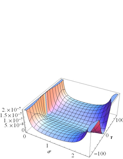
Figure 5: The scalar potential (51) on the $(\sigma,\tau)$-plane.

Figure 6: The scalar potential (51) on the hypersurfaces $\tau=10$ (dotdashed line), $\tau=5$ (dashed line) and $\tau=0$ (thick line).

To confirm the above statements, we solve the equations of motion for two fields $\sigma$ and $\tau$ under the assumption that the oscillations of the stabilizer fields, Re $H_{1}$ and Im $H_{1}$, around their vacuum expectation values $\langle{\rm Re}\,H_{1}\rangle=\langle{\rm Im}\,H_{1}\rangle=0$ are negligible during and after the inflation (which will be confirmed in Sec. 4.2). The equations of motion for these fields are written as

$$\sigma^{{}^{\prime\prime}} =-\left(1-{\cal L}_{\text{kin}}\right)\left(3\sigma^{{}^{\prime}}+6\frac{\sigma^{2}(\langle\hat{T}^{2}\rangle-b\sigma)^{2}}{(\langle\hat{T}^{2}\rangle-b\sigma)^{2}+2b^{2}\sigma^{2}}\frac{\partial_{\sigma}V}{V}\right)+\frac{(\sigma^{{}^{\prime}})^{2}-(\tau^{{}^{\prime}})^{2}}{\sigma(\langle\hat{T}^{2}\rangle-b\sigma)}\left(\frac{(\langle\hat{T}^{2}\rangle-b\sigma)^{3}-2b^{3}\sigma^{3}}{(\langle\hat{T}^{2}\rangle-b\sigma)^{2}+2b^{2}\sigma^{2}}\right),$$

$$\tau^{{}^{\prime\prime}} =-\left(1-{\cal L}_{\text{kin}}\right)\left(3\tau^{{}^{\prime}}+6\frac{\sigma^{2}(\langle\hat{T}^{2}\rangle-b\sigma)^{2}}{(\langle\hat{T}^{2}\rangle-b\sigma)^{2}+2b^{2}\sigma^{2}}\frac{\partial_{\tau}V}{V}\right)+\frac{2\sigma^{{}^{\prime}}\tau^{{}^{\prime}}}{\sigma(\langle\hat{T}^{2}\rangle-b\sigma)}\left(\frac{(\langle\hat{T}^{2}\rangle-b\sigma)^{3}-2b^{3}\sigma^{3}}{(\langle\hat{T}^{2}\rangle-b\sigma)^{2}+2b^{2}\sigma^{2}}\right),$$

$${\cal L}_{\text{kin}} \equiv\frac{(\langle\hat{T}^{2}\rangle-b\sigma)^{2}+2b^{2}\sigma^{2}}{2\sigma^{2}(\langle\hat{T}^{2}\rangle-b\sigma)^{2}}\left((\sigma^{{}^{\prime}})^{2}+(\tau^{{}^{\prime}})^{2}\right),$$ (55)

where the prime denotes the derivative $d/dN$ with respect to the number $N$ of e-foldings as before, and we described the Christoffel symbol for the target space in terms of the metric $g_{\sigma\sigma}=g_{\tau\tau}=\frac{(\langle\hat{T}^{2}\rangle-b\sigma)^{2}+2b^{2}\sigma^{2}}{2\sigma^{2}(\langle\hat{T}^{2}\rangle-b\sigma)^{2}}$.

In the following analysis, the numerical values of parameters in the Planck unit $M_{{\rm Pl}}=1$ are chosen as

$$d\,=\,1/20,\qquad J_{L}^{(2)}/J_{0}^{(2)}\,=\,-9,\qquad J_{0}^{(0)}\,=\,10^{-1},$$ (56)

for the heavier fields $\hat{T}^{2}$ and $H_{2}$ as well as those (53) for the light fields $\hat{T}^{1}$ and $H_{1}$. With these parameters, the vacuum expectation values of fields are given by

$$\langle\hat{T}^{1}\rangle\simeq 1.04,\qquad\langle\hat{T}^{2}\rangle\,=\,43.94,\qquad\langle H_{1}\rangle\,=\,\langle H_{2}\rangle\,=\,0.$$ (57)

For the canonically normalized fields (43), (45) and (46), their vacuum expectation values are

$$\langle t^{1}\rangle\simeq 2.29,\qquad\langle t^{2}\rangle\,\simeq\,1.22,\qquad\langle\phi^{1}\rangle\,=\,\langle\phi^{2}\rangle\,=\,\langle h_{1}\rangle\,=\,\langle h_{2}\rangle\,=\,0.$$ (58)

The supersymmetric masses (7) and (48) of these fields $t^{I^{\prime}}$,$\phi^{I^{\prime}}$ and $h_{i}$ are estimated as

$$(m_{t^{1}})^{2}\simeq(m_{\phi^{1}})^{2}\simeq(m_{{\rm Re}\,h_{1}})^{2}=(m_{{\rm Im}\,h_{1}})^{2}\simeq\left(1.96\times 10^{13}\,{\rm GeV}\right)^{2},$$

$$(m_{t^{2}})^{2}\simeq(m_{{\rm Re}\,h_{2}})^{2}=(m_{{\rm Im}\,h_{2}})^{2}\simeq\left(4.45\times 10^{16}\,{\rm GeV}\right)^{2},$$

$$(m_{\phi^{2}})^{2}\simeq\left(3.5\times 10^{16}\,{\rm GeV}\right)^{2}.$$ (59)

Note that the supersymmetric masses of $\phi^{I^{\prime}}$ are in general different from those of $t^{I^{\prime}}$ due to the different canonical normalization of Re$\,\hat{T}^{I^{\prime}}$ and Im$\,\hat{T}^{I^{\prime}}$ from each other. The Hubble scale is given by

$$H_{\rm inf}\,=\,\left(V_{\rm inf}/3M_{\rm Pl}^{2}\right)^{1/2}\simeq 8.6\times 10^{13}{\rm GeV},$$ (60)

where $V_{\rm inf}\sim\Lambda^{4}$ is estimated by Eq. (51). We check that these masses (59) and Hubble scale (60) are below the compactification scale $M_{C}\simeq\pi M_{\rm Pl}/\langle{\cal N}({\rm Re}\,\hat{T})\rangle^{1/2}\simeq 2.6\times 10^{17}{\rm GeV}$ to ensure the validity of 4D effective-theory description. The pair ($\hat{T}^{2},H_{2}$) is stabilized at $\hat{T}^{1}$- and $H_{1}$-independent minimum and their masses are larger than the inflaton scale, that is, $H_{\rm inf}^{2}\ll(m_{t^{2}}^{2}),\,(m_{\phi^{2}}^{2}),\,(m_{{\rm Re}\,h^{2}}^{2}),\,(m_{{\rm Im}\,h^{2}}^{2})$. Then the heavier pair ($\hat{T}^{2},H_{2}$) is decoupled from the inflation dynamics.

Next we define the slow-roll parameters for the multi-field case [15] to estimate the observable quantities constrained by the cosmological observations,

$$\epsilon =\,\frac{g^{\sigma\sigma}}{2}\left(\frac{\partial_{\sigma}V}{V}\right)^{2}+\frac{g^{\tau\tau}}{2}\left(\frac{\partial_{\tau}V}{V}\right)^{2},$$

$$\eta =\,\text{minimum eigenvalue of}\;\left\{\frac{1}{V}\begin{pmatrix}\nabla^{i}\nabla_{j}V&\nabla^{i}\nabla_{\bar{j}}V\\ \nabla^{\bar{i}}\nabla_{j}V&\nabla^{\bar{i}}\nabla_{\bar{j}}V\end{pmatrix}\right\},$$

$$=\frac{g^{\sigma\sigma}}{2}\left(\frac{\partial_{\sigma}\partial_{\sigma}V}{V}+\frac{\partial_{\tau}\partial_{\tau}V}{V}-\sqrt{\left(\frac{\partial_{\sigma}\partial_{\sigma}V}{V}-\frac{\partial_{\tau}\partial_{\tau}V}{V}-2\Gamma^{\sigma}_{\sigma\sigma}\frac{\partial_{\sigma}V}{V}\right)^{2}+4\left(\frac{\partial_{\sigma}\partial_{\tau}V}{V}-\Gamma^{\sigma}_{\sigma\sigma}\frac{\partial_{\tau}V}{V}\right)^{2}}\right),$$ (61)

where $i,j\,=\,\sigma,\tau$. The observables such as the power spectrum $P_{\xi}(k)$ of scalar curvature perturbation, its spectral index $n_{s}$ and the tensor-to-scalar ratio $r$ are written in terms of these slow-roll parameters,

$$P_{\xi}(k) =\frac{1}{24\pi^{2}}\frac{V}{\epsilon\,M_{Pl}^{4}},$$

$$n_{s} =1+\frac{d\,{\rm ln}P_{\xi}(k)}{d\,{\rm ln}\,k}\simeq 1-6\epsilon+2\eta,$$

$$r =16\,\epsilon.$$ (62)

We numerically solve Eq. (55) with the initial conditions $(\sigma,\tau)=(1,20)$ and $(\sigma^{{}^{\prime}},\tau^{{}^{\prime}})=(0,0)$ at $N=0$ and then Fig. 7 shows the evolution of $\sigma$ and $\tau$ as a function of $N$. The time at the end of inflation corresponds to an about $N_{\rm end}\simeq 81.2$ e-folds, when the slow-roll condition is violated (max $\{\epsilon,\eta\}=1$). Fig. 7 confirms a desired situation that the real part $\sigma$ of the light modulus is fixed to a certain field value different from its vacuum expectation value during the inflation and oscillates around the vacuum after the inflation. Such a dynamics is explained as follows. The mass square of $\sigma$ consists of those from the Hubble-induced and the supersymmetric contributions,

$$\partial_{\sigma}\partial_{\sigma}V \simeq\,3f(\sigma)H_{\rm inf}^{2}+m_{\rm SUSY}^{2},$$ (63)

where $H_{\rm inf}$ is the inflation scale defined by Eq. (60), $m_{\rm SUSY}\sim m_{t^{1}}\sim{\cal O}(10^{13}\,{\rm GeV})$ is the supersymmetric mass term originating from the superpotential (34) and $f(\sigma)$ is a function of $\sigma$ whose numerical value is of ${\cal O}(1)$ during and after the inflation. By virtue of the Hubble-induced contribution in Eq. (63), the real part $\sigma$ is “stabilized” (at a different point from the minimum of potential) with its field value estimated below during the inflation caused by the slowly rolling imaginary part $\tau$ playing a role of inflaton field.

The “stabilized” value of $\sigma$ during the inflation can be estimated analytically from the approximated equation of motion for $\sigma$ under the slow-roll regime, $\sigma^{{}^{\prime}}\ll 1$ and $\tau^{{}^{\prime}}\ll 1$,

$$\sigma^{{}^{\prime}} =-g^{\sigma\sigma}\frac{V_{\sigma}}{V}$$

$$=-g^{\sigma\sigma}\left(\frac{2}{\langle\hat{T}^{2}\rangle/b-\,\sigma}-\frac{2c\,e^{-2c\,\sigma}}{1-e^{-2c\,\sigma}}-c\right)+\frac{V_{\rm vac}(\sigma)}{V},$$ (64)

where $V_{\rm vac}(\sigma)=e^{K_{\rm eff}}(K_{\rm eff})^{H_{1}\bar{H}_{1}}c\left(\left|J_{0}^{(1)}\right|^{2}-\left|J_{L}^{(1)}\right|^{2}e^{-2c\,\sigma}\right)/{\cal N}$ and we dropped the mixing term proportional to $\sigma^{{}^{\prime}}\tau^{{}^{\prime}}$. The field value $\sigma=\sigma_{\rm inf}$ during the inflation is given by equaling the first parenthesis of Eq. (64) to $0$,

$$\frac{2}{\langle\hat{T}^{2}\rangle/b-\,\sigma_{\rm inf}}-\frac{2c\,e^{-2c\,\sigma_{\rm inf}}}{1-e^{-2c\,\sigma_{\rm inf}}}-c\,=\,0,$$

$$\Leftrightarrow \frac{\langle\hat{T}^{2}\rangle}{b}\,=\,\frac{-2+c\,\sigma_{\rm inf}+e^{2c\,\sigma_{\rm inf}}(2+c\,\sigma_{\rm inf})}{c\,(1+e^{2c\,\sigma_{\rm inf}})}.$$ (65)

One of the advantages of the current setup in our model building is that we can choose the value of $\sigma_{\rm inf}$ close to the vacuum expectation value $\langle\sigma\rangle$ at the minimum of potential given by Eq. (40), if we employ the parameters of the heavier modulus $\hat{T}^{2}$ in such a way that the following relation holds,

$$\frac{\langle\hat{T}^{2}\rangle}{b}\,\simeq\,\frac{-2+c\,\langle\sigma\rangle+e^{2c\,\langle\sigma\rangle}(2+c\,\langle\sigma\rangle)}{c\,(1+e^{2c\,\langle\sigma\rangle})},$$ (66)

which is already adopted in the above numerical analysis. Therefore, the inflaton dynamics caused by the light modulus field $\hat{T}^{1}=\sigma+i\tau$ can be dominated by its imaginary part $\tau$, and then it is classified as a single-field inflation which can avoid sizable magnitudes of the isocurvature perturbations possibly caused by the dynamics of the other fields (most likely $\sigma$) than the inflaton. As the inflaton $\tau$ rolls down toward the minimum (40), the real part $\sigma$ also tends to go there, because the value of $V$ approaches $V_{\rm vac}$ shown in Eq. (64). The discussion here is confirmed in Fig. 8, where the black dotted curve is the inflationary trajectory on the ($\tau$, $\sigma$)-plane evaluated under the slow-roll approximation (64) and the red solid curve represents the same trajectory by solving the full equations of motion (55) numerically.

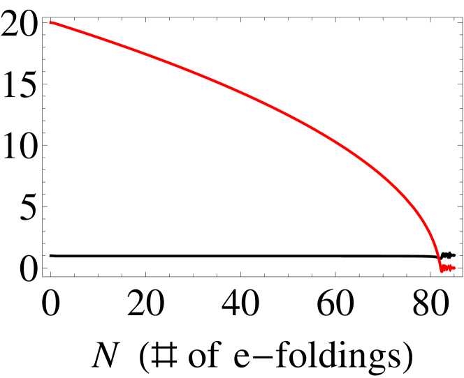
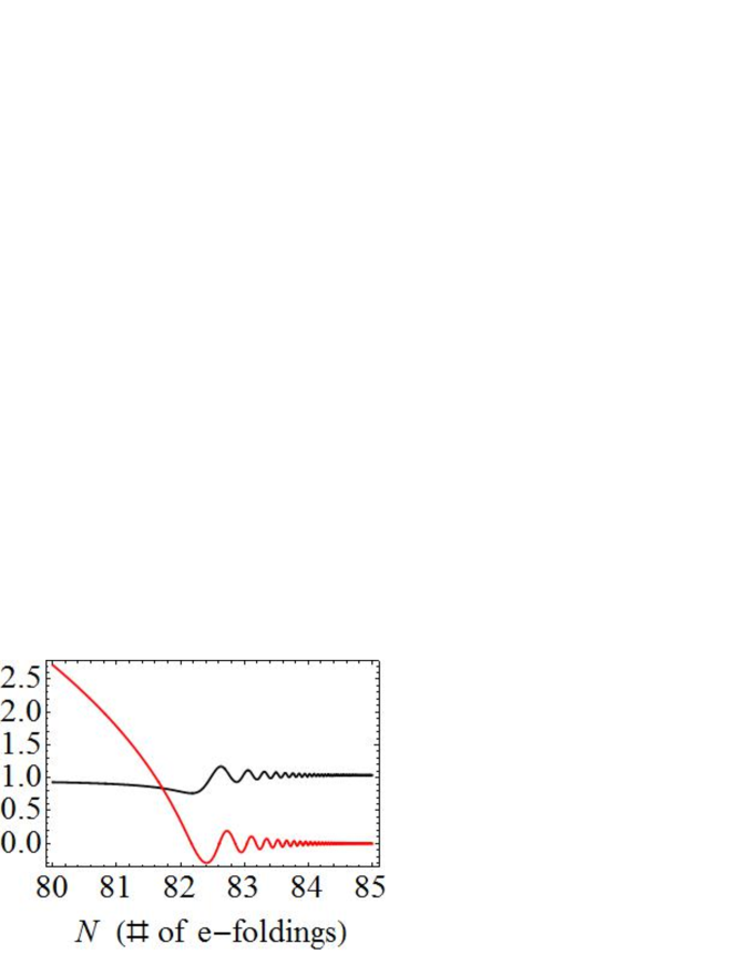
Figure 7: The behavior of the $\sigma={\rm Re}\,\hat{T}^{1}$ (black curves) and $\tau={\rm Im}\,\hat{T}^{1}$ (red curves) as a function of the e-folding number $N$.

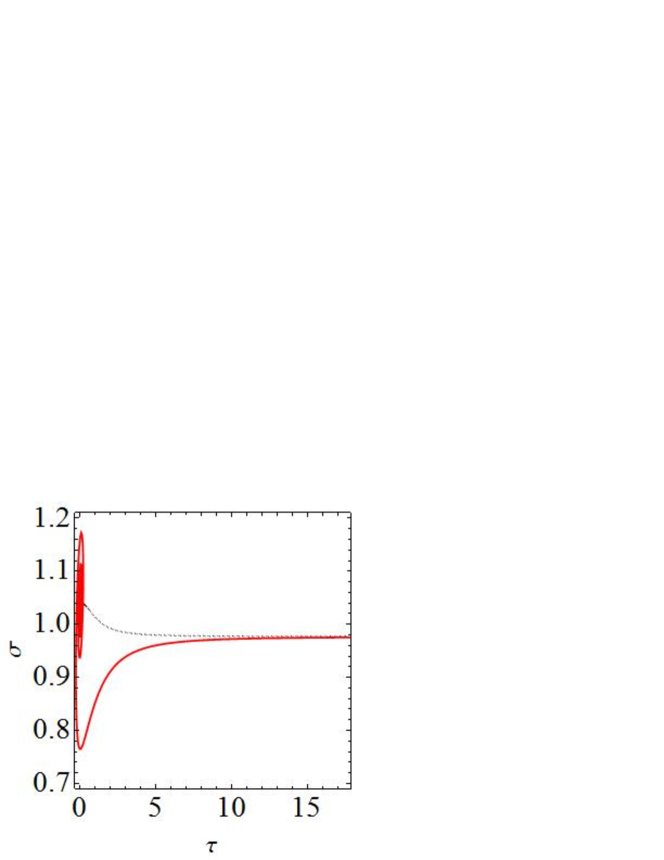
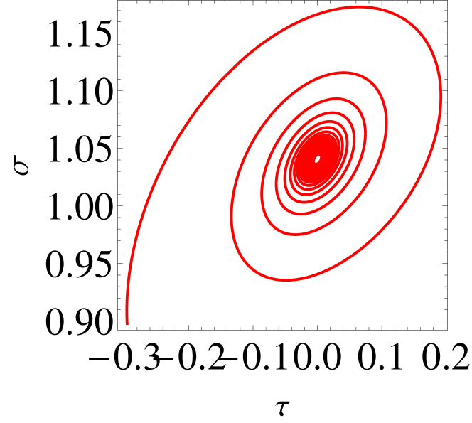
Figure 8: The inflaton trajectory on the ($\tau-\sigma$)-plane. (The black dotted curve is evaluated under the slow-roll approximation (64), while the red solid curve is drawn by solving the full equations of motion (55) numerically.)

From the observational point of view, the above inflationary dynamics can be considered as a single-field inflation if the scalar density perturbation is successfully produced and in this case the inflation mechanism is essentially categorized into the so-called natural inflation [18]. (With our parameter settings, the value of $\lambda$ defined in Eq. (52) is almost equal to $1$ due to $\sigma_{\rm inf}\sim\langle\sigma\rangle$ caused by the parameter choice (53)). Therefore the effective potential for the canonically normalized field $\phi^{1}\equiv k\tau$ is given by

$$V_{\rm eff}=\Lambda^{4}(1-\lambda\,(\hat{c}\,\phi^{1})),$$ (67)

where $\hat{c}\equiv c/k$ and $k\equiv\sqrt{2(K_{\rm eff})_{\hat{T}^{1}\bar{\hat{T}}^{1}}}=\sqrt{\frac{(\langle T^{2}\rangle-b\,\sigma)^{2}+2b^{2}\,\sigma^{2}}{2\sigma^{2}(\langle T^{2}\rangle-b\,\sigma)^{2}}}$ and the slow-roll parameters are explicitly shown in terms of $\phi^{1}$ as

$$\epsilon =\frac{M_{\rm Pl}^{2}}{2}\left(\frac{V^{{}^{\prime}}}{V}\right)^{2}=\frac{(\hat{c}\,M_{\rm Pl})^{2}}{2}\lambda^{2}\frac{1-{\rm cos}^{2}(\hat{c}\,\phi^{1})}{\left(1-\lambda\,{\rm cos}(\hat{c}\,\phi^{1})\right)^{2}},$$

$$\eta =M_{\rm Pl}^{2}\frac{V^{{}^{\prime\prime}}}{V}=(\hat{c}\,M_{\rm Pl})^{2}\lambda\frac{{\rm cos}(\hat{c}\,\phi^{1})}{1-\lambda\,{\rm cos}(\hat{c}\,\phi^{1})}$$ (68)

those yield

$$r =16\,\epsilon,$$

$$\xi^{2} =M_{\rm Pl}^{4}\frac{V^{{}^{\prime}}V^{{}^{\prime\prime\prime}}}{V^{2}}=-2(\hat{c}\,M_{\rm Pl})^{2}\epsilon,$$ (69)

where the prime denotes the derivative $d/d\phi^{1}$ with respect to the canonically normalized inflaton field $\phi^{1}$.

The axion identified as the inflaton in the terminology of the natural inflation here corresponds to the zero mode of fifth component of the $U(1)_{I^{\prime}=1}$ gauge field, $A_{y}^{I^{\prime}=1}$, in our framework of 5D supergravity models, and here the axion decay constant $f_{\phi^{1}}$ is given by $\hat{c}^{-1}$. Although we need the large axion decay constant $f_{\phi^{1}}\geq M_{\rm Pl}$ in order to get the large tensor-to-scalar ratio $r\sim{\cal O}(0.1)$ in the natural inflation, this large axion decay constant is obtained from the small $U(1)_{I^{\prime}=1}$ charge $c$ shown in Eq. (53) in our framework. In addition to the natural realization of the large axion decay constant, the $\eta$ problem peculiar to the general four-dimensional supergravity models is avoided here, because the Kähler potential does not include the axion field $\tau$ whose appearance is prohibited by the $U(1)_{I^{\prime}=1}$ symmetry.

In the same way as the case of small-field inflation, we denote the field values $(\sigma,\tau)=(\sigma_{\ast},\tau_{\ast})$ corresponding to the pivot scale, the number of e-foldings $N=N_{\ast}$ and the height of scalar potential $V=V_{\ast}\equiv V(\sigma_{\ast},\tau_{\ast})$ at the pivot scale as well as $V=V_{\rm end}\equiv V(\sigma_{\rm end},\tau_{\rm end})$ at the end of inflation. In terms of them, the following e-foldings number $N_{\rm e}\equiv N_{\rm end}-N_{\ast}$ can be estimated as [16]

$$N_{\rm e}\simeq 62+\text{ln}\frac{V_{\ast}^{1/4}}{10^{16}\,{\rm GeV}}+\text{ln}\frac{V_{\ast}^{1/4}}{V_{\rm end}^{1/4}}-\frac{1}{3}\text{ln}\frac{V_{\rm end}^{1/4}}{\rho_{R}^{1/4}},$$ (70)

where we used $V_{\rm end}^{1/4}\simeq 1.9\times 10^{16}\,{\rm GeV}$, $\rho_{R}^{1/4}=(\pi^{2}g_{\ast}/30)T_{R}\simeq 2.0\times 10^{10}\,{\rm GeV}$. The effective degrees of freedom of the radiation $g_{\ast}=915/4$ at the reheating temperature $T_{R}$ can be fixed by assuming the MSSM with $T_{R}\simeq 6.8\times 10^{9}\,{\rm GeV}$ whose numerical value will be determined later in Sec. 4.3. On the other hand, the same e-folding number $N_{\rm e}$ is also evaluated by

$$N_{\rm e}=-\int^{t_{\ast}}_{t_{\text{end}}}H(\tilde{t})\,d\tilde{t},$$ (71)

therefore we find the numerical values $\sigma_{\ast}$, $\tau_{\ast}$ and $V_{\ast}^{1/4}$ by equaling Eq. (70) to Eq. (71),

$$\sigma_{\ast}\,\simeq\,0.98,\qquad\tau_{\ast}\,\simeq\,17.9,\qquad V_{\ast}^{1/4}\,\simeq\,1.9\times 10^{16}\,{\rm GeV},\qquad N_{\ast}\,=\,16.6,\qquad N_{\rm e}\,=\,64.6.$$ (72)

Next, we check whether the power spectrum $P_{\xi}$ of scalar curvature perturbation, its spectral index $n_{s}$, the running of its spectral index $dn_{s}/d\,\ln k$ and the tensor-to-scalar ratio $r$, all at the pivot scale $k_{0}$, can be consistent with the recent observations or not. Especially, the BICEP2 collaboration [2] has reported that a large value of the tensor-to-scalar ratio,

$$r\,=\,0.16^{+0.06}_{-0.05},$$ (73)

after considering the foreground dust. We extract the numerical values of these observables from our model as follows,

$$P_{\xi}\,=\,2.18\times 10^{-9},\,\,\,n_{s}\,=\,0.967,\,\,\,dn_{s}/d\ln k\,=\,-5.3\times 10^{-4},\,\,\,r\,=\,0.12,$$ (74)

where the running of the spectral index is defined by ${\rm d}n_{s}/{\rm d}\,{\rm ln}\,k=-24\epsilon^{2}+16\epsilon\,\eta-2\xi^{2}$. These results of inflaton dynamics are summarized in Figs. 9, 10 and 11. Note that our estimations are consistent with recent studies  [19] reporting the consistency of the natural inflation with recent observations. These predictions are similar to those of the chaotic inflation, because the scalar potential (67) is similar to that of the chaotic inflation [20] in the parameter region of the large axion decay constant $f_{\phi^{1}}=\hat{c}^{-1}\geq M_{\rm Pl}$. Note that this inflation mechanism is classified as the so-called large-field inflation whose change of the canonically normalized inflaton field $\phi^{1}$ is given by

$$\Delta\phi^{1}\,=\,\phi^{1}_{\ast}-\phi^{1}_{\rm end}\simeq 14.6\,M_{\rm Pl}.$$ (75)

This kind of natural inflation scenario with the large axion decay constant is also discussed in Ref. [21], where the large axion decay constant is effectively generated from sub-Planckian decay constants.

In the following section 4.2 and 4.3, we discuss the field oscillation during inflationary era and the moduli-induced gravitino problem via the inflaton decay and the reheating process.

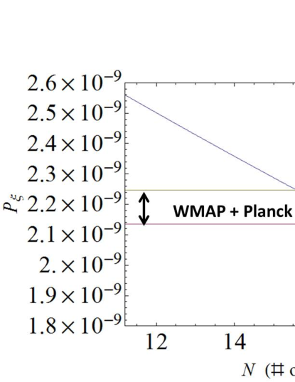
Figure 9: The power spectrum of scalar curvature perturbation between 70 and 60 e-foldings before the end of inflation.

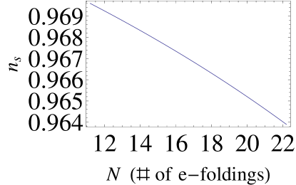
Figure 10: The spectral index of scalar curvature perturbation between 70 and 60 e-foldings before the end of inflation.

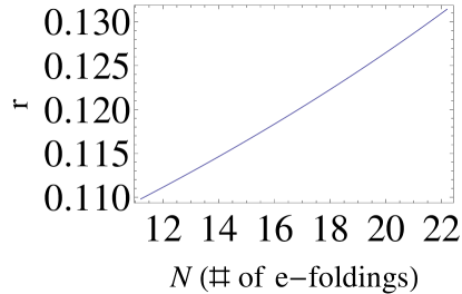
Figure 11: The tensor-to-scalar ratio between 70 and 60 e-foldings before the end of inflation.

4.2 Moduli problem

In this section, we consider the cosmological moduli problem [22] such as moduli-induced gravitino problem [23] and the effect of field oscillation after the inflation. In our both inflation models, the moduli do not induce the SUSY breaking, therefore they do not decay into the gravitino which means that there is no moduli-induced gravitino problem. Even if there is a source of the SUSY breaking in the superpotential, the moduli will not get the F-term because they have large supersymmetric masses.

In addition to the above issues, we have to check the field oscillation after inflationary era, because if the fields other than the inflaton oscillate after the inflation and dominate the universe, they affect the particle cosmology. Since both $\hat{T}^{2}$ and $H_{2}$ have a supersymmetric mass larger than the inflaton mass, we expect that these fields do not oscillate.

By contrast, the stabilzer field $H_{1}$ and the inflaton get the same order of the supersymmetric mass as each other at the vacuum, and then $H_{1}$ could have been stabilized at a point different from its true minimum during the inflation and oscillated around the minimum after the inflation. In the inflationary era however, the mass of $H_{1}$ is given by the Hubble-induced mass proportional to $H_{\rm inf}$ shown in Eqs. (20) and (60) in the small- and the large-field inflation scenarios proposed in the previous Sec. 3 and here in this Sec. 4, respectively.

Therefore, in each scenario, $H_{1}$ is fixed strictly at the origin during and after inflation and does not oscillate and dominate the universe. We further remark that, in the case of small-field inflation discussed in Sec. 3, the imaginary part of modulus Im $T^{1}$ does not oscillate as well if the initial position of Im $T^{1}$ is located at the origin. This is because the Kähler potential has a shift symmetry for the imaginary part and the inflationary dynamics does not involve the imaginary direction.

In order to estimate the effects of supersymmetry breaking on the inflation dynamics, we consider the following superpotential,

$$W =W_{\rm eff}+\Delta W(\hat{T}^{1}),$$ (76)

where $W_{\rm eff}$ represents the superpotential terms responsible for the inflation given in Eq. (50), and $\Delta W(\hat{T}^{1})$ describes the supersymmetry breaking sector, which may involve the inflaton multiplet $\hat{T}^{1}$ in general. We assume that the other fields such as $\hat{T}^{2}$ and $H_{2}$ are stabilized at their supersymmetric minimum. The following analysis can be applied to both the inflation scenarios by replacing the original effective superpotential $W_{\rm eff}$ with the modified one (76) in each scenario. The position of the supersymmetry breaking minimum will be determined by estimating the deviation from the supersymmetric Minkowski minimum (6) by assuming $\langle\Delta W\rangle\sim\langle\partial_{\hat{T}^{1}}(\Delta W\rangle)\ll 1$ (in the unit $M_{\rm Pl}=1$) and employing the reference point method [24].

As the reference point which should be selected as close to the true minimum as possible, we set it in such a way that the following conditions,

$$D_{H_{1}}W|_{\rm ref}=W_{H_{1}}+(K_{\rm eff})_{H_{1}}W=0,$$

$$\hskip 56.9055pt\leftrightarrow c\,\hat{T}^{1}|_{\rm ref}=\text{ln}\frac{J_{L}^{(1)}}{J_{0}^{(1)}}\,\,{\rm and}\;\;H_{1}|_{\rm ref}=0,$$

$$D_{\hat{T}^{1}}W|_{\rm ref}=(K_{\rm eff})_{\hat{T}^{1}}\Delta W,$$ (77)

are satisfied at the point, where the effective Kähler potential $K_{\rm eff}$ is given in Eqs. (8) or (50) for each scenario. Then we expand the field $\varphi=\varphi|_{\rm ref}+\delta\varphi$ for $\varphi=\hat{T}^{1},H_{1}$ and evaluate the deviations $\delta\varphi$ from the reference point $\varphi|_{\rm ref}$. We find the following variations,

$$\delta\hat{T}^{1}={\cal O}\left(\frac{|\Delta W|^{2}}{W_{\hat{T}^{1}H_{1}}}\right),\;\;\;\delta H_{1}=-\frac{(K_{\rm eff})_{\hat{T}^{1}}\Delta W}{W_{\hat{T}^{1}H_{1}}}+{\cal O}(|\Delta W|^{2}),$$ (78)

minimize the scalar potential at their first order, which implies our reference point method is valid if the supersymmetry breaking scale is smaller than the supersymmetric masses of the moduli and stabilizers, that is, $\langle\Delta W\rangle\ll\langle W_{\hat{T}^{1}H_{1}}\rangle$ in the unit $M_{\rm Pl}=1$. In the same way, the F-terms of $\hat{T}^{1}$ and $H_{1}$ at the supersymmetry breaking minimum are estimated as

$$\sqrt{(K_{\rm eff})_{\hat{T}^{1}\bar{\hat{T}}^{1}}}F^{\hat{T}^{1}} =-e^{K_{\rm eff}/2}\sqrt{(K_{\rm eff})_{\hat{T}^{1}\bar{\hat{T}}^{1}}}(K_{\rm eff})^{\hat{T}^{1}\bar{J}}\,\overline{D_{J}W}\simeq{\cal O}\left(\frac{(m_{3/2})^{3}}{(m_{t^{1}})^{2}}\right),$$

$$\sqrt{(K_{\rm eff})_{H_{1}\bar{H}_{1}}}F^{H_{1}} =-e^{K_{\rm eff}/2}\sqrt{(K_{\rm eff})_{H_{1}\bar{H}_{1}}}(K_{\rm eff})^{H_{1}\bar{J}}\,\overline{D_{J}W}\simeq{\cal O}\left(\frac{(m_{3/2})^{3}}{(m_{h_{1}})^{2}}\right),$$ (79)

where $(m_{t^{1}})^{2}$ and $(m_{h_{1}})^{2}$ are given in Eq. (48).

We conclude that if the size of supersymmetry breaking is much smaller than the inflation scale which we assume in this paper, they do not affect the inflation mechanism and the related cosmology after the inflation. In fact, the field $\hat{T}^{1}$ and $H_{1}$ have almost vanishing F-terms which means that the decay channels from $\hat{T}^{1}$ and $H_{1}$ into the gravitino are suppressed and they do not induce the moduli-induced gravitino problem. The coherent oscillation of $H_{1}$ after the inflation is also suppressed, because the amplitude of the oscillation of $H_{1}$,

$$\Delta H_{1}\,\simeq\,\delta H_{1}|_{\rm inf}-\delta H_{1}|_{\rm vac}\,\simeq\,{\cal O}\left(\frac{\Delta W}{H_{\rm inf}}\right)-{\cal O}\left(\frac{\Delta W}{m_{h_{1}}}\right),$$ (80)

is small enough, where $\delta H_{1}|_{\rm inf}$ and $\delta H_{1}|_{\rm vac}$ are the deviations of $H_{1}$ from the supersymmetric Minkowski minimum (6) during the inflation and at the true minimum where the supersymmetry is broken, respectively.

4.3 Reheating temperature

Finally, we show the decay channel and the reheating process after the end of inflation. As shown in Fig. 8, after the inflation, both $\sigma$ and $\tau$ oscillate around the minimum and they decay into particles in the MSSM at the time $t_{\rm dec}^{t^{1}}$ and $t_{\rm dec}^{\phi^{1}}$ respectively where $t^{1}$ and $\phi^{1}$ are the canonically normalized field, $t^{1}\,=\,\sqrt{2(K_{\hat{T}})_{1}}U_{1,1}\sigma+\sqrt{2(K_{\hat{T}})_{1}}U_{1,2}({\rm Re}\,\hat{T}^{2})$, and $\phi^{1}=\sqrt{2(K_{\rm eff})_{\hat{T}^{1}\bar{\hat{T}}^{1}}}\tau$ given in Eqs. (43) and (45), respectively. Note that the eigenvalue $(K_{\hat{T}})_{I^{\prime}}$ and diagonalizing matrix $U_{I^{\prime},J^{\prime}}$ ($I^{\prime}=1,2$) of the Kähler metric are explicitly shown in Appendix A. In the following analysis, we neglect the oscillation of Re $\hat{T}^{2}$ and use the sudden-decay approximation.

The decay time $t_{\rm dec}^{t^{1}}\,=\,1/\Gamma^{t^{1}}$ is the inverse of the decay width of $t^{1}$ which depends on the concrete model of the particle physics. We assume that the modulus $t^{1}$ mainly decay into the gauge boson pairs, $t^{1}\to g^{(a)}+g^{(a)}$, for simplicity. If some matter chiral multiplets $Q$ originating in the hypermultiplet ${\bm{H}}_{\alpha}$ have $U(1)_{I^{\prime}=1,2}$ charges under the $Z_{2}$-odd vector multiplets $V^{I^{\prime}=1,2}$ carrying the inflaton, they induce couplings like $Z(t^{1})|Q|^{2}$ in the Kähler potential where $Z(t^{1})$ is the Kähler metric of $Q$ given by Eq. (4) where the $U(1)_{I^{\prime}=1,2}$ charges are replaced by those of $Q$. These couplings will enhance the inflaton decay width into $Q$ depending on the $U(1)_{I^{\prime}=1,2}$ charge of $Q$. In our model, the decay channel via the F-term of $t^{1}$ is kinematically forbidden, because its vacuum expectation value is negligibly small as mentioned previously. After all, $t^{1}$ mostly decays into the gauge boson pairs with the following decay width,

$$\sum_{a=1}^{3}\Gamma^{t^{1}}(t^{1}\rightarrow g^{(a)}+g^{(a)}) \simeq\sum_{a=1}^{3}\cfrac{N_{G}^{a}}{64\pi}\left\langle\cfrac{\xi_{a}^{1}}{{\rm Re}\,f_{a}}\right\rangle^{2}\left\langle\frac{U_{2,2}}{\sqrt{2(K_{\hat{T}})_{1}}(U_{1,1}U_{2,2}-U_{1,2}U_{2,1})}\right\rangle^{2}\cfrac{m_{t^{1}}^{3}}{M_{\rm Pl}^{2}}$$

$$\simeq 0.86\,\,{\rm GeV},$$ (81)

where $N_{G}^{a}$ is the number of the gauge bosons for the gauge group $G^{a}$ with $a=1,2,3$ representing the three gauge groups in the MSSM, $a=\,U(1)_{Y}$, $SU(2)_{L}$, $SU(3)_{c}$, respectively. We are adopting the numerical values of input parameters, those yield $\langle\sqrt{2(K_{\hat{T}})_{1}}\rangle\simeq 0.86$, $\langle U_{1,1}\rangle\simeq-39.68$, $\langle U_{2,1}\rangle\simeq 0.025$, $\langle U_{1,2}\rangle\,=\,\langle U_{2,2}\rangle\,=\,1$ and $m_{t^{1}}\simeq 1.96\times 10^{13}\,{\rm GeV}$. Especially we set $\xi_{a}^{1}=3.58$ and $\xi_{a}^{I^{\prime}\neq 1}=0$ to realize the correct gauge coupling $\langle f_{a}\rangle\,=\,1/(g_{a})^{2}\simeq 3.73$ at the grand unification scale ($\simeq\,2.0\times 10^{16}[\text{GeV}]$). Because $\Gamma^{t^{1}}(t^{1}\rightarrow g^{(a)}+g^{(a)})$ with $a=1,2,3$ are assumed to be dominant, the total decay width is given by

$$\Gamma^{t^{1}}\simeq\sum_{a=1}^{3}\Gamma^{t^{1}}(t^{1}\rightarrow g^{(a)}+g^{(a)}).$$ (82)

On the other hand, the decay time $t_{\rm dec}^{\phi^{1}}\,=\,1/\Gamma^{\phi^{1}}$ is estimated from the following terms in the Lagrangian,

$${\cal L} \supset-\cfrac{1}{8}{\rm Im}\,f_{a}\epsilon^{\mu\nu\rho\sigma}F^{a}_{\mu\nu}F^{a}_{\rho\sigma}$$

$$=-\cfrac{1}{8}\langle{\rm Im}\,f_{a}\rangle\epsilon^{\mu\nu\rho\sigma}F^{a}_{\mu\nu}F^{a}_{\rho\sigma}-\cfrac{1}{8}\left\langle\cfrac{\partial\,{\rm Im}\,f_{a}}{\partial\phi^{1}}\right\rangle\delta\phi^{1}\,\epsilon^{\mu\nu\rho\sigma}F^{a}_{\mu\nu}F^{a}_{\rho\sigma}.$$ (83)

Then the total decay width of the field $\phi$ is computed as follows,

$$\Gamma^{\phi^{1}}\simeq\sum_{a=1}^{3}\Gamma^{\phi^{1}}(\phi^{1}\rightarrow g^{(a)}+g^{(a)}) \simeq\sum_{a=1}^{3}\cfrac{N_{G}^{a}}{128\pi}\left\langle\cfrac{\xi_{a}^{1}}{\sqrt{(K_{\rm eff})_{\hat{T}^{1}\bar{\hat{T}}^{1}}}{\rm Re}\,f_{a}}\right\rangle^{2}\cfrac{m_{\phi^{1}}^{3}}{M_{\rm Pl}^{2}}$$

$$\simeq 1359\,\,{\rm GeV},$$ (84)

where the given input parameters lead to $\sqrt{(K_{\rm eff})_{\hat{T}^{1}\bar{\hat{T}}^{1}}}\simeq 0.61$ and $m_{\phi^{1}}\simeq 1.96\times 10^{13}\,{\rm GeV}$. Since both the fields $t^{1}$ and $\phi^{1}$ have the almost degenerate supersymmetric masses (59), the differences between $\Gamma^{t^{1}}$ shown in Eq. (81) and $\Gamma^{\phi^{1}}$ in Eq. (84) come from the Kähler metric when the fields $\sigma$ and $\tau$ are diagonalized.

From the expressions (81) and (84), we find the decay time $t^{\phi^{1}}$ is much smaller than $t^{t^{1}}$, i.e., $t^{\phi^{1}}\ll t^{t^{1}}$. It indicates that the inflaton $\phi^{1}$ decay into the radiation faster than the decay of the real part of the modulus $t^{1}$ into the radiation. Then the reheating temperature is estimated by equaling the expansion rate of the universe and the total decay width,

$$\Gamma^{\phi^{1}} \simeq H(T_{R}),$$

$$\Leftrightarrow T_{R} =\left(\cfrac{\pi^{2}g_{\ast}}{90}\right)^{-1/4}\sqrt{\Gamma^{\phi^{1}}M_{\rm Pl}}\simeq 6.8\times 10^{9}\,{\rm GeV},$$ (85)

where $g_{\ast}=915/4$ is the effective degrees of freedom of the radiation at the reheating in the MSSM.

Since $t^{1}$ behaves as the non-relativistic particle after the inflation, its energy density decreases as $a^{-3}$ compared to that of the radiation $a^{-4}$, where $a$ is the scale factor. Thus whether there is a second reheating or not after $t^{1}$ decays depends on the following condition. If the following condition is satisfied, $t^{1}$ dominates the universe and it induces the second reheating,

$$1\leq\frac{\rho_{t^{1}}}{\rho_{R}}\biggl{|}_{T=T_{t^{1}}}\simeq\frac{\rho_{t^{1}}}{\rho_{R}}\biggl{|}_{T=T_{R}}\left(\frac{T_{R}}{T_{t^{1}}}\right),$$ (86)

where $\rho_{t^{1}}$ and $\rho_{R}$ are the energy densities of $t^{1}$ and the radiation, respectively, and $T_{t^{1}}$ is the decay temperature of $t^{1}$ given by

$$T_{t^{1}} =\left(\cfrac{\pi^{2}g_{\ast}}{90}\right)^{-1/4}\sqrt{\Gamma^{t^{1}}M_{\rm Pl}}\simeq 1.7\times 10^{8}\,{\rm GeV}.$$ (87)

After the inflation, the field $t^{1}$ and the inflaton $\phi^{1}$ oscillate at the same time and the difference between them is only the size of the decay width. Thus we expect that the amplitude of $\Delta t^{1}$ is small enough at the time $t^{\phi^{1}}$ and the energy density $\rho_{t^{1}}\simeq m_{t^{1}}^{2}(\Delta t^{1})^{2}$ is neglected compared to that of the radiation $\rho_{R}^{1/4}\,=\,2\times 10^{10}\,{\rm GeV}$. It follows that the above condition (86) is not satisfied, and then the second reheating does not occur.

Finally we comment on the one-loop corrections to the moduli Kähler potential given by Eq. (33). Although the loop correction to the effective Kähler potential depends on the moduli Re $\hat{T}^{I^{\prime}}$ with $I^{\prime}=1,2$ via the Norm function ${\cal N}$ shown in Eq (41), the Re $\hat{T}^{1}$-dependence of the potential is similar to that of the tree-level Kähler potential. Since the scalar potential also diverges in the limit $b\,{\rm Re}\,\hat{T}^{1}\rightarrow{\rm Re}\,\hat{T}^{2}$ due to the behavior of the following factor in this limit,

$$e^{K_{\rm eff}}\simeq\frac{e^{1/(32\pi^{2}{\cal N})}}{{\cal N}}\rightarrow\infty,$$ (88)

the modulus ${\rm Re}\,\hat{T}^{1}$ is not destabilized during and after the inflation. Such a behavior implies that the field Re $\hat{T}^{1}$ remains stabilized during the inflation, which is considered as the single-field inflation with the imaginary part of modulus identified as the inflaton.

5 Conclusion

In this paper, we proposed the effective mechanism to realize successful inflation to explain the cosmological observations based on the 5D supergravity models on $S^{1}/Z_{2}$. In our framework, we can realize both the small- and the large-field inflation scenarios, where the role of inflaton is played by a linear combination of the moduli appearing after compactifying the fifth direction. These two inflation scenarios would be compatible with numerous particle physics models constructed in 5D.

In the case of the small-field inflation, the real part of the light modulus, Re $T^{1}$, is considered as the inflaton and the inflaton potential is induced by the superpotential of the stabilizer field, $H_{1}$, which has a localized wavefunction in the fifth dimension. This small-field inflaton potential is consistent with WMAP and Planck data [1], although they cannot explain the large tensor-to-scalar ratio reported by BICEP2 [2]. We have also studied the particle cosmology in this inflationary scenario and find that there is no moduli and gravitino over production.

We further presented a different setup within the same 5D supergravity framework, realizing the large-field inflation which produces the sizable tensor-to-scalar ratio consistent with the results from BICEP2. In this scenario, the two light pairs of moduli and stabilizer fields ($\hat{T}^{I^{\prime}},H_{i}$) with $I^{\prime},i=1,2$ are introduced and the inflaton is identified as the imaginary part of the lightest modulus Im $\hat{T}^{1}$. The moduli potential is induced by the superpotential of the stabilizer fields as in the small-field scenario. The inflaton potential is similar to the one of natural inflation [18], but in our framework, the axion decay constant is given by the $U(1)$ charges originated from the $Z_{2}$-odd vector multiplets carrying the inflaton field. Both the inflation scenarios proposed in this paper are free from the $\eta$ problem which is peculiar to the inflationary dynamics in the four-dimensional ${\cal N}=1$ supergravity models.

In the large-field scenario, when the imaginary part of the modulus rolls down in its potential, the real part of the modulus will be destabilized because there is a runaway direction in its potential in general. However, in our model, the real part of the modulus, Re $\hat{T}^{1}$, can be stabilized during the inflation, because of the potential barrier is produced by the real part of the heavier modulus, Re $\hat{T}^{2}$, in the Kähler potential. After the inflation, both the imaginary and the real part of the modulus, Im$\,\hat{T}^{1}$ and Re$\,\hat{T}^{1}$ oscillate but only the inflaton Im $\hat{T}^{1}$ reheats the universe. The reheating temperature is estimated from the decay width of the inflaton into the gauge boson pairs. The stabilizer fields are also fixed at the origin during (-and after-) the inflation by the Hubble-induced and their own supersymmetric masses. Therefore there is no cosmological moduli problem also in the large-field scenario.

Both the proposed inflation scenarios are insensitive to the supersymmetry breaking required by the particle phenomenology, if the breaking scale is lower than the inflation scale. This is because the large supersymmetric masses are provided from the superpotential of charged stabilizer fields, those are controlled by the $U(1)$ charges under the 5D vector multiplets carrying the moduli. The branching ratio of the moduli decaying into gravitino is suppressed due to such the supersymmetric masses of moduli. The field in the supersymmetry breaking sector may oscillate after the inflation if the size of supersymmetry breaking is smaller than the inflation scale. The further model building of the particle cosmology including the concrete matter sectors remains as a future work.

The moduli potential as well as their kinetic terms are strictly constrained by the symmetries in higher-dimensional spacetime, although the moduli behave as Lorentz scalars in the four-dimensional spacetime with the extra-dimensions compactified. For the inflationary dynamics proposed in this paper, the $U(1)_{I^{\prime}}$ symmetries played essential roles, those generate the localized wavefunctions of charged stabilizer zero-modes and then yield the suitable moduli potential. It would be possible that the 5D supergravity studied in this paper is derived as the 5D effective theory of supergravities in more-than-five dimensional spacetime, superstrings in ten-dimensions and the M-theory in eleven-dimensions [14]. In such cases, the coefficients $C_{I,J,K}$ in the norm function will be related to the geometric structure of the internal space (e.g., the intersection numbers of Calabi-Yau manifold) and the above $U(1)_{I^{\prime}}$ symmetries might originate from certain local symmetries with the gauge fields in the higher-dimensional spacetime. Our 5D models not only work well observationally, but also would be theoretically instructive and extensible from the above points of view.

Acknowledgement

The authors would like to thank T. Higaki, Y. Sakamura and Y. Yamada for useful discussions and comments. The work of H. A. was supported in part by the Grant-in-Aid for Scientific Research No. 25800158 from the Ministry of Education, Culture, Sports, Science and Technology (MEXT) in Japan. H. O. was supported in part by a Grant-in-Aid for JSPS Fellows No. 26-7296 and a Grant for Excellent Graduate Schools from the MEXT in Japan.

Appendix A The canonical normalization in the large-field model

As we have seen in Sec. 4, the moduli stabilization mechanism involves sizable moduli mixings in the Kähler metric and we have to canonically normalize the moduli to estimate their masses. In this appendix, we show the eigenvalue $(K_{\hat{T}})_{I^{\prime}}$ and the diagonalizing matrix $U_{I^{\prime}\bar{J}^{\prime}}$ of the Kähler metric $K_{I^{\prime}\bar{J}^{\prime}}$.

The Kähler metric in the effective Kähler potential (34) derived from the norm function (41) with $a=1$ is given by

$$(K_{\rm eff})_{I^{\prime},\bar{J}^{\prime}}\,=\,\begin{pmatrix}\left(\frac{1}{2\sigma^{1}}\right)^{2}+\frac{1}{2}\left(\frac{b}{\sigma^{2}-b\,\sigma^{1}}\right)^{2}&-\frac{b}{2\left(\sigma^{2}-b\,\sigma^{1}\right)^{2}}\\ -\frac{b}{2\left(\sigma^{2}-b\,\sigma^{1}\right)^{2}}&\frac{1}{2\left(\sigma^{2}-b\,\sigma^{1}\right)^{2}}.\end{pmatrix},$$ (89)

where we define $\sigma^{I^{\prime}}\equiv{\rm Re}\,\hat{T}^{I^{\prime}}$ with $I^{\prime}=1,2$ in this appendix. Then the eigenvalues of Kähler metric (89) are estimated as

$$(K_{\hat{T}})_{1}\, =\,\frac{(2+3b^{2})(\sigma^{1})^{2}-2b\,\sigma^{1}\sigma^{2}+(\sigma^{2})^{2}}{8(\sigma^{1})^{2}(\sigma^{2}-b\,\sigma^{1})^{2}}+\frac{\sqrt{g(\sigma^{1},\sigma^{2})}}{8(\sigma^{1})^{2}(\sigma^{2}-b\,\sigma^{1})^{2}},$$

$$(K_{\hat{T}})_{2}\, =\,\frac{(2+3b^{2})(\sigma^{1})^{2}-2b\,\sigma^{1}\sigma^{2}+(\sigma^{2})^{2}}{8(\sigma^{1})^{2}(\sigma^{2}-b\,\sigma^{1})^{2}}-\frac{\sqrt{g(\sigma^{1},\sigma^{2})}}{8(\sigma^{1})^{2}(\sigma^{2}-b\,\sigma^{1})^{2}},$$

$$g(\sigma^{1},\sigma^{2}) \equiv(4+4b^{2}+9b^{4})(\sigma^{1})^{4}+4b(2-3b^{2})(\sigma^{1})^{3}\sigma^{2}$$

$$\hskip 16.0pt+2(5b^{2}-2)(\sigma^{1})^{2}(\sigma^{2})^{2}-4b\,\sigma^{1}\,(\sigma^{2})^{3}+(\sigma^{2})^{4}.$$ (90)

The diagonalizing matrix of the Kähler metric (89) is given by

$$U\, =\,\begin{pmatrix}U_{1,1}&1\\ U_{2,1}&1\end{pmatrix},$$

$$U_{1,1} =\frac{(2-3b^{2})(\sigma^{1})^{2}+2b\,\sigma^{1}\sigma^{2}-(\sigma^{2})^{2}}{4b\,(\sigma^{1})^{2}}-\frac{\sqrt{g(\sigma^{1},\sigma^{2})}}{4b\,(\sigma^{1})^{2}},$$

$$U_{2,1} =\frac{(2-3b^{2})(\sigma^{1})^{2}+2b\,\sigma^{1}\sigma^{2}-(\sigma^{2})^{2}}{4b\,(\sigma^{1})^{2}}+\frac{\sqrt{g(\sigma^{1},\sigma^{2})}}{4b\,(\sigma^{1})^{2}}.$$ (91)

References

- [1] P. A. R. Ade et al. [Planck Collaboration], arXiv:1303.5076 [astro-ph.CO].
- [2] P. A. R. Ade et al. [BICEP2 Collaboration], arXiv:1403.3985 [astro-ph.CO].
- [3] M. Zucker, Nucl. Phys. B 570 (2000) 267 [hep-th/9907082]; M. Zucker, JHEP 0008 (2000) 016 [hep-th/9909144]; M. Zucker, Phys. Rev. D 64 (2001) 024024 [hep-th/0009083]; M. Zucker, Fortsch. Phys. 51 (2003) 899.
- [4] T. Kugo and K. Ohashi, Prog. Theor. Phys. 105 (2001) 323 [hep-ph/0010288], T. Fujita and K. Ohashi, Prog. Theor. Phys. 106 (2001) 221 [hep-th/0104130], T. Fujita, T. Kugo and K. Ohashi, Prog. Theor. Phys. 106 (2001) 671 [hep-th/0106051], T. Kugo and K. Ohashi, Prog. Theor. Phys. 108 (2002) 203 [hep-th/0203276].
- [5] H. Abe and Y. Sakamura, Phys. Rev. D 75 (2007) 025018 [hep-th/0610234].
- [6] H. Abe and Y. Sakamura, JHEP 0410 (2004) 013 [hep-th/0408224].
- [7] F. Paccetti Correia, M. G. Schmidt, Z. Tavartkiladze and , Nucl. Phys. B 709 (2005) 141 [hep-th/0408138],
- [8] N. Arkani-Hamed and M. Schmaltz, Phys. Rev. D 61 (2000) 033005 [hep-ph/9903417], D. E. Kaplan and T. M. P. Tait, JHEP 0006 (2000) 020 [hep-ph/0004200].
- [9] H. Abe and Y. Sakamura, Phys. Rev. D 79 (2009) 045005 [arXiv:0807.3725 [hep-th]]; H. Abe, H. Otsuka, Y. Sakamura and Y. Yamada, Eur. Phys. J. C 72 (2012) 2018 [arXiv:1111.3721 [hep-ph]].
- [10] L. Randall and R. Sundrum, Phys. Rev. Lett. 83 (1999) 3370 [hep-ph/9905221].
- [11] N. Maru and N. Okada, Phys. Rev. D 70 (2004) 025002 [hep-th/0312148].
- [12] H. Abe and Y. Sakamura, Nucl. Phys. B 796 (2008) 224 [arXiv:0709.3791 [hep-th]].
- [13] A. A. Starobinsky, Phys. Lett. B 91 (1980) 99.
- [14] A. Lukas, B. A. Ovrut, K. S. Stelle and D. Waldram, Phys. Rev. D 59 (1999) 086001 [hep-th/9803235], A. Lukas, B. A. Ovrut, K. S. Stelle and D. Waldram, Nucl. Phys. B 552 (1999) 246 [hep-th/9806051].
- [15] C. P. Burgess, J. M. Cline, H. Stoica and F. Quevedo, JHEP 0409 (2004) 033 [hep-th/0403119].
- [16] A. R. Liddle and D. H. Lyth, Phys. Rept. 231 (1993) 1 [astro-ph/9303019].
- [17] Y. Sakamura, Nucl. Phys. B 873 (2013) 165 [Erratum-ibid. B 873 (2013) 728] [arXiv:1302.7244 [hep-th]], Y. Sakamura and Y. Yamada, JHEP 1311 (2013) 090 [arXiv:1307.5585 [hep-th]].
- [18] K. Freese, J. A. Frieman and A. V. Olinto, Phys. Rev. Lett. 65 (1990) 3233.
- [19] K. Freese and W. H. Kinney, arXiv:1403.5277 [astro-ph.CO].
- [20] A. D. Linde, Phys. Lett. B 129 (1983) 177.
- [21] J. E. Kim, H. P. Nilles and M. Peloso, JCAP 0501 (2005) 005 [hep-ph/0409138].
- [22] D. H. Lyth and E. D. Stewart, Phys. Rev. D 53 (1996) 1784 [hep-ph/9510204].
- [23] M. Endo, K. Hamaguchi and F. Takahashi, Phys. Rev. Lett. 96 (2006) 211301 [hep-ph/0602061].
- [24] H. Abe, T. Higaki, T. Kobayashi and Y. Omura, Phys. Rev. D 75 (2007) 025019 [hep-th/0611024].