Model-independent determination of the magnetic radius of the proton from spectroscopy of ordinary and muonic hydrogen

Abstract

To date the magnetic radius of the proton has been determined only by means of electron-proton scattering, which is not free of controversies. Any existing atomic determinations are irrelevant because they are strongly model-dependent. We consider a so-called Zemach contribution to the hyperfine interval in ordinary and muonic hydrogen and derive a self-consistent model-independent value of the magnetic radius of the proton. More accurately, we constrain not a value of the magnetic radius by itself, but its certain combination with the electric-charge radius of the proton, namely, $R_{E}^{2}+R_{M}^{2}$. The result from the ordinary hydrogen is found to be $R_{E}^{2}+R_{M}^{2}=1.35(12)\;{\rm fm}^{2}$, while the derived muonic value is $1.49(18)\;{\rm fm}^{2}$. That allows us to constrain the value of the magnetic radius of proton $R_{M}=0.78(8)\;{\rm fm}$ at the 10% level.

I Introduction

While a discrepancy between results on determination of the electric charge radius of the proton has lately attracted attention of theoreticians and experimentalists, a controversy in determination of the magnetic radius is rather in shadow. The situation is summarized in Fig. 1. The proton charge radius has already been discussed in efit , which is referred here as paper I. This paper is a direct continuation of paper I and we do not reproduce here any plots or equations from there.

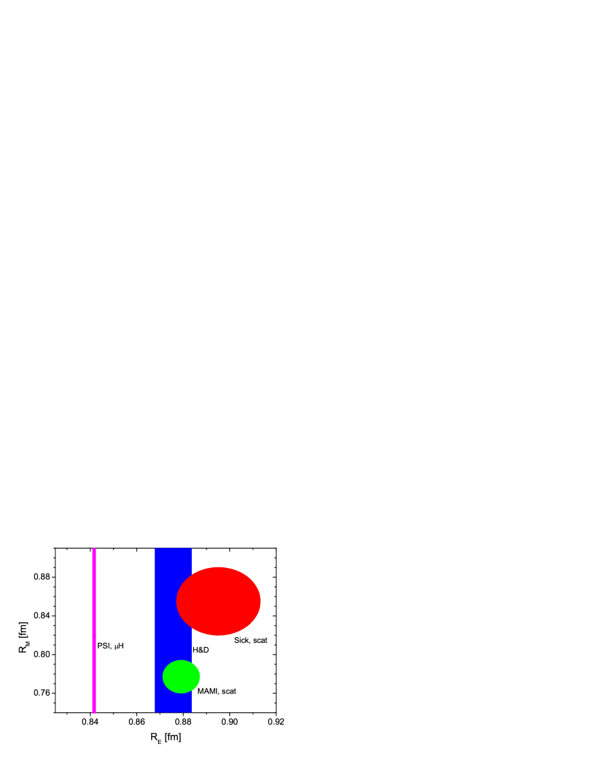
Figure 1: Determination of the rms proton charge and magnetic radii. (Sick sick has evaluated all the world data, but MAMI results mami . Other evaluations of those data produced similar results (see, e.g., zhan ).) Ellipses for electron-proton scattering should be somewhat turned from a pure horizontal position because of a small correlation between $R_{E}$ and $R_{M}$. For details see my_adp ; my_ufn .

A stronger interest to the situation with the electric charge radius $R_{E}$ is due to a broader variety of the data and more important applications, such as determination of the Rydberg constant. While in the case of the magnetic radius $R_{M}$ there is a discrepancy between two scattering results mami ; sick , the set of results for $R_{E}$ also includes the spectroscopic data on hydrogen and deuterium codata2010 and on muonic hydrogen Nature ; Science .

The contradiction between different values of $R_{M}$ is rather serious, while reading the published results literally. To certain extent it is expected that the discrepancy is partly due to different treatment of the proton polarizability contribution comm ; resp . However, that may remove only a part of the discrepancy.

The spectroscopic data and, in particular, results on the hyperfine-structure (HFS) interval in hydrogen ($1s$) and muonic hydrogen ($2s$) Science , may present a source for an independent extraction of $R_{M}$, however, at present there is no model-independent constraints on $R_{M}$ from the HFS interval in muonic or ordinary hydrogen. Values published from time to time are deduced from models of the proton form factors, but there has been no realistic model of the proton developed to date.

Any comparison of ‘pure’ QED theory with the experimental results on hydrogen has been ‘contaminated’ for decades by the presence of certain proton finite-size and polarizability contributions. While the experimental value of the $1s$ interval in hydrogen had been for a while among the most accurately measured physical quantities, the most sensitive QED tests for the HFS-interval theory has been performed not with the $1s$ interval in hydrogen, but with quantities free of the influence of the nuclear structure. Such quantities have been provided by a study of leptonic atoms, such as muonium or positronium. Another opportunity is a comparison of the $1s$ and $2s$ HFS intervals measured with the same atom. Details of those QED tests with the HFS can be found, e.g., in review my_rep .

Here we explore a related question. The main purpose of this note is to estimate the constraints on the magnetic radius of the proton, $R_{M}$, from the hyperfine splitting in muonic and ordinary hydrogen. If the proton polarizability contributions are known with a sufficient accuracy, we can experimentally determine the value of the proton finite-size contribution by a comparison of the theory and experiment. Such a contribution must be sensitive to the distribution of both electric charge and magnetic moment inside the proton. Considering that contribution in an appropriate way, we intend to extract a constraint on a certain combination of $R_{E}$ and $R_{M}$.

While the QED effects are well understood (see, e.g., my_rep ), the total theoretical accuracy for the HFS interval in both muonic and ordinary hydrogen is completely determined by the proton-structure terms, namely, by the elastic two-photon contribution and by the proton polarizability correction. In case of hydrogen the experimental uncertainty is negligible, while for $\mu$H it is compatible with and somewhat higher than the theoretical one.

As for calculation of the elastic term, its dominant part can be found in the external field approximation. We have to deal with integral

$$I_{1}^{\rm EM} \equiv \int_{0}^{\infty}{\frac{dq}{q^{2}}}\left[\frac{G_{E}(q^{2})G_{M}(q^{2})}{\mu_{p}}-1\right]\;,$$ (1)

which determines the dominant proton-finite-size contributions into the HFS interval in ordinary and muonic hydrogen

$$\Delta E_{\rm HFS}(ns) = \frac{8(Z\alpha)m_{r}}{\pi n^{3}}E_{F}\,I_{1}^{\rm EM}\;,$$ (2)

where $E_{F}$ is the so-called Fermi energy, $m_{r}$ is the reduced mass of a bound electron (in hydrogen) or muon (in muonic hydrogen) and $\mu_{p}=2.7928...$ is the proton magnetic moment in units of the nuclear magnetons. For available experimental data $n=1$ for ordinary hydrogen (see, e.g., a summary on the $1s$ HFS interval in 1s ) and $n=2$ for muonic hydrogen Science . The other notation used for the integral under question presents it in terms of the so-called Zemach radius (or the first Zemach momentum)

$$\langle r\rangle_{Z} = -\frac{4}{\pi}I_{1}^{\rm EM}\;.$$ (3)

We have no direct experimental knowledge on the integrand in (1), which consists of the subtracted form factors of the proton, ${G_{E}(q^{2})G_{M}(q^{2})}/{\mu_{p}}-1$. In particular, the accurate data fail at low momenta, which essentially contribute to the integral. Everything used in the integrand was a result of certain fitting rather than direct measurements. (We in part explore here ideas presented previously in pla and developed in paper I.)

The situation with the integrand in (1) is illustrated in Fig. 2, where various fractional contributions to the integrand are estimated from the dipole model and presented as a function of $q/\Lambda$. The red dot-dashed line is for the subtraction term with unity. The blue solid line is for the $G_{E}G_{M}$ term, which is related to the data. The integral is fast convergent at high $q$. At low $q$, say below $0.3\Lambda$, the data contribution produces a large uncertainty and any successful result for the Zemach contribution obtained previously was based on a certain, sometimes unrealistic, model.

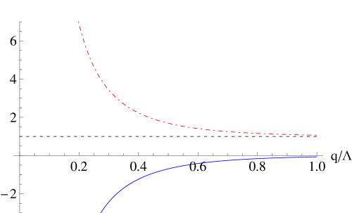
Figure 2: Fractional contributions to the integrand in (1) as a function of $q/\Lambda$ as follows from the dipole model. The red dot-dashed line is the subtraction term with unity and the blue solid line is the $G_{E}G_{M}$ term, i.e. for the data (cf. pla ; efit ).

We are going to split the integration into two parts:

$$I=\int_{0}^{\infty}{{dq}{...}}\equiv I_{<}+I_{>}\equiv\int_{0}^{q_{0}}{{dq}{...}}+\int_{q_{0}}^{\infty}{{dq}{...}}$$ (4)

which are to be treated differently (cf. pla ; efit ).

For higher momenta, we will use direct experimental data (or rather their realistic approximation). The accuracy of the form factors is roughly 1%. The integral over the direct data is indeed singular at $q_{0}\to 0$, because the experimental values of $G_{E}(0)$ and $G_{M}(0)/\mu_{p}$ are not equal to unity exactly — they are only consistent with unity within the uncertainty, which produces the singularity. The smaller is $q_{0}$ the larger is the uncertainty of the related integral.

On the other hand, we can expand the form factors at low momentum

$$\frac{G_{E}(q^{2})G_{M}(q^{2})}{\mu_{p}}=A+Bq^{2}+Cq^{4}+...\\$$

Some contributions into $I_{1<}^{\rm EM}$ vanish because of the subtraction and the uncertainty comes from the remaining terms. The smaller is $q_{0}$ the smaller is the uncertainty. Here, $A=1$ and $B=-(R_{E}^{2}+R_{M}^{2})/6$. The $B$ contribution to $I_{1<}^{\rm EM}$

$$I_{1}^{\rm R}=-\frac{R_{E}^{2}+R_{M}^{2}}{6}q_{0}$$ (5)

is to be treated separately. That is the ‘signal’ that we use to constrain $R_{E}^{2}+R_{M}^{2}$. The leading remaining term is the $C$ term, which is responsible for the uncertainty.

The idea is to apply a certain model to estimate the uncertainties and to find a value of $q_{0}$, which corresponds to the smallest uncertainty possible (cf. paper I).

Concluding on the model to estimate the uncertainty, we note that the dipole form factor is a reasonable estimation for the form factors as far as we discuss general features, but not any accurate particular value. So, we can, e.g., set for $G_{E}G_{M}/\mu_{p}$

$$C = bC^{\rm dip}\;,$$

$$C^{\rm dip} = \frac{10}{\Lambda^{4}}\;,$$ (6)

and estimate the $b$ coefficient as $b=1\pm 1$ (cf. efit ). Here, we use for various preliminary estimations the standard dipole model

$$G_{\rm dip}(q^{2})=\left(\frac{\Lambda^{2}}{q^{2}+\Lambda^{2}}\right)^{2}$$

and apply for numerical evaluations $\Lambda^{2}=0.71\,{\rm GeV}^{2}$, which corresponds to $R_{\rm dip}=0.811\;$fm.

II Consideration within the dipole model

Let us perform an evaluation of $I_{1}^{\rm EM}$ following the consideration of $I_{3}^{\rm E}$ in paper I.

The complete dipole value useful for further estimation of the fractional uncertainties is

$$I_{1}^{\rm dip} = \int_{0}^{\infty}{\frac{dq}{q^{2}}}\left[\left(G_{d}(q^{2})\right)^{2}-1\right]$$ (7)

$$= -\frac{35}{32}\frac{\pi}{\Lambda}$$

$$\simeq -4.08\;{\rm GeV}^{-1}$$

$$\simeq -0.805\;{\rm fm}\;.$$

III Splitting the integral into parts

As we intend to split the integral into two parts, let us start with the higher-momentum part

$$I_{1>}^{\rm EM} = \int_{q_{0}}^{\infty}{\frac{dq}{q^{2}}}\left[\frac{G_{E}(q^{2})G_{M}(q^{2})}{\mu_{p}}-1\right]$$ (8)

$$= \int_{q_{0}}^{\infty}{\frac{dq}{q^{2}}\frac{G_{E}(q^{2})G_{M}(q^{2})}{\mu_{p}}}-\frac{1}{q_{0}}\;.$$

Its uncertainty is estimated, by considering the part of the integral, singular at the limit $q_{0}\to 0$. The result is

$$\delta I_{1>}^{\rm EM} = \delta\int_{q_{0}}^{\infty}{\frac{dq}{q^{2}}}\frac{G_{E}(q^{2})G_{M}(q^{2})}{\mu_{p}}$$ (9)

$$\simeq \delta\int_{q_{0}}^{\infty}{\frac{dq}{q^{2}}}\frac{G_{E}(q_{0}^{2})G_{M}(q_{0}^{2})}{\mu_{p}}$$

$$= \frac{1}{\nu\Lambda}\frac{2\delta G(q_{0}^{2})}{G(q_{0}^{2})}\left(\frac{1}{1+\nu^{2}}\right)^{4}$$

or

$$\frac{\delta I_{1>}^{\rm EM}}{-I_{1}^{\rm dip}}\simeq\frac{0.0058}{\nu}\left(\frac{1}{1+\nu^{2}}\right)^{4}\;,$$

where $\nu=q_{0}/\Lambda$ and we suggest for our estimations that both electric and magnetic form factors roughly follow the standard dipole fit and we experimentally know both of them within 1% uncertainty

$$\frac{\delta G(q_{0}^{2})}{G(q_{0}^{2})}\equiv\frac{\delta G_{E}(q_{0}^{2})}{G_{E}(q_{0}^{2})}\simeq\frac{\delta G_{M}(q_{0}^{2})}{G_{M}(q_{0}^{2})}\simeq 1\%\;.$$

Here we apply the dipole values for estimation of absolute and fractional uncertainties (cf. paper I).

Meanwhile, at low momenta, we find

$$I_{1<}^{\rm EM} = \int_{0}^{q_{0}}{\frac{dq}{q^{2}}}\left[\frac{G_{E}(q^{2})G_{M}(q^{2})}{\mu_{p}}-1\right]$$ (10)

$$= -\frac{R_{E}^{2}+R_{M}^{2}}{6}q_{0}+\frac{10}{3}b\frac{q_{0}^{3}}{\Lambda^{4}}\;,$$

where $b$ was defined above.

IV The extraction: a general consideration

Combining an experimental value, QED contributions and a polarizability correction we obtain

$$I_{1}^{\rm exp} = \frac{\pi n^{3}}{8(Z\alpha)m_{r}E_{F}}\left(E_{\rm HFS}^{\rm exp}-E_{\rm HFS}^{\rm QED}-\Delta E_{\rm HFS}^{\rm polarizability}\right)$$ (11)

$$= \frac{\pi}{8(Z\alpha)m_{r}}\frac{\left(E_{\rm HFS}^{\rm exp}-E_{\rm HFS}^{\rm QED}-\Delta E_{\rm HFS}^{\rm polarizability}\right)}{E_{\rm HFS}}$$

where we noted that $E_{\rm HFS}\simeq E_{F}/n^{3}$ with accuracy sufficient for the denominator. Alternatively, we can write

$$\langle r\rangle_{Z}^{\rm exp}=-\frac{1}{2(Z\alpha)m_{r}}\frac{\left(E_{\rm HFS}^{\rm exp}-E_{\rm HFS}^{\rm QED}-\Delta E_{\rm HFS}^{\rm polarizability}\right)}{E_{\rm HFS}}\;.$$ (12)

Indeed, there are also some higher-order proton-structure corrections, such as a recoil part of the two-photon exchange. We assume that they are included if necessary in the QED or polarizability term.

Often in some papers, they present $\langle r\rangle_{Z}^{\rm exp}$ rather than $I_{1}^{\rm exp}$. Some ‘experimental’ values of $I_{1}^{\rm exp}$ are summarized in Table 1. Any ‘experimental’ value is a result of an extraction procedure that deeply involves theory and, in particular, a calculation of the proton polarizability, which dominates in the uncertainty budget for hydrogen and produces an uncertainty comparable with the measurement uncertainty for muonic hydrogen.

Atom	State	$\langle r\rangle_{Z}$	$I_{1}^{\rm exp}$	$\delta I_{1}^{\rm exp}/I_{1}^{\rm exp}$	Ref.
H	$1s$	1.047(16) fm	$-4.17(6)\,{\rm GeV}^{-1}$	1.5%	h30
H	$1s$	1.037(16) fm	$-4.13(6)\,{\rm GeV}^{-1}$	1.5%	h31
$\mu$H	$2s$	1.082(37) fm	$-4.31(15)\,{\rm GeV}^{-1}$	3.4%	Science

Table 1: Some ‘experimental’ values for $I_{1}$. For numerical evaluations in this paper we use for hydrogen the value from h30 .

Meantime, according to our theoretical consideration

$$I_{1}^{\rm th} = -\frac{R_{E}^{2}+R_{M}^{2}}{6}q_{0}+\frac{10}{3}\bigl{(}1\pm 1\bigr{)}\frac{q_{0}^{3}}{\Lambda^{4}}+I_{1>}^{\rm EM}$$ (13)

$$= -\frac{R_{E}^{2}+R_{M}^{2}}{6}q_{0}+\left(I_{1}^{\rm EM}-I_{1}^{\rm R}\right)\;,$$

and thus we arrive at

$$R_{E}^{2}+R_{M}^{2}=-\frac{6}{q_{0}}\Bigl{(}I_{1}^{\rm exp}-\left(I_{1}^{\rm EM}-I_{1}^{\rm R}\right)\Bigr{)}\;.$$

V The extraction: the uncertainty budget and its optimization

It may be useful to introduce the fractional uncertainty of $R_{E}^{2}+R_{M}^{2}$

$$\delta_{2R}=\frac{\delta\bigl{(}R_{E}^{2}+R_{M}^{2}\bigr{)}}{R_{E}^{2}+R_{M}^{2}}\;.$$

Since roughly $R_{E}\approx R_{M}\approx R_{\rm dip}$, a somewhat different value

$$\delta^{\prime}_{2R} = \frac{\delta\bigl{(}R_{E}^{2}+R_{M}^{2}\bigr{)}}{2R_{\rm dip}^{2}}$$ (14)

is roughly equal to $\delta_{2R}$, but easier to handle. It is sufficient to minimize the uncertainty of determination of $R_{E}^{2}+R_{M}^{2}$.

It is equal to the rms sum of partial uncertainties, which are

$$\delta^{\prime}_{\rm exp} = \frac{6}{q_{0}}\frac{I_{1}^{\rm dip}}{2R_{\rm dip}^{2}}\frac{\delta I_{1}^{\rm exp}}{I_{1}^{\rm dip}}\;,$$

$$\delta^{\prime}_{<} = \frac{6}{q_{0}}\frac{I_{1}^{\rm dip}}{2R_{\rm dip}^{2}}\frac{\delta I_{1<}^{\rm EM}}{I_{1}^{\rm dip}}\;,$$

$$\delta^{\prime}_{>} = \frac{6}{q_{0}}\frac{I_{1}^{\rm dip}}{2R_{\rm dip}^{2}}\frac{\delta I_{1>}^{\rm EM}}{I_{1}^{\rm dip}}\;.$$

With

$$R_{\rm dip}^{2}=\frac{12}{\Lambda^{2}}$$

and

$$\frac{6}{\Lambda}\frac{-I_{1}^{\rm dip}}{2R_{\rm dip}^{2}}=0.8590...\;,$$

we obtain

$$\delta^{\prime}_{<} = 0.83\,\nu^{2}\;,$$

$$\delta^{\prime}_{>} = \frac{0.0050}{\nu^{2}}\left(\frac{1}{1+\nu^{2}}\right)^{4}\;.$$

To find $\delta_{\rm exp}$, we have to utilize the results from Table 1

$$\delta^{\prime}_{\rm exp,\;H} = \frac{0.013}{\nu}\;,$$

$$\delta^{\prime}_{{\rm exp,\;}\mu{\rm H}} = \frac{0.031}{\nu}\;,$$

where for ordinary hydrogen we use the result from h30 .

With the uncertainty determined, let us consider behavior of the uncertainty as a function of $\nu=q_{0}/\Lambda$. All the partial uncertainties as well as the total one as a function of $\nu$ are plotted in Fig. 3 both for ordinary (top) and muonic (bottom) hydrogen.

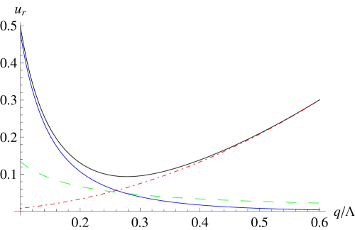
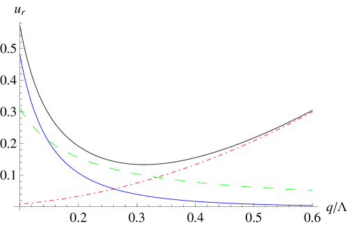
Figure 3: The total fractional uncertainty $\delta^{\prime}_{2R}$ (a black solid line) as the rms sum of sources listed above as a function of $\nu=q_{0}/\Lambda$. The partial uncertainties are also presented. The top plot is for ordinary hydrogen, while the bottom one is for $\mu$H. The red dot-dashed lines are for the uncertainty of the low-momentum part of the $I_{1}^{\rm EM}$ integral and the blue solid ones are for high-momentum contribution to the uncertainty budget; the ‘experimental’ uncertainties, which are different for muonic and ordinary hydrogen (see Table 1), are presented with green dashed lines.

The optimal values, which minimize the uncertainty, and the partial contributions to the total uncertainty for those values are collected in Table 2.

Atom	Best $\nu$	Best $q_{0}$	$\delta^{\prime}_{2R}$	$\delta^{\prime}_{\rm exp}$	$\delta^{\prime}_{<}$	$\delta^{\prime}_{>}$	Scat	Scat∗
H	0.278	0.234 GeV	9.4%	4.8%	6.4%	4.8%	1.3%	3.2%
$\mu$H	0.312	0.263 GeV	13.3%	9.9%	8.1%	3.5%	0.9%	2.0%

Table 2: Parameters for evaluation of the fractional of uncertainties and fractional scatter of the results (see below). The scatter of the results from a fit to fit is used to control accuracy. It is not included into the error budget. Scatter is for the scatter of the results without fits from bo1994 and scatter^∗ is for the scatter including the fits from bo1994 (see below for detail).

VI The fits of the proton form factors

Now we are to find $I_{1}^{\rm EM}-I_{1}^{\rm R}$ by integration over the data. As in paper I, we use for that a certain set of fits.

As an approximation we utilize the fits for the proton form factors $G_{E}$ and $G_{M}$ from Arrington and Sick, 2007 as2007 , Kelly, 2004 kelly , Arrington et al., 2007 am2007 , Alberico et al., 2009 ab2009 , Venkat et al., 2011 va2011 , and from Bosted, 1995 bo1994 . The details of the fits for the electric form factor are presented in efit , while for the magnetic one they are summarized in Appendix A.

Two of the fits for $G_{M}$ are with so-called chain fractions, five are with Padé approximations with polynomials in $q^{2}$, and one is a Padé approximation with polynomials in $q$.

As well as in case of a pure electric integral in efit , the fit (24) of Bosted bo1994 is perfect for the tests. It is a Padé approximation with polynomials in $q$, not in $q^{2}$. It definitely has a low-momentum behavior strongly different from others.

The fits are quite close to one another and to the standard dipole parametrization in the area of interest. They are more or less consistent to each other and to the dipole one (see Fig. 4). Comparison of the fits for the magnetic form factor to the related fit for the electric form factor is also presented (see, Fig. 5).

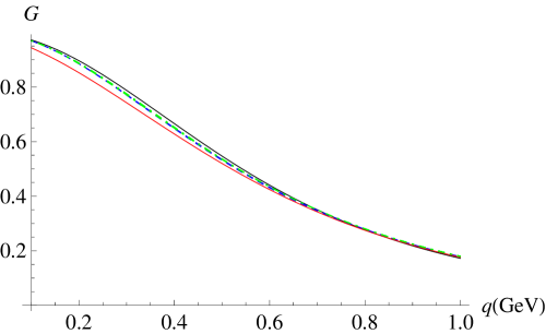
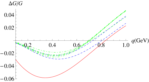
Figure 4: Top: Magnetic form factor $G_{M}(q^{2})/\mu_{p}$ of the proton: dipole parametrization and the fits. Bottom: Fractional deviation of fits from the dipole form factor $(G_{M}/\mu_{p}-G_{\rm dip})/G_{\rm dip}$. Horizontal axis: $q\;$[Gev/$c$]. The blue dashed lines are for the chain fractions, the green dot-dashed lines are for Padé approximations with $\tau=q^{2}/4m_{p}^{2}$ and the red solid one is for the Padé approximation with $q$. The dipole fit in the top graph is presented with a black solid line.

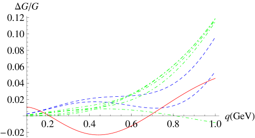
Figure 5: Fractional deviation of the magnetic form factor from the electric one $(G_{E}-G_{M}/\mu_{p})/G_{E}$ (from the same fitting procedures). Horizontal axis: $q\;$[Gev/$c$]. The blue dashed lines are for the chain fractions, the green dot-dashed lines are for Padé approximations with $\tau=q^{2}/4m_{p}^{2}$ and the red solid one is for the Padé approximation with $q$.

The low-momentum behavior of the fits is summarized in Table 3. Indeed, the fit (24) from bo1994 is excluded.

Ref.	Fit	Type	$R_{E}$	$R_{M}$	$C$
			[fm]	[fm]	[GeV-4]
as2007	(17)	Chain fraction	0.90	0.86	31.2
as2007	(18)	Chain fraction	0.90	0.87	32.2
kelly	(19)	Padé approximation ($q^{2}$)	0.86	0.85	26.8
am2007	(20)	Padé approximation ($q^{2}$)	0.88	0.86	29.2
ab2009	(21)	Padé approximation ($q^{2}$)	0.87	0.87	28.7
ab2009	(22)	Padé approximation ($q^{2}$)	0.87	0.86	28.2
va2011	(A)	Padé approximation ($q^{2}$)	0.88	0.86	29.5

Table 3: The low-momentum expansion of the fits can be expressed as $G_{E}G_{M}/\mu_{p}=1-(R_{E}^{2}+R_{M}^{2})\,q^{2}/3+Cq^{4}+...$. The values in the Table are given for central values of the fits without any uncertainty. The references are given to the papers where both electric and magnetic form factors are presented. The summary on the applied fits for the electric form factor of the proton can be found in efit . The references to the equations are given here for the magnetic form factor (see Appendix A). The related values for the standard dipole fit are $R_{E}=R_{M}=0.811\;{\rm fm}$ and $C=19.8\;{\rm GeV}^{-4}$.

VII Integration over the fits

Integrating over the fits for the optimal $q_{0}({\rm H})=0.222\;$GeV for hydrogen, we find that $I_{1>}^{\rm EM}$ varies from $-2.92\,$GeV^-1 to $-2.89\,$GeV^-1 if we exclude Padé approximation in $q$ bo1994 or from $-2.97\,$GeV^-1 if we include it. For detail see Table 4. Here, we accept

$$I_{1>}^{\rm EM}({\rm H})=-2.90(2)\;{\rm GeV}^{-1}$$

as the mean value (excluding (24)), that leads to

$$I_{1}^{\rm EM}({\rm H})-I_{1}^{R}({\rm H})=-2.82(11)\;{\rm GeV}^{-1}\;.$$

The uncertainty of integral above does not include scattering in the calculation of $I_{1>}^{\rm EM}$ because we estimated the uncertainty of this term in a more conservative way as explained above.

Fit	Type	$I_{1>}^{\rm EM}$
as2007	Chain fraction	$-2.91\;{\rm GeV}^{-1}$
as2007	Chain fraction	$-2.92\;{\rm GeV}^{-1}$
kelly	Padé approximation ($q^{2}$)	$-2.89\;{\rm GeV}^{-1}$
am2007	Padé approximation ($q^{2}$)	$-2.90\;{\rm GeV}^{-1}$
ab2009	Padé approximation ($q^{2}$)	$-2.90\;{\rm GeV}^{-1}$
ab2009	Padé approximation ($q^{2}$)	$-2.90\;{\rm GeV}^{-1}$
va2011	Padé approximation ($q^{2}$)	$-2.90\;{\rm GeV}^{-1}$
bo1994	Padé approximation ($q$)	$-2.97\;{\rm GeV}^{-1}$

Table 4: Scatter of data for $I_{1>}^{\rm EM}$ for hydrogen at ‘optimal’ $q_{0}\simeq 0.278\,\Lambda=0.234\,{\rm GeV}/c$.

Eventually, we obtain a constraint on the magnetic radius from the HFS interval in hydrogen

$$\frac{R_{E}^{2}+R_{M}^{2}}{2R_{\rm dip}^{2}}=1.025(94)\;,$$ (15)

and we remind that for the standard dipole parametrization $R_{\rm dip}^{2}=0.658\;{\rm fm}^{2}$.

The related fractional scatter is 0.013 if we exclude (24) from the consideration and it is 0.032 if we include it. The result for the combination of the proton electric and magnetic radius is consistent with the value from the standard dipole model within its 9% uncertainty.

The same evaluation can be performed for various $q_{0}$ and the results are summarized in Table 5. All the results are consistent. The scatter is below the uncertainty except for very low $q_{0}$, where behavior of the fits becomes model dependent.

$q_{0}/\Lambda$	$q_{0}$	$({R_{E}^{2}+R_{M}^{2}})/{2R_{\rm dip}^{2}}$	Scatter	Scatter∗
0.20	0.169 GeV	0.99(13)	0.03	0.10
0.25	0.211 GeV	1.02(9)	0.02	0.05
0.30	0.253 GeV	1.03(10)	0.01	0.02
0.35	0.295 GeV	1.04(11)	0.007	0.01
0.40	0.337 GeV	1.05(14)	0.004	0.007
0.50	0.421 GeV	1.08(21)	0.002	0.002

Table 5: The results for $({R_{E}^{2}+R_{M}^{2}})/{2R_{\rm dip}^{2}}$ at various $q_{0}$ for hydrogen.

Similar treatment for muonic hydrogen produces $q_{0}(\mu{\rm H})=0.263\;$GeV as the optimized value. The results of integration over the fits for $I_{1>}^{\rm EM}$ vary from $-2.77\>$GeV^-1 excluding (24) and from $-2.80\>$GeV^-1 including it to $-2.74\>$GeV^-1 (see Table 6). We consider

$$I_{1>}^{\rm EM}(\mu{\rm H})=-2.75(1)\;{\rm GeV}^{-1}$$

as the mean value that leads to

$$I_{1}^{\rm EM}(\mu{\rm H})-I_{1}^{R}(\mu{\rm H})=-2.63(13)\;{\rm GeV}^{-1}\;.$$

The uncertainty of integral above does not include scattering in a calculation of $I_{>}$ because we estimated the uncertainty of this term in a more conservative way as explained above.

Fit	Type	$I_{1>}^{\rm EM}$
as2007	Chain fraction	$-2.76\;{\rm GeV}^{-3}$
as2007	Chain fraction	$-2.77\;{\rm GeV}^{-3}$
kelly	Padé approximation ($q^{2}$)	$-2.74\;{\rm GeV}^{-3}$
am2007	Padé approximation ($q^{2}$)	$-2.75\;{\rm GeV}^{-3}$
ab2009	Padé approximation ($q^{2}$)	$-2.76\;{\rm GeV}^{-3}$
ab2009	Padé approximation ($q^{2}$)	$-2.75\;{\rm GeV}^{-3}$
va2011	Padé approximation ($q^{2}$)	$-2.75\;{\rm GeV}^{-3}$
bo1994	Padé approximation ($q$)	$-2.80\;{\rm GeV}^{-3}$

Table 6: Scatter of data for $I_{1>}^{\rm EM}$ for muonic hydrogen at ‘optimal’ $q_{0}\simeq 0.312\Lambda=0.263\,{\rm GeV}/c$.

The constraint from the HFS interval in muonic hydrogen is found to be

$$\frac{R_{E}^{2}+R_{M}^{2}}{2R_{\rm dip}^{2}}=1.13(13)\;.$$ (16)

The fractional scatter is 0.009 (excluding (24)) or 0.020 (including (24)). The result is consistent with the value from the standard dipole moment within the uncertainty of 13%.

The results obtained at various values of the separation parameter $q_{0}$ are consistent to each other (see Table 7 for details).

$q_{0}/\Lambda$	$q_{0}$	$({R_{E}^{2}+R_{M}^{2}})/{2R_{\rm dip}^{2}}$	scatter	scatter∗
0.20	0.169 GeV	1.14(19)	0.03	0.10
0.25	0.211 GeV	1.13(14)	0.02	0.05
0.30	0.253 GeV	1.13(13)	0.01	0.02
0.35	0.295 GeV	1.13(14)	0.007	0.01
0.40	0.337 GeV	1.13(16)	0.004	0.007
0.50	0.421 GeV	1.14(22)	0.002	0.002

Table 7: The results for $({R_{E}^{2}+R_{M}^{2}})/{2R_{\rm dip}^{2}}$ at various $q_{0}$ for muonic hydrogen.

VIII Conclusions

Our strategy to evaluate $I_{1}^{\rm EM}$ was dictated by our purpose, which is to determine $R_{M}$ (cf. pla ). For a different purpose the strategy would be different.

To obtain a constraint on the magnetic radius of the proton $R_{M}$, the compilation of all constraints on the electromagnetic radii of the proton is presented in Fig. 6. We plot there constraints from Fig. 1 and also present two constraints on $R_{E}^{2}+R_{M}^{2}$ derived here from a study of the HFS intervals in ordinary and muonic hydrogen.

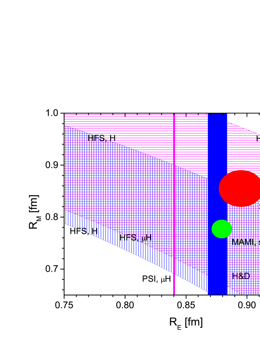
Figure 6: Determination of the rms proton charge and magnetic radii. Notation is the same as in Fig. 1. Two new striped belts are added from the HFS constraints in ordinary and muonic hydrogen above. The former is filled with vertical lines and the latter is with the horizontal ones. Their colors are the same as for the Lamb shift in the related atomic system. The squared area is the overlap of two striped areas.

That is a general picture. It already has certain features similar to those considered in paper I. The overall accuracy of spectroscopic extractions of the magnetic radius looks comparable with scattering results—not with their claimed uncertainty, but with their discrepancy.

The preliminary results on the proton magnetic radius from atomic spectroscopy are presented in Table 8. It involves all possible combinations of spectroscopic constraints on $R_{E}^{2}+R_{M}^{2}$ (from HFS) and on $R_{E}$ (from the Lamb shift). Note that ${\delta R_{M}}/{R_{M}}\approx\delta^{\prime}_{2R}$, assuming that $R_{E}$ is known with a good accuracy and that roughly $R_{E}\approx R_{M}\approx R_{\rm dip}$.

Transition/atom	Lamb ($\mu$H)	Lamb (H)
HFS (H)	0.80(8) fm	0.76(8) fm
HFS ($\mu$H)	0.88(11) fm	0.85(11) fm

Table 8: Magnetic radius of the proton from combining HFS and the Lamb shift in muonic and ordinary hydrogen.

If we accept the value of the proton charge radius as

$$R_{E}=0.86(2)\;{\rm fm}\;,$$

which seems a reasonable choice until the controversy in its determination is not resolved, then we arrive at

$$R_{M}=0.78(8)\;{\rm fm}\;,$$

as to the best constraint on the magnetic radius from spectroscopy.

We have performed a number of consistency checks described above such as consideration of various values of the separation parameter. All the results are consistent. The estimation of the $q^{4}$ term is consistent with all fits with reasonable behavior at low $q$ discussed in Appendix (as well as with the fits from MAMI (see thesis for detail)). In case of the fits considered above the only fit with unreasonable behavior is that from bo1994 , which in particular produces infinite values of the charge and mangetic radii. It is important that all fits but (24) agree with each other within at 1% level in the region where the separation parameter was chosen in Tables 5 and 7 as seen in Fig. 7.

The fit of bo1994 with incorrect behavior at low momentum transfer is responsible for a scatter of values of $G_{M}(q_{0})$ bigger than $\pm 1\%$ (see Fig. 7) (cf. efit ). However, taking into account its unrealistic behavior, that is acceptable. The other fits agree with each other within 1% in the region crucial for a choice of $q_{0}$. A similar situation with the electric radius (see Fig. 6 of paper I).

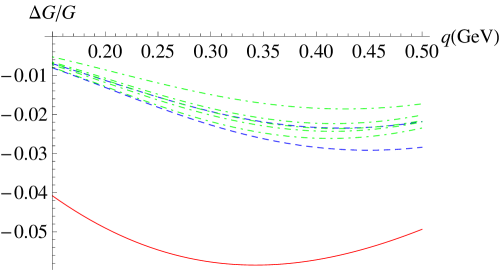
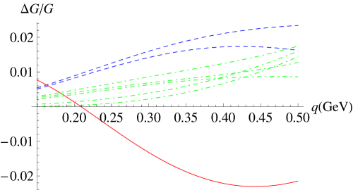
Figure 7: Top: Fractional deviation of the magnetic form factor from the dipole form factor $(G_{M}/\mu_{p}-G_{\rm dip})/G_{\rm dip}$. Bottom: Fractional deviation of the magnetic form factor from the electric one $(G_{E}-G_{M}(q^{2})/\mu_{p})/G_{E}$. Horizontal axis: $q\;$[Gev/$c$] and the range $0.2-0.5\;{\rm GeV}/c$ is crucial for $q_{0}$ in all three cases considered.

A value of the magnetic radius extracted from electron-proton scattering strongly depends on treatment of the proton polarizability comm ; resp . To apply the Rosenbluth separation, one has to rely on a certain model for the proton polarizability. We note, however, that the electric form factor $G_{E}$ at low momentum transfer is less sensitive to the model and as far as we are not going to go too low, one may use experimental results on $G_{M}/G_{E}$ from recoil polarimetry (see, e.g., zhan ), which are free of the polarizability problem.

Similarly to the case of examination for $R_{E}$ in efit , we conclude that the estimation of the uncertainty of the form factors at the level of 1% for applied $q_{0}$ is validated by the behavior of the fits and by the scale of the scatter. Nevertheless, a direct investigation of the problem would be useful.

The author is grateful to S. Eidelman and V. Ivanov for useful discussions. This work was supported in part by DFG under grant HA 1457/9-1.

Appendix A Fits for $G_{M}$ applied in the paper

The fits for $G_{M}$ applied in the papers fall into three classes.

1). Two fits deal with chain fractions. Those are from from Arrington and Sick, 2007, as2007 . One is from analysis of as2007 alone

$$\frac{G_{M}(Q^{2})}{\mu_{p}} = \frac{1}{1+\frac{3.173Q^{2}}{1-\frac{0.314Q^{2}}{1-\frac{1.165Q^{2}}{1+5.619\frac{Q^{2}}{1-1.087Q^{2}}}}}}\;,$$ (17)

while the other exploit the evaluation of the two-photon effects from bm2005

$$\frac{G_{M}(q^{2})}{\mu_{p}} = \frac{1}{1+\frac{3.224Q^{2}}{1-\frac{0.313Q^{2}}{1-\frac{0.868Q^{2}}{1+\frac{4.278Q^{2}}{1-1.102Q^{2}}}}}}\;,$$ (18)

and

Five fits are Padé approximations with polynomials in $q^{2}$. Those include fits from Kelly, 2004, kelly

$$\frac{G_{M}(q^{2})}{\mu_{p}} = \frac{1+0.12\tau}{1+10.97\tau+18.86\tau^{2}+6.55\tau^{3}}\;,$$ (19)

where

$$\tau=q^{2}/4m_{p}^{2}\;,$$

from Arrington et al., 2007, am2007

$$\frac{G_{M}(q^{2})}{\mu_{p}} = \frac{1-1.465\tau+1.260\tau^{2}+0.262\tau^{3}}{1+9.627\tau+11.179\tau^{4}+13.245\tau^{5}}\;,$$ (20)

from Alberico et al., 2009, ab2009

$$\frac{G_{M}(q^{2})}{\mu_{p}} = \frac{1+1.53\tau}{1+12.87\tau+29.16\tau^{2}+41.40\tau^{3}}$$ (21)

$$\frac{G_{M}(q^{2})}{\mu_{p}} = \frac{1+1.09\tau}{1+12.31\tau+25.57\tau^{2}+30.61\tau^{3}}\;,$$ (22)

and two fits Venkat et al., 2011, va2011

$$\frac{G_{M}(q^{2})}{\mu_{p}} = \frac{1-1.43573\tau+1.19052066\tau^{2}+0.25455841\tau^{3}}{D_{V}}\;,$$

$$D_{V} = 1+9.70703681\tau+3.7357\times 10^{-4}\tau^{2}$$ (23)

$$+6.0\times 10^{-8}\tau^{3}+9.9527277\tau^{4}$$

$$+12.7977739\tau^{5}\;.$$

The remaining fit from Bosted, 1995, bo1994

$$\frac{G_{M}(q^{2})}{\mu_{p}} = \left(1+0.35Q+2.44Q^{2}+0.50Q^{3}\right.$$ (24)

$$+\left.1.04Q^{4}+0.34Q^{5}\right)^{-1}$$

is a Padé approximation with polynomials in $q$. That is a phenomenological fit designed to be used for medium and high $q$. It is not expected to be appropriate at low $q$. Providing a reasonably good approximation at medium momentum transfer, the fit apparently has incorrect low-$q$ behavior and incorrect analytic properties such as a branch point at $q^{2}=0$.

References

• (1) S.G. Karshenboim, eprint arXiv:1405.6039.
• (2) I. Sick, Phys. Lett. B 576, 62 (2003); Can. J. Phys. 85, 409 (2007).
• (3) J.C. Bernauer, P. Achenbach, C. Ayerbe Gayoso, R. Bรถhm, D. Bosnar, L. Debenjak, M.O. Distler, L. Doria, A. Esser, H. Fonvieille, J.M. Friedrich, J. Friedrich, M. Gรณmez Rodrรญguez de la Paz, M. Makek, H. Merkel, D.G. Middleton, U. Mรผller, L. Nungesser, J. Pochodzalla, M. Potokar, S. Sรกnchez Majos, B.S. Schlimme, S. ล irca, Th. Walcher, and M. Weinriefer, Phys. Rev. Lett. 105, 242001 (2010).
• (4) X. Zhan, K. Allada, D.S. Armstrong, et al., Phys. Lett. B 705, 59 (2011).
• (5) S.G.ย Karshenboim, Annalen der Physik 525, 472 (2013).
• (6) S.G.ย Karshenboim, Physics-Uspekhi 56, 883 (2013).
• (7) P.J. Mohr, B.N. Taylor, and D.B. Newell, Rev. Mod. Phys. 84, 1527 (2012).
• (8) R. Pohl, A. Antognini, F. Nez, F.D. Amaro, F. Biraben, J.M.R. Cardoso, D.S. Covita, A. Dax, S. Dhawan, L.M.P. Fernandes, A. Giesen, T. Graf, T.W. Hรคnsch, P. Indelicato, L. Julien, Cheng-Yang Kao, P. Knowles, E.-O. Le Bigot, Yi-Wei Liu, J.A.M. Lopes, L. Ludhova, C.M.B. Monteiro, F. Mulhauser, T. Nebel, P. Rabinowitz, J.M.F. dos Santos, L.A. Schaller, K. Schuhmann, C. Schwob, D. Taqqu, J.F.C.A. Veloso and F. Kottmann, Nature (London) 466, 213 (2010).
• (9) A.ย Antognini, F. Nez, K. Schuhmann, F.D. Amaro, F. Biraben, J.M.R. Cardoso, D.S. Covita, A. Dax, S. Dhawan, M. Diepold, L.M.P. Fernandes, A. Giesen, A.L. Gouvea, T. Graf, T.W. Hรคnsch, P. Indelicato, L. Julien, Cheng-Yang Kao, P. Knowles, F. Kottmann, E.-O. Le Bigot, Yi-Wei Liu, J.A.M. Lopes, L. Ludhova, C.M.B. Monteiro, F. Mulhauser, T. Nebel, P. Rabinowitz, J.M.F. dos Santos, L.A. Schaller, C. Schwob, D. Taqqu, J.F.C. A. Veloso, J. Vogelsang, R. Pohl, Science, 339 417 (2013).
• (10) J. Arrington, Phys. Rev. Lett. 107, 119101 (2011).
• (11) J.C. Bernauer, P. Achenbach, C. Ayerbe Gayoso, R. Bรถhm, D. Bosnar, L. Debenjak, M.O. Distler, L. Doria, A. Esser, H. Fonvieille, J.M. Friedrich, J. Friedrich, M. Gรณmez Rodrรญguez de la Paz, M. Makek, H. Merkel, D.G. Middleton, U. Mรผller, L. Nungesser, J.Pochodzalla, M.Potokar, S. Sรกnchez Majos, B.S. Schlimme, S. ล irca, Th. Walcher, and M. Weinriefer, Phys. Rev. Lett. 107, 119102 (2011).
• (12) S.G.ย Karshenboim, Phys.ย Rep.ย  422, 1 (2005).
• (13) S.G.ย Karshenboim, Can. J. Phys. 78, 639 (2000).
• (14) N.E.ย Rothery and E.A.ย Hessels, Phys. Rev. A 61, 044501 (2000);
N.ย Kolachevsky, M.ย Fischer, S.G.ย Karshenboim, and T.W.ย Hรคnsch, Phys. Rev. Lett. 92, 033003 (2004);
N. Kolachevsky, A. Matveev, J. Alnis, C.G. Parthey, S.G. Karshenboim, and T. W. Hรคnsch, Phys. Rev. Lett. 102, 213002 (2009).
• (15) S.G.ย Karshenboim, Phys. Lett. A225, 97 (1997).
• (16) A.V. Volotka, V.M. Shabaev, G. Plunien, and G. Soff, Eur. Phys. J. D 33, 23 (2005).
• (17) A. Dupays, A. Beswick, B. Lepetit, C. Rizzo, and D. Bakalov, Phys. Rev. A 68, 052503 (2003).
• (18) J. Arrington and I. Sick, Phys. Rev. C76, 035201 (2007).
• (19) J.J. Kelly, Phys. Rev. C 70, 068202 (2004).
• (20) J. Arrington, W. Melnitchouk, and J.A. Tjon, Phys. Rev. C76, 035205 (2007).
• (21) W.M. Alberico, S.M. Bilenky, C. Guinti, and K.M. Graczyk, Phys. Rev. C79, 065204 (2009).
• (22) S. Venkat, J. Arrington, G. A. Miller and X. Zhan, Phys. Rev. C83, 015203 (2011).
• (23) P.E. Bosted, Phys. Rev. C51, 409 (1995).
• (24) J. Bernauer, Measurement of the elastic electron-proton cross section and separation of the electric and magnetic form factor in the $Q^{2}$ range from 0.004 to 1$({\rm GeV}/c)^{2}$. Ph.D. Thesis, Mainz, 2010. Available at http://wwwa1.kph.uni-mainz.de/A1/publications/doctor/bernauer.pdf.
• (25) P.G. Blunden, W. Melnitchouk, and J.A. Tjon, Phys. Rev. C72, 034612 (2005).