On adaptive timestepping for weakly instationary solutions of hyperbolic conservation laws via adjoint error control

Abstract.

We study a recent timestep adaptation technique for hyperbolic conservation laws. The key tool is a space-time splitting of adjoint error representations for target functionals due to Süli[19] and Hartmann[13]. It provides an efficient choice of timesteps for implicit computations of weakly instationary flows. The timestep will be very large in regions of stationary flow, and become small when a perturbation enters the flow field. Besides using adjoint techniques which are already well-established, we also add a new ingredient which simplifies the computation of the dual problem. Due to Galerkin orthogonality, the dual solution $\varphi$ does not enter the error representation as such. Instead, the relevant term is the difference of the dual solution and its projection to the finite element space, $\varphi-\varphi_{h}$. We can show that it is therefore sufficient to compute the spatial gradient of the dual solution, $w=\nabla\varphi$. This gradient satisfies a conservation law instead of a transport equation, and it can therefore be computed with the same algorithm as the forward problem, and in the same finite element space. We demonstrate the capabilities of the approach for a weakly instationary test problem for scalar conservation laws.

1. Introduction

For explicit calculations of instationary solutions to hyperbolic conservation laws, the timestep is dictated by the CFL condition due to Courant, Friedrichs and Lewy [4], which requires that the numerical speed of propagation should be at least as large as the physical one. For implicit schemes, the CFL condition does not provide a restriction, since the numerical speed of propagation is infinite. Depending on the equations and the scheme, restrictions may come in via the stiffness of the resulting nonlinear problem. These restrictions are usually not as strict as in the explicit case, where the CFL number should be below unity. For implicit calculations, CFL numbers of 10, 100 or even 1000 may well be possible. Therefore, it is a serious question how large the timestep, i.e. the CFL number, should be chosen.

We are particularly interested in timestep control which is based upon computable, a-posteriori error estimates. In [17, 18] Kröner and Ohlberger based their space-time adaptivity upon $L^{1}$, Kuznetsov type estimates for scalar conservation laws. In [8, 9, 10, 11, 12], Eriksson and Johnson developed space-time adaptive methods for parabolic pde’s. These a-posteriori error estimates require the solution of an adjoint problem. A space-time projection of the adjoint solution makes it possible to consider spatial and temporal error separately. They closed the error estimates by an a-priori bound on the dual solution. In [19, 20], Süli and Houston developed an analogous approach for hyperbolic transport equations.

The work of Eriksson and Johnson has been extended by many authors, see, for example, the review articles of Becker and Rannacher [5, 6] and of Hoffman and Johnson [16]. We would like to mention that we learned a lot about these developments from the unpublished thesis of Ralf Hartmann [13]. Instead of relying upon an (usually pessimistic) a-priori error estimate for the adjoint solution, Hartmann and others [14, 20] computed the adjoint solution and hence obtained an (in principle exact) error representation.

More recently these methods have also been developed for hyperbolic problem by Barth, Hartmann, Houston, Giles, Süli, Schwab and others. An excellent collection of review papers may be found in [1].

Let us briefly summarize the space-time splitting of the adjoint error representation (see [8, 9, 10, 11, 12, 5, 19, 13] for details). The error representation expresses the error in a target functional as a scalar product of the finite element residual with the dual solution. This error representation is decomposed into separate spatial and temporal components. The spatial part will decrease under refinement of the spatial grid, and the temporal part under refinement of the timestep. Technically, this decomposition is achieved by inserting an additional projection. Usually, in the error representation, one subtracts from the dual solution its projection onto space-time polynomials. Now, we also insert the projection of the dual solution onto polynomials in time having values which are $H^{1}$ functions with respect to space.

This splitting can be used to develop a strategy for a local choice of timestep. Here we add to the results in [19, 13] by studying a weakly instationary solution to Burgers’ equation, for which the timestep will be very large (and we will quantify this) in regions of stationary flow, and become small when a perturbation enters the flow field. We believe that this type of flow is a prime example where the space-time splitting can become useful.

Besides applying adjoint techniques which are already well-established to a new test problem, we also add a new ingredient which simplifies and accelerates the computation of the dual problem. Due to Galerkin orthogonality, the dual solution $\varphi$ does not enter the error representation as such. Instead, the relevant term is the difference of the dual solution and its projection to the finite element space, $\varphi-\varphi_{h}$. We can show that it is therefore sufficient to compute the spatial gradient of the dual solution, $w=\nabla\varphi$. This gradient satisfies a conservation law instead of a transport equation, and it can therefore be computed with the same algorithm as the forward problem, and in the same finite element space.

Our goal here is time step adaptation. Ultimately, this will become a building block of an aerodynamic and aeroelastic solver which is currently being developed by the SFB 401 research group at RWTH Aachen [3]. In that solver, multiscale analysis is used to compress data, coarsen and refine the spatial grid. Time stepping for instationary problems is done by a methods of lines approach, using explicit or implicit Runge-Kutta schemes. The latter is, of course, a standard set-up used for aerodynamic, or conservation law, solvers.

In the aerodynamical applications which we have in mind, we may have to resolve many different features of the flow, more than can be controlled by a small number of functionals like drag and lift. Therefore, an adaptive monitoring of the complete flow field, as done by the multiscale analysis, is very desirable.

Here we develop our strategy for a test case. Since we focus on timestep adaptation we will use uniformly refined meshes in space. Starting with a very coarse spatial mesh and CFL below unity, we gradually establish sequences of timesteps which are well adapted to the physical problem at hand. The scheme detects stationary regions, where it switches to very high CFL numbers, but reduces the time steps appropriately as soon as a perturbation enters the flow field.

Depending on the CFL number and the cost of the nonlinear solver, the adaptive scheme chooses either explicit or implicit timesteps. For reasons of efficiency, very small timesteps $C\!F\!L\ll 1$ may be merged into a single step. This strategy is detailed in Section 4.1.

Once we arrive at the fine spatial mesh, on which we really want to compute and where most of the work is being done, we already work with a very efficient time step. Moreover, we have a rational criterion what the finest grid should be.

The paper is organized as follows: in Section 2 we review the theoretical background for our adaptive timestep control: DG and FV methods, control of target functionals, error representation, space-time splitting, error estimates. The new conservative approach for solving the dual problem is presented in Section 3. In Section 4 we define our adaptive strategy and apply it to compute perturbations of a stationary shock. Some conclusions are drawn in Section 5.

2. Derivation of space-time-split error estimates

In this section, we recall some of the theoretical background of adjoint error control, and we represent the extensions needed in our time adaptive strategy. In Section 2.1 we introduce the DG method used in the paper. In Section 2.2 we state the adjoint based error representation for target functionals. In Section 2.3 we introduce a variant of the projections in space and time which lead to a splitting of the error representation. One part decreases when the spatial grid is refined, and the other part decays with the timestep. The corresponding decay rates are a crucial ingredient of the time-adaptation strategy. This strategy and its application will be presented in Section 4 below.

2.1. Discontinuous Galerkin methods for conservation laws

Let $D$ be an open connected subset of $\mathbb{R}^{d}$, $d\geq 1$, let $I:=(0,T)$ be the time interval and let $\Omega:=D\times I$ be the space-time domain, with boundary $\Gamma$ and outside unit normal $\nu$. We consider the system

(1) $$\partial_{t}u+\nabla f(u) =0\quad\mbox{in }\Omega,$$

(2) $$\quad f_{\nu}(u) =\gamma_{\nu}\quad\mbox{on }\Gamma_{in},$$

where $u=(u_{1},\ldots,u_{m})^{T}:\Omega\rightarrow\mathbb{R}^{d}$ is the vector of conservative variables and $f(u)=(f_{1}(u),\dots,f_{d}(u))$ the flux matrix, with $f_{i}\in C^{1}(\mathbb{R}^{m},\mathbb{R}^{m})$. The vector

$$f_{\nu}(u):=(f(u),u)\cdot\nu$$

is the space-time normal flux across the boundary, and for scalar equations, the inflow boundary is given by

$$\Gamma_{in}:=\{(x,t)\in\Gamma\mid\frac{d}{du}((f(u),u)\cdot\nu<0\}.$$

Note that (2) includes initial data, since $D\times\{0\}\subset\Gamma_{in}$, and $f_{\nu}(u(x,0))=u(x,0)$. For systems of conservation laws, the definition of in- and outflow boundaries may be generalized via characteristic decompositions [15, 20].

Let us define a partition of our time interval $I$ into subintervalls $I_{n}=(t_{n-1},t_{n})$, where

$$0=t_{0}<t_{1}<\ldots<t_{n}<\ldots<t_{N}=T.$$

Later on this partition will be defined automatically by the adaptive algorithm. Furthermore we define a regular polygonal spatial grid $\mathcal{T}_{D}=\bigcup_{j}\{D_{j}\}$ such that $\overline{D}=\bigcup_{j}\overline{D_{j}}$. We denote the corresponding space time prisms by

$$\Omega_{j}^{n}:=D_{j}\times I_{n}.$$

For future reference, we denote the outward unit normal vector to $\Omega_{j}^{n}$ by $\nu_{j}^{n}$ or simply $\nu$. Thus we have constructed a subdivision

$$\mathcal{T}_{\Omega}=\bigcup_{j,n}\{\Omega_{j}^{n}\}$$

of the computational domain $\Omega$. The spatial discretisation $\mathcal{T}_{D}$ can change adaptively from timestep to timestep, and for each fixed time interval $I_{n}$, the timestep is global (i.e. it is the same for all spatial cells $D_{j}$).

Remark 1.

We do not admit local timesteps, since we want to couple our time-adaptive strategy to standard Runge-Kutta Finite Volume methods and Runge-Kutta Discontinuous Galerkin methods.

On this grid we define the following function spaces: First, let $S_{h}(\Omega)$ be the mesh dependent broken space of discontinuous piecewise $H^{1}$ functions defined on $\mathcal{T}_{\Omega}$,

(3) $$S_{h}(\Omega):=\left\{u\mid u_{\mid_{\Omega_{j}^{n}}}\in H^{1}(\Omega_{j}^{n}),\forall\Omega_{j}^{n}\in\mathcal{T}_{\Omega}\right\}.$$

Furthermore we denote by $S_{h}^{s,r}(\Omega)$ the (locally) finite dimensional space consisting of discontinuous piecewise polynomial functions of degree $s$ in space and $r$ in time defined on $\mathcal{T}_{h}$

(4) $$S_{h}^{s,r}(\Omega):=\left\{u_{h}\mid u_{h}(\cdot,t)\in P_{s}(D_{j}),\forall t\in{I_{n}},u_{h}(x,\cdot)\in P_{r}(I_{n}),\forall x\in{D_{j}},\forall D_{j}\times I_{n}\in\mathcal{T}_{\Omega}\right\},$$

where $P_{r}(I_{n})$ denotes the space of polynomials of degree $r$ on $I_{n}$ and $P_{s}(D_{j})$ the space of polynomials of degree $s$ on $D_{j}$. Given a cell $\Omega_{j}^{n}$ and a point $(x,t)\in\Gamma_{j}^{n}$, we define the inner ($u^{+}$) and outer ($u^{-}$) values of a function $u\in S_{h}(\Omega)$ with via

(5) $$u^{\pm}(x,t):=\lim_{{\delta\searrow 0+}\atop{\delta\nearrow 0-}}u((x,t)-\delta\nu_{j}^{n}).$$

Defining the DG method for nonlinear conservation laws, whose solutions in general contain shock waves, requires a careful application of the theory of weak solutions, which states that for a weak solution $u$ and a continuously differentiable test functions $v$,

$$-(u,\partial_{t}v)_{\Omega_{j}^{n}}-(f(u),\nabla v)_{\Omega_{j}^{n}}+(f_{\nu}(u),v)_{\Gamma_{j}^{n}}=0\quad\forall j,n.$$

Thus we have to define the normal flux $f_{\nu}(u)$ at the cell boundaries, where the approximate solution $u_{h}$ is discontinuous. This can be done with the help of numerical flux functions, which we denote by $f_{\nu}^{\ast}$. So suppose that $(x,t)\in\Gamma_{j}^{n}\setminus\Gamma$ is contained in an interior edge. If $(x,t)\in\partial D_{j}\times I_{n}$, so that the normal points into the spatial direction, then the canonical choice for $f_{\nu}^{\ast}$ is an approximate Riemann solver

(6) $$f_{\nu}^{\ast}:=f(u_{h}^{+},u_{h}^{-},n_{j}),$$

where $n_{j}$ is the outer normal to $D_{j}$ (i.e. $\nu_{j}^{n}=(n_{j},0)$). We require that the flux $f_{\nu}^{\ast}$ is consistent and conservative in the sense of Lax. If, on the other hand, $(x,t)\in D_{j}\times\partial I_{n}$, so that the normal points into the time direction and $f_{\nu}(u)=u$, then we simply require that $f_{\nu}^{\ast}$ be a convex combination of $u_{h}(x,t^{\pm})$. More specifically, suppose that $t=t_{n}$. Then we set

(7) $$f_{\nu}^{\ast}:=u_{h}^{\ast}(x,t_{n}):=(1-\theta)u_{h}(x,t_{n}^{+})+\theta u_{h}(x,t_{n}^{-})$$

for some value $\theta\in[0,1]$. Different values of $\theta$ will yield different time discretisations, e.g. explicit Euler for $\theta=0$, implicit Euler for $\theta=1$, if we work with piecewise constant ansatz functions.

On the boundary of the domain, i.e. for $(x,t)\in\Gamma$, we set

(10) $$f_{\nu}^{\ast}:=\left\{\begin{array}[]{ll}\gamma_{\nu}&\mathrm{if}\;(x,t)\in\Gamma_{in}\\ f_{\nu}(u^{+}_{h}(x,t))&\mathrm{if}\;(x,t)\in\Gamma_{out}\end{array}\right.$$

In the following definition we simply state the resulting DG(s,r) method, which is a discontinuous method both in space and time. This definition is very similar to, see e.g. [2, 7, 14, 20] and the references therein.

Definition 2.

(i) The abstract semilinear form $\mathcal{N}:S_{h}(\Omega)\times S_{h}(\Omega)\to\mathbb{R}$ is given by

(11) $$\mathcal{N}\left(u_{h},v_{h}\right):=\sum_{j,n}\left\{(\partial_{t}u_{h}+\nabla f(u_{h}),v_{h})_{\Omega_{j}^{n}}+(f_{\nu}^{\ast}-f_{\nu}(u_{h}^{+}),v_{h}^{+})_{\partial\Omega_{j}^{n}}\right\}.$$

(ii) Now the DG(s,r) finite element method for the system of hyperbolic conservation laws (2) is defined as follows: Find $u_{h}\in S_{h}^{s,r}(\Omega)$, such that

(12) $$\mathcal{N}\left(u_{h},v_{h}\right)=0\quad\forall v_{h}\in S_{h}^{s,r}(\Omega).$$

As usual, the variational formulation (11), (12) can be exploited as follows: Given $u_{h}\in S_{h}(\Omega)$, $\mathcal{N}(u_{h},\cdot)$ is a linear functional on $S_{h}(\Omega)$. Thus it can be represented by an element of $S_{h}(\Omega)$, which we call $R(u_{h})$, the residual. On the interior of a cell $\Omega_{j}^{n}$ we introduce the cell residual

(13) $$R_{h}:=\partial_{t}u_{h}+\nabla f(u_{h})$$

and on the boundaries $\Gamma_{j}^{n}$ the edge residual

(14) $$r_{h}:=f_{\nu}^{\ast}-f_{\nu}(u_{h}^{+}).$$

Then (11) can be rewritten as

(15) $$(R(u_{h}),v_{h})=\sum_{j,n}\left\{(R_{h},v_{h})_{\Omega_{j}^{n}}+(r_{h},v_{h}^{+})_{\partial\Omega_{j}^{n}}\right\}.$$

The $DG(s,r)$ solution $u_{h}\in S_{h}^{s,r}(\Omega)$ of (12) is now given by

(16) $$(R(u_{h}),v_{h})=0\quad\forall v_{h}\in S_{h}^{s,r}(\Omega),$$

which is the classical Galerkin orthogonality: the residual $R(u_{h})$ is orthogonal to the test space $S_{h}^{s,r}(\Omega)$.

In the following, we mostly work with the $DG(0,0)$ and $DG(1,1)$ methods, both in their explicit ($\theta=0$) and implicit ($\theta=1$) form. The DG(0,0) method is equivalent to a first order accurate finite volume scheme, using explicit order implicit Euler scheme for the time integration. In [2], Barth and Larson derive a weak formulation of the form (16) for higher oder accurate finite volume schemes.

Therefore, the techniques presented in this paper can be applied to finite volume and Discontinuous Galerkin methods.

2.2. Adjoint error representation for target functional

In this section we define the class of target functionals treated in this paper, state the corresponding adjoint problem and recall the classical error representation which we will later use for adaptive time step control.

Our objective is to estimate the error in a user specified functional $J(u)$, which can be expressed as a sum of weighted integrals over the domain $\Omega$ and the outflow boundary $\Gamma_{out}$. Typical examples of such functionals are the lift or the drag of a body immersed into a fluid.

To simplify matters we consinder functionals of the following form:

$$J(u)=(u,\psi)_{\Omega}-(f_{\nu}(u),\psi_{\Gamma})_{\Gamma_{out}}$$

Our purpose is to control the error

$$J(u)-J(u_{h}).$$

In order to derive the classical error representation one linearizes the evolution equation satisfied by the error $u-u_{h}$ and works with the adjoint equation of the linearized error equation. Thus we introduce an approximate Jacobian $\overline{a}(u;u_{h})$ of $f$ by

(17) $$\overline{a}(u;u_{h}) :=\int\limits_{0}^{1}\frac{d}{d\tau}f(u_{h}+\tau(u-u_{h}))d\tau.$$

Note that

$$f(u)-f(u_{h}) =\overline{a}(u;u_{h})(u-u_{h}).$$

In practice we linearize around the approximate solution. A direct calculation yields the following theorem:

Theorem 3.

Suppose $\varphi\in H^{1}(\Omega)$ solves the adjoint problem

(18) $$\varphi =\psi_{\Gamma}\quad\mathrm{on}\;\Gamma_{out}$$

(19) $$\partial_{t}\varphi+\overline{a}(u;u_{h})\nabla\varphi =\psi\quad\;\;\mathrm{in}\;\Omega.$$

Then for all $\varphi_{h}\in S_{h}^{s,r}(\Omega)$, the error in the target functional satisfies

(20) $$J(u)-J(u_{h})=(R(u_{h}),\varphi-\varphi_{h}).$$

Equivalently one can also define the adjoint solution via a variational formulation (see e.g. [2, 14, 20]). In [21] Tadmor proves the well-posedness of the adjoint problem (18) – (19) for scalar, convex, one-dimensional conservation laws. The key observation is that, if the forward solution $u$ has jump discontinuities, then due to the entropy condition the jump of the transport coefficient $\overline{a}(u;u_{h})$ has a distinct sign. This makes it possible to follow the characteristics of the adjoint problem backwards in time.

Identity (20) is the error representation which we discussed in the introduction and onto which we are going to base our adaptive strategy. By definition (13) - (15) of the residual $R(u_{h})$, the error representation may be decomposed as a sum over the cells and edges of inner products of the local residuals with the solution of our dual problem. Due to Galerkin orthogonality (16), we can subtract an arbitrary test function $\varphi_{h}$, which is very convenient when we derive local error estimates later on.

2.3. Space-time splitting and the error estimate

The error representation (20) is not yet suitable for time adaptivity, since it combines space and time components of the residual and of the difference $\varphi-\varphi_{h}$ of the dual solution and the test function. The main result of this section is an error estimate whose components depend either on the spatial grid size $h$ or the time step $k$, but never on both. The key ingredient is a space-time splitting of (20) based on $L^{2}$ projections. Similar space-time projections were introduced previously in [13, 19]. Here we adapt them to the finite element spaces used in the error representation (20).

Let $P_{s,r}(\Omega_{j}^{n})=P_{s}(D_{j})\times P_{r}(I_{n})$ be the space of polynomials of degree $s$ on ${D_{j}}$ and $r$ on $I_{n}$. Furthermore let $\hat{P}_{I_{n}}^{r}(\Omega_{j}^{n})=\{w\in L^{2}(\Omega_{j}^{n})|w(x,\cdot)\in P_{r}(I_{n}),\forall x\in D_{j}\}$, and $\hat{P}_{D_{j}}^{s}=\{w\in L^{2}(\Omega_{j}^{n})|w(\cdot,t)\in P_{s}(D_{j}),\forall t\in I_{n}\}$. For $r\geq 0$ define the $L^{2}$ projection $\Pi_{I_{n}}^{r}:L^{2}(\Omega_{j}^{n})\to\hat{P}_{I_{n}}^{r}(\Omega_{j}^{n})$ via

(21) $$(u-\Pi_{I_{n}}^{r}u,\varphi)_{I_{n}}=0\quad\forall\varphi\in\hat{P}_{I_{n}}^{r}(\Omega_{j}^{n}),\forall x\in D_{j},$$

and for $s\geq 0$ define the $L^{2}$ projection $\Pi_{D_{j}}^{s}:L^{2}(\Omega_{j}^{n})\to\hat{P}_{D_{j}}^{s}(\Omega_{j}^{n})$ via

(22) $$(u-\Pi_{D_{j}}^{s}u,\varphi)_{D_{j}}=0\quad\forall\varphi\in\hat{P}_{D_{j}}^{s}(\Omega_{j}^{n}),\forall t\in I_{n}.$$

Similarly let the $L^{2}$ projection $\Pi_{\Omega_{j}^{n}}^{s,r}:=L^{2}(\Omega_{j}^{n})\to P_{s,r}(\Omega_{j}^{n})$ be defined via

(23) $$(u-\Pi_{\Omega_{j}^{n}}^{s,r}u,\varphi)_{\Omega_{j}^{n}}=0\quad\forall\varphi\in P_{s,r}(\Omega_{j}^{n}).$$

Note that $\Pi_{\Omega_{j}^{n}}^{s,r}=\Pi_{{D_{j}}}^{s}\Pi_{I_{n}}^{r}$.

First we choose $\varphi_{h}$ in the error representation (20) to be $\varphi_{h}=\Pi_{h,k}^{s,r}\varphi$, i.e. $\varphi_{h}\mid_{\Omega_{j}^{n}}=\Pi_{{D_{j}}}^{s}\Pi_{I_{n}}^{r}\varphi=\Pi_{I_{n}}^{r}\Pi_{{D_{j}}}^{s}\varphi$, with $\Pi_{I_{n}}^{r}$ and $\Pi_{{D_{j}}}^{s}$ as defined above. Using the identity

$$\varphi-\Pi_{h,k}^{s,r}\varphi=\varphi-\Pi_{I_{n}}^{r}\varphi+\Pi_{I_{n}}^{r}\varphi-\Pi_{h,k}^{s,r}\varphi=(id-\Pi_{I_{n}}^{r})\varphi+(id-\Pi_{D_{j}}^{s})\Pi_{I_{n}}^{r}\varphi$$

we obtain the following splitting of the error representation:

(24) $$J(u)-J(u_{h}) =(R(u_{h}),(id-\Pi_{I_{n}}^{r})\varphi+(id-\Pi_{D_{j}}^{s})\Pi_{I_{n}}^{r}\varphi)$$

(25) $$=\sum_{j,n}\{\underbrace{(R_{h},(id-\Pi_{I_{n}}^{r})\varphi)_{\Omega_{j}^{n}}+(r_{h},(id-\Pi_{I_{n}}^{r})\varphi^{+})_{\partial\Omega_{j}^{n}}}_{\eta_{k}^{jn}}$$

(26) $$\phantom{=\sum_{j,n}}+\underbrace{(R_{h},(id-\Pi_{D_{j}}^{s})\Pi_{I_{n}}^{r}\varphi)_{\Omega_{j}^{n}}+(r_{h},(id-\Pi_{D_{j}}^{s})\Pi_{I_{n}}^{r}\varphi^{+})_{\partial\Omega_{j}^{n}}}_{\eta_{h}^{jn}}\}$$

(27) $$=:\eta_{k}+\eta_{h},$$

where $\eta_{k}$ is the time-component and $\eta_{h}$ the space-component of the error representation $\eta$.

In this paper we consider grids, which are locally tensor products of a spatial grid $\mathcal{T}_{D_{j}}$ and a timestep $I_{n}$. For an implicit Runge-Kutta Finite Volume Method $\eta_{k}^{jn}$ and $\eta_{h}^{jn}$ then take the form

$$\eta_{k}^{jn}= (R_{h},(id-\Pi_{I_{n}}^{r})\varphi)_{D_{j}\times I_{n}}+(f_{\nu}^{\ast}-f_{\nu}(u_{h}^{+}),(id-\Pi_{I_{n}}^{r})\varphi^{+})_{\partial D_{j}\times I_{n}}$$

$$+(\left[u_{h}\right]_{n-1},(id-\Pi_{I_{n}}^{r})\varphi_{n-1}^{+})_{D_{j}}$$

$$\eta_{h}^{jn}= (R_{h},(id-\Pi_{D_{j}}^{s})\Pi_{I_{n}}^{r}\varphi)_{D_{j}\times I_{n}}+(f_{\nu}^{\ast}-f_{\nu}(u_{h}^{+}),((id-\Pi_{D_{j}}^{s})\Pi_{I_{n}}^{r}\varphi)^{+})_{\partial D_{j}\times I_{n}}$$

$$+(\left[u_{h}\right]_{n-1},((id-\Pi_{D_{j}}^{s})\Pi_{I_{n}}^{r}\varphi)_{n-1}^{+})_{D_{j}}$$

where the flux difference on the spatial boundaries $\partial D_{j}\times I_{n}$ and the jump of $u_{h}$ on the time boundary $D_{j}\times\{t_{n-1}\}$ are realizations of the residual term $r_{h}$ in (14).

For future reference, we also introduce the quantities

(28) $$\eta_{k} :=\sum_{j,n}\eta_{k}^{jn} \eta_{h} :=\sum_{j,n}\eta_{h}^{jn}$$

(29) $$\bar{\eta}_{k}^{n} :=\frac{1}{k_{n}}\sum_{{D_{j}}\in\mathcal{T}}|\bar{\eta}_{k}^{jn}| \bar{\eta}_{h}^{n} :=\frac{1}{k_{n}}\sum_{{D_{j}}\in\mathcal{T}}|\bar{\eta}_{h}^{jn}|$$

(30) $$\bar{\eta}_{k} :=\sum_{n}k_{n}|\bar{\eta}_{k}^{n}| \bar{\eta}_{h} :=\sum_{n}k_{n}|\bar{\eta}_{h}^{n}|$$

(31) $$\bar{\eta} :=\bar{\eta}_{k}+\bar{\eta}_{h}.$$

In Section 4.2.1 we will show numerically, that the error terms $\bar{\eta}_{k}$ and $\bar{\eta}_{h}$ depend on $k$ and $h$.

3. A new approach to solving the adjoint problem

The error representation (20) assumes that the exact solution $\varphi$ of the dual problem (19) is available. This is, of course, not the case. All we can do is to compute an approximation $\varphi_{\sharp}$ of $\varphi$. An important question is in which space we should choose the approximation $\varphi_{\sharp}$ (let us call this space $S_{\sharp}$ ). If we choose $S_{\sharp}\subseteq S_{h}^{s,r}$, then - due to Galerkin orthogonality of the residual - the error representation (20) would return zero. Therefore, $S_{\sharp}$ should not be contained in $S_{h}^{s,r}$.

There are essentially three approaches in the literature to compute an approximate solution to the dual problem. The first approach is to keep the polynomial degrees $r$ and $s$ fixed, but compute the solution to the dual problem on a finer grid $\mathcal{T}_{D_{j}}\subset\mathcal{T}_{D_{j+1}}$. The second approach is to compute the dual solution using higher order finite elements and using projections to get $\varphi_{h}$:

$$\mathrm{Compute\!:}\;\;\varphi_{\sharp}\in S_{h}^{s+1,r+1}(\Omega)\qquad\rightsquigarrow\qquad\varphi_{h}:=\Pi\varphi_{\sharp},$$

where $\Pi$ is the projection from the higher order finite element space onto the test space $S_{h}^{s,r}(\Omega)$. The third way is to compute a solution in the test space of the forward problem, which means to use the same order finite elements, and then do a higher order reconstruction $R$.

$$\mathrm{Compute\!:}\;\;\varphi_{h}\in S_{h}^{s,r}(\Omega)\qquad\rightsquigarrow\qquad\varphi_{\sharp}:=R\varphi_{h}$$

In the following, we describe a fourth approach, which avoids to approximate $\varphi$ alltogether. Instead, we approximate the spatial gradient $\nabla_{x}\varphi$. The remarkable fact is that this gradient satisfies a conservation law instead of a nonlinear transport equation, and its numerical approximation is therefore very robust in the presence of shocks. In the present paper we limit our presentation to first order schemes in one space dimension. Our approach can be applied to the dual problem, if the forward problem is approximated by a first order DG method, or a Finite Volume method. The backward problem can then be computed by the same method as the forward problems. The generalization of our ansatz to higher order schemes is relatively straightforward in one space dimension.

Let us look at the details: Due to Galerkin orthogonality, the dual solution $\varphi$ does not enter the error representation as such. Instead, the relevant term is the difference of the dual solution and its projection to the finite element space, $\varphi-\varphi_{h}$. Using one of the three methods described above, one needs additional degrees of freedom to compute an approximation $\varphi$ to the dual problem, and some computed information will never be used, since only the difference $\varphi-\varphi_{h}$ enters the error representation. Therefore we suggest to compute the spatial gradient of the dual solution.

To illustrate our approach (still in one spatial dimension), we assume that $\varphi_{h}$ is the piecewise constant function satisfying

$$\varphi_{h}(x,t) \equiv \varphi(x_{0},t_{0})\quad\mathrm{for}\quad(x,t)\in D_{j}\times I_{n}.$$

for some given point $(x_{0},t_{0})\in D_{j}\times I_{n}$ (e.g. the midpoint). Expanding $\varphi$ around $(x_{0},t_{0})$,

$$\varphi(x,t) = \varphi(x_{0},t_{0})+(x-x_{0})\partial_{x}\varphi(x_{0},t_{0})+(t-t_{0})\partial_{t}\varphi(x_{0},t_{0})+O(h^{2}+k^{2}),$$

and using the adjoint equation (19), we obtain that

$$\varphi-\varphi_{h}(x,t) =(x-x_{0})\partial_{x}\varphi(x_{0},t_{0})+(t-t_{0})\partial_{t}\varphi(x_{0},t_{0})+O(h^{2}+k^{2})$$

$$=(x-x_{0})\partial_{x}\varphi(x_{0},t_{0})+(t-t_{0})(\psi-\overline{a}(u;u_{h})\partial_{x}\varphi(x_{0},t_{0}))+O(h^{2}+k^{2})$$

$$=[(x-x_{0})+(t-t_{0})(\psi-\overline{a}(u;u_{h}))]\partial_{x}\varphi(x_{0},t_{0})+O(h^{2}+k^{2}).$$

Since $\psi$ and $\overline{a}(u;u_{h})$ are assumed to be known, the only unknown function is $\partial_{x}\varphi(x_{0},t_{0})$.

In order to derive the differential equation which is satisfied by $\partial_{x}\varphi$, we differentiate the adjoint equation (19),

$$\varphi =\psi_{\Gamma}\quad\mathrm{on}\;\Gamma_{out}$$

$$\partial_{t}\varphi+\overline{a}(u;u_{h})\partial_{x}\varphi =\psi\quad\;\;\mathrm{in}\;\Omega$$

with respect to $x$ and obtain

(32) $$w =\partial_{x}\psi_{\mathit{\Gamma}}\quad\mathrm{on}\;\Gamma_{out}$$

(33) $$\partial_{t}w+\partial_{x}(\overline{a}(u;u_{h})w) =\partial_{x}\psi\quad\;\;\mathrm{in}\;\Omega,$$

where $w:=\partial_{x}\varphi$.

Therefore it is not necessary to compute the approximations $\varphi_{\sharp}$ and $\varphi_{h}$ of $\varphi$, but it is sufficient to compute an approximation $w_{\sharp}\in S_{h}^{s,r}(\Omega)$ of $\partial_{x}\varphi$.

Remark 4.

It is striking to note that the gradient $w=\partial_{x}\varphi$ actually satisfies a conservation law, (32)-(33), instead of a linear transport equation, (18)-(19). Therefore, $w_{\sharp}$ can be computed with the same algorithm as the forward problem, and in the same finite element space. This leads to an efficient and robust solver: for discontinuous $\overline{a}(u;u_{h})$, finite difference schemes for (18)-(19) may suffer from serious stability problems. Due to their upwind nature, finite volume schemes for the conservation law (32)-(33) handle discontinuous coefficients easily.

In work in progress, we are analysing the efficiency of the new approach in more detail, generalize it to higher order and several space dimensions, and study related issues like boundary conditions for compressible fluid flows.

We will use this new approach in the numerical examples in Section 4.

4. Time adaptive strategy and application to perturbed shocks

In this section we describe the strategy for adaptive time step control, define a suitable numerical experiment and present first numerical results which demonstrate the potential of this approach.

4.1. The adaptive strategy

In many applications, there are canonical target functionals which are of great interest to the user, like the lift and drag in aerodynamics. In some cases, an error margin may be prescribed for a given application. In other cases, it is less clear which accuracy should be and can be provided by a numerical computation, and with reasonable resources. In the following, we suggest prototype strategies to deal with both situations, where the tolerance may be, or may not be, prescribed. Many equally valid variants of these could be proposed, as well. As pointed out before, we focus on the time adaptation. For clarity of exposition, we therefore use uniformly refined spatial grids.

In the present paper, we only treat Burgers’ equation. In a paper in preparation, we extend this to the Euler equations of gas dynamics. We begin by computing the forward and the dual solution as well as the error estimator on a relatively coarse spatial grid ($L=0$). Usually this spatial grid is much coarser than the grid we actually want to compute on. Since we want to compute a solution with accuracy comparable to an explicit solution, we prescribe a uniform CFL number below unity in this first computation (e.g. CFL=0.8).

After evaluating the error representation, we have to take two decisions:

1. the refinement level $L$ of the next spatial grid. In some cases we will gradually increase the level by one. This careful approach may be important if it is not clear whether the dynamics of the solution is already captured on the present grid. In other cases (including the example treated below), the time dynamics is already resolved very well on level $L=0$, and we can immediately proceed to the finest grid level.

2. the tolerance $T\!ol_{k}(L)$ for the temporal component of the error, $\bar{\eta}_{k}$. The choice of $T\!ol_{k}(L)$ will be based on assumptions of the asymptotic decay of the error. If, as in Figure 2, the error decays to first order, then we may choose $T\!ol_{k}(L+1)=0.5\,T\!ol_{k}(L)$.

Now we adapt the timestep locally in order to equidistribute the error densities $\bar{\eta}_{k}^{n}$. Recall from (29) that

$$\bar{\eta}_{k}^{n}=\frac{1}{k_{n}}\sum_{{D_{j}}\in\mathcal{T}}|\bar{\eta}_{k}^{jn}|,$$

and

$$\sum\limits_{n}k_{n}\bar{\eta}_{k}^{n}=\bar{\eta}_{k}.$$

If the $\bar{\eta}_{k}^{n}$ were already equidistributed with respect to $n$, then they would satisfy

$$\bar{\eta}_{k}^{n}=\bar{\eta}_{k}/T\quad\mathrm{for\;all}\;n.$$

Now, instead of aiming at local error densities of $\bar{\eta}_{k}/T$, we target at an equidistribution of

$$\bar{\eta}_{k}^{n}\approx T\!ol_{k}(L+1)/T\quad\mathrm{for\;all}\;n,$$

where $T\!ol_{k}(L+1)$ is a given tolerance on grid $(L+1)$. Assuming once more that the time component of the error varies linearly with the time step, we compute the new timestep $k_{m}$ (on level $(L+1)$) as

(34) $$k_{m}:=k_{n}\;\frac{T\!ol_{k}(L+1)/T}{\bar{\eta}_{k}^{n}}\;.$$

Using this new timestep distribution we perform a new computation on the finer spatial grid. Note that due to the linear decay of the error with the timestep, often the new distribution has a similar number of timesteps as the previous one.

If a total tolerance for the error, $|J(u)-J(u_{h})|<T\!ol_{tot}$ is prescribed, then the above loop is stopped once

$$\bar{\eta}_{k}+\bar{\eta}_{h}<T\!ol_{tot}.$$

Our experience so far is the following: already on very coarse grids, the method detects the areas of stationary and instationary flow quite well, and chooses the time steps accordingly.

We would like to call the approach which combines (34) with an implicit solver the adaptive, fully implicit strategy. A possible drawback of this strategy is that it may lead to extremely small timesteps (CFL $\ll 1$) when strong instationary waves pass the computational domain. Therefore, in the second and third example, we restrict the time step size from below. When the equidistribution of the error suggests $C\!F\!L<5$, we switch to an explicit solver with $C\!F\!L=0.8$. This saves a considerable number of timesteps. We call this approach the adaptive, implicit/explicit strategy.

4.2. Test problem and asymptotic decay rates

Now we set up an instationary test case, which is almost stationary, such that an implicit (or implicit/explicit) scheme might be superior to a fully explicit one. Our choice is a perturbed stationary shock for Burgers’ equation

$$u_{t}+(\frac{1}{2}u^{2})_{x}=0\quad\mathrm{for}\;x\in[0,1]\;\mathrm{and}\;t\in[0,48].$$

The initial data and corresponding unperturbed solution are given by

$$u(x,t)=\left\{\begin{array}[]{rrl}1&\mathrm{for}&x<0.5\\ -1&\mathrm{for}&x>0.5\end{array}\right..$$

Then we place a disturbance at the left boundary of the domain, which makes the stationary shock move. The new shock position as a function of time is given by

$$s(t)=\left\{\begin{array}[]{rrl}0.5&\mathrm{for}&t<12\\ 0.5+\theta_{1}(t)sin(\frac{2\pi}{3}(t-12))&\mathrm{for}&12<t<18\\ 0.5&\mathrm{for}&18<t<30\\ 0.5+\theta_{2}(t)sin(\frac{2\pi}{3}(t-30))&\mathrm{for}&30<t<36\\ 0.5&\mathrm{for}&36<t\end{array}\right..$$

where

$$\theta_{1}(t)=7.5\cdot 10^{-3}(t-12)^{4}(t-18)^{4}/{6561}$$

$$\theta_{2}(t)=0.5\cdot 10^{-3}(t-30)^{4}(t-36)^{4}/{6561}$$

Using characteristic theory, we can derive the perturbed left boundary condition, which is displayed in Figure 1. Note that the magnitude of the first perturbation is about 1.5 percent of the shock strength and that of the second perturbation about 0.1 percent.

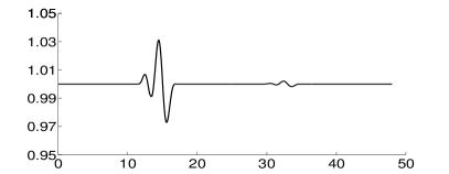
Figure 1. Burgers’ equation: Left boundary data for perturbed stationary shock.

The functional $J(u)$ is a weighted mean value in space and time of the solution,

$$J(u):=\int_{0}^{T}\int_{0.25}^{0.65}u(x,t)\exp\left(-\frac{1}{1-y(x)^{2}}\right)dxdt,$$

where $y(x):=(x-0.45)/0.2$. Note that the integration area completely covers the domain containing the shock.

4.2.1. Asymptotic decay rates

Since the adaptive strategy outlined in Section 4.1 above depends on assumptions on the assymptotic behavior of the error, we first try to estimate these decay rates. There is no analytical result which shows how the error terms $\bar{\eta}_{k}$ and $\bar{\eta}_{h}$ depend on $k$ and $h$. Therefore, we estimate this dependence numerically. We compute the perturbed shock described in Section 4.2 with a first order finite volume method with Engquist-Osher flux, which is equal to a DG(0,0) method. We compare the two approaches:

• refinement only time

• and refinement only space.

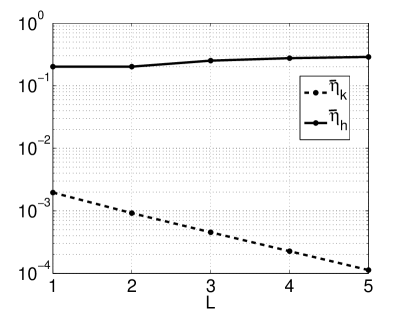
(a) uniform refinement in time

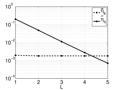
(b) uniform refinement in space

Figure 2. Error representation for Burgers equation, first order method, $\bar{\eta_{k}}$ and $\bar{\eta_{h}}$ versus level of refinement. (a) uniform refinement in time. (b) uniform refinement in space.

$L$	$dx$	$dt$	$\bar{\eta_{k}}$	$\bar{\eta_{h}}$	$\eta_{k}$	$\eta_{h}$	$J(u_{h})$	$\eta_{h}+\eta_{k}$	$\theta$
1	0.050000	0.038795	1.96e-03	2.02e-01	1.29e-04	2.00e-01	1.72e+00	2.01e-01	5.57e+00
2	0.025000	0.019398	9.81e-04	4.83e-02	1.83e-05	4.75e-02	1.74e+00	4.75e-02	5.49e+00
3	0.012500	0.009699	4.81e-04	1.21e-02	3.57e-06	1.17e-02	1.75e+00	1.17e-02	5.71e+00
4	0.062550	0.004849	2.37e-04	3.10e-03	1.30e-06	2.89e-03	1.75e+00	2.89e-03	7.06e+00

Table 1. Efficiency $\theta=\frac{\eta_{h}+\eta_{k}}{J(u)-J(u_{h})}$of the error representation

Each of the plots in Figure 2 show the error estimators $\bar{\eta}_{k}$ (error in time) and $\bar{\eta}_{h}$ (error in space). In the Figure 2(a) we refined only in time. Here the spatial error remains constant, while the time error still decreases with first order. The second Figure 2(b) shows the refinement only in space. The time error $\bar{\eta}_{k}$ is almost constant, while the spatial error is decreasing with second order.

Numerically the terms $\bar{\eta}_{t}$ and $\bar{\eta}_{h}$ behave as expected. They depend either on $k$ or on $h$, but never on both. The behaviour of $\eta_{h}$ and $\eta_{k}$ is very similar, and not displayed here.

Remark 5.

The numerically validated results can be used for adaptive grid refinement. The error estimator $\bar{\eta}_{h}$ can be used as an indicator for spatial adaption and the estimator $\bar{\eta}_{k}$ for time step control.

4.3. Computational results

Example 1: The first computation ($L=0$) is done on a grid with 20 spatial cells and a uniform CFL number of 0.8 using explicit timesteps. It needs $N=1238$ timesteps, reaching a total error of $\bar{\eta}=0.204$ and a relative error of $|\bar{\eta}/J(u_{h})|=11.9\%$, but a temporal error of $|\bar{\eta}_{k}/J(u_{h})|=0.13\%$. Our adaptive strategy now aims at a time step distribution on the next grid with tolerance $T\!ol_{k}(L+1)=\bar{\eta}_{k}(L)$. Based on the assumption that the time component of the error varies linearly with the time step (which is motivated by Fig. 2), the scheme chooses new timesteps on the next grid according to the equidistribution rule (34).

The second row of Table 2, for level $L=1$, gives also $N=1238$ time steps, now using adaptive implicit timesteps. Now the relative temporal error is $|\bar{\eta}_{k}/J(u_{h})|=0.073\%$, and it is dominated by the spatial error $|\bar{\eta}_{h}/J(u_{h})|=2.2\%$.

L	N	$\bar{\eta}_{k}/J(u_{h})$	$\bar{\eta}_{h}/J(u_{h})$	$\bar{\eta}/J(u_{h})$
0	1238	1.34e-03	1.17e-01	1.19e-01
1	1238	7.37e-04	2.20e-02	2.27e-02

Table 2. Example 1: Perturbed shock for Burgers’ equation. From left to right: level $L$, number of time steps $N$, time component of error estimator $\bar{\eta}_{k}/J(u_{h})$, spatial component of error estimator $\bar{\eta}_{h}/J(u_{h})$, total error estimator $\bar{\eta}/J(u_{h})$.

Important additional information can be gained by looking at the plots in Figure 3, showing the CFL distribution on each time interval $I_{n}$ and the normalized time components of the error estimator $\bar{\eta}_{k}^{n}$, both in logarithmic scale. The stationary and instationary regions are separated by the estimator. In particular, note that

• the time component of the error varies over more than 14 orders of magnitude.

• in the three stationary regions, $\bar{\eta}_{k}^{n}$ is very close to zero.

• the two instationary waves are distinguished very clearly. The second wave is about one order of magnitude smaller than the first wave. This corresponds closely to the different magnitudes of the inflow perturbations.

• furthermore, one can clearly identify an initial layer, where $\bar{\eta}_{k}^{n}=\mathcal{O}(1)$ at the inflow boundary $t=0$, and $\bar{\eta}_{k}^{n}$ decays exponentially for time $t>0$ until it reaches machine accuracy.

We advance to level $L=1$, Figures 3(c) and (d). We observe that

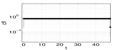
(a) $C\!F\!L(t_{n})$, L=0, uniform explicit timestep

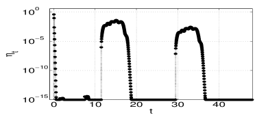
(b) $\bar{\eta}_{k}^{n}(t_{n})$, L=0, uniform explicit timestep

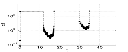
(c) $C\!F\!L(t_{n})$, L=1, adaptive implicit timestep

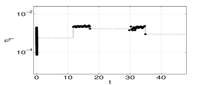
(d) $\bar{\eta}_{k}^{n}(t_{n})$, L=1, adaptive implicit timestep

Figure 3. Example 1: Perturbed shock for Burgers’ equation with equidistributed time error. Left column: CFL(t); right column: $\bar{\eta}_{k}^{n}(t_{n})$. Upper row: level $L=0$, fully explicit scheme, uniform timestep. Lower row: level $L=1$, fully implicit scheme, adaptive timestep. (from top to bottom).

• the error on level $L=1$ varies by less than 2 orders of magnitude, 12 orders of magnitude less than on level $L=0$. The magnitude of the maximal error has decreased by almost two orders of magnitude. Therefore the solution is much better resolved in the instationary regions, and the computational recources are clearly distributed more efficiently.

• in the initial layer, the CFL number starts with $\mathcal{O}(10^{-2})$. Then it grows at least exponentially until it reaches a maximal value of about 500. At the same time, the error $\bar{\eta}_{k}^{n}$ decays roughly by two orders of magnitude. Thus, these initial steps can be seen as a preprocessing of the initial data, to translate a prescribed steady shock on the pde level into a steady discrete shock layer. The initial layer is also clearly visible in the plot of the error distribution (and this will never disappear). Indeed, the initial data, a sharp jump from 1 to -1, are a steady shock only on the level of the exact solution. Numerically, the scheme has to converge towards a discrete shock layer, and this will always need a few time steps. In fact this is an instance of a scheme converging towards a numerical steady state solution, using adaptive time steps.

• in the stationary region between the initial layer and the first perturbation, the error is more than three orders of magnitudes smaller than in the following flow field. Observe that the whole stationary region is computed by a single time step. Thus the scheme is only held back from choosing a larger time step by the appearance of the instationary perturbation. If we had introduced this perturbation at a later time, the time step and thus the local CFL number would haves been correspondingly larger.

• The next region of stationary flow is again bridged by a single time step, and correspondingly the local error is somewhat below the equidistributed one.

• For the two perturbations, the normalized error is already close to being uniformly distributed.

• Using large timesteps does not mean that each timestep has higher computational costs. Since the adaptation chooses large timesteps, where the solution is(nearly) stationary, these timesteps have low computational costs.

We would also like to point out one drawback of the equidistribution strategy for the timestep. In the first (and larger) instationary wave, the proposed CFL number is often much smaller than unity, e.g. $\min\limits_{n}(C\!F\!L(t^{n}))=0.009$ in Figure 3. It is well-known that lowering the CFL number much below unity smears the solution. Therefore, while such small timesteps may improve the temporal accuracy somewhat, they will deteriorate the spatial accuracy considerably. Moreover, they increase the number of timesteps, and hence the computational cost. In the following example, we discuss a more efficient strategy.

Example 2: This example is a modification of the first example which used a fully implicit strategy for the timestep. Here we introduce a mixed implicit/explicit strategy. We still want the equidistribute the error, but we will give up this goal partially when the local $C\!F\!L$ number drops below a certain threshhold.

As discussed above, choosing timestep sizes with $C\!F\!L$ much less than unity seems to be inefficient both for explicit and for implicit schemes. For implicit methods, even timesteps with $C\!F\!L<5$ are not efficient, since we have to solve a nonlinear system of equations at each timestep. Thus, the new implicit/explicit strategy switches to the cheaper (and less dissipative) explicit method, if $C\!F\!L<5$, computing perhaps a few more timesteps if $0.8<C\!F\!L<5$, and saving timesteps if $C\!F\!L<0.8$. (Of course, we could choose other thresholds than $C\!F\!L=0.8$ and 5.)

As we can see in Table 3, the new strategy requires only 449 timesteps, instead of 1238 with the direct equidistribution in Example 1. Out of these, only 166 are implicit and hence expensive. This leads to considerable speed-up.

L	N(expl)	$\bar{\eta}_{k}/J(u_{h})$	$\bar{\eta}_{h}/J(u_{h})$	$\bar{\eta}/J(u_{h})$
1	449 (283)	8.50e-04	2.14e-02	2.23e-02

Table 3. Example 2: Same as Table 2, but CFL restriction from below (implicit/explicit strategy).

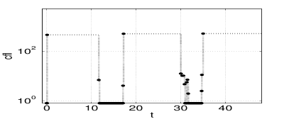
(a) $C\!F\!L(t_{n})$, L=1, adapt. impl./expl. timestep

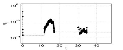
(b) Error $\bar{\eta}_{k}^{n}$, L =1, adapt. impl./expl. timestep

Figure 4. Example 2: Same as Figure 3 but adaptive implicit/explicit strategy (CFL restriction from below).

Example 3: Table 4 and Figure  5 show three extensions of Example 2. We used the same implicit/explicit strategy as in Example 2, but after the explicit reference computation on the coarse grid (L=0, error $\bar{\eta}_{k}^{ref}$), we proceed directly to a finer grid with 320 cells (L=4). We compare an explicit and two implicit/explicit computations on the fine grid.

The first row shows results of the fully explicit scheme with uniform refinement in time and space for L=4. As expected, the errors are about $2^{4}$ times smaller than those on the original coarse grid. Now suppose we wanted to reach comparable errors on level $L=4$ using adaptive timestepping. Then we should set the tolerance to be $\;T\!ol(4)=2^{-4}\bar{\eta}_{k}^{ref}\,$. The results of this computation are shown in the second row of Table 4. The three components of the error are comparable with those of the fully explicit computation, but the number of timesteps is only 3975 instead of 19200. Out of these 3975 steps, only 1235 are implicit.

Another strategy for equidistributing the error might be to fix any constant tolerance, for example $T\!ol(4)=\bar{\eta}_{k}^{ref}$ itself. The results of this computation are displayed in the last row of the table. The error in time is now a factor 5-8 higher than for the other two computations, while the spatial error is comparable. Remarkably, this computation needs only 1780 timesteps, and only 507 of these are implicit.

Both of these calculations show that considerable savings are possible with the implicit/explicit, time-adaptive strategy.

strategy	$T\!ol_{k}$	N(expl)	$\bar{\eta}_{k}/J(u_{h})$	$\bar{\eta}_{h}/J(u_{h})$	$\bar{\eta}/J(u_{h})$
fully expl.	–	19200 (19200)	7.11e-05	4.57e-04	5.28e-04
impl./expl.	$2^{-4}\bar{\eta}_{k}^{ref}$	13975 1(2740)	1.06e-04	3.71e-04	4.77e-04
impl./expl.	$\bar{\eta}_{k}^{ref}$	11780 1(1243)	5.46e-04	3.66e-04	9.12e-04

Table 4. Example 3: Same as Table 3, but on level L =4 and with different tolerances.

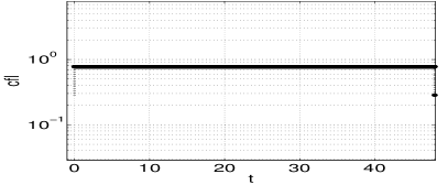
(a) $C\!F\!L(t_{n})$, uniform explicit

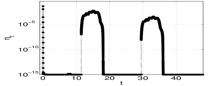
(b) $\bar{\eta}_{k}^{n}(t_{n})$, uniform explicit

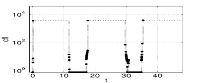
(c) $C\!F\!L(t_{n})$, adapt. impl./expl., $T\!ol_{k}=2^{-4}\bar{\eta}_{k}^{ref}$

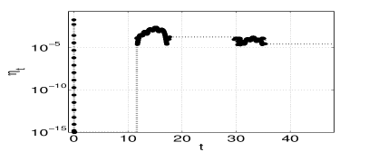
(d) $\bar{\eta}_{k}^{n}(t_{n})$, adapt. impl./expl., $T\!ol_{k}=2^{-4}\bar{\eta}_{k}^{ref}$

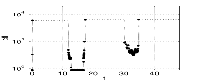
(e) $C\!F\!L(t_{n})$, adapt. impl./expl., $T\!ol_{k}=\bar{\eta}_{k}^{ref}$

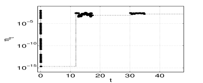
(f) $\bar{\eta}_{k}^{n}(t_{n})$, adapt. impl./expl., $T\!ol_{k}=\bar{\eta}_{k}^{ref}$

Figure 5. Example 3: Same as Figure 4 but on Level L =4 and with different tolerances.

5. Conclusions

In this paper, we combine space- and time-projections of Süli, Houston and Hartmann to split the classical adjoint based error representation formula for target functionals into space and time components. Based on a numerical study of these components we design an adaptive strategy which attempts to minimize the number of time steps by equidistributing the time components of the error. We apply the adaptive scheme to a weak perturbation of a stationary shock.

Already on a very coarse mesh of 20 points the error representation formula precisely gives the location and strength of the instationary perturbations. This can be translated into efficient timestep distributions, which respect a desired accuracy. We show that these timestep distributions can be applied successfully to much finer spatial grids.

We never compute implicit timesteps below CFL=5. Instead, when the error analysis suggests a timestep below CFL=5, we switch to an explicit scheme with CFL=0.8. This implicit/explicit strategy gives considerable savings.

For nonlinear perturbations of a stationary shock, we have demonstrated that our strategy does reach its goals: it separates initial layers, stationary regions and perturbations cleanly and chooses just the right timestep for each of them.

Besides building upon well-established adjoint techniques, we have also added a new ingredient which simplifies the computation of the dual problem. We show that it is sufficient to compute the spatial gradient of the dual solution, $w=\nabla\varphi$, instead of the dual solution $\varphi$ itself. This gradient satisfies a conservation law instead of a transport equation, and it can therefore be computed with the same algorithm as the forward problem, and in the same finite element space. For discontinuous transport coefficients, the new conservative algorithm for $w$ is more robust than our previous transport schemes for $\varphi$.

In ongoing work, we are adapting this strategy to aerodynamic problems. First test calculations show a promising speed-up.

Acknowledgement: The authors would like to thank Ralf Hartmann, Paul Houston, Mario Ohlberger and Endre Süli for stimulating discussions. The work of both authors was supported by DFG grant SFB 401 at RWTH Aachen. Part of the work was completed while the first author was in residence at the Center of Mathemtics for Applications (CMA) at Oslo University. Both authors would like to thank CMA its members for their generous hospitality.

References

- [1] T. Barth, H. Deconinck (ed.): Error Estimation and Adaptive Discretization Methods in Computational Fluid Dynamics, Vol. 25 in Lecture Notes in Computational Science and Engineering 25, Springer-Verlag, pp. 47–96, 2003.
- [2] T. Barth, M. Larson: A posteriori error estimates for higher order Godunov finite volume methods on unstructured meshes. In: R. Herbin, D. Kröner (ed.): Proceedings of “Finite volumes for complex applications III”. Porquerolles, June 24–28, 2002. Laboratoire d’Analyse, Topologie et Probabilités CNRS, Marseille, 2002.
- [3] F. Bramkamp, P. Lamby, S. Müller: An adaptive multiscale finite volume solver for unsteady and steady state flow computations. J. Comput. Phys. 197 (2004), 460–490
- [4] R. Courant, K.-O. Friedrichs, H. Lewy: Über die partiellen Differentialgleichungen der mathematischen Physik. Math. Ann. 100, pp. 32–74, 1928.
- [5] R. Becker, R. Rannacher: A feed-back approch to error control in finite element methods: basic analysis and examples. East-West J. Numer. Math 4, pp. 237–264, 1996.
- [6] R. Becker, R. Rannacher: An optimal control approach to error estimation and mesh adaptation in finite element methods. Acta Numerica 2000 (A. Iserles, ed.), pp. 1–102, Cambridge University Press, 2001.
- [7] B. Cockburn, S. Hou, C.-W. Shu: The Runge-Kutta local projection discontinuous Galerkin finite element method for conservation laws. IV. The multidimensional case. Math. Comp. 54, 545–581, 1990.
- [8] K. Eriksson, C. Johnson: Adaptive Finite Element Methods for Parabolic Problems I: A Linear Model Problem. SIAM J. Numer. Anal. 1991; 28: 43-77.
- [9] K. Eriksson, C. Johnson: Adaptive Finite Element Methods for Parabolic Problems II: Optimal Error Estimates in and . SIAM J. Numer. Anal. 1995; 32: 706-740.
- [10] K. Eriksson, C. Johnson: Adaptive Finite Element Methods for Parabolic Problems IV: Nonlinear Problems. SIAM J. Numer. Anal. 1995; 32: 1729-1749.
- [11] K. Eriksson, C. Johnson: Adaptive Finite Element Methods for Parabolic Problems V: Long-time integration. SIAM J. Numer. Anal. 1995; 32: 1750-1763.
- [12] K. Eriksson, C. Johnson, S. Larsson: Adaptive Finite Element Methods for Parabolic Problems VI: Analytic Semigroups. SIAM J. Numer. Anal. 1998; 35: 1315-1325.
- [13] R. Hartmann: A posteriori Fehlerschätzung und adaptive Schrittweiten- und Ortsgittersteuerung bei Galerkin-Verfahren für die Wärmeleitungsgleichung. Diplomarbeit, Institut für Angewandte Mathematik, Universität Heidelberg, 1998.
- [14] R. Hartmann, P. Houston: Adaptive Discontinuous Galerkin Finite Element Methods for Nonlinear Hyperbolic Conservation Laws. SIAM J. Sci. Comput. 24, pp. 979–1004, 2002.
- [15] R. Hartmann, P.Houston: Adaptive discontinuous Galerkin finite element methods for the compressible Euler equations. J. Comput. Phys. 183, 508–532, 2002.
- [16] J. Hoffman, C. Johnson: Adaptive finite element methods for incompressible fluid flow. In T. Barth, H. Deconinck (ed.), see [1], pp. 97–157, 2003.
- [17] D. Kröner, M. Ohlberger, A posteriori error estimates for upwind finite volume schemes for nonlinear conservation laws in multi dimensions. Math. Comp. 69 (2000), 25-39.
- [18] M. Ohlberger, A posteriori error estimate for finite volume approximations to singularly perturbed nonlinear convection-diffusion equations. Numer. Math. 87 (2001) 4, 737-761.
- [19] E. Süli: A posteriori error analysis and adaptivity for finite element approximations of hyperbolic problems. In: D. Kroener, M. Ohlberger and C. Rohde (Eds.) An Introduction to Recent Developments in Theory and Numerics for Conservation Laws. Lecture Notes in Computational Science and Engineering. Vol. 5, pp. 123–194, 1998,
- [20] E. Süli, P. Houston: Adaptive Finite Element Approximations of Hyperbolic Problems. In T. Barth, H. Deconinck (ed.), see [1], pp. 269–344, 2003.
- [21] E. Tadmor: Local error estimates for discontinuous solutions of nonlinear hyperbolic equations. SIAM J. Numer. Anal. 28, 891–906, 1991.