A method to retrieve optical and geometrical characteristics of three layer waveguides from m-lines measurements.

Abstract

We consider three layer optical waveguides and present a method to measure simultaneously the refractive index and the thickness of each layer with m-lines spectroscopy. We establish the three layer waveguide modal dispersion equations and describe a numerical method to solve these equations. The accuracy of the method is evaluated by numerical simulations with noisy data and experimentally demonstrated using a PZT thin film placed between two ZnO layers.

I Introduction

The considerable progress in thin film etching allows today the realization of almost any waveguide structure requiring submicron resolution. For example, the fabrication of single mode optical waveguides, couplers, interferometers or ring resonators is well controlled. Whatever their function, these structures are made of a superposition of several thin layers and they have to guide light. Therefore it is essential to accurately characterize the optical and geometrical properties of each layer of the stack. Several techniques exist to perform such a characterization in the case of a single layer film, such as those based on the measurements of the reflection and transmission coefficients of the sample Abelès (1963); Manifacier et al. (1976); Martínez-Antón (2000), the ellipsometry Azzam and Bashara (1977), and the m-lines spectroscopy Tien and Ulrich (1970); Ulrich (1970); Ulrich and Torge (1973). The case of multilayer waveguides has been much less investigated, although the assumption that a layer in a stack shows the same properties as it has when measured individually, can become wrong. The characterization of the whole structure then becomes necessary. Some work was done on the case of two layers Tien et al. (1973); Stutius and Streifer (1977); Hewak and Lit (1987); Matyás̆ et al. (1991); Aarnio et al. (1995); Kubica (2002) (sometimes denoted as a ”four layer film” since the stack is deposited on a substrate and the air is considered as a top layer), however, no literature is available for three layer structures. These structures are of special interest since they consist of the minimum number of layers required in order to obtain a single mode waveguide which is thick enough to enable efficient coupling of the light. In this paper we will focus on three layer waveguides and show how the refractive indices and thicknesses of the individual layers can be retrieved simultaneously from m-lines spectroscopy measurements.

In classical m-lines devices, the sample is pressed against a face of a prism. The prism and the film are mounted on a rotating stage in order to allow the variation of the light incidence angle. A thin air gap between the sample and the prism face is maintained whose thickness should be approximately the fourth of the light probe wavelength. The incoming light is refracted inside the prism and reaches the interface between the prism and the sample. Since the refractive index of the prism is higher than that of the sample, the light is totally reflected at this interface, for a given range of incidence angles, and then emerges from the prism to be detected. For some angles, called ”synchronous angles”, however, part of the light is coupled into the waveguide, hence substracted from the detected light. Therefore, a typical m-lines spectrum consists in several absorption-like peaks, centered around the synchronous angles. From the positions of the synchronous angles, it is possible to deduce the propagation constants of the guided modes of the sample under test and derive the optical and geometrical properties of the structure (refractive index and thickness) by solving the modal dispersion equations.

The first part of this paper is devoted to the determination of the explicit form of modal dispersion equations of the three layer waveguide. We will then describe the numerical method used in order to solve these equations and present numerical tests that prove its accuracy. The validity of the method will be finally demonstrated experimentally by the analysis of m-lines spectra produced by three layer ZnO/PZT/ZnO waveguides.

II Three layer dispersion equations

The studied structure is a stack of five transparent homogeneous layers shown on Fig. 1.

Figure 1: Three layer waveguide.

The substrate (layer #0) and the superstrate (layer #5) are considered as semi-infinite since their thicknesses are several orders of magnitude greater than those of layers $1$, $2$ and $3$. The light is confined only in these three central layers and presents an evanescent decay in the substrate and the superstrate. We call this structure a ”three layer waveguide”, whereas in the nomenclature of other authors Hewak and Lit (1987) it would be called a ”5 layer waveguide”. The central layer (layer #2) is the core of the structure and the layers #1 and #3 are the claddings (true waveguide Zhang et al. (2002)). As a consequence, we assume for the refractive indices of the different layers that:

$$n_{2}>n_{1},n_{3}>n_{0},n_{4}$$ (1)

In the following, we will restrict ourselves to the case of TE modes, the extension to the case of TM modes is straightforward. The only component of the electrical field of the TE modes is along the (Oy) axis, so the electric field in the layer j can be written as: $E_{yj}(x,z)=A_{j}\exp[i(\gamma_{j}x+\beta_{m}z)]+B_{j}\exp[i(-\gamma_{j}x+\beta_{m}z)]$ and the tangential component of the magnetic field is $H_{zj}(x,z)=i(\omega\mu_{0})^{-1}\partial E_{yj}/\partial x$. In these expressions, $\omega$ is the angular frequency and $\beta_{m}$ is the propagation constant of the $m^{\rm th}$ guided mode. It is usually written as $\beta_{m}=kN_{m}$, where $k$ is the wavevector modulus in vacuum and $N_{m}$ the effective index of the m^th mode. Using the condensed notation $a_{j}=k\ |n_{j}^{2}-N^{2}|^{1/2}$, the x component of the wavevector, $\gamma_{j}$, which gives the nature of the wave in the layer $j$, becomes $\gamma_{j}=(\omega\mu_{0})^{-1}a_{j}$ for a travelling wave and $\gamma_{j}=i(\omega\mu_{0})^{-1}a_{j}$ for an evanescent wave. A transfer matrix $M_{j}$, which binds the electromagnetic fields at the backplane of the layer to the fields at its frontplane, can be associated to each layer Chilwell and Hodgkinson (1984):

$$M_{j}=\left(\begin{array}[]{cc}\cos(\omega\mu_{0}\gamma_{j}d_{j})&\displaystyle\frac{i}{\gamma_{j}}\sin(\omega\mu_{0}\gamma_{j}d_{j})\\ i\ \gamma_{j}\sin(\omega\mu_{0}\gamma_{j}d_{j})&\cos(\omega\mu_{0}\gamma_{j}d_{j})\\ \end{array}\right)$$ (2)

The boundary conditions imply that the tangential components of the magnetic and electrical fields must be continuous at the interface of the layers. These conditions together with the condition for obtaining guiding lead to:

$$\left(\begin{array}[]{c}1\\ -\gamma_{4}\end{array}\right)E_{4y}=M_{3}M_{2}M_{1}\left(\begin{array}[]{c}1\\ \gamma_{0}\end{array}\right)E_{0y}=M\left(\begin{array}[]{c}1\\ \gamma_{0}\end{array}\right)E_{0y}$$ (3)

which has solutions only for:

$$\gamma_{4}m_{11}+\gamma_{4}\gamma_{0}m_{12}+m_{21}+\gamma_{0}m_{22}=0$$ (4)

where $m_{ij}$ are the components of the matrix $M$. With the definition (2) of the transfert matrix, this equation can be written as Schneider (2006):

$$\begin{array}[]{ll}{a_{2}}\,{d_{2}}&+\;{\rm arctan}\left[\!{\displaystyle\frac{i\gamma_{0}\,\gamma_{1}+\gamma_{1}^{2}\,{\tan}({\omega\mu_{0}\gamma_{1}}\,{d_{1}})}{\gamma_{1}\,\gamma_{2}-i{\displaystyle\gamma_{0}\,\gamma_{2}\,\tan({\omega\mu_{0}\gamma_{1}}\,{d_{1}})}}}\!\right]\\[22.76219pt] &+\;{\rm arctan}\left[\!\displaystyle\frac{i\gamma_{3}\,\gamma_{4}+\gamma_{3}^{2}\,\tan({\omega\mu_{0}\gamma_{3}}\,{d_{3}})}{\gamma_{2}\,\gamma_{3}-i\gamma_{2}\,\gamma_{4}\,\tan(\omega\mu_{0}{\gamma_{3}}\,{d_{3}})}\!\right]-\;m\,\pi=0\end{array}$$ (5)

which is the general modal dispersion equation for the true three layer waveguides.

As stated above, the $\gamma_{j}$ terms are either real or imaginary depending on the nature of the waves in the $j^{\rm th}$ layer. As a consequence, an analysis in the complex plane is required in order to solve directly the equation 5. It is better to take advantage of physical arguments to split the problem in several simpler ones. Under the condition of Eq. 1, three kinds of guided waves can exist:

• The lowest order modes can only propagate in the layer #2. Then $\gamma_{2}$ only is real and Eq. 5 becomes:

  $$\begin{array}[]{l}{a_{2}}\,{d_{2}}-\;\mathrm{arctan}\left[\!{\displaystyle\frac{a_{0}\,a_{1}+a_{1}^{2}\,\mathrm{tanh}({a_{1}}\,{d_{1}})}{a_{1}\,a_{2}+{\displaystyle a_{0}\,a_{2}\,\mathrm{tanh}({a_{1}}\,{d_{1}})}}}\!\right]\\[11.38109pt] \quad-\;\mathrm{arctan}\left[\!\displaystyle\frac{a_{3}\,a_{4}+a_{3}^{2}\,\mathrm{tanh}({a_{3}}\,{d_{3}})}{a_{2}\,a_{3}+a_{2}\,a_{4}\,\mathrm{tanh}({a_{3}}\,{d_{3}})}\!\right]-\;m\,\pi=0\end{array}$$ (6)

• As the order of the mode increases, the wavevector approaches the normal of the interfaces. For a given mode $m_{2}$, the incidence angle on the interface between the central layer and one cladding layer becomes smaller than the limit angle for total internal reflection and the light propagates inside these two layers. If $n_{3}>n_{1}$ then the light is guided in the layers #2 and #3 and Eq. 5 becomes:

  $$\begin{array}[]{l}{a_{2}}\,{d_{2}}-\;\mathrm{arctan}\left[\!\displaystyle\frac{a_{0}\,a_{1}+a_{1}^{2}\,\mathrm{tanh}({a_{1}}\,{d_{1}})}{a_{1}\,a_{2}+a_{0}\,a_{2}\,\mathrm{tanh}({a_{1}}\,{d_{1}})}\!\right]\\[11.38109pt] \quad-\;\mathrm{arctan}\left[\displaystyle\!\frac{\displaystyle a_{3}\,a_{4}-a_{3}^{2}\,\mathrm{tan}({a_{3}}\,{d_{3}})}{\displaystyle a_{2}\,a_{3}+a_{2}\,a_{4}\,\mathrm{tan}({a_{3}}\,{d_{3}})}\!\right]-\;m\,\pi=0\end{array}$$ (7)

  Otherwise, the light propagates in the layers #1 and #2. The corresponding modal dispersion equation is obtained by interverting the functions $\tan$ and $\tanh$ in Eq. 7.

• Finally, highest order modes can propagate in the three layers. The dispersion equation for these modes is:

  $$\begin{array}[]{l}{a_{2}}\,{d_{2}}-\;\mathrm{arctan}\left[\!\displaystyle\frac{a_{0}\,a_{1}-a_{1}^{2}\,\mathrm{tan}({a_{1}}\,{d_{1}})}{a_{1}\,a_{2}+a_{0}\,a_{2}\,\mathrm{tan}({a_{1}}\,{d_{1}})}\!\right]\\[11.38109pt] \quad-\;\mathrm{arctan}\left[\displaystyle\!\frac{\displaystyle a_{3}\,a_{4}-a_{3}^{2}\,\mathrm{tan}({a_{3}}\,{d_{3}})}{\displaystyle a_{2}\,a_{3}+a_{2}\,a_{4}\,\mathrm{tan}({a_{3}}\,{d_{3}})}\!\right]-\;m\,\pi=0\end{array}$$ (8)

III Data analysis : algorithm and numerical tests

At a first glance, the problem contains 6 unknown parameters which are the refractive indices and thicknesses of the layers #1, 2 and 3.

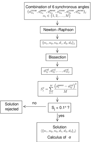
Figure 2: Algorithm of the resolution of the system of 6 equations in 6 unknowns and $M$ measured modes.

However, depending on the guiding regime, one has to associate correctly the dispersion equation to each measured synchronous angle. Consequently, further parameters have to be determined:

• $m_{1}$, the order of the first measured mode. It is often equal to 0, but the lower order modes are sometimes difficult to excite, and hence may be not visible in the m-lines spectrum. There is no evidence on the value of $m_{1}$ in practice.

• $m_{2}$, the order of the first mode guided by two layers. Numerical simulations with noisy data showed that $m_{2}$ is the value of $m$ such that $|N_{m}-N_{m-1}|>|N_{m+1}-N_{m}|$. This criterion results in a correct value of $m_{2}$ or with a mismatch of +1 Schneider et al. (2007). In the following we will call $m_{2}^{\rm th}$ the value given by this criterion.

• $m_{3}$, the order of the first mode guided by three layers.

• Finally, the modal dispersion equation in the case of two guiding layers is not the same according to whether $n_{1}$ is smaller or greater than $n_{3}$. Hence it is also necessary to make an initial hypothesis on the relative values of $n_{1}$ and $n_{3}$ and to verify this assumption during the resolution.

The analysis of a m-lines spectrum thus requires a somewhat complicated algorithm. For clarity reasons, we splitted the presentation of this algorithm into two parts (Fig. 2 and 3).

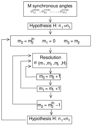
Figure 3: Algorithm of the m-lines spectra analysis.

Figure 4: Distribution of errors on the parameter $n_{2}$.

The details of the ”resolution” box of the full algorithm (shown on Fig. 3) are presented in Fig. 2, aiming to solve a system of 6 equations in 6 unknowns for $m_{1}$, $m_{2}$, $m_{3}$ given and for an assumption on the relative values of $n_{1}$ and $n_{3}$. Obviously, this problem can be solved only if the m-lines spectrum contains more than 6 modes. Let us call $M$ the number of measured synchronous angles. There is $C_{6}^{M}$ combinations of 6 modes. For a given combination $j$, we firstly use a Newton-Raphson method to get a solution $\{n_{1},n_{2},n_{3},d_{1},d_{2},d_{3}\}_{j}$. Then, we start from this solution and use a bissection algorithm to calculate the set of $M$ corresponding synchronous angles : $\{\phi_{ij}^{\rm cal}\}$, $i\in\{1,2,\dots,M\}$. The validity of the solution is evaluated by the standard deviation of the differences between the values of the calculated synchronous angles and the measured ones:

$$S_{j}^{2}=\sum_{i=1}^{M}\displaystyle\frac{\left(\phi_{i}^{\rm meas}-\phi_{ij}^{\rm cal}\right)^{2}}{M}$$ (9)

If $S_{j}$ is smaller than $0.1^{\circ}$ (upper limit of experimental uncertainty), the solution is considered as correct. This procedure is used for the $C_{6}^{M}$ combinations but it does not find roots in all cases. Let us call $\Gamma$ the number of combinations for which the procedure succeeds. The solution we finally retain is the mean value of these $\Gamma$ solutions and we associate a fitness $\sigma$ to this solution defined by:

$$\sigma^{2}=\sum_{j=1}^{\Gamma}\frac{S_{j}^{2}}{\Gamma^{2}}$$ (10)

$\Gamma^{2}$ was used rather than $\Gamma$, in order to give more weight to the configurations which lead to a high number of acceptable solutions.

The parameters $m_{1}$, $m_{2}$, and $m_{3}$ are obtained with an iterative procedure schematized on Fig. 3. We start with the $M$ measured synchronous angles and under the hypothesis $H:n_{1}>n_{3}$. The value of $m_{2}$ is set to $m_{2}^{\rm th}$, $m_{1}$ to 0 and $m_{3}$ to $m_{2}$ and the procedure of resolution described above is used in order to get a solution and its associated fitness $\sigma_{H,m_{1},m_{2},m_{3}}$. This procedure is repeated with firstly an incrementation of $m_{3}$ from $m_{2}$ to $M$, secondly an incrementation of $m_{1}$ from 0 to 5 (which in general is sufficient) and thirdly by setting $m_{2}$ to $m_{2}^{\rm th}-1$. For the case where no solution was obtained at the end of these iterations, the whole procedure is repeated with the opposite hypothesis ($n_{1}<n_{3}$). The refractive indices and thicknesses finally selected are those which are associated to the lowest value of $\sigma$ thus defining the values $m_{1}$, $m_{2}$, $m_{3}$ and $H$.

The validity of the method was verified by numerical simulations. Starting from a theoretical waveguide defined by the parameters $\{n_{1}^{\rm th},n_{2}^{\rm th},n_{3}^{\rm th},d_{1}^{\rm th},d_{2}^{\rm th},d_{3}^{\rm th}\}$, we calculated the corresponding set of synchronous angles $\{\phi_{i}^{\rm th}\},\ 0\leq i\leq 8$. In order to test the sensitivity to the noise, this set was used for building one hundred sets of noisy data $\{\phi_{i}^{\rm noisy}\}$ by adding to each theoretical synchronous angle, $\phi_{i}^{\rm th}$, a random value, $\varepsilon_{i}$, standing in the interval $[-\delta\phi,\delta\phi]$ with a uniform probability density. The values of $\delta\phi$ used in the simulations were chosen in order to correspond to the experimentally observed noise.

The hundred noisy data sets were analysed, giving rise to a number $\Lambda$ of sets of solutions $\{n_{1}^{\rm sol},n_{2}^{\rm sol},n_{3}^{\rm sol},d_{1}^{\rm sol},d_{2}^{\rm sol},d_{3}^{\rm sol}\}$. $\Lambda$ depends on the magnitude of the noise, it is very close to 100 for $\delta\phi=0.01^{\circ}$ and about 80 for $\delta\phi=0.1^{\circ}$. Each value $p^{\rm sol}_{j,\ 1\leq j\leq\Lambda}$ of the parameter $p$ ($p=n_{1},n_{2},n_{3},d_{1},d_{2}$ or $d_{3}$) differed from the theoretical value $p_{j}^{\rm th}$. The distribution of errors $\delta p_{j}=p_{j}^{\rm sol}-p_{j}^{\rm th}$ followed a normal law for all parameters $p$ and all noises Schneider (2006), as showed on Fig. 4 for the example of $n_{2}$. Finally, we defined the uncertainty $\Delta p$ on the parameter $p$ as three times the standard deviation of the distribution, in order to be in the confidence interval of 99%: $\Delta p=3\left[\sum_{j=1}^{\Lambda}\Lambda^{-1}(\delta p_{j}-\langle\delta p\rangle)^{2}\right]^{1/2}$.

A total of eight thousands waveguides were simulated, whose characteristics are summarized in Tab. 1. The thickness of the upper layer, $d_{3}$, was constant and smaller than the penetration depth of the light, in order to make possible the evanescent coupling between the prism and the central layer.

Table 1: Range of parameters explored with the statistical study.

	Start	End	Step
$n_{1}$, $n_{3}$	1.6	$n_{2}$-0.1	0.1
$n_{2}$	1.7	2.4	0.1
$d_{1}$, $d_{2}$	1.0 $\mu$m	2.0 $\mu$m	0.1 $\mu$m
$d_{3}$	100 $nm$

In order to get global estimators, we studied the distribution of uncertainties $\Delta p$ of each parameter for $p$ for all the simulated guides and for each noise. It was always possible to fit the distribution with a log-normal law (see Fig. 5):

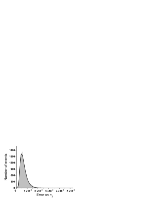
Figure 5: Distribution of the uncertainties $\Delta n_{2}$ over all the simulated guides, fitted by a lognormal law.

Figure 6: Evolution of the error on the refractive indices as a function of the noise on the synchronous angles.

$$f(\Delta p)=\frac{1}{w\Delta p\sqrt{2\pi}}\ {\rm e}^{\displaystyle-\frac{(\ln\Delta p-\mu)^{2}}{2w^{2}}}$$ (11)

where $w$ and $\mu$ are the free parameters of the model. Hence, the mean error was $\langle\Delta p\rangle=\exp\left(\mu+w^{2}/2\right)$ and the standard deviation of the distribution was: $\sigma_{\Delta p}^{2}=\left(\exp({w^{2}})-1\right)\exp(2\mu+w^{2})$. It followed that 85% of the errors were in the range $\langle\Delta p\rangle\pm\sigma_{\Delta p}$. We then used $\langle\Delta p\rangle$ as an estimate of the error on the parameter p with an uncertainty $\sigma_{\Delta p}$.

The results of the simulations are summarized on the graphics of Fig. 6 and Fig. 7. For the central layer, the error on the refractive index is lower than $1\times 10^{-3}$ and the error on the thickness remains lower than ten nanometers for a noise on the synchronous angles below 0.1^∘. For the other layers the errors on the refractive indices remain acceptable. They are smaller than $1\times 10^{-3}$ for the layer #1 and of the order of $1\times 10^{-2}$ for the upper layer. Nethertheless, the errors on the thicknesses can reach large values, especially for $d_{3}$. However, it should be emphasized that the number of synchronous angles used for the statistical study was limited to 9 in order to limit the computation time. A closer inspection of the guides leading to unaccurate results showed that the accuracy can be considerably enhanced when increasing the number of modes taken into account. As an example, Fig 8 and Fig 9 show the evolution of the errors on the different parameters as a function of the number of modes for a noise of 0.01^∘ and a guide defined by $n_{1}=1.9$, $n_{2}=2.3$, $n_{3}=2.2$, $d_{1}=1.1\ \mu$m, $d_{2}=1.9\ \mu$m, and $d_{3}=100$ nm.

Figure 7: Evolution of the error on the thicknesses as a function of the noise on the synchronous angles.

The errors on $d_{1}$ and $n_{1}$ can be reduced by two orders of magnitude while the error on $d_{3}$ and $n_{3}$ is divided by 2 when the number of modes used in the calculation is increased from 9 to 15.

This means that one should always use the maximum number of modes in order to reach the best accuracy. However, the computation time also increases.

Figure 8: Evolution of the error on the refractive indices as a function of the number of synchronous angles used in the resolution.

IV Experimental results

In order to experimentally validate the method, several multilayer structures were elaborated. They were deposited on glass substrates and were composed of lead zirconate titanate (PZT) for the core layer and Al doped zinc oxide (ZnO) for the claddings. A SEM picture of one of these samples is shown on Fig. 10.

The zinc oxide layers were grown by RF magnetron sputtering at room temperature from a 3” in diameter ZnO/Al₂O₃ (98/2 wt.%) ceramic target. Prior to the deposition, a pressure lower than $5\times 10^{-7}$ mbar was reached and pure argon was used as a sputter gas at a partial pressure of $2\times 10^{-3}$ mbar during the deposition process. An on-axis growth rate of approximately 100 nm/min was achieved at a RF power of 200 W at a target-substrate distance of 7.5 cm. The films were annealed at 650^∘C during 3 min and cooled down to room temperature during 3 hours. Four substrates were placed side by side under the ZnO target, resulting in a non homogeneous thickness of the films.

Figure 9: Evolution of the error on the thicknesses as a function of the number of synchronous angles used in the resolution.

In the following we will call ”$A_{\ell}$” and ”$A_{r}$” the samples directly on the left and on the right side of the center of deposition, ”$B_{\ell}$” the sample on the left of $A_{\ell}$ and ”$B_{r}$” the sample on the right of $A_{r}$. For symmetry reasons, we expect ZnO layers $A_{\ell}$ and $A_{r}$ as well as $B_{\ell}$ and $B_{r}$, to be identical.

Figure 10: SEM photograph of a three layer waveguide.

The PZT 36/64 layers were elaborated by Chemical Solution Deposition technique Cardin et al. (2005). A modified Sol-gel process was used for the elaboration of the PZT precursor solution, which consisted of lead acetate dissolved in acetic acid, zirconium and titanium n-propoxide; ethylene glycol was added in order to prevent from crack formation during the annealing process. The final solution was spin-coated on the ZnO layer at 1000 rpm and a Rapid Thermal Annealing procedure at 650^∘C resulted in the formation of a polycrystalline perovskite without remaining pyrochlore phases. A layer of PZT was spin-coated individually on samples $A_{\ell}$, $A_{r}$, $B_{\ell}$ and $B_{r}$. After cristallisation, we expect a repeatability of $8\times 10^{-3}$ on the refractive index and of 20 nm on the thickness Cardin et al. (2005).

The upper ZnO cladding layer was only deposited on samples $A_{r}$ and $B_{r}$ with a thickness smaller than the penetration depth of the light. These two samples were not characterized, neither with m-lines nor with other technique, until the third layer was deposited, in order to avoid pollution or any other deterioration of the structure. The two layers waveguides $A_{\ell}$ and $B_{\ell}$ were used as control samples.

Another three layer sample, called ”C” in the following, was elaborated in the same way as the samples $A$ and $B$, but it was characterized by m-lines after each deposition step.

We first consider the samples $A$ and $B$. An example of m-lines spectrum, obtained with sample $B_{r}$, is shown on Fig. 11. The transition from the single guiding layer to the two guiding layer regime appears clearly in the spectrum. Indeed, the broad peaks correspond to the waves guided in the PZT layer only, while the narrow peaks are associated to the waves also guided in the ZnO. This broadening is not a peculiarity of the three layer structure, it can be also observed for PZT single layers and may be due to light diffusion resulting in a loss along the direction of propagation Zhang et al. (2002).

Figure 11: m-lines spectrum obtained with sample $B_{r}$ measured at 29 $mm$ from the center of deposition.

The transition from the two guiding layer regime to the three guiding layer regime can not be infered from the spectrum and has to be determined by numerical computation.

Figure 12: Evolution of the thicknesses of the different layers of the three layer samples $A_{r}$, $B_{r}$ ($d_{1}:\square$, $d_{2}:$ $\circ$, $d_{3}:\triangle$ ) and the two layer samples $A_{\ell}$, $B_{\ell}$ ($d_{1}:\blacksquare$, $d_{2}:$ $\bullet$).

The spectrum of Fig. 11 was analyzed with the numerical method described in section 2, resulting in the following characteristics:

• layer #1 : $n_{1}=1.9701\pm 6\times 10^{-4}$, $d_{1}=1.588\pm 3\times 10^{-3}\mu m$

• layer #2 : $n_{2}=22702\pm 6\times 10^{-4}$, $d_{2}=0.894\pm 6\times 10^{-3}\mu m$

• layer #3 : $n_{3}=2.037\pm 9\times 10^{-3}$, $d_{3}=0.122\pm 3\times 10^{-3}\mu m$

Due to the complexity of the system to solve, the uncertainties were estimated with Monte Carlo simulations, in a similar way to what is described in section 3. Starting from the solution $\{n_{1},n_{2},n_{3},d_{1},d_{2},d_{3}\}$, we calculated the associated synchronous angles $\{\phi_{i}\}$ and built one hundred sets of noisy angles by adding a random value in the range of the experimental uncertainties. We then computed the solutions corresponding to the differents noisy sets and considered their distributions. The uncertainty on each parameter is defined as three times the standard deviation of the distribution of the values of this parameter.

We performed m-lines measurements every 4 mm from the center of the ZnO deposition. Fig. 12 and Fig. 13 show respectively the evolution of the thickness and the refractive indices of the different layers of the samples $A$ and $B$. If we except the point located at 41 mm from the deposition center, where few modes were available due to the low thickness of the lower ZnO layer, the error bars do not clearly appear since the uncertainties are small. They are of the order of $5\times 10^{-4}$ for $n_{1}$ and $n_{2}$, and $1\times 10^{-2}$ for $n_{3}$.

Figure 13: Evolution of the refractive indices of the different layers of the three layer samples $A_{r}$, $B_{r}$ ($n_{1}:\square$, $n_{2}:$ $\circ$, $n_{3}:\triangle$ ) and the two layer samples $A_{\ell}$, $B_{\ell}$ ($n_{1}:\blacksquare$, $n_{2}:$ $\bullet$ ).

The uncertainties on the thicknesses are of the order of 10 nm, which corresponds to a relative accuracy of 0.5% for $d_{1}$ and $d_{2}$, and 10% for $d_{3}$. As expected, the thickness of the lower ZnO layers decreases with the distance from the ZnO deposition center (Fig. 12). The thickness of the PZT films is rather constant except at the border of the samples where a slight increase can be observed which is typical for the spin-coating process.

The refractive index of the PZT layer varies from 2.2227$\pm 5\times 10^{-4}$ to 2.3610$\pm 5\times 10^{-4}$. It is slightly higher than the refractive index of the PZT deposited on glass under the same conditions Cardin et al. (2005). This may be due to a structural change of the PZT thin film induced by the ZnO buffer layer which acts as a diffusion barrier thus hindering diffusion of the lead from the PZT into the glass substrate. The index of the ZnO lower layer is rather constant, it oscillates between 1.9667$\pm 6\times 10^{-4}$ and 1.991$\pm 5\times 10^{-3}$. On the contrary, the index of the upper ZnO layer exhibits strong variations from 2.015$\pm 8\times 10^{-3}$ to 2.123$\pm 8\times 10^{-3}$. This may be explained by the existence of two different cristalline structures arising when the thicknesses of the ZnO film is below 500 nm Lin and Huang (2004).

The differences between the thicknesses and refractive indices obtained for the three layer waveguides ($A_{r}$, $B_{r}$) and the two layer waveguides ($A_{\ell}$, $B_{\ell}$) essentially stay in the range of the repeatability of the elaboration procedure and the measurement techniques. So the method of analysis of three layer guides m-lines spectra gives results in accordance to those obtained with two layer guides. This is confirmed by the measurements realized from sample $C$, where the refractive index and the thickness of the layers where measured before and after deposition of the upper cladding layer. The results are summarized in Tab. 2 showing that the differences between the values obtained before and after the third deposition remain always smaller than the uncertainty and the repeatability of the elaboration procedure and the measurement techniques. This good agreement proves the validity of our method.

Table 2: Comparison of the measured characteristics of a waveguide (sample $C$), before and after the deposition of the upper cladding layer.

	$n_{1}$	$d_{1}$ ($\mu m$)	$n_{2}$	$d_{2}$ ($\mu m$)	$n_{3}$	$d_{3}$ ($\mu m$)
Two layers	1.978	1.11	2.360	1.02
Three layers	1.979	1.09	2.368	0.96	1.987	0.13

V Conclusion

In this paper, the general modal dispersion equation for a three layer planar waveguide is shown, from which the modal dispersion equations that hold for different guiding regimes are derived. A method to solve these equations is proposed, where the input data are the synchronous angles measured by m-lines spectroscopy. Monte Carlo simulations show that the values of the refractives indices and the thicknesses of the central layer given by this method are as accurate as those obtained for a single layer. The accuracy is not so good for the upper layer, however, the error remains smaller than 2.10^-2 for the index and below 30 nm for the thickness when the uncertainty on the measured angles remains smaller than 0.1^∘. The method was applied to the characterization of real three layer planar waveguide structures made of one PZT layer embedded between two ZnO cladding layers deposited on glass substrate. The agreement between the results obtained with three layer structures and those obtained with two layer structures ensures the validity of our method. Moreover, the three layer analysis revealed changes in material properties, such as increasing of the refractive index of PZT deposited on ZnO in comparison to deposition on glass and increasing of the refractive index of ZnO deposited on PZT in comparison to deposition on glass.

The proposed method allows to simultaneously characterize the optical and geometrical properties of each layer of three layer waveguides. Consequently, it is a very interesting instrument in order to verify whether the three layer structures are matching the parameters defined during the design process of waveguide.

References

- Abelès (1963) F. Abelès, Progress in Optics, vol. 2 (E. Wolf (North Holland), 1963).
- Manifacier et al. (1976) J. C. Manifacier, J. Gasiot, and J. P. Fillard, Journal of Physics E: Scientific Instruments 9, 1002 (1976).
- Martínez-Antón (2000) J. C. Martínez-Antón, Applied Optics 39, 4557 (2000).
- Azzam and Bashara (1977) R. Azzam and N. Bashara, Ellipsometry and Polarized Light (North Holland Publishing Company, 1977).
- Tien and Ulrich (1970) P. K. Tien and R. Ulrich, Journal of the Optical Society of America 60, 1325 (1970).
- Ulrich (1970) R. Ulrich, Journal of Optical Society of America 60, 1337 (1970).
- Ulrich and Torge (1973) R. Ulrich and R. Torge, Applied Optics 12, 2901 (1973).
- Tien et al. (1973) P. Tien, R. Martin, and G. Smolinsky, Applied Optics 12, 1909 (1973).
- Stutius and Streifer (1977) W. Stutius and W. Streifer, Applied Optics 16, 3218 (1977).
- Hewak and Lit (1987) D. W. Hewak and J. W. Y. Lit, Applied Optics 26, 833 (1987).
- Matyás̆ et al. (1991) M. Matyás̆, J. Bok, and T. Sikora, Physica Status Solidi (a) 126, 533 (1991).
- Aarnio et al. (1995) J. Aarnio, P. Kersten, and J. Lauckner, IEE Proc. Optoelectron. 142, 241 (1995).
- Kubica (2002) J. Kubica, Journal of Lightwave Technology 20, 114 (2002).
- Zhang et al. (2002) X.-J. Zhang, X.-Z. Fan, J. Liao, H.-T. Wang, N. B. Ming, L. Qiu, and Y.-Q. Shen, Journal of Applied Physics 92, 5647 (2002).
- Chilwell and Hodgkinson (1984) J. Chilwell and I. Hodgkinson, Journal of the Optical Society of America A 1, 742 (1984).
- Schneider (2006) T. Schneider, Ph.D. thesis, Université de Nantes (2006).
- Schneider et al. (2007) T. Schneider, D. Leduc, J. Cardin, C. Lupi, N. Barreau, and H. Gundel, Optical Materials 29, 1871 (2007).
- Cardin et al. (2005) J. Cardin, D. Leduc, T. Schneider, C. Lupi, D. Averty, and H. Gundel, Journal of the European Ceramic Society 25, 2913 (2005).
- Lin and Huang (2004) S. Lin and J. Huang, Surface & Coatings Technology 185 (2004).