A Blob Method for the Aggregation Equation

Abstract.

Motivated by classical vortex blob methods for the Euler equations, we develop a numerical blob method for the aggregation equation. This provides a counterpoint to existing literature on particle methods. By regularizing the velocity field with a mollifier or “blob function”, the blob method has a faster rate of convergence and allows a wider range of admissible kernels. In fact, we prove arbitrarily high polynomial rates of convergence to classical solutions, depending on the choice of mollifier. The blob method conserves mass and the corresponding particle system is both energy decreasing for a regularized free energy functional and preserves the Wasserstein gradient flow structure. We consider numerical examples that validate our predicted rate of convergence and illustrate qualitative properties of the method.

1. Introduction

The aggregation equation describes the evolution of a nonnegative density $\rho$ according a velocity field which is obtained by convolving the density with the gradient of a kernel $K:{\mathord{\mathbb{R}}^{d}}\to{\mathord{\mathbb{R}}}$,

(1.1) $$\begin{cases}\rho_{t}+\nabla\cdot(\vec{v}\rho)=0\ ,\quad\quad\quad\quad\vec{v}=-\nabla K*\rho\ ,\\ \rho(x,0)=\rho_{0}(x)\ .\end{cases}$$

The dynamics governed by this equation arise in a range of problems, including biological swarming [55, 54, 65, 66], robotic swarming [58, 26], molecular self-assembly [29, 67, 61], and the evolution of vortex densities in superconductors [2, 68, 49, 30, 53, 59]. For swarming and molecular self-assembly, common choices of kernel include the repulsive-attractive Morse potential and power law potential,

(1.2) $$K(x)=C_{r}e^{-|x|/l_{r}}-C_{a}c^{-|x|/l_{a}}\ ,\quad K(x)=|x|^{a}/a-|x|^{b}/b\ ,\quad a>b\ .$$

To model the evolution of vortex densities in superconductors, $K$ is chosen to be the two dimensional Newtonian potential,

(1.3) $$K(x)=\frac{1}{2\pi}\log|x|\ .$$

In addition to utility in a range of applications, the aggregation equation possesses several features of current mathematical interest. It is non-local—the motion of the density at any point depends on the value of the density at every point—and when $K$ is symmetric it is formally a gradient flow in the Wasserstein metric. When $K$ has low regularity at the origin, solutions may blow up in finite time or form rich patterns as they approach a steady state. In recent years, there has been substantial interest in these structures from both analytic and numerical perspectives [5, 4, 14, 6, 13, 12, 10, 11, 21, 23, 28, 34, 33, 36, 35, 44, 45, 48, 59, 60, 64, 65, 43]. For example, Kolokolnikov, Sun, Uminsky, and Bertozzi studied steady states for repulsive-attractive power law kernels using linear stability analysis, complemented with numerical examples computed by a particle method [48]. Particle methods have also been used in purely analytic work, due to the close relationship between particle approximations and weak measure solutions from the perspective of Wasserstein gradient flow [20, 21, 18].

In spite of the significant activity investigating qualitative properties of solutions, much of it presented alongside numerical examples, analysis of numerical methods has begun only recently. Carrillo, Choi, and Hauray proved that a particle method converges to a weak measure solution when the kernel has power law growth $|x|^{a}$, $2-d<a\leq 2$ [24]. Carrillo, Chertock, and Huang developed a finite volume method for a wide class of nonlinear, nonlocal equations, including the aggregation equation, and proved the existence of a related discrete free energy which is dissipated along the scheme [22]. Most recently, James and Vauchelet developed a finite difference method for a generalization of the one dimensional aggregation equation and proved its convergence to weak measure solutions [46].

In this paper, we develop a new numerical method for the multidimensional aggregation equation for a wide range of kernels, including the Newtonian potential, repulsive-attractive Morse potentials, and repulsive-attractive power law potentials. In Section 2.1, we define the numerical method, which is a particle method in which the kernel is regularized by convolution with a smooth, rapidly decreasing mollifier or blob function. In Section 2.2, we show that the numerical solutions conserve mass and the corresponding particle system is energy decreasing for a regularized free energy functional and preserves the formal Wasserstein gradient flow structure. In Section 3, we prove that our numerical solutions converge to classical solutions of the aggregation equation. In Section 4, we provide numerical examples which validate our theoretically predicted rate of convergence and illustrate qualitative properties of the method. In Section 5, we describe directions for future work.

Our numerical method is inspired by classical vortex blob methods for the vorticity formulation of the Euler equations, which is structurally similar to the aggregation equation, particularly when the kernel is the Newtonian potential, $K=(-\Delta)^{-1}$ [25, 40, 41, 8, 9, 27, 3]. This equation describes the evolution of the vorticity $\omega$ according to a velocity field obtained by convolving the vorticity with the two or three dimensional Biot-Savart kernel $K_{d}$,

(1.4) $$\begin{cases}\omega_{t}+\vec{v}\cdot\nabla\omega=(\nabla\vec{v})\omega\ ,\quad\quad\quad\vec{v}=\vec{K}_{d}*\omega\ ,\\ \omega(x,0)=\omega_{0}(x)\ .\end{cases}$$

The velocity field for (1.4) may be rewritten as $v=\nabla^{\perp}\Delta^{-1}\omega$, and when $K=(-\Delta)^{-1}$, the velocity field for the aggregation equation is $v=\nabla\Delta^{-1}\rho$. Due to these similarities, there has also been interest in behavior of equations for which the velocity field is a combination of $\nabla^{\perp}\Delta^{-1}\rho$ and $\nabla\Delta^{-1}\rho$ [30, 63].

While the main features of our method are analogous to vortex blob methods for the Euler equations, there are a few key differences. First of all, we consider the equation in dimensions $d\geq 1$, and we allow both singular and non-singular kernels. Also, in spite of the structural similarity between the aggregation equation and the Euler equations, an important difference from the perspective of particle methods is that the velocity field in the aggregation equation is not divergence free, but is instead a gradient flow. Adapting blob methods to the compressible case is relatively new, building on Eldredge’s results for compressible fluids in the engineering literature [32] and Duan and Liu’s results for the $b$-equation [31]. For our purposes, conservation of mass proves to be a sufficient substitute for incompressibility.

The Lagrangian nature of our method offers three main benefits over a finite difference or finite element method. First, it allows us to avoid the main form of numerical diffusion. Second, it only requires computational elements in regions where the density is nonzero. Third, it ensures that the method is inherently adaptive, concentrating computational elements in areas where particles accumulate and thereby increasing resolution near singularities. Our method has further benefits over a particle method since, instead of removing a singularity of the kernel at zero by redefining $\nabla K(0)=0$, we regularize the kernel by convolution with a mollifier. Because of this, we are able to obtain arbitrarily high orders of convergence $\mathcal{O}(h^{mq})$, depending on $m\geq 4$, $\frac{1}{2}<q<1$, which describe the structure of the mollifier. On the other hand, particle methods for the Euler equations only attain $\mathcal{O}(h^{2-\epsilon})$ rate of convergence [39, 42], and our numerical simulations indicate that the same rate of convergence holds for the aggregation equation as well.

Though we are the first to prove quantitative rates of convergence a numerical method for the aggregation equation and we are the first to implement a blob method numerically, we are not the first to consider regularized methods for aggregation and aggregation-like equations. Lin and Zhang [49] used blob methods to prove the existence of weak solutions to the two dimensional aggregation equation when the kernel is the Newtonian potential. Bhat and Fetecau [15, 16, 17] and Norgard and Mohseni [56, 57] studied a similar regularization for Burger’s equation, which is related to the aggregation equation when $K$ is the Newtonian potential [12, Section 4]. Bhat and Fetecau compute several exact solutions to the regularized problem and observe similar phenomena near blowup time to our simulations [17].

2. Blob Method

We begin by recalling some basic properties of the aggregation equation. It is a continuity equation, describing the evolution of a density $\rho$ according to a velocity field $\vec{v}$ so that the mass of $\rho$ is conserved. Conservation of mass is the key property which allows us to adapt vortex blob methods from the classical fluids case, playing the same role that incompressibility plays for the Euler equations.

Let $X^{t}(\alpha)$ be the particle trajectory map induced by the velocity $\vec{v}=-\nabla K*\rho$,

$$\frac{d}{dt}X^{t}(\alpha)=-\nabla K*\rho(X^{t}(\alpha),t)\ ,\quad\quad X^{0}(\alpha)=\alpha\ .$$

Rewriting the aggregation equation in terms of the material derivative gives

$$\frac{D\rho}{Dt}=-(\nabla\cdot\vec{v})\rho\ .$$

Thus, $\rho$ evolves along particle trajectories according to

$$\begin{cases}\frac{d}{dt}\rho(X^{t}(\alpha),t)&=\left(\Delta K*\rho(X^{t}(\alpha),t)\right)\ \rho(X^{t}(\alpha),t)\ ,\\ \rho(X^{0}(\alpha),0)&=\rho_{0}(\alpha)\ .\end{cases}$$

If $J(\alpha,t)=\det(\nabla_{\alpha}X^{t}(\alpha))$ is the Jacobian determinant of the particle trajectories, conservation of mass implies

$$\rho(X^{t}(\alpha),t)|J^{t}(\alpha)|=\rho(\alpha,0)\ .$$

This allows us to formally rewrite the velocity field and the divergence of the velocity field in terms of integration in the Lagrangian coordinates,

(2.1) $$v(x,t)=-\nabla K*\rho(x,t)=-\int_{\mathord{\mathbb{R}}^{d}}\nabla K(x-X^{t}(\alpha))\rho_{0}(\alpha)d\alpha\ ,$$

$$\nabla\cdot v(x,t)=-\Delta K*\rho(x,t)=-\int_{\mathord{\mathbb{R}}^{d}}\Delta K(x-X^{t}(\alpha))\rho_{0}(\alpha)d\alpha\ .$$

2.1. Definition of blob method

Let $h\mathbb{Z}^{d}$ be a d-dimensional integer grid with spacing $h$. Suppose that for $t\in[0,T]$, the density $\rho(x,t)$ is compactly supported. Our blob method provides a way to compute approximate particle trajectories starting at the grid points $ih\in h\mathbb{Z}^{d}$ and then compute the approximate density and velocity along these particle trajectories. We write $X_{i}(t)$ for $X(ih,t)$, and in general we use a subscript $i$ to denote a quantity transported along the particle trajectory beginning at $ih$, e.g. $v_{i}(t)$ for $v(X_{i}(t),t)$ and $\nabla\cdot v_{i}(t)$ for $\nabla\cdot v(X_{i}(t),t)$.

The approximate particle trajectories, densities, and velocities are prescribed by a finite system of ordinary differential equations. Solutions of this system may be computed numerically by a variety of methods to a high degree of accuracy, so that the dominant error of the blob method comes from the reduction of the original aggregation equation to the system of ODEs. This reduction has two steps. First, to avoid a possible singularity of $\nabla K$, we regularize $\nabla K$ by convolution with a smooth, radial, rapidly decreasing mollifier or “blob function” $\psi$. For $\delta>0$, we write $\psi_{\delta}(x)=\delta^{-d}\psi(x/\delta)$ and $K_{\delta}=K*\psi_{\delta}$. Second, we use a particle approximation for the initial density. Specifically, we place a Dirac mass of weight ${\rho_{0}}_{j}h^{d}$ at each point of the grid $h\mathbb{Z}^{d}$,

$$\rho_{0}^{\text{particle}}(\alpha)=\sum_{j}\delta(\alpha-jh){\rho_{0}}_{j}h^{d}\ .$$

Combining this regularization and discretization with the integral form for the velocity (2.1) leads to the following approximate velocity.

Definition 2.1 (approximate velocity along exact particle trajectories).

$$v^{h}(x,t) =-\int_{\mathord{\mathbb{R}}^{d}}\nabla K_{\delta}(x-X^{t}(\alpha))\rho_{0}^{\text{particle}}(\alpha)d\alpha=-\sum_{j}\nabla K_{\delta}(x-X_{j}(t)){\rho_{0}}_{j}h^{d}\ .$$

We now turn to the definition of the blob method. Following the fluids literature, we use tildes to distinguish approximate quantities from their exact counterparts.

Definition 2.2 (blob method).

Approximate particle trajectories: $\begin{cases}\frac{d}{dt}\tilde{X}_{i}(t)&=-\sum_{j}\nabla K_{\delta}(\tilde{X}_{i}(t)-\tilde{X}_{j}(t)){\rho_{0}}_{j}h^{d}\\ \tilde{X}_{i}(0)&=ih\end{cases}$ Approximate velocity field: $\tilde{v}_{i}(t)=-\sum_{j}\nabla K_{\delta}(\tilde{X}_{i}(t)-\tilde{X}_{j}(t)){\rho_{0}}_{j}h^{d}$
Approximate divergence of velocity field: $\nabla\cdot\tilde{v}_{i}(t)=-\sum_{j}\Delta K_{\delta}(\tilde{X}_{i}(t)-\tilde{X}_{j}(t)){\rho_{0}}_{j}h^{d}$ Approximate density:$\begin{cases}\frac{d}{dt}\tilde{\rho}_{i}(t)&=-\nabla\cdot\tilde{v}_{i}(t)\tilde{\rho}_{i}(t)\\ \tilde{\rho}_{i}(0)&={\rho_{0}}_{i}\end{cases}$

Due to the regularization of the kernel, $\nabla K_{\delta}$ and $\Delta K_{\delta}$ are locally Lipschitz. Thus, for any $\delta>0$, there exists a unique solution to this system of ODEs on some time interval $[0,T_{0}]$. It is part of our result that this time interval $[0,T_{0}]$ must be at least as large as the interval of existence for the corresponding classical solution to the aggregation equation.

When $K$ is the Newtonian potential $(\Delta)^{-1}$, there is a simple heuristic interpretation of the blob method: it approximates the density by a sum of blobs that follow particle trajectories. This follows by taking the divergence of the velocity, so $\rho=\Delta K*\rho=-\nabla\cdot\vec{v}$. Using this relationship we define an alternative approximate density

$$\tilde{\rho}(x,t)=\sum_{j}\Delta K_{\delta}(x-\tilde{X}_{j}(t)){\rho_{0}}_{j}h^{d}=\sum_{j}\psi_{\delta}(x-\tilde{X}_{j}(t)){\rho_{0}}_{j}h^{d}\ .$$

This is the analogue of two dimensional vortex blob methods for the Euler equations. However, as the purpose of this paper is to devise a numerical method for a variety of kernels, we will focus on the more general method of computing the approximate density from Definition 2.2.

2.2. Conserved Quantities

For computational purposes, we only calculate the blob method along particle trajectories originating at grid points $h\mathbb{Z}^{d}$. Still, a simple extension of the method allows one to compute approximate particle trajectories, velocity, and density starting from anywhere in Euclidean space.

Definition 2.3 (blob method: off the grid).

Approximate particle trajectories: $\begin{cases}\frac{d}{dt}\tilde{X}(\alpha,t)=-\sum_{j}\nabla K_{\delta}(\tilde{X}(\alpha,t)-\tilde{X}_{j}(t)){\rho_{0}}_{j}h^{d}\\ \tilde{X}(\alpha,0)\hskip 8.53581pt=\alpha\end{cases}$
Approximate velocity field: $\tilde{v}(x,t)\hskip 1.42262pt=-\sum_{j}\nabla K_{\delta}(x-\tilde{X}_{j}(t)){\rho_{0}}_{j}h^{d}$
Approximate density: $\begin{cases}\frac{d}{dt}\tilde{\rho}(\tilde{X}(\alpha,t),t)&=-\nabla\cdot\tilde{v}(\tilde{X}(\alpha,t),t)\tilde{\rho}(\tilde{X}(\alpha,t),t)\\ \tilde{\rho}(\tilde{X}(\alpha,0),0)&=\rho_{0}(\alpha)\end{cases}$

From this perspective, the blob method preserves the continuity equation structure of the aggregation equation and consequently conservation of mass,

(2.2) $$\frac{D}{Dt}\tilde{\rho}=-(\nabla\cdot\tilde{v})\tilde{\rho}\implies\frac{d}{dt}\int_{\tilde{X}(\Omega,t)}\rho dx=0\ .$$

For the remainder of the section, we suppose $K$ and $K_{\delta}$ are even. In this context, the particle system corresponding to the blob method

(2.3) $$\hat{\rho}(x,t)=\sum_{j}\delta(x-\tilde{X}_{j}(t)){\rho_{0}}_{j}h^{d}$$

preserves the aggregation equation’s Wasserstein gradient flow structure and is energy decreasing for a regularized free energy functional. Recall that the aggregation equation is formally the gradient flow of the interaction energy,

$$E(\rho)=\frac{1}{2}\int_{{\mathord{\mathbb{R}}^{d}}\times{\mathord{\mathbb{R}}^{d}}}\rho(x)K(x-y)\rho(y)dxdy\ .$$

To see this, recall that the Wasserstein gradient is defined by ${\nabla_{W}E(\rho)=-\nabla\cdot(\rho\nabla\frac{\partial E}{\partial\rho})}$, where $\frac{\partial E}{\partial\rho}$ is the functional derivative of $E$ at $\rho$. Applying this to $E$, we recover the aggregation equation as the gradient flow,

$$\rho_{t}=-\nabla_{W}E(\rho)=\nabla\cdot(\rho(\nabla K*\rho))\ .$$

This gradient flow structure may be made rigorous given sufficient convexity, regularity, and decay of the kernel [1, 20, 21].

In analogy with the aggregation equation, the particle system corresponding to the blob method is formally the Wasserstein gradient flow of the regularized energy

(2.4) $$E_{\delta}(\rho)=\frac{1}{2}\int_{{\mathord{\mathbb{R}}^{d}}\times{\mathord{\mathbb{R}}^{d}}}\rho(x)K_{\delta}(x-y)\rho(y)dxdy\ .$$

In particular, the particle system (2.3) is a weak measure solution of ${\frac{d}{dt}\hat{\rho}+\nabla\cdot(\tilde{v}\hat{\rho})=0}$, where the velocity may be rewritten as

$$\tilde{v}(x,t) =-\sum_{j}\nabla K_{\delta}(x-\tilde{X}_{j}(t)){\rho_{0}}_{j}h^{d}=-\nabla K_{\delta}*\hat{\rho}(x,t)=\nabla\frac{\partial E_{\delta}}{\partial\hat{\rho}}\ .$$

Though the gradient flow structure may be purely formal, the regularized energy (2.4) always decreases along particle solutions corresponding to the blob method. Rewriting the regularized energy in Lagrangian coordinates,

$$E_{\delta}(\hat{\rho}(t)) =\frac{1}{2}\int_{{\mathord{\mathbb{R}}^{d}}\times{\mathord{\mathbb{R}}^{d}}}\hat{\rho}(\alpha,0)K_{\delta}(\tilde{X}(\alpha,t)-\tilde{X}(\beta,t)\hat{\rho}(\beta,0)d\alpha d\beta\ ,$$

$$=\frac{1}{2}\sum_{i,j}K_{\delta}(\tilde{X}_{i}(t)-\tilde{X}_{j}(t)){\rho_{0}}_{i}{\rho_{0}}_{j}h^{d}h^{d}\ .$$

Differentiating with respect to time,

$$\frac{d}{dt}E_{\delta}(\hat{\rho}(t)) =\frac{1}{2}\sum_{i,j}\nabla K_{\delta}(\tilde{X}_{i}(t)-\tilde{X}_{j}(t))\cdot\left(\frac{d}{dt}\tilde{X}_{i}(t)-\frac{d}{dt}\tilde{X}_{j}(t)\right){\rho_{0}}_{i}{\rho_{0}}_{j}h^{d}h^{d}\ .$$

The terms of the sum are the dot product between two $d$ dimensional vectors. For $l=1,\dots,d$, define

$$M^{l}=\{M_{ij}^{l}\}=\left\{\left[\nabla K_{\delta}(\tilde{X}_{i}(t)-\tilde{X}_{j}(t))\right]_{l}\right\}\ ,\quad\quad v=\{v_{i}\}=\{{\rho_{0}}_{i}h^{d}\}\ ,$$

where $[\cdot]_{l}$ denotes the $l$th component of the vector, $l=1,\dots,d$. By definition of the particle trajectories, $[\frac{d}{dt}\tilde{X}_{i}(t)]_{l}=[-M^{l}v]_{i}$, and by the symmetry of $K$, $M_{ij}^{l}=-M_{ji}^{l}$. Letting $\diamond$ denote the element-wise product of vectors, we have

$$\frac{d}{dt}E_{\delta}(\hat{\rho}(t)) =\sum_{l=1}^{d}v^{t}M^{l}(-M^{l}v\diamond v)=-\sum_{l=1}^{d}(M^{l}v)\cdot(M^{l}v\diamond v)=-\sum_{l=1}^{d}\sum_{i}[M^{l}v]_{i}^{2}{\rho_{0}}_{i}h^{d}\ .$$

Since ${\rho_{0}}_{i}\geq 0$, the regularized energy $E_{\delta}$ decreases along the particle system associated to the blob method.

Remark 2.4 ($\hat{\rho}$ versus $\tilde{\rho}$).

Blob methods for the Euler equations often only consider approximate particle trajectories, setting aside the approximate density [8, 9, 3]. For our purpose of numerically approximating classical solutions, we follow Beale [7] and define the approximate density along particle trajectories as a function $\tilde{\rho}:h\mathbb{Z}^{d}\to{\mathord{\mathbb{R}}}$ (Definition 2.2). However, from the perspective of Wasserstein gradient flow, given the approximate particle trajectories $\tilde{X}$, the natural choice of approximate density would be the particle system $\hat{\rho}$ (2.3). This is also likely the best choice for approximating weak measure solutions to the aggregation equation, though we leave the topic to future work. (See Lin and Zhang [49].)

3. $L^{p}$ Convergence of blob method to smooth solutions

We now prove the convergence of the blob method to classical solutions of the aggregation equation. Our approach is strongly influenced by results on the convergence of vortex blob methods for the Euler equations [8, 9, 7, 3], though our proof has different features due to the gradient flow structure of our problem and the fact that we allow a wider range of kernels.

Let $D^{+}_{j}$ denote the forward difference operator in the $j^{th}$ coordinate direction. For $1\leq p<+\infty$, we consider the following discrete $L^{p}$ and Sobolev norms of grid functions $u:h\mathbb{Z}^{d}\to{\mathord{\mathbb{R}}}$:

$$\|u\|_{L^{p}_{h}}=\left(\sum_{i\in\mathbb{Z}^{d}}|u_{i}|^{p}h^{d}\right)^{1/p},\quad\|u\|_{W^{1,p}_{h}}=\left(\|u\|_{L^{p}_{h}}^{p}+\sum_{j=1}^{d}\|D_{j}^{+}u\|_{L^{p}_{h}}^{p}\right)^{1/p}.$$

Likewise, we define an $L^{\infty}_{h}$ norm and inner product by

$$\|u\|_{L^{\infty}_{h}}=\sup_{i\in\mathbb{Z}^{d}}|u_{i}|\ ,\quad(u,g)_{h}=\sum_{i\in\mathbb{Z}^{d}}u_{i}g_{i}h^{d}\ .$$

Given any function $u(x)$ defined on all of ${\mathord{\mathbb{R}}^{d}}$, we may consider it as a function on $h\mathbb{Z}^{d}$ by defining $u_{i}=u(ih)$. Thus, we may also consider the size of any function $u(x)$ in the above discrete norms. We may also define the discrete $L^{p}$ norm on a subset $\Omega\subseteq{\mathord{\mathbb{R}}^{d}}$ by $\|u\|_{L^{p}_{h}(\Omega)}=\|1_{\Omega}u\|_{L^{p}_{h}}$, where $(1_{\Omega})_{i}=1$ if $ih\in\Omega$ and $0$ otherwise. We say that $u\in L^{p}_{h}$ is supported in $\Omega$ if $u=1_{\Omega}u$.

We define the dual Sobolev norm with duality pairing $\langle\cdot,\cdot\rangle$ by

$$\|u\|_{W^{-1,p}_{h}}=\sup_{g\in W^{1,p^{\prime}}_{h}}\frac{|\langle u_{i},g_{i}\rangle|}{\|g_{i}\|_{W^{1,p^{\prime}}_{h}}}\ ,$$

where $1/p+1/p^{\prime}=1$. We may consider any $u\in L^{p}_{h}$ as a linear functional on $W^{1,p^{\prime}}_{h}$ by the duality pairing $\langle u,g\rangle=(u,g)_{h}$.

The discrete $L^{p}$, Sobolev, and dual Sobolev norms are related by the following inequalities. See appendix Section 6.1 for proofs and references.

Proposition 3.1.

Suppose $1\leq q\leq p\leq+\infty$, $0<h\leq 1$, and $u\in L^{p}_{h}$. Define $B_{R}=\{x\in{\mathord{\mathbb{R}}^{d}}:|x|<R\}$.

1. $\|u\|_{W^{-1,p}_{h}}\leq\|u\|_{L^{p}_{h}}$.

2. $\|u\|_{L^{p}_{h}}\leq(1+2d/h)\|u\|_{W^{-1,p}_{h}}$.

3. For any $\Omega\subseteq B_{R}$, $\|u\|_{L^{q}_{h}(\Omega)}\leq C_{p,q,R}\|u\|_{L^{p}_{h}(\Omega)}$.

4. If $u$ is supported in $B_{R}$, $\|u\|_{W^{-1,q}_{h}}\leq C_{p,q,R}\|u\|_{W^{-1,p}_{h}}$.

5. Given $l\in\mathbb{Z}^{d}$, let $T^{l}$ denote translation on the grid $h\mathbb{Z}^{d}$ in the direction $l$. Any finite difference operator of the form

   $$\nabla_{i}^{h}=\frac{1}{h}\sum_{|l|\leq l_{0}}\vec{a_{l}}(h)T^{l}$$

   with $|\vec{a}_{l}(h)|\leq C_{0}$ satisfies $\|\nabla_{i}^{h}u\|_{W^{-1,p}_{h}}\leq C\|u\|_{L^{p}_{h}}$.

Measuring the convergence of the particle trajectories and velocity in discrete $L^{p}$ norms allows us to apply the classical theory of integral operators, both singular and otherwise. We measure the convergence of the density in the discrete $W^{-1,p}$ norm to reflect the fact that, in the most singular case, when $K=(\Delta)^{-1}$, the velocity $v=\nabla K*\rho$ has one more derivative than the density: $-\nabla\cdot v=\rho$. In general, the velocity may have more regularity with respect to the density, but we prefer to use the same norms for all kernels and reflect the improved regularity in better convergence estimates.

We now turn to the assumptions we place on the kernel, mollifier, and exact solution. These depend on a regularity parameter $L\geq\max\{d+2,4\}$ and an accuracy parameter $m\geq 4$.

Assumption 3.2 (kernel).

Suppose that $K=\sum_{n=1}^{N}K_{n}$, where for each $K_{n}$, there exists $S_{n}\geq 1-d$ so that

$$|\partial^{\beta}\nabla K_{n}(x)|\leq C|x|^{S_{n}-|\beta|},\quad\forall x\in{\mathord{\mathbb{R}}^{d}}\setminus\{0\},\quad 0\leq|\beta|\leq\max\{L,s+d-1\}\ ,$$

for $s=\min_{n}S_{n}$ and $S=\max_{n}S_{n}$. If $S_{n}=1-d$, we require $K_{n}(x)$ to be a constant multiple of the Newtonian potential.

The Newtonian potential, repulsive-attractive Morse potential, and repulsive-attractive power law potential (1.2,1.3) all satisfy this assumption.

Assumption 3.3 (mollifier).

$\psi$ is radial, $\int\psi=1$, and the following hold:

1. Accuracy: $\int x^{\gamma}\psi(x)dx=0$ for $1\leq|\gamma|\leq m-1$ and $\int|x|^{m}|\psi(x)|dx<+\infty$.

2. Decay: $\exists\ \epsilon>0$ such that $|x|^{d+\epsilon}|\psi(x)|\leq C$.

3. Regularity: $\psi\in C^{L}$ and $|x|^{d+|\beta|}|\partial^{\beta}\psi(x)|\leq C$ for all $|\beta|\leq L$.
   If $S>0$, $\exists\ \epsilon>0$ such that $|x|^{d+S+\epsilon}|\partial^{\beta}\psi(x)|\leq C$ for all $|\beta|\leq L$.

If the above holds for $L$ arbitrarily large, we say it holds for $L=+\infty$. If $s=1-d$, we require $L=+\infty$.

Remark 3.4 (accuracy of mollifier).

The accuracy assumption on the mollifier ensures that for any multiindex $\gamma$ with $|\gamma|<m$,

$$\int(x-y)^{\gamma}\psi(y)dy=\sum_{\nu\leq\gamma}\binom{\gamma}{\nu}x^{\gamma-\nu}\int y^{\nu}\psi(y)dy=x^{\gamma}\int\psi(y)dy=x^{\gamma}\ .$$

Thus, convolution with the mollifier preserves polynomials of order less than $m$. In particular, if $K(x)$ is a polynomial of order at most $m$, $\nabla K_{\delta}=\nabla K$ and $\Delta K_{\delta}=\Delta K$.

The following mollifier satisfies Assumption 3.3 with $d=1$, $m=4,L=+\infty$:

(3.1) $$\psi(x)=\frac{4}{3\sqrt{\pi}}e^{-|x|^{2}}-\frac{1}{6\sqrt{\pi}}e^{-|x|^{2}/4}\ .$$

See Majda and Bertozzi for an algorithm which allows one to construct mollifiers satisfying Assumption 3.3 for arbitrarily large $m$ [51, Section 6.5].

Assumption 3.5 (exact solution).

Suppose $\exists\ T>0$, $r\geq\max\{m-(s+d-2),L\}$ so that $\rho\in C^{1}([0,T],C^{r}({\mathord{\mathbb{R}}^{d}}))$ is a solution to the aggregation equation. Suppose also that $\exists\ R_{0}>1$ so that the support of $\rho(x,t)$ remains bounded in $B_{R_{0}-1}$ and, for all $\alpha\in B_{R_{0}+2}$, $|X^{t}(\alpha)|$ is bounded for $t\in[0,T]$. If $s=1-d$, for all $\alpha\in{\mathord{\mathbb{R}}^{d}}$, $|X^{t}(\alpha)|$ is bounded for $t\in[0,T]$.

If $K$ is a repulsive-attractive power law kernel,

$$K(x)=\frac{|x|^{a}}{a}-\frac{|x|^{b}}{b}\quad 2-d<b<a\ ,$$

and the initial data is smooth, compactly supported, and radially symmetric, there exists an exact solution satisfying this assumption $\forall\ T>0$ [5, Theorems 7 and 8].

The above assumptions guarantee the following regularity of the velocity field and particle trajectories. We give the proofs of these lemmas in Section 6.2.

Lemma 3.6 (regularity of velocity field).

The velocity field $\vec{v}=\nabla K*\rho$ and its divergence $\nabla\cdot\vec{v}=\Delta K*\rho$ belong to $C^{m}({\mathord{\mathbb{R}}^{d}})\cap C^{L}({\mathord{\mathbb{R}}^{d}})$ and for any $|\beta|\leq m$,

$$|\partial^{\beta}\vec{v}(x,t)|\leq C(1+|x|^{(S-|\beta|)_{+}})\ ,\quad|\partial^{\beta}\nabla\cdot\vec{v}(x,t)|\leq C(1+|x|^{(S-1-|\beta|)_{+}})\ .$$

The constant depends on the kernel, exact solution, dimension, $\beta$, $T$, and $R_{0}$.

Lemma 3.7 (regularity of particle trajectories).

For $\alpha\in B_{R_{0}+2}$, the particle trajectories $X^{t}(\alpha)$ and their temporal inverses $X^{-t}(\alpha)$ uniquely exist, are continuously differentiable in time, and are $C^{L}$ in space. The Jacobian determinants ${J^{t}(\alpha)=\det\nabla_{\alpha}X^{t}(\alpha)}$ and their inverses $J^{-t}(\alpha)$ are $C^{L-1}$ in space and satisfy

(3.2) $$|J^{t}(\alpha)|\rho(X^{t}(\alpha),t)=\rho_{0}(\alpha)\ ,\quad\forall\alpha\in B_{R_{0}+2}\ .$$

When $s=1-d$, the above holds with $B_{R_{0}+2}$ replaced by ${\mathord{\mathbb{R}}^{d}}$.

We now state our main theorem, quantifying the convergence of the blob method.

Theorem 3.8.

Suppose that the kernel, mollifier, and exact solution satisfy Assumptions 3.2, 3.3, and 3.5 for $m\geq 4$ and $L\geq\max\{d+2,4\}$. Define

(3.3) $$G_{L}(\delta)=\begin{cases}1&\mbox{if }L<s+d\ ,\\ |\log(\delta)|&\mbox{if }L=s+d\ ,\\ \delta^{-(L-s-d)}&\mbox{if }L>s+d\ .\end{cases}$$

Suppose $1\leq p<+\infty$ and for some $\frac{1}{2}<q<1$, $0<h^{q}<\delta\leq\frac{1}{2}$. Then the quantities $(\tilde{X},\tilde{v},\nabla\cdot\tilde{v},\tilde{\rho})$ which comprise the blob method exist for all $t\in[0,T]$ and satisfy

$$\|X(t)-\tilde{X}(t)\|_{L^{p}_{h}(B_{R_{0}})} \leq C(\delta^{m}+G_{L}(\delta)h^{L})\ ,$$

$$\|v(t)-\tilde{v}(t)\|_{L^{p}_{h}(B_{R_{0}})} \leq C(\delta^{m}+G_{L+1}(\delta)h^{L})\ ,$$

$$\|\rho(t)-\tilde{\rho}(t)\|_{W^{-1,p}_{h}} \leq C(\delta^{m}+G_{L+1}(\delta)h^{L})\ ,$$

provided that for some $\epsilon>0$,

(3.4) $$C(1+2d)(\delta^{m}+G_{L+1}(\delta)h^{L}) <\delta^{2}h^{1+\epsilon}/2\ .$$

The constant depends on the exact solution, the kernel, the mollifier, the dimension, $T$, $R_{0}$, $q$, and $p\in[1,+\infty)$.

Remark 3.9 (polynomial kernels).

By Remark 3.4, if $K(x)$ is a polynomial of order no more than $m$, $\nabla K_{\delta}=\nabla K$ and $\Delta K_{\delta}=\Delta K$. Thus, the error due to regularizing the kernel is zero, and the error of the blob method consists entirely of the discretization error. In this case, all error bounds in the theorem become $Ch^{L}$.

If $L=+\infty$, the following corollary shows that the blob method provides arbitrarily high order rates of convergence, depending on the accuracy of the mollifier.

Corollary 3.10.

Suppose that Assumptions 3.3, 3.2, and that 3.5 hold for $m\geq 4$, $L=+\infty$, and $\frac{1}{2}<q<1$. Then for $1\leq p<+\infty$ and $\delta=h^{q}$, there exists $h_{0}$ such that for all $0<h\leq h_{0}$,

$$\|X(t)-\tilde{X}(t)\|_{L^{p}_{h}(B_{R_{0}})}\leq Ch^{mq}\ ,\quad\|\rho(t)-\tilde{\rho}(t)\|_{W^{-1,p}_{h}}\leq Ch^{mq}\ .$$

Proof.

We first verify that condition (3.4) from Theorem 3.8 holds. Since $\frac{1}{2}<q<1$ and $m\geq 4$, there exists $\epsilon>0$ so that

(3.5) $$\frac{1}{2}+\frac{\epsilon}{2}<q\implies 2q+1+\epsilon<4q\implies 2q+1+\epsilon<mq\ .$$

Likewise, since the mollifier satisfies Assumption 3.3 for all $L$ and the kernel satisfies Assumption 3.2 for $s\geq 1-d$, we may choose $L$ large enough so that $L>s+d$ and

(3.6) $$L-q(L+1-s-d)=L(1-q)+q(s+d-1)>2q+1+\epsilon\ .$$

Combining (3.5) with (3.6) shows that $\exists\ h_{0}$ so that, for all $0<h\leq h_{0}$, (3.4) holds.

Finally, choosing $L$ large enough so that

$$L-q(L+1-s-d)=L(1-q)+q(s+d-1)>mq\ ,$$

we conclude that for all $0<h<h_{0}$,

$$\|X(t)-\tilde{X}(t)\|_{L^{p}_{h}(B_{R_{0}})} \leq C(\delta^{m}+G_{L}(\delta)h^{L}) \leq Ch^{mq}$$

$$\|\rho(t)-\tilde{\rho}(t)\|_{W^{-1,p}_{h}} \leq C(\delta^{m}+G_{L+1}(\delta)h^{L}) \leq Ch^{mq}.$$

∎

The proof of Theorem 3.8 relies on the following propositions concerning the consistency and stability of the blob method. All constants depend on the exact solution, the kernel, the mollifier, the dimension, $T$, $R_{0}$, $q$, and $p\in(1,+\infty)$.

Proposition 3.11 (consistency).

For $0\leq t\leq T$ and $G_{L}(\delta)$ defined by (3.3),

$$\|v(t)-v^{h}(t)\|_{L^{\infty}_{h}(B_{R_{0}})} \leq C(\delta^{m}+G_{L}(\delta)h^{L})\ ,$$

$$\|\nabla\cdot v(t)\rho(t)-\nabla\cdot v^{h}(t)\rho(t)\|_{L^{\infty}_{h}} \leq C(\delta^{m}+G_{L+1}(\delta)h^{L})\ .$$

Proposition 3.12 (stability of velocity).

For $0\leq t\leq T$, $1<p<+\infty$,
if $\|X(t)-\tilde{X}(t)\|_{L^{\infty}_{h}(B_{R_{0}})}\leq\delta$, then $\|v^{h}(t)-\tilde{v}(t)\|_{L^{p}_{h}(B_{R_{0}})}\leq C\|X(t)-\tilde{X}(t)\|_{L^{p}_{h}(B_{R_{0}})}$.

Proposition 3.13 (stability of divergence of velocity).

For $0\leq t\leq T$, ${1<p<+\infty}$, if $\|X(t)-\tilde{X}(t)\|_{L^{\infty}_{h}(B_{R_{0}})}\leq\delta^{2}$ and $\|\rho(t)-\tilde{\rho}(t)\|_{L^{\infty}_{h}}\leq\delta^{2}$, then

$$\|\nabla\cdot v^{h}(t)\rho(t)-\nabla\cdot\tilde{v}(t)\tilde{\rho}(t)\|_{W^{-1,p}_{h}}\leq C\|X(t)-\tilde{X}(t)\|_{L^{p}_{h}(B_{R_{0}})}+C\|\rho(t)-\tilde{\rho}(t)\|_{W^{-1,p}_{h}}\ .$$

We now show how Theorem 3.8 follows from these propositions.

Proof of Theorem 3.8.

By Proposition 3.1, (c) and (d), it suffices to prove the result for $p$ sufficiently large. Let $T_{0}>0$ be small enough so that the quantities $(\tilde{X},\tilde{v},\nabla\cdot\tilde{v},\tilde{\rho})$ exist for $t\in[0,T_{0}]$. Define the particle error $e_{i}(t)=X_{i}(t)-\tilde{X}_{i}(t)$, the density error $f_{i}(t)=\rho_{i}(t)-\tilde{\rho}_{i}(t)$, and

(3.7) $$T^{*}=\min\{T,T_{0},\inf\{t:\|e(t)\|_{L^{\infty}_{h}(B_{R_{0}})}\geq\delta^{2}\},\inf\{t:\|f(t)\|_{L^{\infty}_{h}(B_{R_{0}})}\geq\delta^{2}\}\}\ .$$

To bound $e(t)$ and $f(t)$, we first bound their time derivatives and then apply Gronwall’s inequality. Since the $L^{p}_{h}(B_{R_{0}})$ norm of $e(t)$ is a finite sum, we may pass the time derivative under the norm to obtain

(3.8) $$\frac{d}{dt}\|e(t)\|_{L^{p}_{h}(B_{R_{0}})}\leq\left\|\frac{d}{dt}e(t)\right\|_{L^{p}_{h}(B_{R_{0}})}=\|v(t)-\tilde{v}(t)\|_{L^{p}_{h}(B_{R_{0}})}\ .$$

By Proposition 3.1 (a) and the fact that bounded support of the density causes the $L^{p}_{h}$ norm below to be a finite sum,

$$\lim_{h\to 0}\left\|\frac{f(t+h)-f(t)}{h}-\frac{d}{dt}f(t)\right\|_{W^{-1,p}_{h}}\leq\lim_{h\to 0}\left\|\frac{f(t+h)-f(t)}{h}-\frac{d}{dt}f(t)\right\|_{L^{p}_{h}}=0\ .$$

Thus, by the reverse triangle inequality

$$\frac{d}{dt}\|f(t)\|_{W^{-1,p}_{h}} =\lim_{h\to 0}\frac{\|f(t+h)\|_{W^{-1,p}_{h}}-\|f(t)\|_{W^{-1,p}_{h}}}{h}\leq\lim_{h\to 0}\left\|\frac{f(t+h)-f(t)}{h}\right\|_{W^{-1,p}_{h}}$$

(3.9) $$=\left\|\frac{d}{dt}f(t)\right\|_{W^{-1,p}_{h}}=\|\nabla\cdot v(t)\rho(t)-\nabla\cdot\tilde{v}(t)\tilde{\rho}(t)\|_{W^{-1,p}_{h}}\ .$$

For $0\leq t\leq T^{*}$, we combine the consistency estimates of Proposition 3.11 with stability estimates of Propositions 3.12 and 3.13 to obtain for $0\leq t\leq T^{*}$,

(3.10) $$\|v(t)-\tilde{v}(t)\|_{L^{p}_{h}(B_{R_{0}})} \leq C_{1}(\|e\|_{L^{p}_{h}(B_{R_{0}})}+\delta^{m}+G_{L}(\delta)h^{L})\ ,$$

(3.11) $$\|\nabla\cdot v(t)\rho(t)-\nabla\cdot\tilde{v}(t)\tilde{\rho}(t)\|_{W^{-1,p}_{h}} \leq C_{1}(\|e\|_{L^{p}_{h}(B_{R_{0}})}+\|f\|_{W^{-1,p}_{h}}+\delta^{m}+G_{L+1}(\delta)h^{L}).$$

Applying Gronwall’s inequality to (3.8) and (3.10), we conclude for $0\leq t\leq T^{*}\leq T$,

$$\|e\|_{L^{p}_{h}(B_{R_{0}})}\leq C_{1}Te^{C_{1}T}(\delta^{m}+G_{L}(\delta)h^{L})\ .$$

Substituting this into (3.10) gives $\|v(t)-\tilde{v}(t)\|_{L^{p}_{h}(B_{R_{0}})}\leq C(\delta^{m}+G_{L}(\delta)h^{L})$.
Applying Gronwall’s inequality a second time to (3) and (3.11),

$$\|f\|_{W^{-1,p}_{h}}\leq C_{1}Te^{C_{1}T}(\|e\|_{L^{p}_{h}(B_{R_{0}})}+\delta^{m}+G_{L+1}(\delta)h^{L})\leq C(\delta^{m}+G_{L+1}(\delta)h^{L})\ .$$

We now show that, in fact, $T_{0}=T^{*}$ and $T^{*}=T$, so the above inequalities hold on the interval $[0,T]$. First, by the bounded support of $f$ and Proposition 3.1 (b),

(3.12) $$\|e\|_{L^{\infty}_{h}(B_{R_{0}})}\leq h^{-d/p}\|e\|_{L^{p}_{h}(B_{R_{0}})}\ \text{ and }\ \|f\|_{L^{\infty}_{h}}\leq(1+2d)h^{-1-d/p}\|f\|_{W^{-1,p}_{h}}\ .$$

If $T_{0}<T^{*}$, then at least one of the quantities $(\tilde{X},\tilde{v},\nabla\cdot\tilde{v},\tilde{\rho})$ becomes unbounded at $t=T_{0}$. Both $\tilde{v}$ and $\nabla\cdot\tilde{v}$ remain bounded as long as the approximate particle trajectories remain bounded, and both $\tilde{X}$ and $\tilde{\rho}$ must remain bounded on $[0,T^{*}]$ by the above inequalities. Thus, $T_{0}=T^{*}$.

Now, we show $T^{*}=T$. Fix $\epsilon>0$ so that (3.4) holds. Let $p\geq 1$ be large enough so that $d/p<\epsilon$. Then,

$$\|e\|_{L^{\infty}_{h}(B_{R_{0}})} <h^{-\epsilon}\|e\|_{L^{p}_{h}(B_{R_{0}})} <\delta^{2}h/2<\delta^{2}/2\ ,$$

$$\|f\|_{L^{\infty}_{h}} <(1+2d)h^{-1-\epsilon}\|f\|_{W^{-1,p}_{h}} <\delta^{2}/2\ .$$

Thus, for all $t\in[0,T^{*}]$, $\|e(t)\|_{L^{\infty}_{h}(B_{R_{0}})},\|f(t)\|_{L^{\infty}_{h}}<\delta^{2}/2$, so by (3.7), $T^{*}=T$. ∎

To complete our proof of Theorem 3.8, it remains to show Propositions 3.11, 3.12, and 3.13. We prove these in Sections 3.1 and 3.2. We conclude the current section with three lemmas that play an important role in the remaining estimates. The first lemma is a standard result estimating quadrature error.

Lemma 3.14 (quadrature error).

Given $g\in C_{c}^{l}({\mathord{\mathbb{R}}^{d}})$, $l>d$,

$$\left|\int_{\mathord{\mathbb{R}}^{d}}g(x)dx-\sum_{j\in\mathbb{Z}^{d}}g(jh)h^{d}\right|\leq C_{l,d}\|g\|_{W^{l,1}({\mathord{\mathbb{R}}^{d}})}h^{l}\ .$$

Proof.

See Anderson and Greengard [3, Lemma 2.2]. ∎

Next, we quantify the regularity of $\nabla K_{\delta}$.

Lemma 3.15 (regularity of $\nabla K_{\delta}$ and $\Delta K_{\delta}$).

$\nabla K_{\delta}$ and $\Delta K_{\delta}$ belong to $C^{L}({\mathord{\mathbb{R}}^{d}})$, and $\partial^{\beta}\nabla K_{\delta}(x)={\nabla K*\partial^{\beta}\psi_{\delta}(x)}$ for all $|\beta|\leq L$.

The third lemma provides pointwise and $L^{1}$ estimates on $\nabla K_{\delta}$. For the $L^{1}$ estimates, we allow an error term $g(x)$ of order $\delta$.

Lemma 3.16 (regularized kernel estimates).

Define $G_{L}(\delta)$ as in equation (3.3), and fix $C^{\prime}>0$. For $|\beta|\leq L$, $|g(x)|\leq C^{\prime}\delta$, and $R>0$, there exists $C>0$ depending on the kernel, mollifier, dimension, $\beta$, $R$, and $C^{\prime}$ so that

$$\|\partial^{\beta}\nabla K_{\delta}(x+g(x))\|_{L^{1}(B_{R})}\leq CG_{|\beta|}(\delta)\ .$$

See appendix Section 6.3 for the proof of Lemmas 3.15 and 3.16.

3.1. Consistency

To prove the consistency estimate of Proposition 3.11, we decompose the consistency error into a regularization error, due to the convolution with a mollifier, and a discretization error, due to the quadrature of the integral:

(3.13) $$|v(x,t)-v^{h}(x,t)|$$

$$\quad\leq|\nabla K*\rho(x,t)-\nabla K_{\delta}*\rho(x,t)|+\left|\nabla K_{\delta}*\rho(x,t)-\sum\nabla K_{\delta}(x-X_{j}(t)){\rho_{0}}_{j}h^{d}\right|\ ,$$

$$|\nabla\cdot v(x,t)-\nabla\cdot v^{h}(x,t)|$$

$$\quad\leq|\Delta K*\rho(x,t)-\Delta K_{\delta}*\rho(x,t)|+\left|\Delta K_{\delta}*\rho(x,t)-\sum\Delta K_{\delta}(x-X_{j}(t)){\rho_{0}}_{j}h^{d}\right|\ .$$

First, we bound the moment error.

Proposition 3.17 (regularization error).

Fix $R>1$. Under the hypotheses of Theorem 3.8, for $|x|<R$ and $0\leq t\leq T$,

$$\left|\nabla K*\rho(x,t)-\nabla K_{\delta}*\rho(x,t)\right|\leq C\delta^{m}\ ,\quad\left|\Delta K*\rho(x,t)-\Delta K_{\delta}*\rho(x,t)\right|\leq C\delta^{m}$$

The constant depends on the exact solution, the kernel, the mollifier, the dimension, $T$, $R_{0}$, and $R$.

Proof.

It is a standard result (see for example Ying and Zhang [70, Lemma 3.2.6]) that if a mollifier $\psi$ is accurate of order $m$ and $f\in C^{m}({\mathord{\mathbb{R}}^{d}})$ has bounded derivatives, $|f(x)-f*\psi_{\delta}(x)|\leq C\delta^{m}$ for all $x\in{\mathord{\mathbb{R}}^{d}}$. Under our assumptions on $\psi$, the result continues to hold for $|x|<R$ if we merely require $f\in C^{m}({\mathord{\mathbb{R}}^{d}})$ and

(3.14) $$|\partial^{\beta}f(x)|\leq C(1+|x|^{(S-m)_{+}})\ ,\quad|\beta|=m\ .$$

This follows from Taylor’s formula with integral remainder,

$$f(x-y)\leq f(x)+\sum_{|\gamma|=1}^{m-1}\frac{(-1)^{|\gamma|}y^{\gamma}}{\gamma!}\partial^{\gamma}f(x)+m\sum_{|\beta|=m}\frac{(-1)^{m}y^{\beta}}{\beta!}\int_{0}^{1}(1-t)^{m-1}\partial^{\beta}f(x-ty)dt\ .$$

Inequality (3.14) implies for $|x|<R$, $0<t<1$,

$$|\partial^{\beta}f(x-ty)|\leq C(1+|x-ty|^{(S-m)_{+}})\leq C(1+(|x|+t|y|)^{(S-m)_{+}})\leq C_{R}(1+|y|^{(S-m)_{+}})\ .$$

Thus,

$$\left|\int_{0}^{1}(1-t)^{m-1}\partial^{\beta}f(x-ty)dt\right|\leq C_{R}(1+|y|^{(S-m)_{+}})\ .$$

By Assumption 3.3 on the $m$th order accuracy of $\psi$,

$$\int y^{\gamma}\psi_{\delta}(y)dy=\delta^{-d}\int y^{\gamma}\psi(y/\delta)dy=\delta^{|\gamma|}\int y^{\gamma}\psi(y)dy=\begin{cases}\delta^{|\gamma|}&\text{ if }|\gamma|=0\ ,\\ 0&\text{ if }|\gamma|\in[1,m-1]\ .\end{cases}$$

and $\int|y|^{m}|\psi_{\delta}(y)|dy<C\delta^{m}$. We also have that ${\int|y|^{S}|\psi_{\delta}(y)|dy<C\delta^{S}}$ when $S>0$. If $S>m$, $\delta^{S}<\delta^{m}$. Thus, integrating Taylor’s formula against $\psi_{\delta}(y)$ gives

$$|f*\psi_{\delta}(x)-f(x)|\leq C\delta^{m}\ .$$

It remains to show that (3.14) holds for $f=\nabla K*\rho$ and $f=\Delta K*\rho$. This follows from Lemma 3.6. ∎

Proposition 3.18 (discretization error).

Fix $R>1$. Under the hypotheses of Theorem 3.8, with $G_{L}(\delta)$ defined by (3.3), for $|x|<R$ and $0\leq t\leq T$,

$$\left|\int\nabla K_{\delta}(x-y)\rho(y,t)dy-\sum\nabla K_{\delta}(x-X_{j}(t)){\rho_{0}}_{j}h^{d}\right| \leq CG_{L}(\delta)h^{L}$$

$$\left|\int\Delta K_{\delta}(x-y)\rho(y,t)dy-\sum\Delta K_{\delta}(x-X_{j}(t)){\rho_{0}}_{j}h^{d}\right| \leq CG_{L+1}(\delta)h^{L}$$

The constant depends on the exact solution, the kernel, the mollifier, the dimension, $T$, $R_{0}$, and $R$.

Proof.

We prove the two estimates simultaneously by bounding

$$e_{d}(x,t)=\int\mathcal{K}_{\delta}(x-y)\rho(y,t)dy-\sum\mathcal{K}_{\delta}(x-X_{j}(t)){\rho_{0}}_{j}h^{d}\ ,$$

where $\mathcal{K}_{\delta}=\nabla K_{\delta}$ or $\mathcal{K}_{\delta}=\Delta K_{\delta}$. By Lemma 3.7, for all $\alpha\in B_{R_{0}+2}$, the particle trajectories, $X^{t}(\alpha)$ belong to $C^{L}$ and satisfy

$$\int\mathcal{K}_{\delta}(x-y)\rho(y,t)dy=\int\mathcal{K}_{\delta}(x-X^{t}(\alpha))\rho_{0}(\alpha)d\alpha\ .$$

By Assumption 3.5, $\rho\in C^{L}({\mathord{\mathbb{R}}^{d}})$, and by Lemma 3.15, $\nabla K_{\delta}$ and $\Delta K_{\delta}$ also belong to $C^{L}({\mathord{\mathbb{R}}^{d}})$. Since $L\geq d+2$, we may bound the error using Lemma 3.14,

$$|e_{d}(x,t)| =\left|\int\mathcal{K}_{\delta}(x-X^{t}(\alpha))\rho_{0}(\alpha)d\alpha-\sum\mathcal{K}_{\delta}(x-X_{j}(t)){\rho_{0}}_{j}h^{d}\right|\ ,$$

$$\leq C_{L,d}\|\mathcal{K}_{\delta}(x-X(\cdot,t))\rho_{0}(\cdot)\|_{W^{L,1}({\mathord{\mathbb{R}}^{d}})}h^{L}\ .$$

By Assumption 3.5, $|X^{t}(\alpha)|<C$ for all $\alpha\in{\mathop{\rm supp\ }}\rho_{0}$, $t\in[0,T]$, so for $|x|<R$, ${|x-X^{t}(\alpha))|\leq R+C}$. Thus, applying the chain and product rules give

$$|e_{d}(x,t)|\leq C\|\mathcal{K}_{\delta}\|_{W^{L,1}(B_{R+C})}h^{L}\ .$$

The result then follows from the regularized kernel estimates, Lemma 3.16. ∎

Finally, we combine the previous two propositions to prove Proposition 3.11.

Proof of Proposition 3.11.

By (3.13), Proposition 3.17, and Proposition 3.18, taking $x=\tilde{X}_{i}(t)$ for $|ih|<R_{0}$,

$$|v_{i}(t)-v^{h}_{i}(t)| \leq C(\delta^{m}+G_{L}(\delta)h^{L})\ ,$$

$$|\nabla\cdot v_{i}(t)-\nabla\cdot v_{i}^{h}(t)| \leq C(\delta^{m}+G_{L+1}(\delta)h^{L})\ .$$

By Assumption 3.5, $\rho$ is bounded and supported in $B_{R_{0}}$. Hence,

$$\|v(t)-v^{h}(t)\|_{L^{\infty}_{h}(B_{R_{0}})} \leq C(\delta^{m}+G_{L}(\delta)h^{L})\ ,$$

$$\|\nabla\cdot v(t)\rho(t)-\nabla\cdot v^{h}(t)\rho(t)\|_{L^{\infty}_{h}} \leq C(\delta^{m}+G_{L+1}(\delta)h^{L})\ .$$

∎

3.2. Stability

We now turn to the proof of stability, which relies on the following lemma relating the $L^{p}_{h}$ norm of a discrete convolution to the $L^{p}$ norm of a convolution. This lemma allows us to apply classical results for integral operators to conclude stability of the method. Our approach is strongly influenced by previous work on the stability of classical vortex blob methods for the Euler equations by Beale [7] and Beale and Majda [8, 9].

Let $Q_{i}$ be the $d$-dimensional cube with side length $h$ centered at $ih\in h\mathbb{Z}^{d}$ and define $Q^{t}_{i}=X^{t}(Q_{i})$. Since $h<\frac{1}{2}$, if we define $\Omega=\cup_{|ih|<R_{0}+1}Q_{i}$, then $\Omega\subseteq B_{R_{0}+2}$ and Lemma 3.7 ensures that

(3.15) $$|Q^{t}_{i}|=\int_{Q^{t}_{i}}dy=\int_{Q_{i}}|J^{t}(\alpha)|d\alpha$$

and ${C_{1}h^{d}\leq|Q^{t}_{i}|\leq C_{2}h^{d}}$, so $\{Q^{t}_{i}\}$ partitions $X^{t}(\Omega)$ for all $t\in[0,T]$.

Lemma 3.19.

Let $G_{L}(\delta)$ be defined as in equation (3.3) and let $J_{j}(t)=J^{t}(jh)$. Consider $y_{ij}(t)\in C([0,T],L^{\infty}_{h}({\mathord{\mathbb{R}}^{d}}\times{\mathord{\mathbb{R}}^{d}}))$ and $g_{j}(t)\in C([0,T],L^{\infty}_{h}({\mathord{\mathbb{R}}^{d}}))$, where $\|y(t)\|_{L^{\infty}_{h}}\leq 2\delta$ and the support of $g_{j}(t)$ is contained in $B_{R_{0}-1}$ for all $t\in[0,T]$.

Then for any multiindex $|\beta|\leq L-1$ and $1<p\leq+\infty$, there exists $C,R>0$ depending on the exact solution, the kernel, the mollifier, the dimension, $\beta$, $T$, $R_{0}$, $p$, and $g$ so that for all $t\in[0,T]$,

$$\left\|\sum_{|jh|<R_{0}}\partial^{\beta}\nabla K_{\delta}(X_{i}(t)-X_{j}(t)+y_{ij}(t))g_{j}(t)h^{d}\right\|_{L^{p}_{h}(B_{R_{0}+1})}$$

$$\quad\leq C\left(\|\partial^{\beta}\nabla K_{\delta}*g(t)\|_{L^{p}(B_{R})}+\delta G_{|\beta|+1}(\delta)\|g(t)\|_{L^{p}}\right)\ .$$

If $s=1-d$, the above holds with $L^{p}(B_{R_{0}+1})$ replaced by $L^{p}(B_{R_{0}+C^{\prime}})$ for all $C^{\prime}\geq 0$ and the constants depend on $C^{\prime}$.

Proof.

Define $w_{i}(t)=\sum_{|jh|<R_{0}}\partial^{\beta}\nabla K_{\delta}(X_{i}-X_{j}+y_{ij}(t))g_{j}(t)J_{j}(t)h^{d}$, and for $x\in Q^{t}_{i}$, $y\in Q^{t}_{j}$, define $G(x,y,t)=\partial^{\beta}\nabla K_{\delta}(X_{i}-X_{j}+y_{ij}(t))$ and $g(y,t)=g_{j}(t)$. Since $J_{j}(t)$ is bounded below, it is enough to bound $\|w_{i}(t)\|_{L^{p}_{h}(B_{R_{0}+1})}$. For $x\in Q^{t}_{i}$,

$$w_{i}(t) =\int\partial^{\beta}\nabla K_{\delta}(x-y)g(y,t)dy+\int[G(x,y,t)-\partial^{\beta}\nabla K_{\delta}(x-y)]g(y,t)dy$$

$$\quad\quad+\sum_{j}G(x,X_{j}(t),t)g_{j}(t)(|J_{j}(t)|h^{d}-|Q_{j}^{t}|)=a(x,t)+b(x,t)+c(x,t)\ .$$

By definition, $|w_{i}(t)|\leq\|a(t)+b(t)+c(t)\|_{L^{\infty}(Q_{i}^{t})}$, and for $1<p<+\infty$,

$$|w_{i}(t)|^{p}h^{d}\leq\frac{h^{d}}{|Q_{i}^{t}|}\int_{Q_{i}^{t}}|a(x,t)+b(x,t)+c(x,t)|^{p}dx\leq C\|a(t)+b(t)+c(t)\|_{L^{p}(Q_{i}^{t})}^{p}\ .$$

Thus, for $1<p\leq+\infty$,

$$\|w(t)\|_{L^{p}_{h}(B_{R_{0}+1})}\leq C\|a(t)+b(t)+c(t)\|_{L^{p}(X^{t}(\Omega))}\ .$$

By Assumption 3.5, there exists $R>0$ so that for $\alpha\in\Omega$, $|X^{t}(\alpha)|<R$. Since $\|a(t)\|_{L^{p}(B_{R})}=\|\partial^{\beta}\nabla K_{\delta}*g(t)\|_{L^{p}(B_{R})}$, this gives the first term in our bound.

It remains to control $b(t)$ and $c(t)$. By Lemma 3.7, there exists $C>0$ so that for $x\in Q_{i}$, $y\in Q_{j}$, $ih,jh\in\Omega$, $t\in[0,T]$,

$$|X_{i}(t)-x|+|Y_{i}(t)-y|\leq Ch<C\delta\ .$$

Since $\|y(t)\|_{L^{\infty}_{h}}\leq 2\delta$, by the mean value theorem, there exists $z(x,y,t)$ with $|z(x,y,t)|\leq(C+2)\delta$ so that for $x\in X^{t}(\Omega)$,

$$|b(x,t)|\leq\sum_{|\gamma|=|\beta|+1}\int\left|\partial^{\gamma}\nabla K_{\delta}(x-y+z(x,y,t))\right|(C+2)\delta|g(y,t)|dy\ .$$

By the regularized kernel estimates, Lemma 3.16, for all $y\in B_{R_{0}}$, $|\gamma|=|\beta|+1$,

$$\|\partial^{\gamma}\nabla K_{\delta}(x-y+z(x,y,t))\|_{L^{1}(B_{R})}\leq CG_{|\beta|+1}(\delta)\ .$$

Therefore, by a classical inequality for integral operators [37, Theorem 6.18],

$$\|b(x,t)\|_{L^{p}(X^{t}(\Omega))}\leq C\delta G_{|\beta|+1}(\delta)\|g(t)\|_{L^{p}}\ .$$

Finally, we bound $c(t)$. By Lemma 3.7, $J^{t}(\alpha)\in C^{1}({\mathord{\mathbb{R}}^{d}})$. Hence,

$$\|Q_{j}^{t}|-|J_{j}(t)|h^{d}|\leq\left|\int_{Q_{j}}|J^{t}(\alpha)|-|J_{j}(t)|d\alpha\right|\leq Ch^{d+1}\ .$$

Therefore,

$$|c(x,t)| =\left|\sum_{j}G(x,X_{j}(t),t)g_{j}(t)(|J_{j}(t)|h^{d}-|Q_{j}^{t}|)\right|\leq Ch^{d+1-d}\left|\sum_{j}G(x,X_{j}(t),t)g_{j}(t)h^{d}\right|$$

$$\leq C\left|\int G(x,y,t)g(y,t)dy\right|\leq C(|a(x,t)|+|b(x,t)|)\ .$$

Combining this with the bounds on $a(x,t)$ and $b(x,t)$ gives the result.

If $s=1-d$, the above holds with ${R_{0}+1}$ replaced by ${R_{0}+C^{\prime}}$ for all $C^{\prime}\geq 0$. ∎

We now consider stability of the velocity, Proposition 3.12.

Proof of Proposition 3.12.

Define $e_{i}(t)=X_{i}(t)-\tilde{X}_{i}(t)$. As our estimates are uniform in $t\in[0,T]$, we suppress the dependence on time.

First, we decompose the difference between $v^{h}$ and $\tilde{v}$, isolating the effects of approximate and exact particle trajectories. By the mean value theorem, there exists $|y^{(1)}_{ij}|\leq|e_{j}|\leq\delta$ and $|y^{(2)}_{ij}|\leq 2\delta$ so that

(3.16) $$v^{h}_{i}-\tilde{v}_{i} =\Sigma_{j}\nabla K_{\delta}(X_{i}-\tilde{X}_{j}){\rho_{0}}_{j}h^{d}-\Sigma_{j}\nabla K_{\delta}(X_{i}-X_{j}){\rho_{0}}_{j}h^{d}$$

$$\quad+\Sigma_{j}\nabla K_{\delta}(\tilde{X}_{i}-\tilde{X}_{j}){\rho_{0}}_{j}h^{d}-\Sigma_{j}\nabla K_{\delta}(X_{i}-\tilde{X}_{j}){\rho_{0}}_{j}h^{d}$$

$$=\Sigma_{j}D^{2}K_{\delta}\left(X_{i}-X_{j}+y^{(1)}_{ij}\right)e_{j}{\rho_{0}}_{j}h^{d}$$

$$\quad+e_{i}\Sigma_{j}D^{2}K_{\delta}\left(X_{i}-X_{j}+y^{(2)}_{ij}\right){\rho_{0}}_{j}h^{d}\ .$$

$$=v^{(1)}_{i}+e_{i}v^{(2)}_{i}\ .$$

Because it will be useful in the next proposition, we bound the $L^{p}_{h}$ and $L^{\infty}_{h}$ norms of $v^{(1)}$ and $v^{(2)}$ over $B_{R_{0}+1}$, instead of $B_{R_{0}}$. By two applications of Lemma 3.19 with $|\beta|=1$, $g^{(1)}_{j}=e_{j}{\rho_{0}}_{j}$, and $g^{(2)}_{j}={\rho_{0}}_{j}$, there exists $C,R>0$ so that

$$\|v^{(1)}\|_{L^{p}_{h}(B_{R_{0}+1})} \leq C\left(\|D^{2}K_{\delta}*g^{(1)}\|_{L^{p}(B_{R})}+\delta G_{2}(\delta)\|g^{(1)}\|_{L^{p}}\right)\ ,$$

$$\|v^{(2)}\|_{L^{\infty}_{h}(B_{R_{0}+1})} \leq C\left(\|D^{2}K_{\delta}*g^{(2)}\|_{L^{\infty}(B_{R})}+\delta G_{2}(\delta)\|g^{(2)}\|_{L^{\infty}}\right)\ .$$

To complete the proof, it suffices to show the first term is bounded by $C\|e\|_{L^{p}_{h}(B_{R_{0}})}$ and the second term is bounded by $C$. We bound $v^{(1)}$ by showing that there exists $C>0$ so that $\|D^{2}K_{\delta}*g^{(1)}\|_{L^{p}(B_{R})}\leq C\|g^{(1)}\|_{L^{p}}$. By the linearity of convolution and differentiation, if we show the result for $K=\sum_{n=1}^{N}K_{n}$ for $N=1$, this implies the result for $N>1$. Thus, we may assume $K=K_{1}$ for $s=S\geq 1-d$.

When $s=1-d$, we can apply the Calderón Zygmund inequality. When $s>1-d$, $|D^{2}K(x)|\leq C|x|^{s-1}\in L^{1}_{\rm loc}({\mathord{\mathbb{R}}^{d}})$, and we can apply Young’s inequality. Thus,

$$\|D^{2}K_{\delta}*g^{(1)}\|_{L^{p}(B_{R})}\leq\|D^{2}K*g^{(1)}\|_{L^{p}(B_{R})}\|\psi_{\delta}\|_{L^{1}}\leq C\|g^{(1)}\|_{L^{p}}\ .$$

Since $\delta G_{2}(\delta)\leq C$, we use the definition $g_{j}^{(1)}=e_{j}\rho_{j}$, to conclude

(3.17) $$\|v^{(1)}\|_{L^{p}_{h}(B_{R_{0}+1})}\leq C\|g^{(1)}\|_{L^{p}} \leq C\|e\|_{L^{p}_{h}(B_{R_{0}})}\ .$$

We now turn to $v^{(2)}$. For $y\in X^{t}(\Omega)$,

$$|g^{(2)}(y)-\rho_{0}(X^{-t}(y))|\leq\sup_{j,\alpha\in Q_{j}}|{\rho_{0}}_{j}-\rho_{0}(\alpha)|\leq Ch\ .$$

Hence,

$$\left|\int D^{2}K_{\delta}(x-y)g^{(2)}(y)dy\right| \leq C\max_{|\gamma|=1}\left|\int\nabla K_{\delta}(x-y)\partial^{\gamma}\rho_{0}(X^{-t}(y))dy\right|$$

$$\quad+\left|\int D^{2}K_{\delta}(x-y)(g^{(2)}(y)-\rho_{0}(X^{-t}(y)))dy\right|\ .$$

By Assumption 3.5, Lemma 3.7, and Lemma 3.16, and the fact that $h<\delta$, the above quantity is bounded by a constant for $|x|<R$. Thus,

(3.18) $$\|v^{(2)}\|_{L^{\infty}_{h}(B_{R_{0}+1})}\leq\|D^{2}K_{\delta}*g^{(2)}\|_{L^{\infty}(B_{R})}+\delta G_{2}(\delta)\|g^{(2)}\|_{L^{\infty}}\leq C\ .$$

∎

We now prove stability of the divergence of the velocity.

Proof of Proposition 3.13.

As in the previous proof, define $e_{i}(t)=X_{i}(t)-\tilde{X}_{i}(t)$ and $f_{i}(t)=\rho_{i}(t)-\tilde{\rho}_{i}(t)$. Since our estimates are uniform in time, we suppress dependence on $t$.

We decompose the difference between $\nabla\cdot v^{h}_{i}\rho_{i}$ and $\nabla\cdot\tilde{v}_{i}\tilde{\rho}_{i}$ as

$$\nabla\cdot v^{h}_{i}\rho_{i}-\nabla\cdot\tilde{v}_{i}\tilde{\rho}_{i} \leq\left(\nabla\cdot v^{h}_{i}-\nabla\cdot\tilde{v}_{i}\right)\rho_{i}+\nabla\cdot v^{h}_{i}\left(\rho_{i}-\tilde{\rho}_{i}\right)+\left(\nabla\cdot\tilde{v}_{i}-\nabla\cdot v^{h}_{i}\right)\left(\rho_{i}-\tilde{\rho}_{i}\right)$$

(3.19) $$\leq a_{i}+b_{i}+c_{i}$$

First we bound the $W^{-1,p}_{h}$ norm of $a$ in terms of the $L^{p}_{h}$ norm of $e$. As in the proof of the stability of the velocity, we further decompose $\nabla\cdot v^{h}_{i}-\nabla\cdot\tilde{v}_{i}$,

(3.20) $$\nabla\cdot v^{h}_{i}-\nabla\cdot\tilde{v}_{i} =\sum_{j}\Delta K_{\delta}(X_{i}-\tilde{X}_{j}){\rho_{0}}_{j}h^{d}-\sum_{j}\Delta K_{\delta}(X_{i}-X_{j}){\rho_{0}}_{j}h^{d}$$

$$\quad+\sum_{j}\Delta K_{\delta}(\tilde{X}_{i}-\tilde{X}_{j}){\rho_{0}}_{j}h^{d}-\sum_{j}\Delta K_{\delta}(X_{i}-\tilde{X}_{j}){\rho_{0}}_{j}h^{d}\ .$$

By Taylor’s theorem, there exists $|y^{(1)}_{ij}|\leq|e_{j}|\leq\delta^{2}$ and $|y^{(2)}_{ij}|\leq 2\delta^{2}$ so that the above can be further decomposed as

(3.21) $$\sum_{j}\nabla\Delta K_{\delta}\left(X_{i}-X_{j}\right)e_{j}{\rho_{0}}_{j}h^{d}+\sum_{|\gamma|=2}\sum_{j}\frac{1}{\gamma!}\partial^{\gamma}\Delta K_{\delta}(X_{i}-X_{j}+y^{(1)}_{ij})e_{j}^{\gamma}{\rho_{0}}_{j}h^{d}$$

$$+\sum_{j}\nabla\Delta K_{\delta}\left(X_{i}-X_{j}\right)e_{i}{\rho_{0}}_{j}h^{d}+C\sum_{|\gamma|=2}\sum_{j}\frac{1}{\gamma!}\partial^{\gamma}\Delta K_{\delta}(X_{i}-X_{j}+y^{(2)}_{ij})e_{i}^{\gamma}{\rho_{0}}_{j}h^{d}$$

$$=a^{(1)}_{i}+A^{(1)}_{i}+a^{(2)}_{i}+A^{(2)}_{i}$$

With this decomposition, $a_{i}=\rho_{i}(a^{(1)}_{i}+A^{(1)}_{i}+a^{(2)}_{i}+A^{(2)}_{i})$.

First, consider $A^{(1)}$ and $A^{(2)}$. By Lemma 3.19 with $|\beta|=3$, $g^{(1)}_{j}=e_{j}^{\gamma}{\rho_{0}}_{j}$, and $g^{(2)}_{j}={\rho_{0}}_{j}$, there exists $C,R>0$ so that

$$\|A^{(1)}\|_{L^{p}_{h}(B_{R_{0}})} \leq C\|D^{4}K_{\delta}*g^{(1)}\|_{L^{p}(B_{R})}+\delta G_{4}(\delta)\|g^{(1)}\|_{L^{p}}\ ,$$

$$\|A^{(2)}\|_{L^{p}_{h}(B_{R_{0}})} \leq C\|e^{\gamma}\|_{L^{p}_{h}(B_{R_{0}})}\left(\|D^{4}K_{\delta}*g^{(2)}\|_{L^{\infty}(B_{R})}+\delta G_{4}(\delta)\|g^{(2)}\|_{L^{\infty}}\right)\ .$$

Since $|e^{\gamma}_{i}|\leq C|e_{i}|^{2}\leq C\delta^{2}|e_{i}|$, by the regularized kernel estimates Lemma 3.16, we have for both $A^{(1)}$ and $A^{(2)}$,

(3.22) $$\|A^{(\cdot)}\|_{L^{p}_{h}(B_{R_{0}})}\leq C(\delta^{2}G_{3}(\delta)+\delta^{3}G_{4}(\delta))\|e\|_{L^{p}_{h}(B_{R_{0}})}\leq C\|e\|_{L^{p}_{h}(B_{R_{0}})}\ .$$

By Proposition 3.1 (a) and the fact that $\rho_{i}$ is bounded and supported in $B_{R_{0}}$, this implies $\|\rho A^{(1)}\|_{W^{-1,p}_{h}}$ and $\|\rho A^{(2)}\|_{W^{-1,p}_{h}}\leq C\|e\|_{L^{p}_{h}(B_{R_{0}})}$.

Now, consider $\rho a^{(1)}$. For $\alpha\in Q_{i}$, define

$$F(\alpha) =\sum_{j}\Delta K_{\delta}(X^{t}(\alpha)-X_{j}(t))e_{j}\rho_{0_{j}}h^{d}\ .$$

Let $\nabla^{h}_{i}$ be a finite difference operator of the form in Proposition 3.1 (e) and suppose it is $l$th order accurate, i.e. $\|\nabla^{h}_{i}F-\nabla_{\alpha}F\|_{L^{p}_{h}(B_{R_{0}})}\leq Ch^{l}\|D_{\alpha}^{l+1}F\|_{L^{p}_{h}(B_{R_{0}+lh})}$. Define $Z(\alpha,t)=\nabla_{\alpha}X^{t}(\alpha)$ and $Z_{i}(t)=\nabla_{\alpha}X^{t}(ih)$. Rewriting $a^{(1)}$ with a Lagrangian derivative and approximating it by this finite difference operator,

(3.23) $$a^{(1)}_{i}=(Z_{i}^{-1})\nabla_{\alpha}F(ih)=(Z_{i}^{-1})\nabla_{i}^{h}F(ih)+(Z_{i}^{-1})\left(\nabla_{\alpha}F(ih)-\nabla_{i}^{h}F(ih)\right)\ .$$

To bound the first term in $\rho a^{(1)}$, let $\psi:{\mathord{\mathbb{R}}^{d}}\to[0,1]$ be a smooth function satisfying $\psi(x)=1$ for $|x|\leq R_{0}+1/2$ and $\psi(x)=0$ for $|x|\geq R_{0}+1$, and let $\psi_{i}=\psi(ih)$. Since $h<1/2$ and $\rho_{i}$ is supported in $B_{R_{0}}$, $\rho_{i}\nabla^{h}_{i}F(ih)=\rho_{i}\nabla^{h}_{i}(\psi_{i}F(ih))$. Therefore, by Proposition 3.1 (e), Assumption 3.5, and Lemma 3.7,

$$\|(\rho_{i}Z_{i}^{-1})\nabla^{h}_{i}F(ih)\|_{W^{-1,p}_{h}} \leq\|\rho Z^{-1}\|_{W^{1,\infty}_{h}}\|\nabla^{h}_{i}(\psi_{i}F(ih))\|_{W^{-1,p}_{h}}\leq C\|F(ih)\|_{L^{p}_{h}(B_{R_{0}+1})}\ .$$

By the definition of $v^{(1)}$ (3.16) and inequality (3.17) from the previous proof, $\|\rho a^{(1)}\|_{W^{-1,p}_{h}}$ is bounded by $C\|e\|_{L^{p}_{h}(B_{R_{0}})}$.

Next, we bound the second term in $\rho a^{(1)}$. Combining Proposition 3.1 (a), Assumption 3.5, Lemma 3.7, and the $l$th order accuracy of $\nabla_{i}^{h}$,

$$\|(\rho_{i}Z_{i}^{-1})\left(\nabla_{\alpha}F(ih)-\nabla_{i}^{h}F(ih)\right)\|_{W^{-1,p}_{h}}\leq\|\rho Z^{-1}\|_{W^{1,\infty}_{h}}\|\nabla_{\alpha}F(ih)-\nabla_{i}^{h}F(ih)\|_{W^{-1,p}_{h}}\ ,$$

$$\leq C\|\nabla_{\alpha}F(ih)-\nabla_{i}^{h}F(ih)\|_{L^{p}_{h}(B_{R_{0}})}\leq Ch^{l}\|D^{l+1}F\|_{L^{q}_{h}(B_{R_{0}}+lh)}\ .$$

When $s=1-d$, we choose $l\geq q/(1-q)$. Otherwise, we choose $l=1$. We can now apply Lemma 3.19 with $|\beta|=l+2$, $g_{j}=e_{j}{\rho_{0}}_{j}$ to control the right hand side. Combining this with Young’s inequality and Lemma 3.16 gives

$$Ch^{l}\|D^{l+1}F\|_{L^{q}_{h}(B_{R_{0}}+lh)} \leq Ch^{l}\left(\|D^{l+3}K_{\delta}*g\|_{L^{p}(B_{R})}+\delta G_{l+3}(\delta)\|g\|_{L^{p}}\right)$$

$$\leq Ch^{l}G_{l+2}(\delta)\|g\|_{L^{p}}\leq Ch^{l}G_{l+2}(\delta)\|e\|_{L^{p}_{h}(B_{R_{0}})}\ .$$

Since $\frac{1}{2}<q<1$ and $\delta\geq h^{q}$,

$$h^{l}G_{l+2}(\delta)\leq\begin{cases}h^{l}&\mbox{if }l+2<s+d\\ qh^{l}|\log(h)|&\mbox{if }l+2=s+d\\ h^{l}h^{q(s+d-l-2)}&\mbox{if }l+2>s+d\ .\end{cases}$$

When $s=1-d$, $l\geq q/(1-q)$, and when $s>1-d$, $l=1$. Thus, $l\geq\max\{1,q(l+2-s-d)\}$ and the above quantity is bounded by a constant.

It remains to bound $\|\rho a^{(2)}\|_{W^{-1,p}_{h}}\leq C\|a^{(2)}\|_{L^{p}_{h}(B_{R_{0}})}$. Since

(3.24) $$\|a^{(2)}\|_{L^{p}_{h}(B_{R_{0}})}\leq C\|e\|_{L^{p}_{h}(B_{R_{0}})}\left\|\Sigma_{j}\nabla\Delta K_{\delta}\left(X_{i}-X_{j}\right){\rho_{0}}_{j}h^{d}\right\|_{L^{\infty}_{h}(B_{R_{0}})}\ ,$$

it suffices to show

(3.25) $$\left\|\Sigma_{j}D^{2}\nabla K_{\delta}\left(X_{i}-X_{j}\right){\rho_{0}}_{j}h^{d}\right\|_{L^{\infty}_{h}(B_{R_{0}+1})}\leq C\ .$$

For any $N>d$, the quadrature Lemma 3.14 and the regularized kernel estimates Lemma 3.16 imply

$$\left|\int_{\mathord{\mathbb{R}}^{d}}D^{2}\nabla K_{\delta}(x-X^{t}(\alpha))\rho_{0}(\alpha)d\alpha-\sum_{j\in\mathbb{Z}^{d}}D^{2}\nabla K_{\delta}(x-X_{j}(t)){\rho_{0}}_{j}h^{d}\right|$$

$$\quad\leq C\|D^{2}\nabla K_{\delta}(x-X^{t}(\cdot))\rho_{0}(\cdot)\|_{W^{N,1}({\mathord{\mathbb{R}}^{d}})}h^{N}\leq Ch^{N}G_{N+2}(\delta)\ .$$

As argued above, since $\frac{1}{2}<q<1$, $\delta\geq h^{q}$, choosing $N$ large enough so $N+2>s+d$ and $N>q/(1-q)$, the above quantity is bounded by a constant. Finally,

$$\left|\int_{\mathord{\mathbb{R}}^{d}}D^{2}\nabla K_{\delta}(x-X^{t}(\alpha))\rho_{0}(\alpha)d\alpha\right| =\left|\int_{\mathord{\mathbb{R}}^{d}}D^{2}\nabla K_{\delta}(x-y)\rho(y,t)dy\right|\ ,$$

$$\leq C\left|\int_{\mathord{\mathbb{R}}^{d}}\nabla K_{\delta}(x-y)D^{2}\rho(y,t)dy\right|\leq C\ .$$

Combining our estimates, we conclude

$$\|a\|_{W^{-1,p}_{h}}\leq\|\rho(a^{(1)}+A^{(1)}+a^{(2)}+A^{(2)})\|_{W^{-1,p}_{h}}\leq C\|e\|_{L^{p}_{h}(B_{R_{0}})}\ .$$

Now that we have controlled $a$, the second and third terms in (3.19) follow quickly. We seek to bound $\|b_{i}\|_{W^{-1,p}_{h}}$ in terms of $\|f_{i}\|_{W^{-1,p}_{h}}$. By assumption, $\rho_{i}$ vanishes outside of $B_{R_{0}}$, hence it suffices to show $\|\nabla\cdot v^{h}\|_{W^{1,\infty}_{h}(B_{R_{0}})}$ is bounded by a constant. The fact that $\|\nabla\cdot v^{h}\|_{L^{\infty}(B_{R_{0}})}\leq C$ follows from the bound on $v^{(2)}$ from the previous proof (3.16, 3.18). The fact that $\|D^{+}_{j}\nabla\cdot v^{h}\|_{L^{\infty}(B_{R_{0}})}\leq C$ follows from inequality (3.25) above.

Finally, we turn to the last term in (3.19). To bound $\|c\|_{W^{-1,p}_{h}}$ in terms of $\|e\|_{L^{p}_{h}}$, we may use the decomposition of $\nabla\cdot v^{h}-\nabla\cdot\tilde{v}=a^{(1)}+A^{(1)}+a^{(2)}+A^{(2)}$ given by (3.20, 3.21). By (3.22, 3.24, 3.25), and the fact that $\|\rho_{i}-\tilde{\rho}_{i}\|_{L^{\infty}_{h}}\leq\delta^{2}\leq C$,

$$\|(A^{(1)}+a^{(2)}+A^{(2)})(\rho_{i}-\tilde{\rho}_{i})\|_{W^{-1,p}_{h}}\leq C\|A^{(1)}+a^{(2)}+A^{(2)}\|_{L^{p}_{h}(B_{R_{0}})}\leq C\|e\|_{L^{p}_{h}(B_{R_{0}})}\ .$$

By Lemma 3.19 with $|\beta|=2$ and $g_{j}=e_{j}{\rho_{0}}_{j}$, there exists $C,R>0$ so that

$$\|a^{(1)}(\rho_{i}-\tilde{\rho}_{i})\|_{W^{-1,p}_{h}}\leq\|\Sigma_{j}\nabla\Delta K_{\delta}\left(X_{i}-X_{j}\right)e_{j}{\rho_{0}}_{j}h^{d}\|_{L^{p}_{h}(B_{R_{0}})}\|\rho_{i}-\tilde{\rho}_{i}\|_{L^{\infty}_{h}}$$

$$\leq C\delta^{2}(\|D^{3}K_{\delta}*g\|_{L^{p}(B_{R})}+\delta G_{3}(\delta)\|g\|_{L^{p}})\leq C(\delta^{2}G_{2}(\delta)+\delta^{3}G_{3}(\delta))\|e\|_{L^{p}_{h}(B_{R_{0}})}$$

The above is bounded by $C\|e\|_{L^{p}_{h}(B_{R_{0}})}$. This completes the proof. ∎

4. Numerics

We now present several numerical examples in one and two dimensions for a range of kernels and initial data. These examples confirm the rate of convergence obtained in Corollary 3.10 and illustrate the varied phenomena of solutions to the aggregation equation, including blowup and pattern formation.

4.1. Numerical implementation

We implement the blob method in Python, using the NumPy, SciPy, and matplotlib libraries [47]. We approximate solutions to the ordinary differential equations which comprise our method using the VODE solver [19], which uses either a backward differentiation formula (BDF) method or an implicit Adams method, depending on the stiffness of the problem.

In one dimension, we use the mollifiers

(4.1) $$\psi^{(4)}(x)=\frac{4}{3\sqrt{\pi}}e^{-|x|^{2}}-\frac{1}{6\sqrt{\pi}}e^{-|x|^{2}/4}\ ,\ \psi^{(6)}(x)=\frac{16}{15}\psi^{(4)}(x)-\frac{1}{30}\psi^{(4)}(x/2)\ .$$

These satisfy Assumption 3.3 with $m=4$, $6$, $L=+\infty$. In two dimensions, we use

(4.2) $$\psi^{(4)}(x)=\frac{2}{\pi}e^{-|x|^{2}}-\frac{1}{2\pi}e^{-|x|^{2}/2}\ ,$$

which satisfies Assumption 3.3 with $m=4$ and $L=+\infty$.

After selecting a mollifier, one next computes $\nabla K_{\delta}=\nabla K*\psi_{\delta}$ and $\Delta K_{\delta}=\Delta K*\psi_{\delta}$. If $\nabla K$ and $\Delta K$ are polynomials of degree less than $m$, convolution with $\psi$ preserves the polynomial and $\nabla K_{\delta}=\nabla K$, $\Delta K_{\delta}=\Delta K$. (See Remark 3.4.) If $K$ is the Newtonian potential $(\Delta)^{-1}$, we have $\Delta K_{\delta}=\psi_{\delta}$ and $\nabla K_{\delta}(x)=\frac{x}{|x|^{d}}\int_{0}^{r}s^{d-1}\psi_{\delta}(s)ds$.

Aside from these special cases, in which an exact expression for the mollified kernel may be found, we compute the convolution numerically using a fast Fourier transform in radial coordinates on a ball of radius 2.5 centered at the origin. Depending on the accuracy we seek, we partition the domain into between 100 and $2\times 10^{6}$ grid points and interpolate to obtain $\nabla K_{\delta}(x)$ and $\Delta K_{\delta}(x)$.

Finally, when $K$ is the Newtonian potential, we may also compare our approximate numerical solutions to exact solutions. We are able to compute exact solutions for radial initial data by rewriting the aggregation equation in mass coordinates. This gives the following formula for the particle trajectories in radial coordinates [12, Section 4] and the density along particle trajectories [13],

$$r(t)^{d} =r(0)^{d}-(dt)m(r(0),0)\ ,\quad\rho(X^{t}(\alpha),t) =\begin{cases}\left(\frac{1}{\rho_{0}(\alpha)}-t\right)^{-1}&\mbox{ if $\rho_{0}(\alpha)\neq 0$ ,}\\ 0&\mbox{ if $\rho_{0}(\alpha)=0$ .}\end{cases}$$

4.2. One dimension, $K$ = Newtonian Potential = $(\Delta)^{-1}$

\begin{overpic}[trim=31.2982pt 19.91684pt 14.22636pt 28.45274pt,clip,width=173.44534pt]{D1_Newt_Nx50_Nt100_q9_t1_pfn20_part.pdf} \put(22.5,67.5){\small A.} \end{overpic}

\begin{overpic}[trim=31.2982pt 19.91684pt 14.22636pt 28.45274pt,clip,width=173.44534pt]{D1_Newt_Nx50_Nt100_q9_t1_pfn20_den.pdf} \put(36.0,67.5){\small B.} \end{overpic}

\begin{overpic}[trim=19.91684pt 34.14322pt 22.76228pt 24.18501pt,clip,width=173.44534pt]{D1_Newt_Nx50_Nt100_q9_t1_pfn20_part_zoom.pdf} \put(25.0,64.5){\small C.} \end{overpic}

\begin{overpic}[trim=14.22636pt 34.14322pt 28.45274pt 24.18501pt,clip,width=179.94939pt]{Error_D1_Newt_q9_t5_pfn20.pdf} \put(41.0,64.7){\small D.} \end{overpic}

Figure 1. A comparison of exact solutions (solid lines) with blob method solutions (dashed lines). The densities (B) are shown at times $t=0,0.4,0.8$. The log-log plot (D) corresponds to $t=0.5$.

Blob method, regular initial data: Figure 1 compares exact and blob method solutions to the one dimensional aggregation equation when $K$ is the Newtonian potential and the initial initial data is

(4.3) $$\rho_{0}(x)=\begin{cases}(1-x^{2})^{20}&\mbox{if }|x|\leq 1\ ,\\ 0&\mbox{otherwise}\ .\end{cases}$$

For this initial data, finite time blowup for the classical solution occurs at ${t=1}$.

We discretize the domain $[-1,1]$ using $h=0.04$. With this refinement of the grid, the approximate and exact particle trajectories are visually indistinguishable (A), though the approximate density loses resolution at $t=0.8$ (B). Focusing on a smaller spatial scale (C) reveals that the approximate particle trajectories bend away from the exact solution to avoid collision at $t=1$. This is due to the regularization of the kernel, which causes the velocity field to be globally Lipschitz. Bhat and Fetecau observed the same bending effect for an analogous regularization in their work on Burgers equation [17].

In spite of the bending, blob method solutions converge to exact solutions with a high order rate of convergence for $t<1$. We choose the $m=4$ mollifier $\psi^{(4)}$ (4.1) and $\delta=h^{q}$ for $q=0.9$. A log-log plot of the $L^{1}_{h}$ error of the particle trajectories and density (D) reveals a numerical rate of convergence close to the theoretically predicted rate of $mq=3.6$. Note that the numerical result is slightly stronger than the theoretical result, which measures the error of the approximate density in $W^{-1,1}_{h}$ and requires the exact solution to be smooth.

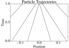
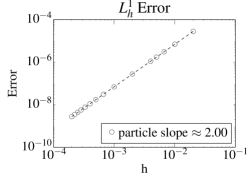
Figure 2. A comparison of exact solutions (solid lines) and particle method solutions (dashed lines). The log-log plot of the error (right) corresponds to $t=0.5$.

Particle method, regular initial data: Figure 2 compares a particle method approximation with an exact solution for initial data (4.3). To compute the particle method approximation, we remove the singularity at zero by setting $\nabla K(0)=0$, instead of regularizing the kernel. Since $K$ is the Newtonian potential, the particle method densities are point masses, which do not belong to $L^{p}_{h}$. Thus, we only consider the particle trajectories defined by this method.

Unlike the blob method solution from in the previous example, the particle method trajectories do not bend away at blowup time. However, a log-log plot of the $L^{1}_{h}$ error reveals a slower rate of convergence than for the blob method, consistent with the rate of $\mathcal{O}(h^{2-\epsilon})$ for particle approximations of the Euler equations [39, 42].

\begin{overpic}[trim=31.2982pt 28.45274pt 14.22636pt 28.45274pt,clip,width=173.44534pt]{D1_Newt_Nx50_Nt200_q9_t1_patch_part.pdf} \put(22.5,66.2){\small A.} \end{overpic}

\begin{overpic}[trim=31.2982pt 28.45274pt 14.22636pt 28.45274pt,clip,width=173.44534pt]{D1_Newt_Nx50_Nt200_q9_t1_patch_den.pdf} \put(36.0,66.2){\small B.} \end{overpic}

\begin{overpic}[trim=31.2982pt 31.2982pt 22.76228pt 28.45274pt,clip,width=173.44534pt]{D1_Newt_Nx50_Nt200_q9_t1_patch_part_zoom.pdf} \put(24.5,66.5){\small C.} \end{overpic}

\begin{overpic}[trim=28.45274pt 30.72902pt 8.5359pt 19.91684pt,clip,width=182.1196pt]{Error_D1_Newt_q9_m4_t5_patch.pdf} \put(38.0,65.0){\small D.} \end{overpic}

Figure 3. A comparison of exact solutions (solid lines) and blob method solutions (dashed lines) with $\delta=h^{q}$ for $q=0.9$. The densities (B) are shown at $t=0,0.4,0.8$. The log-log plot (D) corresponds to $t=0.5$.

Discontinuous initial data: Figure 3 compares exact and blob method solutions to the one dimensional aggregation equation with discontinuous initial data

(4.4) $$\rho_{0}(x)=1_{[-1,1]}(x)=\begin{cases}1&\mbox{if }|x|\leq 1\ ,\\ 0&\mbox{otherwise}\ .\end{cases}$$

Though our convergence results only apply to sufficiently regular solutions to the aggregation equation, the definition of the blob method (Definition 2.2) merely requires that initial data to be a compactly supported function.

We discretize the domain $[-1,1]$ using $h=0.04$. At this level of resolution, the approximate and exact particle trajectories are visually indistinguishable (A), though the approximate density becomes rounded at $t=0.8$ (B), with a similar oscillating profile as the mollifier (4.1).

Considering the particle trajectories on a smaller spatial scale (C), we again observe the trajectories bending away to avoid collision. As expected, a log-log plot of the $L^{1}_{h}$ error (D) reveals a slower rate of convergence than in Figure 1. Unlike in the previous example, for which the slower rate of convergence was due to using a particle method instead of the blob method, in this example the slower rate of convergence is due to the lower regularity of the initial data.

4.3. One dimension, Various potentials

	particle                       $m=4$                       $m=6$
$K(x)=|x|^{3}/3$

Figure 4. A comparison of the $L^{1}_{h}$ error at $t=0.5$ for various kernels and numerical methods. For $K=(-\Delta)^{-1}$, we use analytic expressions for $\nabla K*\psi_{\delta}$ and $\Delta K*\psi_{\delta}$. For the cubic potential, we compute the convolutions using a fast Fourier transform in radial coordinates on a ball of radius 2.5 with $5\times 10^{5}$ grid points (for $m=4$) and $2\times 10^{6}$ grid points (for $m=6$).

Figure 4 compares the rate of convergence of numerical solutions when $K=(-\Delta)^{-1}$ or $K(x)=|x|^{3}/3$. The mollifiers (4.1) are of order $m=4$ and $m=6$. The scaling of the regularization is $\delta=h^{q}$ for $q=0.9$, and the initial data is

(4.5) $$\rho_{0}(x)=\begin{cases}(1-x^{2})^{10}&\mbox{if }|x|\leq 1\ ,\\ 0&\mbox{otherwise}\ .\end{cases}$$

The more singular the kernel, the greater improvement we see in using the blob method over a particle method. For the negative Newtonian potential, the $m=4$ blob method improves upon the particle method, and the $m=6$ blob method shows even greater improvement. For the cubic potential, the particle method is better than the $m=4$ blob method for the trajectories, but not for the density. The $m=6$ blob method is best for both trajectories and density.

For both kernels, the rates of convergence for the $m=4$ blob method are very close to the theoretically predicted rate of $mq=3.6$, while the rates of convergence for the $m=6$ blob method are not as good as the theoretically predicted rate of $mq=5.4$, due to other sources of error in the numerical implementation.

4.4. Two Dimensions

$\rho_{0}(x)=(1-x^{2})_{+}^{2}$		$\rho_{0}(x)=1_{[-1,1]}$
$m=4$	particle	$m=4$

Figure 5. A comparison of $L^{1}_{h}$ error at $t=0.5$ for the two dimensional aggregation equation when $K=(\Delta)^{-1}$.

Newtonian potential: Figure 5 compares the rate of convergence of numerical solutions when $K=(\Delta)^{-1}$ for various choices of initial data. In the first and third plot, the numerical solution is computed via the blob method with a mollifier (4.2) of order $m=4$ and $\delta=h^{q}$ for $q=0.9$. In the second plot, the numerical solution is computed via a particle method.

As in the one dimensional case, we see the best rates of convergence for the blob method applied to regular initial data (left). This agrees with our theoretically predicted rate of $mq=3.6$. The rates of convergence for a particle method applied to regular initial data (middle) and the blob method applied to discontinuous initial data (right) are slower.

	$K(x)=\log|x|/2\pi\hskip 48.36958ptK(x)=|x|^{2}/2\hskip 56.9055ptK(x)=|x|^{3}/3$
regular initial data
discontinuous initial data

Figure 6. A comparison of blob method solutions for the two dimensional aggregation equation. The scaling of the regularization is $\delta=h^{q}$ for $q=0.9$, and the mollifier (4.2) satisfies $m=4$. In the top six plots, the unit square is discretized using $h\approx 0.13$. In the bottom six plots, the unit square is discretized using $h\approx 0.07$.

Newtonian, quadratic, and cubic potentials: Figure 6 illustrates various phenomena of blob method solutions for three choices of kernel (Newtonian, quadratic, and cubic) as well as two choices of initial data (regular and discontinuous).

The top six plots illustrate the behavior of solutions with smooth, compactly supported initial data,

$$\rho_{0}(x)=\begin{cases}e^{1/(x^{2}-1)}&\mbox{if }|x|\leq 1\ ,\\ 0&\mbox{otherwise}\ .\end{cases}$$

The first row shows the space-time trajectories of twenty particles, and the second row shows the density at time $t=1.4$. For $K=(\Delta)^{-1}$, finite time blowup of the classical solution occurs at $t=1/\rho_{0}(0)\approx 1.2$, and the particle trajectories become very close at this time, bending to avoid collision. Two subsequent near-collisions occur before $t=3.2$. For $K(x)=|x|^{2}/2$, the particles converge to a point in infinite time, while for $K(x)=|x|^{3}/3$, the particles converge to a ring in infinite time. Each of these phenomena is reflected in the evolution of the density.

The second two rows consider discontinuous initial data given by the characteristic function on a star shaped patch,

(4.6) $$\rho_{0}(r,\theta)=\begin{cases}1&\mbox{if }r<\left(\sin^{2}(\frac{5\theta}{2})+\frac{1}{2}\right)/4\ ,\\ 0&\mbox{otherwise}\ .\end{cases}$$

All six plots show the approximate density at $t=0.8$, either from the side or above. For $K=(\Delta)^{-1}$, the density exhibits the same rounding due to regularization as in the one dimensional case. For $K(x)=|x|^{2}/2$, there is no rounding due to regularization since convolution with a mollifier of accuracy $m=4$ preserves polynomials of degree less than 4, including $\nabla K$ and $\Delta K$. For $K(x)=|x|^{3}$, the density again converges to a ring in infinite time.

$K(x)=\frac{|x|^{4}}{4}-\frac{\log|x|}{2\pi}$	$K(x)=\frac{|x|^{4}}{4}-\frac{|x|^{3/2}}{3/2}$	$K(x)=\frac{|x|^{7}}{7}-\frac{|x|^{3/2}}{3/2}$

Figure 7. A comparison of numerical solutions to the aggregation equation. The mollifier (4.2) satisfies $m=4$, and the unit square is discretized with $h\approx.11$. For the first kernel, we use an analytic expression for $\nabla K_{\delta}$. For the second two kernels, we numerically compute the convolution $\nabla K*\psi_{\delta}$ in radial coordinates on a ball of radius 2.5 with 100 grid points.

Repulsive-attractive power law kernels: Figure 7 displays the evolution of particle trajectories for numerical solutions to the two dimensional aggregation equation with repulsive-attractive power law kernels. In the past few years, there has been significant interest in such kernels, due to the stationary patters which develop [5, 4, 14, 6, 13, 12, 10, 11, 21, 23, 28, 34, 33, 36, 35, 44, 45, 48, 59, 60, 64, 65, 43].

Figure 7 compares the results of a particle method with the blob method. In all six plots, the initial data is

(4.7) $$\rho_{0}(x)=\begin{cases}C(1-x^{2})^{2}&\mbox{if }|x|\leq 1\ ,\\ 0&\mbox{otherwise}\ ,\end{cases}$$

with $C$ chosen so that $\int\rho_{0}=1$.

For each of the three choices of kernel, the corresponding plots demonstrate that a large regularization parameter—in this case $\delta\approx 0.32$—can affect the steady states of blob method solutions. This effect vanishes as $\delta$ becomes small, but it still of interest since it illustrates the important role of the kernel’s regularity in the dimensionality of steady states. Balagué, Carrillo, Laurent, and Raoul proved that the dimensionality of the support of steady state solutions depends on the strength of the repulsive forces at the origin [4]. For a repulsive-attractive power law kernel,

$$K(x)=|x|^{a}/a-|x|^{b}/b\ ,\quad a>b\ ,$$

the repulsive part is more singular than the attractive part, so regularizing the kernel by convolution with a mollifier has a greater effect for the repulsive part, and we expect this to dampen the repulsive forces.

For $K(x)=|x|^{4}/4-\log|x|/2\pi$, we recover the radial, integrable, compactly supported steady states found by Fetecau, Huang, and Kolokolnikov [36]. A large regularization parameter causes the steady states to collapse to a ring. For $K(x)=|x|^{4}/4-|x|^{3/2}/(3/2)$, we recover the stable delta ring found by Kolokonikov, Sun, Uminsky, and Bertozzi [48]. A comparison of the particle and blob methods at $t=8$ indicates that the blob method solution converges to the ring more quickly. For $K(x)=|x|^{7}/7-|x|^{3/2}/(3/2)$, we recover the ring formation and breakup found by Bertozzi, Sun, Kolokolnikov, Uminsky, and Von Brecht [14]. A large regularization parameter lowers the dimension of the steady state to three point masses.

$K(x)=e^{-|x|}-2e^{-|x|/2}$	$K(x)=2e^{-|x|}-2e^{-|x|/2}$
regular initial data	regular initial data	discontinuous initial data

Figure 8. A comparison of numerical solutions to the aggregation equation computed by particle and blob methods. The mollifier (3.1) is chosen so that $m=4$, and the unit square is discretized with $h\approx 0.11$. The spatial scale in the first column is the unit square, and the spatial scale is doubled in the second and third columns. For all three kernels, we numerically compute the convolution $\nabla K*\psi_{\delta}$ and $\Delta K*\psi_{\delta}$ in radial coordinates on a ball of radius 5 with 200 grid points.

Repulsive-attractive Morse potential: Figure 8 shows the evolution of particle trajectories for numerical solutions to the aggregation equation when the kernel is given by a repulsive-attractive Morse potential, comparing the results of a particle method with the blob method. In the first two columns, the initial data is given by (4.7), with $C$ chosen so that $\int\rho_{0}=1$. In the third column, the initial data is given by a star shaped patch (4.6).

We only observe the effect of a large regularization parameter for the kernel $K(x)=2e^{-|x|}-2e^{-|x|/2}$ with regular initial data. This is likely due to the fact that the repulsive and attractive components of the kernel have the same regularity, so regularization does not disproportionately affect one without the other.

5. Conclusion

We develop a new numerical method for the aggregation equation for a range of kernels, including singular kernels, kernels which grow at infinity, and repulsive-attractive kernels. We prove that our blob method solutions converge to classical solutions of the aggregation equation with arbitrarily high rates of convergence, depending on the choice of blobs. We also provide several numerical examples which confirm our theoretically predicted rates of convergence and illustrate key properties of the method, including long-time existence of particle trajectories.

As analysis of numerical methods for the aggregation equation is a relatively new area of interest, there are several directions for future work. First, our estimates do not differentiate between purely repulsive, purely attractive, or repulsive-attractive kernels, and our numerical method may be improved by leveraging the different dynamics in each of these cases. In particular, a numerical method for repulsive or repulsive-attractive kernels might take advantage of the formation of steady states to obtain global in time bounds on the error. Preliminary analysis in this direction indicates that it will be necessary to measure error in different norms. Our current discrete $L^{p}$ norms measure the distance between exact and approximate solutions along particle trajectories that begin at the same grid point. However, small perturbations of the functional can change where particles settle in a steady state. This causes the discrete $L^{p}_{h}$ norm of the error to be large, even if the overall structure of the steady state is the same.

Another direction for future work is to adapt the blob method to the Keller-Segel equation by the addition of (possibly degenerate) diffusion. From the perspective of classical vortex methods, the addition of diffusion corresponds to passing from the Euler equations to the Navier Stokes equations, so it may be possible to adapt random vortex or core spreading methods from the Navier Stokes equations to the Keller-Segel equation [62, 25, 52, 38, 50]. Our method might also be extended to the Keller-Segel equation by separately simulating the effects of aggregation and (degenerate) diffusion at each time step. Yao and Bertozzi developed such a method by using a radial particle method to simulate aggregation and an implicit finite volume scheme to simulate degenerate diffusion [69]. The blob method would allow one to perform the aggregation step for non-radial solutions with a high degree of accuracy.

Finally, our result on the convergence of the blob method to classical solutions might be extended to weak measure solutions. Lin and Zhang [49] used a blob method to prove existence of weak measure solutions for the two dimensional aggregation equation when $K=(-\Delta)^{-1}$. The blob method might also be used to prove existence of weak measure solutions for the multidimensional aggregation equation for a range of singular kernels. This would build on the work of Bertozzi, Garnett, and Laurent for radial initial data and kernels of the form $K(x)=|x|^{a}$, $2-d\leq a<2$ [12]. Such a result would be of particular interest for kernels in the range $K(x)=|x|^{-1}$ to $K(x)=|x|$, for which uniqueness may also hold.

6. Appendix

6.1. Discrete $L^{p}$ and Sobolev Norms

In this section, we provide references and proofs for the discrete norm inequalities given in Proposition 3.1. We begin with the following lemma regarding extensions for discrete Sobolev spaces.

Lemma 6.1 (extensions from $W^{1,p}_{h}(Q_{R})$ to $W^{1,p}_{h}({\mathord{\mathbb{R}}^{d}})$).

Let $Q_{R}=[-R,R]^{d}$ for $R\geq 3$. For all $0<h<1$, there exists $P:W^{1,p}_{h}(Q_{R})\to W^{1,p}_{h}({\mathord{\mathbb{R}}^{d}})$ satisfying $Pg|_{Q_{R}}=g$ and $\|Pg\|_{W^{1,p}_{h}({\mathord{\mathbb{R}}^{d}})}\leq C_{d,p}\|g\|_{W^{1,p}_{h}(Q_{R})}$.

Proof.

Denote the vertices of $Q_{R}$ by $\vec{v}\in\{(v_{1},\dots,v_{d}):v_{i}=\pm R\}$. Define a partition of unity $\{\eta_{\vec{v}}\}$ on $Q_{R}$ so that $0\leq\eta_{\vec{v}}\leq 1$, $\sum_{\vec{v}}\eta_{\vec{v}}=1$, and $\eta_{\vec{v}}(x)$ vanishes on the edges of the cube opposite $\vec{v}$, i.e. whenever $x=(x_{1},\dots,x_{d})$ satisfies $|x_{j}-(-v_{j})|<1$.

For any $g\in W^{1,p}_{h}(Q_{R})$, define $g_{\vec{v}}=\eta_{\vec{v}}g$. We claim that for all $g_{\vec{v}}$, there exists an extension $Pg_{\vec{v}}$ so that $Pg_{\vec{v}}|_{Q_{R}}=g_{\vec{v}}$ and $\|Pg_{\vec{v}}\|_{W^{1,p}_{h}({\mathord{\mathbb{R}}^{d}})}\leq C_{d,p}\|g_{\vec{v}}\|_{W^{1,p}_{h}(Q_{R})}$. Supposing this claim holds, define the extension $Pg$ of $g$ by $Pg=\sum_{\vec{v}}Pg_{\vec{v}}$. This satisfies $Pg|_{Q_{R}}=\sum_{\vec{v}}Pg_{\vec{v}}|_{Q_{R}}=\sum_{\vec{v}}g_{\vec{v}}=g$ and

$$\|Pg\|_{W^{1,p}_{h}({\mathord{\mathbb{R}}^{d}})}\leq\sum_{\vec{v}}\|Pg_{\vec{v}}\|_{W^{1,p}_{h}({\mathord{\mathbb{R}}^{d}})}\leq\sum_{\vec{v}}C_{d,p}\|g_{\vec{v}}\|_{W^{1,p}_{h}(Q_{R})}\leq C_{d,p}\|g\|_{W^{1,p}_{h}(Q_{R})}\ .$$

Thus it remains to construct the extension $Pg_{\vec{v}}$. By translation invariance, we suppose that $Q_{R}=[0,2R]^{d}$, and by rotational symmetry, we suppose that $\vec{v}=(0,0,\dots,0)$. Then $g_{\vec{v}}\in W^{1,p}(Q_{R})$ and $g_{\vec{v}}(x)=0$ whenever $x=(x_{1},\dots,x_{d})$ satisfies $|x_{j}-2R|<1$. To extend $g_{\vec{v}}$ to all of ${\mathord{\mathbb{R}}^{d}}$, first reflect the function across each coordinate axis, giving a function defined on $[-2R,2R]^{d}$, and then extend it to be zero outside of $[-2R,2R]^{d}$. The resulting extension satisfies $Pg_{\vec{v}}|_{Q_{R}}=g_{\vec{v}}$ and $\|Pg_{\vec{v}}\|_{W^{1,p}_{h}({\mathord{\mathbb{R}}^{d}})}\leq C_{d,p}\|g_{\vec{v}}\|_{W^{1,p}_{h}(Q_{R})}$. ∎

We now turn to the proof of Proposition 3.1.

Proof of Proposition 3.1.

1. The result follows from Hölder’s inequality on $\ell^{p}$ and the definition of $W^{-1,p}_{h}$.

   $$\|u\|_{W^{-1,p}_{h}}=\sup_{g\in W^{1,p^{\prime}}_{h}}\frac{|(u,g)_{h}|}{\|g\|_{W^{1,p^{\prime}}_{h}}}\leq\sup_{g\in W^{1,p^{\prime}}_{h}}\frac{\|u\|_{L^{p}_{h}}\|g\|_{L^{p^{\prime}}_{h}}}{\|g\|_{W^{1,p^{\prime}}_{h}}}\leq\|u\|_{L^{p}_{h}}$$

   (See also [7, Equation 2.9].)

2. By definition of the ${W^{-1,p}_{h}}$ norm,

   (6.1) $$|(u,g)_{h}|\leq\|u\|_{W^{-1,p}_{h}}\|g\|_{W^{1,p^{\prime}}_{h}}\leq(1+2d/h)\|u\|_{W^{-1,p}_{h}}\|g\|_{L^{p^{\prime}}_{h}}\ .$$

   Suppose $p<+\infty$. If we define $g=\{|u_{i}|^{p-2}u_{i}\}$ and use that $(p-1)p^{\prime}=p$,

   $$(u,g)_{h}=\sum|u_{i}|^{p}h^{d}=\|u\|_{L^{p}_{h}}^{p}\ \text{ and }\ \|g\|_{L^{p^{\prime}}_{h}}^{p^{\prime}}=\sum|u_{i}|^{(p-1)p^{\prime}}h^{d}=\|u\|_{L^{p}_{h}}^{p}\ .$$

   Thus, $\|u\|_{L^{p}_{h}}\leq(1+2d/h)\|u\|_{W^{-1,p}_{h}}$.

   If $p=+\infty$, define $g^{j}_{i}$ to be $1$ if $i=j$ and $0$ otherwise. Then (6.1) implies

   $$|u_{j}|h^{d}\leq(1+2/h)\|u\|_{W^{-1,\infty}_{h}}h^{d}\ ,$$

   so $\|u\|_{L^{\infty}_{h}}\leq(1+2d/h)\|u\|_{W^{-1,\infty}_{h}}$. (See also [7, Equation 2.10].)

3. If $\Omega\subseteq B_{R}$, the number of grid points in $\Omega$ is bounded by $C_{R}h^{-d}$. By an elementary inequality for $\ell^{p}$ norms on finite dimensional vector spaces,

   $$\|u\|_{L^{q}_{h}(\Omega)}=h^{d/q}\|u\|_{\ell^{q}}\leq(C_{R}h^{-d})^{\frac{1}{q}-\frac{1}{p}}h^{d/q}\|u\|_{\ell^{p}}\leq C_{R,q,p}\|u\|_{L^{p}_{h}(\Omega)}\ .$$

4. Fix $Q_{R}=[-R,R]^{d}$, so by $(c)$,$\|g\|_{W^{1,p^{\prime}}_{h}(Q_{R})}\leq C_{p,q,R}\|g\|_{W^{1,q^{\prime}}_{h}(Q_{R})}\leq C_{p,q,R}\|g\|_{W^{1,q^{\prime}}_{h}}$. By Lemma 6.1, there exists an extension operator $P:W^{1,p^{\prime}}_{h}(Q_{R})\to W^{1,p^{\prime}}_{h}({\mathord{\mathbb{R}}^{d}})$. Since $u$ is supported in $B_{R}\subseteq Q_{R}$,

   $$|(u,g)_{h}| =|(u,Pg)_{h}|\leq\|u\|_{W^{-1,p}_{h}}\|Pg\|_{W^{1,p^{\prime}}}\leq\|u\|_{W^{-1,p}_{h}}\|g\|_{W^{1,p^{\prime}}_{h}(Q_{R})}$$

   $$\leq C_{p,q,R}\|u\|_{W^{-1,p}_{h}}\|g\|_{W^{1,q^{\prime}}_{h}}\ .$$

5. See [8, Proposition 2.1].

∎

6.2. Proof of Regularity of Velocity Field and Particle Trajectories

In this section we prove Lemma 3.6 on the regularity of the velocity field $\vec{v}=\nabla K*\rho$, the divergence of the velocity field $\nabla\cdot\vec{v}=\Delta K*\rho$ and Lemma 3.7 on the regularity of the particle trajectories $X^{t}(\alpha)$ and the Jacobian determinants $J^{t}(\alpha)$.

Proof of Lemma 3.6.

By the linearity of differentiation and convolution, it is enough to show the result in the specific case that that $K=K_{1}$ with $s=S\geq 1-d$.

When $s=1-d$, $K$ is a constant multiple of the Newtonian potential. By Assumption 3.5, $\rho\in C^{1}([0,T],C^{r}_{c}({\mathord{\mathbb{R}}^{d}}))$ for $r\geq m,L$ and has compact support. It is a classical result that $\Delta K*\rho=C\rho$. Thus $\nabla\cdot\vec{v}=\Delta K*\rho$ belongs to $C^{L}({\mathord{\mathbb{R}}^{d}})\cap C^{m}({\mathord{\mathbb{R}}^{d}})$ and has bounded derivatives up to order $m$.

Now, we may assume that both $\nabla K$ and $\Delta K$ are homogeneous of order at least $1-d$. We treat both simultaneously by proving the result for a kernel $\mathcal{K}$, which for fixed $l\geq 1-d$ satisfies

$$|\partial^{\beta}\mathcal{K}(x)|\leq C|x|^{l-|\beta|},\ \forall x\in{\mathord{\mathbb{R}}^{d}}\setminus\{0\},0\leq|\beta|\leq l+d-1\ .$$

Note that this implies $\partial^{\beta}\mathcal{K}\in L^{1}_{\rm loc}({\mathord{\mathbb{R}}^{d}})$ for all $|\beta|\leq l+d-1$. When $\mathcal{K}(x)=\nabla K(x)$, $l=s$, and when $\mathcal{K}(x)=\Delta K(x)$, $l=s-1$. The fact that $\mathcal{K}*\rho\in C^{L}({\mathord{\mathbb{R}}^{d}})$ is immediate, since $\rho\in C^{L}_{c}({\mathord{\mathbb{R}}^{d}})$ and $\mathcal{K}\in L^{1}_{\rm loc}({\mathord{\mathbb{R}}^{d}})$. We now turn to the estimates that imply $\mathcal{K}*\rho\in C^{m}({\mathord{\mathbb{R}}^{d}})$ and the bound on its derivatives.

We prove by induction that for ${0\leq|\gamma|\leq l+d-1}$,

$$\partial^{\gamma}\mathcal{K}*\rho(x)=\int\partial^{\gamma}\mathcal{K}(x-y)\rho(y)dy\ .$$

If $|\gamma|=0$, equality holds. Suppose $|\gamma|\geq 1$ and $\partial^{\beta}\mathcal{K}*\rho(x)=\int\partial^{\beta}\mathcal{K}(x-y)\rho(y)dy$ for all $|\beta|=|\gamma|-1$. If $|\eta|=1$ satisfies $\partial^{\eta}\partial^{\beta}=\partial^{\gamma}$,

$$\partial^{\gamma}(K*\rho)=\partial^{\eta}((\partial^{\beta}\mathcal{K})*\rho)=(\partial^{\beta}\mathcal{K})*(\partial^{\eta}\rho)\ .$$

We now move $\partial^{\eta}$ onto $\mathcal{K}$. Fixing $\epsilon\in(0,1)$,

$$(\partial^{\beta}\mathcal{K})*(\partial^{\eta}\rho)(x) =\int_{|y|<\epsilon}\partial^{\beta}\mathcal{K}(y)\partial^{\eta}_{x}\rho(x-y)dy+\int_{|y|\geq\epsilon}\partial^{\beta}\mathcal{K}(y)\partial^{\eta}_{x}\rho(x-y)dy$$

$$=\mathcal{O}(\epsilon^{d+l-|\beta|})+\int_{|y|\geq\epsilon}\partial^{\gamma}\mathcal{K}(y)\rho(x-y)dy+\mathcal{O}(\epsilon^{d-1+l-|\beta|})\ .$$

Since $|\beta|=|\gamma|-1\leq l+d-2$, sending $\epsilon\to 0$ gives

$$(\partial^{\beta}\mathcal{K})*(\partial^{\eta}\rho)(x)=(\partial^{\gamma}\mathcal{K})*\rho(x)\ .$$

This shows $\mathcal{K}*\rho\in C^{l+d-1}({\mathord{\mathbb{R}}^{d}})$. We now show $\mathcal{K}*\rho\in C^{m}({\mathord{\mathbb{R}}^{d}})$. If $m\leq l+d-1$, this is immediate, so suppose $m>l+d-1$. By Assumption 3.5, $\rho\in C^{r}_{c}({\mathord{\mathbb{R}}^{d}})$ for $r\geq m-(s+d-2)$. Since $\partial^{\gamma}(\mathcal{K}*\rho)=(\partial^{\gamma}\mathcal{K})*\rho$ and $\partial^{\gamma}\mathcal{K}\in L^{1}_{\rm loc}$ for all $|\gamma|\leq l+d-1$, for any $|\beta|=m$, there exists $|\eta|=m-(l+d-1)\leq r$ so that

$$\partial^{\beta}\mathcal{K}*\rho=(\partial^{\gamma}\mathcal{K})*(\partial^{\eta}\rho)\ .$$

Thus, $\mathcal{K}*\rho\in C^{m}({\mathord{\mathbb{R}}^{d}})$.

Finally, we show that $|\partial^{\beta}\mathcal{K}*\rho(x,t)|\leq C(1+|x|^{(l-|\beta|)_{+}})$ for $|\beta|\leq m$. If ${|\beta|\geq l+d-1}$, let $|\eta|=|\beta|-(l+d-1)$ and $|\gamma|=l+d-1$ so that $\partial^{\beta}=\partial^{\eta}\partial^{\gamma}$. Otherwise, let $\gamma=\beta$ and $\eta=0$. Since $\partial^{\beta}\mathcal{K}*\rho(x)$ is continuous, it is bounded for $|x|\leq 2R_{0}$. If $|x|>2R_{0}$,

$$|\partial^{\beta}\mathcal{K}*\rho(x)| =|(\partial^{\gamma}\mathcal{K})*(\partial^{\eta}\rho)(x)|\leq C\int|x-y|^{l-\gamma}|\partial^{\eta}\rho(y)|dy\leq C\int_{B_{R_{0}}}|x-y|^{l-\gamma}dy$$

$$\leq\begin{cases}C|x|^{l-\gamma}&\text{ if }l>\gamma\ ,\\ C&\text{ if }l\leq\gamma\ .\end{cases}$$

Thus, $|\partial^{\beta}\mathcal{K}*\rho(x)|\leq C(1+|x|^{(l-|\beta|)_{+}})$. The constant depends on the exact solution, the kernel, the dimension, $\beta$, $T$, and $R_{0}$. ∎

We now prove Lemma 3.7 on the regularity of the particle trajectories.

Proof of Lemma 3.7.

Assumption 3.5 and Lemma 3.6 ensure sufficient regularity on the velocity field so that there exists a time interval $[0,T_{0}]$ on which, for $\alpha\in B_{R_{0}+2}$, the particle trajectories $X^{t}(\alpha)$ and their inverses $X^{-t}(\alpha)$ uniquely exist, are continuously differentiable in time, and $C^{L}$ in space. Likewise $J^{t}(\alpha)$ and $J^{-t}(\alpha)$ are $C^{L-1}$ in space and satisfy equation (3.2) .

Suppose $T_{0}<T$. Then there exists $\alpha$ so that $|X^{t}(\alpha)|\to+\infty$ as $t\to T_{0}$. This contradicts Assumption 3.5. Therefore, $T_{0}=T$.

If $s=1-d$, we may replace $B_{R_{0}+2}$ with ${\mathord{\mathbb{R}}^{d}}$. ∎

6.3. Proof of Regularized Kernel Estimates

We now prove the regularized kernel estimates from Section 3. Throughout, we use that

(6.2) $$\begin{cases}|y|^{s}\in L^{1}(B_{1}(0))\text{ and }|y|^{s}\in L^{\infty}({\mathord{\mathbb{R}}^{d}}\setminus B_{1}(0))&\text{ if }1-d\leq s\leq 0\ ,\\ |y|^{s}\in L^{\infty}(B_{1}(0))&\text{ if }0<s\ .\end{cases}$$

Proof of Lemma 3.15.

By the linearity of differentiation and convolution, it is enough to show the result in the specific case that that $K=K_{1}$ with $s=S\geq 1-d$.

If $s=1-d$, $K$ is a constant multiple of the Newtonian potential. In this case, since $\psi\in C^{L}({\mathord{\mathbb{R}}^{d}})$ for $L\geq d+2$, it is a classical result that $\Delta K_{\delta}=\Delta K*\psi_{\delta}=C\psi_{\delta}$. Assumption 3.3 ensures $\psi_{\delta}\in C^{L}({\mathord{\mathbb{R}}^{d}})$, hence $\Delta K_{\delta}\in C^{L}({\mathord{\mathbb{R}}^{d}})$.

We may now treat the cases of $\nabla K_{\delta}$ and $\Delta K_{\delta}$ simultaneously by proving the result for a kernel $\mathcal{K}_{\delta}=\mathcal{K}*\psi_{\delta}$, which for fixed $l\geq 1-d$ satisfies

$$|\partial^{\beta}\mathcal{K}(x)|\leq C|x|^{l-|\beta|},\ \forall x\in{\mathord{\mathbb{R}}^{d}}\setminus\{0\},0\leq|\beta|\leq l+d-1\ .$$

When $\mathcal{K}(x)=\nabla K(x)$, $l=s$ and when $\mathcal{K}(x)=\Delta K(x)$, $l=s-1$.

It is enough to show that in a neighborhood around every $x$, there exists $g(y)\in L^{1}({\mathord{\mathbb{R}}^{d}})$ which dominates $\mathcal{K}(y)\partial^{\beta}_{x}\psi_{\delta}(x-y)$. Then, the mean value theorem ensures that the difference quotient which converges to this derivative at $x$ is also dominated by $g(y)$, allowing us to conclude

$$\partial^{\beta}\int\mathcal{K}(y)\psi_{\delta}(x-y)dy=\int\mathcal{K}(y)\partial^{\beta}\psi_{\delta}(x-y)dy\ ,$$

and $\mathcal{K}_{\delta}\in C^{L}({\mathord{\mathbb{R}}^{d}})$. We use Assumption 3.3 on the decay and regularity of $\psi$ to find dominating functions when $l\leq 0$ and $l>0$.

If $1-d\leq l\leq 0$, the decay and regularity assumptions ensure that there exists $\epsilon>0$ so that $|\partial^{\beta}\psi(x)|\leq C|x|^{-d-\epsilon}$ for all $|\beta|\leq L$. If $l>0$ the regularity assumption ensures that $|\partial^{\beta}\psi(x)|\leq C|x|^{-d-l-\epsilon}$ for all $|\beta|\leq L$. Since $\partial^{\beta}\psi$ is bounded near the origin, there exists $C^{\prime}>0$ so that for all $x\in{\mathord{\mathbb{R}}^{d}}$,

$$|\partial^{\beta}\psi(x)|\leq\begin{cases}C^{\prime}(|x|+1)^{-d-\epsilon}&\text{ if }1-d\leq l\leq 0\ ,\\ C^{\prime}(|x|+1)^{-d-\epsilon-l}&\text{ if }0<l\ .\end{cases}$$

Therefore,

(6.3) $$|\mathcal{K}(y)\partial^{\beta}\psi_{\delta}(x-y)|\leq\begin{cases}C_{\delta}|y|^{l}(|x-y|+1)^{-d-\epsilon}&\text{ if }1-d\leq l\leq 0\ ,\\ C_{\delta}|y|^{l}(|x-y|+1)^{-d-\epsilon-l}&\text{ if }0<l\ .\end{cases}$$

If $|x|<R$ and $|y|>2R$, $|x-y|+1>|y|-|x|>\frac{1}{2}|y|$. This gives the following dominating functions when $|x|<R$:

$$|\mathcal{K}(y)\partial^{\beta}\psi_{\delta}(x-y)|\leq\begin{cases}C_{\delta,R}|y|^{l}1_{|y|\leq 2R}+C_{\delta,R}1_{|y|>2R}&\text{ if }1-d\leq l\leq 0\ ,\\ C_{\delta,R}&\text{ if }0<l\ .\end{cases}$$

Since $R$ was arbitrary, $\partial^{\beta}\mathcal{K}_{\delta}(x)=\mathcal{K}*\partial^{\beta}\psi_{\delta}(x)$ for all $x\in{\mathord{\mathbb{R}}^{d}}$. ∎

Proof of Lemma 3.16.

Our proof generalizes the approaches of Beale and Majda [8] and Anderson and Greengard [3]. By the linearity of differentiation and convolution, it is enough to show the result in the specific case that that $K=K_{1}$ with $s=S\geq 1-d$.

We first prove the following pointwise bounds for $|\beta|\leq L$ and $r>0$:

$$|\partial^{\beta}\nabla K_{\delta}(x)|\leq\begin{cases}C|x|^{s-|\beta|}&\mbox{if }\delta\leq|x|\ ,\\ C\delta^{s-|\beta|}&\mbox{if }|x|\leq r\delta\ .\end{cases}$$

We begin with $|x|\leq r\delta$. By Lemma 3.15, $\partial^{\beta}\nabla K_{\delta}=\nabla K*(\partial^{\beta}\psi_{\delta})$, so

$$|\partial^{\beta}\nabla K_{\delta}(x)| \leq\int|\nabla K(y)||\partial^{\beta}\psi_{\delta}(x-y)|dy\leq C\int|y|^{s}\delta^{-d-|\beta|}\left|\partial^{\beta}\psi\left(\frac{x-y}{\delta}\right)\right|dy\ ,$$

(6.4) $$\leq C\int|\delta y|^{s}\delta^{-|\beta|}\left|\partial^{\beta}\psi\left(\frac{x}{\delta}-y\right)\right|dy=C\delta^{s-|\beta|}\int|y|^{s}\left|\partial^{\beta}\psi\left(\frac{x}{\delta}-y\right)\right|dy\ .$$

Suppose $1-d\leq s\leq 0$. By (6.2),

$$|\partial^{\beta}\nabla K_{\delta}(x)|\leq C\delta^{s-|\beta|}\left\{\|\partial^{\beta}\psi\|_{L^{\infty}({\mathord{\mathbb{R}}^{d}})}\int_{|y|\leq 1}|y|^{s}dy+\sup_{|y|\geq 1}|y|^{s}\ \|\partial^{\beta}\psi\|_{L^{1}}\right\}\leq C\delta^{s-|\beta|}\ .$$

If $s>0$, we apply Assumption 3.3, $|x|\leq r\delta$, and (6.4) to conclude

$$|\partial^{\beta}\nabla K_{\delta}(x)| \leq C\delta^{s-|\beta|}\int\left|y+\frac{x}{\delta}\right|^{s}\left|\partial^{\beta}\psi\left(y\right)\right|dy\ ,$$

$$\leq C\delta^{s-|\beta|}\int\left(|y|+r\right)^{s}\left|\partial^{\beta}\psi\left(y\right)\right|dy\leq C\delta^{s-|\beta|}\ .$$

We now consider the the pointwise estimate on $|\partial^{\beta}K_{\delta}(x)|$ for $|x|\geq\delta$. First suppose $1-d\leq s\leq 0$. Let $\phi_{0}:{\mathord{\mathbb{R}}}\to[0,1]$ satisfy $\phi_{0}(s)=0$ for $s\leq 1/4$ and $\phi_{0}(s)=1$ for $s\geq 1/2$. Define $\phi_{x}(y)=\phi_{0}(|y|/|x|)$. By Lemma 3.15,

$$|\partial^{\beta}\nabla K_{\delta}(x)| =\left|\int\nabla K(y)\partial^{\beta}\psi_{\delta}(x-y)dy\right|\ ,$$

$$\leq\left|\int\nabla K(y)\phi_{x}(y)\partial^{\beta}\psi_{\delta}(x-y)dy\right|+\left|\int\nabla K(y)(1-\phi_{x}(y))\partial^{\beta}\psi_{\delta}(x-y)dy\right|\ ,$$

$$=I_{1}+I_{2}\ .$$

To control $I_{1}$, we integrate by parts,

$$I_{1}\leq\left|\int\partial^{\beta}_{y}(\nabla K(y)\phi_{x}(y))\psi_{\delta}(x-y)dy\right|\ .$$

As $\phi_{x}(y)$ is only nonzero for $|y|/|x|>1/4$, we only need to bound $I_{1}$ for $\delta\leq|x|<4|y|$. For any multiindex $\gamma$, $|\partial_{y}^{\gamma}\phi_{x}(y)|\leq C|x|^{-|\gamma|}$ and by Assumption 3.2, $|\partial^{\gamma}\nabla K(y)|\leq C|y|^{s-|\gamma|}\leq C|x|^{s-|\gamma|}$ for $|x|<4|y|$. Combining these facts with the product rule gives $|\partial^{\beta}_{y}(\nabla K(y)\phi_{x}(y))|\leq C|x|^{s-|\beta|}$. Since $\psi_{\delta}\in L^{1}({\mathord{\mathbb{R}}^{d}})$, this shows

$$I_{1}\leq C|x|^{s-|\beta|}\ .$$

We now turn to $I_{2}$. Since $1-\phi_{x}(y)$ is nonzero for $|y|/|x|<1/2$, and ${|1-\phi_{x}(y)|\leq 1}$,

$$I_{2}\leq\left|\int_{|y|\leq|x|/2}\nabla K(y)\partial^{\beta}\psi_{\delta}(x-y)dy\right|\ .$$

For $y$ in this range, $|x-y|\geq|x|-|y|\geq|x|/2$. By Assumption 3.3 on the regularity of the mollifier, $|x|^{d+|\beta|}|\partial^{\beta}\psi(x)|\leq C$. Therefore,

$$|\partial^{\beta}\psi_{\delta}(x-y)|=\delta^{-d-|\beta|}\left|\partial^{\beta}\psi\left(\frac{x-y}{\delta}\right)\right|\leq C\delta^{-d-|\beta|}|(x-y)/\delta|^{-d-|\beta|}\leq C|x|^{-d-|\beta|}\ .$$

Furthermore, since $s\geq 1-d$,

$$I_{2}\leq C|x|^{-d-|\beta|}\left|\int_{|y|\leq|x|/2}\nabla K(y)dy\right|\leq C|x|^{-d-|\beta|}\int_{0}^{|x|/2}r^{s}r^{d-1}dr\leq C|x|^{s-|\beta|}\ .$$

This completes the proof of the pointwise bounds for $1-d\leq s\leq 0$.

Now we prove the pointwise estimate on $|\partial^{\beta}K_{\delta}(x)|$ for $\delta\leq|x|$ when $s>0$. First, note that for any multiindex $\gamma$ such that $|\gamma|\leq|\beta|$ and $s-|\gamma|\geq-1$,

$$|\partial^{\beta}\nabla K_{\delta}(x)|$$

$$\quad\leq\left|\int_{|y|>\epsilon}\nabla K(x-y)\partial^{\beta}\psi_{\delta}(y)dy\right|+\left|\int_{|y|\leq\epsilon}\nabla K(x-y)\partial^{\beta}\psi_{\delta}(y)dy\right|$$

$$\quad\leq\left|\int_{|y|>\epsilon}\partial^{\gamma}\nabla K(y)\partial^{\beta-\gamma}\psi_{\delta}(x-y)dy\right|+C_{\delta}\sum_{m=0}^{|\gamma|-1}\left|\int_{|y|=\epsilon}|y|^{s-m}dy\right|+C_{\delta}\left|\int_{|y|\leq\epsilon}|y|^{s}dy\right|$$

$$\xrightarrow{\epsilon\to 0}\left|\int\partial^{\gamma}\nabla K(y)\partial^{\beta-\gamma}\psi_{\delta}(x-y)dy\right|$$

If there is some $|\gamma|\leq|\beta|$ so that $s-|\gamma|\leq 0$, then applying the previous argument for $s\leq 0$ to $|\partial^{\gamma}\nabla K|\leq C|x|^{s-|\gamma|}$,

$$|\nabla^{\beta}K_{\delta}(x)|\leq|(\partial^{\gamma}\nabla K)*(\partial^{\beta-\gamma}\psi_{\delta})(x)|\leq C|x|^{-1-(|\beta|-|\gamma|)}=C|x|^{|\gamma|-1-|\beta|}=C|x|^{s-|\beta|}\ .$$

On the other hand, if $s-|\beta|>0$, integrating by parts $|\beta|$ times and applying Assumption 3.3 on the decay of the mollifier when $s>0$ leaves us with

$$|\partial^{\beta}\nabla K_{\delta}(x)| =\left|\int\partial^{\beta}\nabla K(y)\psi_{\delta}(x-y)dy\right|\leq C\int|y|^{s-|\beta|}|\psi_{\delta}(x-y)|dy$$

$$\leq C\int_{|y|\leq 2|x|}|y|^{s-|\beta|}|\psi_{\delta}(x-y)|dy+C\delta^{-d}\int_{|y|>2|x|}|y|^{s-|\beta|}\frac{\delta^{d+s+\epsilon}}{|x-y|^{d+s+\epsilon}}dy$$

The first term is bounded by $C|x|^{s-|\beta|}$. The second term is bounded for $|x|\geq\delta$ by

$$C\delta^{s+\epsilon}\int_{|y|>2|x|}|y|^{s-|\beta|}\frac{1}{(|y|-|x|)^{d+s+\epsilon}}dy\leq C\delta^{s+\epsilon}\int_{|y|>2|x|}|y|^{s-|\beta|}\frac{1}{|y|^{d+s+\epsilon}}dy$$

$$\leq C\delta^{s+\epsilon}\int_{2|x|}^{\infty}r^{-|\beta|-d-\epsilon}r^{d-1}dr\leq C\delta^{s+\epsilon}|x|^{-|\beta|-\epsilon}\leq C|x|^{s-|\beta|}\ .$$

This completes the proof of the pointwise estimates.

Finally, we apply the pointwise estimates to obtain Lemma 3.16. We define $\delta^{\prime}=(C^{\prime}+1)\delta$, and without loss of generality, we assume $R\geq\delta^{\prime}$. First, decompose the integral as

$$\int_{B_{R}}|\partial^{\beta}\nabla K_{\delta}(x+g(x))|dx$$

$$\quad\leq\int_{B_{R}\cap B_{\delta^{\prime}}}|\partial^{\beta}\nabla K_{\delta}(x+g(x))|dx+\int_{B_{R}\setminus B_{\delta^{\prime}}}|\partial^{\beta}\nabla K_{\delta}(x+g(x))|dx$$

$$\quad=I_{3}+I_{4}$$

When $|x|\leq\delta^{\prime}$, $|x+g(x)|\leq 2\delta^{\prime}=2(C^{\prime}+1)\delta$ and $I_{3}\leq C\delta^{s-|\beta|}\delta^{d}\leq C\delta^{s+d-|\beta|}$. When $|x|>\delta^{\prime}$, we use that $|x+g(x)|\geq\delta^{\prime}-C^{\prime}\delta=\delta$ to conclude

$$I_{4} \leq C\int_{B_{R}\setminus B_{\delta^{\prime}}}|x+g(x)|^{s-|\beta|}dx\ .$$

If $s-|\beta|>0$, the fact that $|x+g(x)|\leq 2R$ implies the integral is bounded by a constant which depends on $R$. If $s-|\beta|\leq 0$,

$$I_{4} \leq C\int_{B_{R}\setminus B_{\delta^{\prime}}}(|x|-|g(x)|)^{s-|\beta|}dx\leq C\int_{\delta^{\prime}}^{R}(r-C^{\prime}\delta)^{s-|\beta|}r^{d-1}dr$$

$$\leq C\int_{\delta}^{R-C^{\prime}\delta}r^{s-|\beta|}(r+C^{\prime}\delta)^{d-1}dr\leq C\int_{\delta}^{R}r^{s+d-|\beta|-1}(1+C^{\prime})^{d-1}dr$$

$$\leq\left\{\begin{aligned} &C(R^{s+d-|\beta|}-\delta^{s+d-|\beta|})&&\leq C&\quad\mbox{if }s+d>|\beta|\ ,\\ &C(\log(R)-\log(\delta))&&\leq C|\log\delta|&\quad\mbox{if }s+d=|\beta|\ ,\\ &C(\delta^{s+d-|\beta|}-R^{s+d-|\beta|})&&\leq C\delta^{s+d-|\beta|}&\quad\mbox{if }s+d<|\beta|\ .\end{aligned}\right.$$

The constant depends on the kernel, mollifier, dimension, $\beta$, and $R$. ∎

Acknowledgements: The authors would like to thank MSRI, where part of this work was completed. The authors would also like to thank Prof. José Carrillo and Prof. Jeff Eldredge for very helpful conversations.

References

- [1] Luigi Ambrosio, Nicola Gigli, and Giuseppe Savaré, Gradient flows in metric spaces and in the space of probability measures, second ed., Lectures in Mathematics ETH Zürich, Birkhäuser Verlag, Basel, 2008. MR 2401600 (2009h:49002)
- [2] Luigi Ambrosio and Sylvia Serfaty, A gradient flow approach to an evolution problem arising in superconductivity, Comm. Pure Appl. Math. 61 (2008), no. 11, 1495–1539. MR 2444374 (2010b:35196)
- [3] Christopher Anderson and Claude Greengard, On vortex methods, SIAM J. Numer. Anal. 22 (1985), no. 3, 413–440. MR 787568 (86j:76016)
- [4] D. Balagué, J. A. Carrillo, T. Laurent, and G. Raoul, Dimensionality of local minimizers of the interaction energy, Arch. Ration. Mech. Anal. 209 (2013), no. 3, 1055–1088. MR 3067832
- [5] Daniel Balagué, José Carrillo, Thomas Laurent, and Gaël Raoul, Nonlocal interactions by repulsive-attractive potentials: Radial ins/stability, Phys. D. 260 (2013), 5–25.
- [6] Daniel Balagué, José A. Carrillo, and Yao Yao, Confinement for repulsive-attractive kernels, Discrete Contin. Dyn. Syst. Ser. B 19 (2014), no. 5, 1227–1248. MR 3199778
- [7] J. Thomas Beale, A convergent -D vortex method with grid-free stretching, Math. Comp. 46 (1986), no. 174, 401–424, S15–S20. MR 829616 (87e:76037)
- [8] J. Thomas Beale and Andrew Majda, Vortex methods. I. Convergence in three dimensions, Math. Comp. 39 (1982), no. 159, 1–27. MR 658212 (83i:65069a)
- [9] by same author, Vortex methods. II. Higher order accuracy in two and three dimensions, Math. Comp. 39 (1982), no. 159, 29–52. MR 658213 (83i:65069b)
- [10] Andrea L. Bertozzi and Jeremy Brandman, Finite-time blow-up of -weak solutions of an aggregation equation, Commun. Math. Sci. 8 (2010), no. 1, 45–65. MR 2655900 (2011d:35076)
- [11] Andrea L. Bertozzi, José A. Carrillo, and Thomas Laurent, Blow-up in multidimensional aggregation equations with mildly singular interaction kernels, Nonlinearity 22 (2009), no. 3, 683–710. MR 2480108 (2010b:35035)
- [12] Andrea L. Bertozzi, John B. Garnett, and Thomas Laurent, Characterization of radially symmetric finite time blowup in multidimensional aggregation equations, SIAM J. Math. Anal. 44 (2012), no. 2, 651–681. MR 2914245
- [13] Andrea L. Bertozzi, Thomas Laurent, and Flavien Léger, Aggregation and spreading via the Newtonian potential: the dynamics of patch solutions, Math. Models Methods Appl. Sci. 22 (2012), no. suppl. 1, 1140005, 39. MR 2974185
- [14] Andrea L. Bertozzi, Hui Sun, Theodore Kolokolnikov, David Uminsky, and James Von Brecht, Ring patterns and their bifurcations in a nonlocal model of biological swarms, Preprint.
- [15] H. S. Bhat and R. C. Fetecau, A Hamiltonian regularization of the Burgers equation, J. Nonlinear Sci. 16 (2006), no. 6, 615–638. MR 2271428 (2008f:35334)
- [16] by same author, Stability of fronts for a regularization of the Burgers equation, Quart. Appl. Math. 66 (2008), no. 3, 473–496. MR 2445524 (2009m:35412)
- [17] by same author, The Riemann problem for the Leray-Burgers equation, J. Differential Equations 246 (2009), no. 10, 3957–3979. MR 2514732 (2010g:35196)
- [18] Giovanni A. Bonaschi, José Antonio Carrillo, Marco Di Francesco, and Mark A. Peletier, Equivalence of gradient flows and entropy solutions for singular nonlocal interaction equations in 1d, Preprint.
- [19] Peter N. Brown, Alan C. Hindmarsh, and George D. Byrne, DVODE: Variable-coefficient ordinary differential equation solver, 1975–.
- [20] J. A. Carrillo, M. Di Francesco, A. Figalli, T. Laurent, and D. Slepčev, Global-in-time weak measure solutions and finite-time aggregation for nonlocal interaction equations, Duke Math. J. 156 (2011), no. 2, 229–271. MR 2769217 (2012c:35447)
- [21] by same author, Confinement in nonlocal interaction equations, Nonlinear Anal. 75 (2012), no. 2, 550–558. MR 2847439 (2012i:35182)
- [22] José Antonio Carrillo, Alina Chertock, and Yanghong Huang, A finite-volume method for nonlinear nonlocal equations with a gradient flow structure, Preprint.
- [23] José Antonio Carrillo, Michel Chipot, and Yanghong Huang, On global minimizers of repulsive-attractive power-law interaction energies, Preprint.
- [24] José Antonio Carrillo, Young-Pil Choi, and Maxime Hauray, The derivation of swarming models: mean-field limit and Wasserstein distances, Collective Dynamics from Bacteria to Crowds: An Excursion Through Modeling, Analysis and Simulation Series, CISM International Centre for Mechanical Sciences 553 (2014), 1–46.
- [25] Alexandre Joel Chorin, Numerical study of slightly viscous flow, J. Fluid Mech. 57 (1973), no. 4, 785–796. MR 0395483 (52 #16280)
- [26] Y.-L. Chuang, Y.R. Huang, M.R. D’Orsogna, and A.L. Bertozzi, Multi-vehicle flocking: scalability of cooperative control algorithms using pairwise potentials, IEEE International Conference on Robotics and Automation (2007), 2292–2299. MR 2747655 (2012e:47190)
- [27] G.-H. Cottet and P.-A. Raviart, Particle methods for the one-dimensional Vlasov-Poisson equations, SIAM J. Numer. Anal. 21 (1984), no. 1, 52–76. MR 731212 (85c:82048)
- [28] Hongjie Dong, The aggregation equation with power-law kernels: ill-posedness, mass concentration and similarity solutions, Comm. Math. Phys. 304 (2011), no. 3, 649–664. MR 2794542 (2012d:35143)
- [29] J. P. K. Doye, D. J. Wales, and R. S. Berry, The effect of the range of the potential on the structures of clusters, J. Chem. Phys. 103 (1995), 4234–4249.
- [30] Qiang Du and Ping Zhang, Existence of weak solutions to some vortex density models, SIAM J. Math. Anal. 34 (2003), no. 6, 1279–1299 (electronic). MR 2000970 (2005g:35240)
- [31] Yong Duan and Jian-Guo Liu, Convergence analysis of the vortex blob method for the -equation, Discrete Contin. Dyn. Syst. 34 (2014), no. 5, 1995–2011.
- [32] Jeff Eldredge, A vortex particle method for two-dimensional compressible flow, J. Comp. Phys. 179 (2002), no. 2, 371–399.
- [33] Klemens Fellner and Gaël Raoul, Stable stationary states of non-local interaction equations, Math. Models Methods Appl. Sci. 20 (2010), no. 12, 2267–2291. MR 2755500 (2012e:35123)
- [34] by same author, Stability of stationary states of non-local equations with singular interaction potentials, Math. Comput. Modelling 53 (2011), no. 7-8, 1436–1450. MR 2782822
- [35] R. C. Fetecau and Y. Huang, Equilibria of biological aggregations with nonlocal repulsive-attractive interactions, Phys. D 260 (2013), 49–64. MR 3143993
- [36] R. C. Fetecau, Y. Huang, and T. Kolokolnikov, Swarm dynamics and equilibria for a nonlocal aggregation model, Nonlinearity 24 (2011), no. 10, 2681–2716. MR 2834242 (2012m:92096)
- [37] Gerald B. Folland, Real analysis, second ed., Pure and Applied Mathematics (New York), John Wiley & Sons, Inc., New York, 1999, Modern techniques and their applications, A Wiley-Interscience Publication. MR 1681462 (2000c:00001)
- [38] Jonathan Goodman, Convergence of the random vortex method, Hydrodynamic behavior and interacting particle systems (Minneapolis, Minn., 1986), IMA Vol. Math. Appl., vol. 9, Springer, New York, 1987, pp. 99–106. MR 914987
- [39] Jonathan Goodman, Thomas Y. Hou, and John Lowengrub, Convergence of the point vortex method for the -D Euler equations, Comm. Pure Appl. Math. 43 (1990), no. 3, 415–430. MR 1040146 (91d:65152)
- [40] Ole Hald and Vincenza Mauceri del Prete, Convergence of vortex methods for Euler’s equations, Math. Comp. 32 (1978), no. 143, 791–809. MR 492039 (81b:76015a)
- [41] Ole H. Hald, Convergence of vortex methods for Euler’s equations. II, SIAM J. Numer. Anal. 16 (1979), no. 5, 726–755. MR 543965 (81b:76015b)
- [42] Thomas Y. Hou and John Lowengrub, Convergence of the point vortex method for the -D Euler equations, Comm. Pure Appl. Math. 43 (1990), no. 8, 965–981. MR 1075074 (91k:76026)
- [43] Y. Huang, T. P. Witelski, and A. L. Bertozzi, Anomalous exponents of self-similar blow-up solutions to an aggregation equation in odd dimensions, Appl. Math. Lett. 25 (2012), no. 12, 2317–2321. MR 2967836
- [44] Yanghong Huang and Andrea Bertozzi, Asymptotics of blowup solutions for the aggregation equation, Discrete Contin. Dyn. Syst. Ser. B 17 (2012), no. 4, 1309–1331. MR 2899948
- [45] Yanghong Huang and Andrea L. Bertozzi, Self-similar blowup solutions to an aggregation equation in , SIAM J. Appl. Math. 70 (2010), no. 7, 2582–2603. MR 2678052 (2011h:35119)
- [46] Francois James and Nicolas Vauchelet, Numerical methods for one-dimensional aggregation equations, Preprint.
- [47] Eric Jones, Travis Oliphant, Pearu Peterson, et al., SciPy: Open source scientific tools for Python, 2001–.
- [48] Theodore Kolokolnikov, Hui Sun, David Uminsky, and Andrea L. Bertozzi, Stability of ring patterns arising from two-dimensional particle interactions, Phys. Rev. E 84 (2011), no. 1.
- [49] Fanghua Lin and Ping Zhang, On the hydrodynamic limit of Ginzburg-Landau vortices, Discrete Contin. Dynam. Systems 6 (2000), no. 1, 121–142. MR 1739596 (2001b:35272)
- [50] Ding-Gwo Long, Convergence of the random vortex method in two dimensions, J. Amer. Math. Soc. 1 (1988), no. 4, 779–804. MR 958446 (90a:65202)
- [51] Andrew J. Majda and Andrea L. Bertozzi, Vorticity and incompressible flow, Cambridge Texts in Applied Mathematics, vol. 27, Cambridge University Press, Cambridge, 2002. MR 1867882 (2003a:76002)
- [52] C. Marchioro and M. Pulvirenti, Hydrodynamics in two dimensions and vortex theory, Comm. Math. Phys. 84 (1982), no. 4, 483–503. MR 667756 (84e:35126)
- [53] Nader Masmoudi and Ping Zhang, Global solutions to vortex density equations arising from sup-conductivity, Ann. Inst. H. Poincaré Anal. Non Linéaire 22 (2005), no. 4, 441–458. MR 2145721 (2006a:35252)
- [54] A. Mogilner, L. Edelstein-Keshet, L. Bent, and A. Spiros, Mutual interactions, potentials, and individual distance in a social aggregation, J. Math. Biol. 47 (2003), no. 4, 353–389. MR 2024502 (2004j:92106)
- [55] Alexander Mogilner and Leah Edelstein-Keshet, A non-local model for a swarm, J. Math. Biol. 38 (1999), no. 6, 534–570. MR 1698215 (2000e:92058)
- [56] Greg Norgard and Kamran Mohseni, A regularization of the Burgers equation using a filtered convective velocity, J. Phys. A 41 (2008), no. 34, 344016, 21. MR 2456353 (2009j:76069)
- [57] by same author, On the convergence of the convectively filtered Burgers equation to the entropy solution of the inviscid Burgers equation, Multiscale Model. Simul. 7 (2009), no. 4, 1811–1837. MR 2539200 (2011a:35469)
- [58] Laura Perea, Gerard Gómez, and Pedro Elosegui, Extension of the Cucker–Smale control law to space flight formations, AIAA J. of Guidance, Control, and Dynamics 32 (2009), 527–537.
- [59] Frédéric Poupaud, Diagonal defect measures, adhesion dynamics and Euler equation, Methods Appl. Anal. 9 (2002), no. 4, 533–561. MR 2006604 (2004i:35259)
- [60] Gaël Raoul, Nonlocal interaction equations: stationary states and stability analysis, Differential Integral Equations 25 (2012), no. 5-6, 417–440. MR 2951735
- [61] M.C. Rechtsman, F.H. Stillinger, and S. Torquato, Optimized interactions for targeted self- assembly: application to a honeycomb lattice, Phys. Rev. Lett. 95 (2005), no. 22.
- [62] Louis F. Rossi, Resurrecting core spreading vortex methods: a new scheme that is both deterministic and convergent, SIAM J. Sci. Comput. 17 (1996), no. 2, 370–397. MR 1374286 (97e:76065)
- [63] Hui Sun, David Uminsky, and Andrea L. Bertozzi, A generalized Birkhoff-Rott equation for two-dimensional active scalar problems, SIAM J. Appl. Math. 72 (2012), no. 1, 382–404. MR 2888349
- [64] by same author, Stability and clustering of self-similar solutions of aggregation equations, J. Math. Phys. 53 (2012), no. 11, 115610, 18. MR 3026555
- [65] Chad M. Topaz and Andrea L. Bertozzi, Swarming patterns in a two-dimensional kinematic model for biological groups, SIAM J. Appl. Math. 65 (2004), no. 1, 152–174. MR 2111591 (2005h:92031)
- [66] Chad M. Topaz, Andrea L. Bertozzi, and Mark A. Lewis, A nonlocal continuum model for biological aggregation, Bull. Math. Biol. 68 (2006), no. 7, 1601–1623. MR 2257718 (2007e:92077)
- [67] D.J. Wales, Energy landscapes of clusters bound by short-ranged potentials, Chem. Eur. J. Chem. Phys. 11 (2010), 2491–2494.
- [68] E. Weinan, Dynamics of vortex liquids in Ginzburg-Landau theories with applications to superconductivity, Phys. Rev. B. 50 (1994), no. 2, 1126–1135.
- [69] Yao Yao and Andrea L. Bertozzi, Blow-up dynamics for the aggregation equation with degenerate diffusion, Phys. D 260 (2013), 77–89. MR 3143995
- [70] Lung-an Ying and Pingwen Zhang, Vortex methods, Mathematics and its Applications, vol. 381, Kluwer Academic Publishers, Dordrecht, 1997. MR 1705273 (2000f:76093)