A Parallel Two-Pass MDL Context Tree Algorithm for Universal Source Coding

Abstract

We present a novel lossless universal source coding algorithm that uses parallel computational units to increase the throughput. The length-$N$ input sequence is partitioned into $B$ blocks. Processing each block independently of the other blocks can accelerate the computation by a factor of $B$, but degrades the compression quality. Instead, our approach is to first estimate the minimum description length (MDL) source underlying the entire input, and then encode each of the $B$ blocks in parallel based on the MDL source. With this two-pass approach, the compression loss incurred by using more parallel units is insignificant. Our algorithm is work-efficient, i.e., its computational complexity is $O(N/B)$. Its redundancy is approximately $B\log(N/B)$ bits above Rissanen’s lower bound on universal coding performance, with respect to any tree source whose maximal depth is at most $\log(N/B)$.

I Introduction

I-A Motivation

With the advent of cloud computing and big data problems, the amount of data processed by computer and communication systems has increased rapidly. This growth necessitates the use of efficient and fast compression algorithms to comply with data storage and network bandwidth requirements. At present, typical lossless data compression algorithms, which are implemented in software, run at least an order of magnitude slower than the throughput delivered by hard disks; they are even slower when compared to optical communication devices. Therefore, lossless compression may be a computational bottleneck.

One obvious approach to speed up compression algorithms is to implement them in special-purpose hardware [1]. Although hardware implementation may accelerate compression by approximately an order of magnitude, there are still many systems where this does not suffice. Ultimately, in order for lossless compression to become appealing for a broader range of applications, we must concentrate more on efficient new algorithms.

Parallelization is a possible direction for fast source coding algorithms. By compressing in parallel, we may obtain algorithms that are faster by orders of magnitude. However, with a naive parallel algorithm, which consists of partitioning the original input into $B$ blocks and processing each block independently of the other blocks, increasing $B$ degrades the compression quality [2]. Therefore, naive parallel compression has limited potential. Sharing information across blocks can improve the compression quality of data [3].

I-B Related work

Stassen and Tjalkens [4] proposed a parallel compression algorithm based on context tree weighting [5] (CTW), where a common finite state machine (FSM) determines for each symbol which processor should process it. Since the FSM processes the original length-$N$ input in $O(N)$ time, Stassen and Tjalkens’ method does not support scalable data rates.

Franaszek et al. [2] proposed a parallel compression algorithm, which is related to LZ77 [6], where the construction of a dictionary is divided between multiple processors. Unfortunately, the redundancy (excess coding length above the entropy rate) of LZ77 is high.

Finally, Willems [7] proposed a variant of CTW with $O(ND/B)$ time complexity, where $D$ is the maximal context depth that is processed. Unfortunately, Willems’ approach will not compress as well as CTW, because probability estimates will be based on partial information in between synchronizations of the context trees.

I-C Contributions

This paper presents a novel minimum description length [8] (MDL) source coding algorithm that coordinates multiple computational units running in parallel, such that the compression loss incurred by using more computational units is insignificant. Our main contributions are (i) our algorithm is work-efficient [9], i.e., it compresses $B$ length-($N/B$) blocks in parallel with $O(N/B)$ time complexity, and (ii) the redundancy of our algorithm is approximately $B\log(N/B)$ bits above the lower bounds on the best achievable redundancy.

The remainder of the paper is organized as follows. We review preliminary material in Section II and propose our new parallel two-pass MDL algorithm in Section III. Finally, Section IV discusses numerical results.

II Source coding Preliminaries

II-A Universal Source coding

Lower bounds on the redundancy serve as benchmarks for compression quality. Consider length-$N$ sequences $x$ generated by a stationary ergodic source over a finite alphabet ${\cal X}$, i.e. $x\in{\cal X}^{N}$. For an individual sequence $x$, the pointwise redundancy with respect to (w.r.t.) a class ${\cal C}$ of source models is

$$\vspace*{-2mm}\rho(x)\triangleq{l(x)-N\widehat{H_{x}}},$$

where $l(x)$ is the length of a uniquely decodable code [6] for $x$, and $\widehat{H_{x}}$ is the entropy of $x$ w.r.t. the best model in ${\cal C}$ with parameters set to their maximum likelihood (ML) estimates. Weinberger et al. [10] proved for a source with $K$ (unknown) parameters that

$$\vspace*{-2mm}\rho(x)\geq\frac{K}{2}(1-\epsilon)\log(N),$$ (1)

where $\log(\cdot)$ denotes the base-2 logarithm, and for any $\epsilon>0$, except for a set of inputs whose probability vanishes as $N\rightarrow\infty$. Similarly, Rissanen [11] proved that, for universal coding of independent and identically distributed (i.i.d.) sequences, the worst case redundancy (WCR) is at least $\frac{|{\cal X}|-1}{2}\log(N)+C_{|{\cal X}|}+o(1)$ bits, where $|{\cal X}|$ denotes cardinality of ${\cal X}$, and $C_{|{\cal X}|}$ was specified. Because i.i.d. models are too simplistic for modeling “real-world” inputs, we use tree sources instead.

II-B Tree sources

Let $x_{i}^{j}$ denote the sequence $x_{i},x_{i+1},\ldots,x_{j}$ where $x_{k}\in{\cal X}$ for $i\leq{k}\leq{j}$. Let ${\cal X}^{*}$ denote the set of finite-length sequences over ${\cal X}$. Define a context tree source $\{{\cal S},\Theta\}$ [5] as a finite set of sequences called states ${\cal S}\subset{\cal X}^{*}$ that is complete and proper [5, p.654], and a set of conditional probabilities $\Theta=\{p(\alpha|s):\ \alpha\in{\cal X},\ s\in{\cal S}\}$. We say that $s$ generates symbols following it. Because ${\cal S}$ is complete and proper, the sequences of ${\cal S}$ can be arranged as leaves on an $|{\cal X}|$-ary tree [9] (Fig. 1); the unique state $s$ that generated $x_{i}$ can be determined by entering the tree at the root, first choosing branch $x_{i-1}$, then branch $x_{i-2}$, and so on, until some leaf $s$ is encountered. Let $D\triangleq\max_{s\in{\cal S}}|s|$ be the maximum context depth. Then the string $x_{i-D}^{i-1}$ uniquely determines the current state $s$; the previous symbols $x_{i-L}^{i-1}$ ($L\leq{D}$) that uniquely determine the current state $s$ are called the context, and $L$ is called the context depth for state $s$.

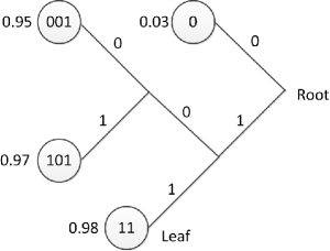
Figure 1: A tree source over ${\cal X}=\{0,1\}$. The states are ${\cal S}=\{0,11,001,101\}$ and the conditional probabilities are $p(x_{i}=1|0)=0.03$, $p(x_{i}=1|11)=0.98$, $p(x_{i}=1|001)=0.95$, and $p(x_{i}=1|101)=0.97$.

II-C Semi-predictive and two-pass source coding

Consider a tree source structure ${\cal S}$ whose explicit description requires $l_{{\cal S}}$ bits, and denote the probability of the input sequence $x$ conditioned on the tree source structure ${\cal S}$ by $p_{{\cal S}}(x)$. Using ${\cal S}$, the coding length required for $x$ is $l_{{\cal S}}-\log(p_{{\cal S}}(x))$. Define the MDL tree source structure ${\cal\widehat{S}}$ as the tree source structure that provides the shortest description of the data, i.e.,

$$\vspace*{-2mm}{\cal\widehat{S}}\triangleq\arg\min_{{\cal S}\in{\cal C}}\left\{l_{{\cal S}}-\log(p_{{\cal S}}(x))\right\},$$

where ${\cal C}$ is the class of tree source models being considered. The semi-predictive approach [12, 13, 14] processes the input $x$ in two phases. Phase I first estimates ${\cal\widehat{S}}$ by context tree pruning (CTP), which is a form of dynamic programming for coding length minimization (c.f. Baron [15] for details). The structure of $\widehat{{\cal S}}$ is then encoded explicitly. Phase II uses $\widehat{{\cal S}}$ to encode the sequence $x$ sequentially, where the parameters $\widehat{\Theta}$ are estimated while encoding $x$. The decoder first determines $\widehat{{\cal S}}$, and afterwards uses it to decode $x$ sequentially.

Two-pass MDL codes for tree sources describe both $\widehat{{\cal S}}$ and $\widehat{\Theta}$ in Phase I using CTP, and encode $x$ in Phase II. We use a two-pass approach instead of a semi-predictive approach, because estimating $B$ sets of parameters in parallel, one for encoding each of the $B$ blocks in Phase II, has $\rho(x)\approx 0.5B|{\cal S}|\log(N/B)$, whereas the two-pass approach has $\rho(x)\approx 0.5|S|\log(N)$, and the latter redundancy is smaller.

III Proposed Algorithm

We present a new Parallel Two-Pass MDL (PTP-MDL) algorithm. In order to keep the presentation simple, we restrict our attention to a binary alphabet, i.e., ${\cal X}=\{0,1\}$; the generalization to non-binary alphabets is straightforward. We will show that PTP-MDL has $O(N/B)$ time complexity when we restrict $D\leq\log(N/B)$, while still approaching the pointwise redundancy bound (1). This enables scalable data rates without a factor-$B$ increase in the redundancy.

III-A Overview

A block diagram of a possible implementation of the PTP-MDL encoder is shown in Fig. 2. In Phase I, the PTP-MDL encoder employs $B$ computational units called parallel units (PUs) that work in parallel to accumulate statistical information on $B$ blocks in $O(N/B)$ time, and a coordinating unit (CU) that controls the PUs and computes the MDL source estimate $\{\widehat{{\cal S}},\widehat{\Theta}\}$.

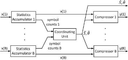
Figure 2: Block diagram of the PTP-MDL encoder.

Without loss of generality, we assume $N/B\in{\mathbb{Z}}^{+}$. Define the $B$ blocks as $x(1)=x_{1}^{N/B},x(2)=x_{N/B+1}^{2N/B},\ldots,x(B)=x_{N-N/B+1}^{N}$. PU $b$, where $b\in\{1,\ldots,B\}$, first computes for each depth-$D$ context $s$ the block symbol counts $n^{\alpha}_{s}(b)$, which are the number of times $\alpha$ is generated by $s$ in $x(b)$,

$$n^{\alpha}_{s}(b)\triangleq\sum_{i=(b-1)(N/B)+D+1}^{b(N/B)}1_{\left\{x_{i-D}^{i}=s\alpha\right\}},\alpha\in{\cal X},$$

where $s\alpha$ denotes concatenation of $s$ and $\alpha$. For each state $s$ such that $|s|<D$, the CU either retains the children states $0s$ and $1s$ in the MDL source, or prunes them and only retains $s$, whichever results in a shorter coding length. Details of the pruning decision appear in Section III-C3. Note that the serial MDL source considers the last $D$ symbols from the previous block as context for counting the first $D$ symbols of the current block (except the first block). However, using the serial MDL source is suboptimal in PTP-MDL, because this source does not reflect the actual symbols compressed by PTP-MDL.

In Phase II, each of the $B$ blocks is compressed by a PU. For each symbol $x_{i}(b)$, PU $b$ first determines the generator state $G_{i}(b)$, the state $s$ that generated the symbol $x_{i}(b)$. PU $b$ then assigns $x_{i}(b)$ a probability according to the parameters that were estimated by the CU in Phase I, and sequentially feeds the probability assignments to an arithmetic encoder [6].

The structure of the decoder is similar to that of Phase II. The approximated MDL source structure $\widehat{{\cal S}}$ and quantized parameters $\widehat{\Theta}$ are first derived from the parallel source description (see Section III-B). Then, the $B$ blocks are decompressed by $B$ decoding blocks. In decoding block $b$, each symbol $x_{i}(b)$ is sequentially decoded by determining $G_{i}(b)$, assigning a probability to $x_{i}(b)$ based on the parameter estimates, and applying an arithmetic decoder [6].

III-B Parallel source description

III-B1 Two-part codes in the PTP-MDL algorithm

Having received the block symbol counts $n^{\alpha}_{s}(b)$ from the PUs, the CU computes the symbol counts generated by state $s$ in the entire sequence $x$,

$$\vspace*{-2mm}n^{\alpha}_{s}=\sum_{b=1}^{B}n^{\alpha}_{s}(b),\qquad\alpha\in{\cal X}.$$ (2)

The CU can then compute the ML parameter estimates of $p(1|s)$ and $p(0|s)$,

$$\vspace*{-2mm}\theta_{s}\triangleq\theta_{s}^{1}=\frac{n_{s}^{1}}{n_{s}^{0}+n_{s}^{1}}\quad\quad\text{ and }\quad\quad\theta_{s}^{0}=1-\theta_{s}^{1},$$

respectively. The ML parameter estimates for each state $s$ are quantized into one of

$$K_{s}\triangleq\left\lceil\sqrt{2\pi^{2}\ln(2)\left(\frac{1}{2}-\frac{3}{16\ln(2)}\right)N}\right\rceil\approx\left\lceil 1.772\sqrt{N}\right\rceil$$ (3)

representation levels based on Jeffreys’ prior [16], where $\lceil\cdot\rceil$ denotes rounding up. The representation levels and bin edges are computed using a Lloyd-Max procedure [16]. The bin index and representation level for state $s$ are denoted by $k_{s}$ and $r_{s}$, respectively. Denoting the quantized ML estimate of $\theta_{s}^{\alpha}$ by $\widehat{\theta}_{s}^{\alpha}$, we have $\widehat{\theta}_{s}^{1}=r_{s}$ and $\widehat{\theta}_{s}^{0}=1-r_{s}$. Recall that, at the end of Phase I, the CU has computed the MDL structure estimate $\widehat{{\cal S}}$. If $s\in\widehat{{\cal S}}$, then the first part of the two-part code for symbols generated by $s$ consists of encoding $k_{s}$ with $\log(K_{s})$ bits. The WCR using this quantization approach is 1.047 bits per state above Rissanen’s redundancy bound [11, 16].

In Phase II, which implements the second part of the two-part code, each PU $b$ encodes its block $x(b)$ sequentially. For each symbol $x_{i}(b)$, PU $b$ determines $G_{i}(b)$. The symbol $x_{i}(b)$ is encoded according to the probability assignment $\widehat{p}(x_{i}(b))\triangleq\widehat{\theta}_{G_{i}(b)}^{x_{i}(b)}$ with an arithmetic encoder [6]. Thus, the probability assigned by all $B$ PUs to the symbols in $x$ whose generator state is $s$ is

$$\prod_{b=1}^{B}\prod_{\left\{i:\ G_{i}(b)=s,\ i>D\right\}}\widehat{p}(x_{i}(b))=(r_{s})^{n_{s}^{1}}(1-r_{s})^{n^{0}_{s}}.$$ (4)

Equation (4) provides the same redundancy for two-part codes in a parallel compression system as we would obtain in a serial system [15].

III-B2 Coding lengths in Phases I and II

In Phase I, the structure $\widehat{{\cal S}}$ is described with the natural code [5]. For a binary alphabet, $|\text{natural}_{\widehat{{\cal S}}}|\leq{2}|\widehat{{\cal S}}|-1$ bits; this is the model redundancy of PTP-MDL. The parameters $\widehat{\Theta}$ are described as the $|\widehat{{\cal S}}|$ indices $k_{s}$ in the order in which the leaves of $\widehat{{\cal S}}$ are reached in a depth-first search [9]; this description can be implemented with arithmetic coding [6]. The corresponding coding length is the parameter redundancy of PTP-MDL. We denote the length of the descriptions of $\widehat{{\cal S}}$ and $\widehat{\Theta}$ generated in Phase I by $l^{I}_{{\cal S}}$ bits. Using (3),

$$l^{I}_{{\cal S}} = |\text{natural}_{{\cal S}}|+|{\cal S}|\log(K_{s})$$

$$\lessapprox \left[2|{\cal S}|-1\right]+|{\cal S}|\left[\log(1.772)+\frac{1}{2}\log(N)\right].$$

In Phase II, the coding length is mainly determined by symbol probabilities conditioned on generator states as given by (4). There are two additional terms that affect the coding length in Phase II. First, coding redundancy for each arithmetic encoder with $\log(N)$ bits of precision requires $O(1)\leq 2$ bits [6]. Second, symbols with unknown context at the beginning of $x(b)$; we encode the first $D$ symbols of each block $x(b)$ directly using $D$ bits per block. Denoting the combined length of all $B$ codes in Phase II by $l^{II}_{{\cal S}}$ bits, we have

$$\vspace*{-2mm}l^{II}_{{\cal S}}\lessapprox B\cdot{(D+2)}-\sum_{s\in{\cal S}}[n_{s}^{1}\log(r_{s})+n_{s}^{0}\log(1-r_{s})].$$ (6)

Combining (III-B2) and (6), we have the following result for the redundancy.

Theorem 1

[15] The pointwise redundancy of the PTP-MDL algorithm over the ML entropy of the input sequence x w.r.t. the MDL souce structure $\widehat{S}$ satisfies

$$\rho(x)<B\left[\log\left(\frac{N}{B}\right)+2\right]+\frac{|\widehat{S}|}{2}\left[\log\left(N\right)+O\left(1\right)\right].$$

Note that the redundancy for naive parallel compression is upper bounded by $B\left[\log\left(\frac{N}{B}\right)+2+\frac{|\widehat{S_{n}}|}{2}\left[\log\left(N\right)+O\left(1\right)\right]\right]$, where $\widehat{S_{n}}$ is the estimated tree structure with the largest number of states among the $B$ tree structures.

III-C Phase I

III-C1 Computing block symbol counts

Computational unit $b$ computes $n^{\alpha}_{s}(b)$ for all $2^{D}$ depth-$D$ leaf contexts $s$. In order for PU $b$ to compute all block symbol counts in $O(N/B)$ time, we define the context index $c_{i}(b)$ of the symbol $x_{i}(b)$ as

$$c_{i}(b)\triangleq\sum_{j=0}^{D-1}2^{j}x_{j+i-D}(b),$$ (7)

where $i\in\{D+1,\ldots,N/B\}$ and $x_{j+i-D}(b)\in\{0,1\}$, hence $c_{i}(b)\in\{0,\ldots,2^{D}-1\}$. Note that $c_{i}(b)$ is the binary number represented by the context $s=x_{i-D}^{i-1}(b)$. Hence, it can be used as a pointer to the address containing the block symbol count $n_{s}^{\alpha}(b)$ for $s=x_{i-D}^{i-1}(b)$. Moreover, the property

$$c_{i+1}(b)=\frac{c_{i}(b)}{2}+2^{D-1}x_{i}(b)-\frac{x_{i-D}(b)}{2}$$ (8)

enables the computation of all $N/B-D$ context indices of the symbols of $x(b)$ in $O(N/B)$ time complexity.

III-C2 Constructing context trees

Because we restrict our attention to depth-$D$ contexts, it suffices for PU $b$ to compute $\{n^{\alpha}_{s}(b)\}_{\alpha\in{\cal X},\ s\in{\cal X}^{D}}$, all the block symbol counts of all the leaf contexts of a full depth-$D$ context tree. Information on internal nodes of the context tree, whose depth is less than $D$, is computed from the block symbol counts of the leaf contexts.

If $|s|=D$, then the CU gets $\{n^{\alpha}_{s}(b)\}_{\alpha\in{\cal X}}$ from the PUs and computes $n_{s}^{\alpha}$ with (2). Alternatively, $|s|<D$, the CU recursively derives $n_{s}^{\alpha}$ by adding up the symbol counts of children states, i.e.,

$$n_{s}^{\alpha}=n_{0s}^{\alpha}+n_{1s}^{\alpha},\qquad\forall\alpha\in{\cal X}.$$ (9)

III-C3 Computing the MDL source $\{\widehat{{\cal S}},\widehat{\Theta}\}$

For each state $s$, we either retain the children states $0s$ and $1s$ in the tree or merge them into a single state, according to which decision minimizes the coding length. The coding length $l_{s}$ of the two-part code that describes the symbols generated by $s$ is

$$l_{s}=\overbrace{\log(K_{s})}^{\text{Part~{}I}}\overbrace{-n^{0}_{s}\log(1-r_{s})-n^{1}_{s}\log(r_{s})}^{\text{Part~{}II}}.$$ (10)

We now derive the coding length required for state $s$, which is denoted by $\text{MDL}_{s}$. For $|s|=D$, $n_{s}^{0}$ and $n_{s}^{1}$ are computed with (2), $l_{s}$ is computed with (10), and $\text{MDL}_{s}=l_{s}$. For $|s|<D$, we compute $n_{s}^{\alpha}$ hierarchically with (9), after already having processed the children states. In order to decide whether to prune the tree, we compare $\text{MDL}_{0s}+\text{MDL}_{1s}$ with $l_{s}$. Because retaining an internal node requires the natural code [5] to describe that node (with $1$ bit),

$$\text{MDL}_{s}=\left\{\begin{matrix}l_{s}\quad\text{if $|s|=D$}\\ 1+\min\left\{\text{MDL}_{0s}+\text{MDL}_{1s},l_{s}\right\}&\text{else}\end{matrix}\right..$$

In terms of the natural code, if $|s|=D$, then $s$ is a leaf of the full depth-$D$ context tree, and its natural code is empty; else $|s|<D$, and the natural code requires $1$ bit to encode whether $s\in{\cal S}$. The symbols generated by $s$ are encoded either by retaining the children states (this requires a coding length of $\text{MDL}_{0s}+\text{MDL}_{1s}$ bits), or by pruning the children states and retaining state $s$ with coding length $l_{s}$. If $|s|=D$, then we do not process deeper contexts. The CTP has $O(N/B)$ time complexity because the tree has $O(N/B)$ states.

III-D Phase II

In Phase II, PU $b$ knows $\widehat{{\cal S}}$ and $\{r_{s}\}_{s\in\widehat{{\cal S}}}$. PU $b$ encodes $x(b)$ sequentially; for each symbol $x_{i}(b)$, it determines $G_{i}(b)$. An $O(N/B)$ algorithm for determining $G_{i}(b)$ for all the symbols of $x(b)$ utilizing (7,8) is described by Baron [15]. After determining $G_{i}(b)$, the symbol $x_{i}(b)$ is encoded according to the probability assignment $\widehat{p}(x_{i}(b))\triangleq\widehat{\theta}_{G_{i}(b)}^{x_{i}(b)}$ with an arithmetic encoder [6]. In order to have $O(N/B)$ time complexity and $O(1)$ expected coding redundancy per PU, arithmetic coding is performed with $\log(N)$ bits of precision [6], where we assume that the hardware architecture performs arithmetic with $\log(N)$ bits of precision in $O(1)$ time.

III-E Decoder

The $B$ decoding blocks can be implemented on $B$ PUs. Decoding block $b$ decodes $x(b)$ sequentially; for each symbol $x_{i}(b)$, it determines $G_{i}(b)$. The same $O(N/B)$ algorithm used in Phase II for determining $G_{i}(b)$ for all the symbols of $x(b)$ can be used in the $B$ decoding blocks. After determining $G_{i}(b)$, the symbol $x_{i}(b)$ is decoded according to the probability assignment $\widehat{p}(x_{i}(b))\triangleq\widehat{\theta}_{G_{i}(b)}^{x_{i}(b)}$ with an arithmetic decoder [6] that has $O(N/B)$ time complexity.

Theorem 2

[15] With computations performed with $\log(N)$ bits of precision defined as $O(1)$ time, the PTP-MDL encoder and decoder each require $O(N/B)$ time.

IV Numerical Results

This last section presents numerical results that compare the coding lengths of the parallel two-pass and naive parallel algorithms for different encoder settings and different numbers of parallel blocks. Two encoders are considered: MDL encoder (context tree pruning), and full depth Markov encoder (no pruning).

We test the average coding lengths over 2,000 repetitions for signals of length $N=10,000$ generated by the context tree source with $4$ states as described in Fig. 1. The maximum context depth $D$ is set to be $5\leq\log\left(N/B\right)$ for both MDL and Markov encoders. Hence the Markov encoder will run with $2^{5}=32$ states. For the MDL encoder, context tree pruning estimates the number of states $|\widehat{S}|$ to be around $4$, which is the number of states in the original source. Note that the coding length for a Bernoulli encoder, which uses $D=0$, is greater than the coding lengths of the other encoders, and hence is not included in our results.

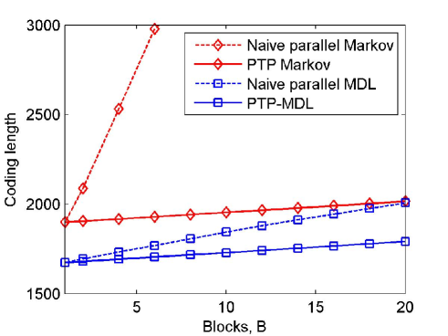
Figure 3: The performance of PTP and naive parallel compression algorithms using MDL and Markov encoders.

Fig. 3 shows our numerical results. It can be seen that PTP-MDL gives the best compression among the encoders, because the redundancy due to the source description $l^{I}_{{\cal S}}$ is higher for the Markov source than the MDL source due to the larger number of states.

Comparing the coding lengths for PTP-MDL and naive parallel compression, we can see that the rate of increase in coding length is higher for naive parallel compression. Both PTP-MDL and naive parallel compression suffer from the same coding redundancy, and redundancy due to unknown context for each block. However, the parameter redundancy due to source description is approximately $B$ times larger for naive parallel than for PTP-MDL.

In summary, for context tree sources of depth $D\leq\log\left(N/B\right)$, PTP-MDL can compress data in $O(N/B)$ time while achieving a redundancy within $B\log(N/B)$ bits above Rissannen’s lower bound on universal coding performance.

References

- [1] S. Arming, R. Fenkhuber, and T. Handl, “Data compression in hardware – the Burrows-Wheeler approach,” in IEEE Int. Symp. Des. Diagnostics Electron. Circuits Syst., Apr. 2010, pp. 60–65.
- [2] P. Franaszek, J. Robinson, and J. Thomas, “Parallel compression with cooperative dictionary construction,” in Proc. Data Compression Conf. (DCC), Mar. 1996.
- [3] A. Beirami and F. Fekri, “On lossless universal compression of distributed identical sources,” in Proc. Int. Symp. Inf. Theory (ISIT), July 2012, pp. 561–565.
- [4] M. L. A. Stassen and T. J. Tjalkens, “A parallel implementation of the CTW compression algorithm,” in Proc. 22d Benelux Symp. Inf. Comm., May 2001, pp. 85–92.
- [5] F. M. J. Willems, Y. M. Shtarkov, and T. J. Tjalkens, “The context tree weighting method: Basic properties,” IEEE Trans. Inf. Theory, vol. 41, no. 3, pp. 653–664, May 1995.
- [6] T. M. Cover and J. A. Thomas, Elements of Information Theory, New York, NY, USA: Wiley-Interscience, 2006.
- [7] F. M. J. Willems, “Some challenges in source coding,” in Proc. 3rd ITG Conf. Source Channel Coding, Jan. 2000, pp. 245–249.
- [8] J. Rissanen, “Modeling by shortest data description,” Automatica, vol. 14, no. 5, pp. 465–471, Sept. 1978.
- [9] T. H. Cormen, C. E. Leiserson, and R. L. Rivest, Introduction to Algorithms, The MIT Press, Cambridge, MA, 2009.
- [10] M. J. Weinberger, N. Merhav, and M. Feder, “Optimal sequential probability assignment for individual sequences,” IEEE Trans. Inf. Theory, vol. 40, no. 2, pp. 384–396, Mar. 1994.
- [11] J. Rissanen, “Fisher information and stochastic complexity,” IEEE Trans. Inf. Theory, vol. 42, no. 1, pp. 40–47, Jan. 1996.
- [12] D. Baron and Y. Bresler, “An O(N) semipredictive universal encoder via the BWT,” IEEE Trans. Inf. Theory, vol. 50, no. 5, pp. 928–937, May 2004.
- [13] P. A. J. Volf and F. M. J. Willems, “A study of the context tree maximizing method,” in Proc. 16th Benelux Symp. Inf. Theory, Nieuwerkerk Ijsel, Netherlands, 1995, pp. 3–9.
- [14] F. M. J. Willems, Y. M. Shtarkov, and T. J. Tjalkens, “Context-tree maximizing,” in Proc. Conf. Inf. Sci. Syst., Mar. 2000, pp. 7–12.
- [15] D. Baron, “Fast parallel algorithms for universal lossless source coding,” Feb. 2003, Ph.D. thesis, UIUC.
- [16] D. Baron, Y. Bresler., and M. K. Mihcak, “Two-part codes with low worst-case redundancies for distributed compression of Bernoulli sequences,” in Proc. Conf. Inf. Sciences Systems, Mar. 2003.