Fundamental properties of solar-like oscillating stars from frequencies of minimum $\Delta\nu$: I. Model computations for solar composition

Abstract

Low amplitude is the defining characteristic of solar-like oscillations. The space projects $Kepler$ and $CoRoT$ give us a great opportunity to successfully detect such oscillations in numerous targets. Achievements of asteroseismology depend on new discoveries of connections between the oscillation frequencies and stellar properties. In the previous studies, the frequency of the maximum amplitude and the large separation between frequencies were used for this purpose. In the present study, we confirm that the large separation between the frequencies has two minima at two different frequency values. These are the signatures of the He II ionization zone, and as such have very strong diagnostic potential. We relate these minima to fundamental stellar properties such as mass, radius, luminosity, age and mass of convective zone. For mass, the relation is simply based on the ratio of the frequency of minimum $\Delta\nu$ to the frequency of maximum amplitude. These frequency comparisons can be very precisely computed, and thus the mass and radius of a solar-like oscillating star can be determined to high precision. We also develop a new asteroseismic diagram which predicts structural and evolutionary properties of stars with such data. We derive expressions for mass, radius, effective temperature, luminosity and age in terms of purely asteroseismic quantities. For solar-like oscillating stars, we now will have five very important asteroseismic tools ( two frequencies of minimum $\Delta\nu$, the frequency of maximum amplitude, and the large and small separations between the oscillation frequencies) to decipher properties of stellar interior astrophysics.

1 Introduction

Every object in the universe oscillates in its own way. For stars, the increasing sensitivity in detecting oscillations in solar-like objects by the space missions $Kepler$ and $CoRoT$ is ushering in a new era in stellar astrophysics. Determination of fundamental properties of single stars from oscillation frequencies ($\nu$) is among the promises of asteroseismology. The relation between the mean density and the large separation between the oscillation frequencies (${\Delta\nu}$) is well known (Ulrich 1986). Kjeldsen & Bedding (1995) proposed a semi-empirical relation between fundamental properties of stars and the frequency of maximum amplitude ($\nu_{\rm max}$). In the present study, we suggest two new frequencies ($\nu_{\rm min1}$ and $\nu_{\rm min2}$) which, together with $\nu_{\rm max}$ and the mean of ${\Delta\nu}$ ($\left<\Delta\nu\right>$), can be used to derive expressions for these fundamental properties. $\nu_{\rm min1}$ and $\nu_{\rm min2}$ are the frequencies at which $\Delta\nu$ is minimum. We will show that they have excellent predictive power for stellar mass ($M$), radius ($R$) and effective temperature ($T_{\rm eff}$) of single stars, especially if the observations yield accurate values of $\nu_{\rm max}$.

Kjeldsen & Bedding (1995) estimate amplitudes of solar-like oscillations and then interrelate $\nu_{\rm max}$ and $\left<\Delta\nu\right>$ to the stellar mass and radius. Relatively simple expressions for $M$ and $R$ as can be written as functions of $\nu_{\rm max}$, $\left<\Delta\nu\right>$ and $T_{\rm eff}$ (e.g. see Chaplin et al. 2011):

$$\frac{M}{{\rm M}_{\sun}}=\frac{(\mbox{$\nu_{\rm max}$}/\mbox{$\nu_{\rm max\sun}$})^{3}}{(\left<\mbox{$\Delta\nu$}\right>/\left<\Delta\nu_{\sun}\right>)^{4}}\left(\frac{T_{\rm eff}}{\rm T_{eff\sun}}\right)^{1.5},$$ (1)

$$\frac{R}{{\rm R}_{\sun}}=\frac{(\mbox{$\nu_{\rm max}$}/\mbox{$\nu_{\rm max\sun}$})}{(\left<\mbox{$\Delta\nu$}\right>/\left<\Delta\nu_{\sun}\right>)^{2}}\left(\frac{T_{\rm eff}}{\rm T_{eff\sun}}\right)^{0.5}.$$ (2)

These expressions for $M$ and $R$ are applied in many studies. $Kepler$ and $CoRoT$ data provide us $\Delta\nu$  and $\nu_{\rm max}$ for enough stars to confirm that there is a significant difference between the mass found from modelling of these stars and their mass given by equation (1) (see, e.g., Mathur et al. 2012). Although a number of papers are dedicated to new scaling relations to remove this difference (Chaplin et al. 2011; Huber et al. 2011b; Kjeldsen & Bedding 2011; Stello et al. 2011; Corsaro et al. 2013), it is still uncertain if these relations are sufficient as written, or are sensitive to other stellar parameters not included in them (see, e.g., White et al. 2011). The scaling relation may depend on, for example, metallicity (see section 5.8).

For some of the hottest F-type stars, it is reported that power envelopes have a flatter maximum (see, e.g., Arentoft et al. 2008; Chaplin & Miglio 2013). For Procyon, for example, photometric and spectroscopic methods give different $\nu_{\rm max}$ values: $\nu_{\rm max,phot}=1014~{}{\mbox{${\rm\mu}$Hz}}$, $\nu_{\rm max,RV}=923~{}\mbox{${\rm\mu}$Hz}$ (Huber et al. 2011a). For such extreme stars, it is difficult to use the scaling relations given in equations (1) and (2). For the stars later than F-type, however, $\nu_{\rm max}$ is much more precisely determined from the observations than for the hot F-type stars.

Sound speed throughout a star changes due to a variety of factors. Abrupt variations can occur due to structural reasons, e.g., transformation between the energy transportation mechanisms and ionic states of certain elements. It is thought that such acoustic glitches induce an oscillatory component in the spacing of oscillation frequencies (Houdek & Gough 2011; Mazumdar et al. 2012). In particular, changes in physical conditions in the He II ionization zone are very efficient in creating detectable glitches. Variations of $\Delta\nu$  around the minima are almost entirely shaped by variations of the first adiabatic exponent throughout the zone (see Section 4).

In this paper we suggest two new frequencies and show their diagnostic potential by relating them with the fundamental stellar parameters. The paper is organized as follows. In Section 2 the basic properties of stellar interior models and Ankara-İzmir (ANKİ) stellar evolution code used in construction of these models are presented. Section 3 is devoted to analysis of oscillation frequencies, the method for determination of $\nu_{\rm min}$₁ and $\nu_{\rm min}$₂, and diagnostic potentials of the reference frequencies and their mode order differences. In Section 4, we consider how the He II ionization zone influences oscillation frequencies and hence their spacing. Section 5 deals with relating the asteroseismic quantities to the fundamental properties of stars. Finally, in Section 6, we draw our conclusions.

2 Properties of the ANKİ code and Models

2.1 Properties of the ANKİ code

The models used in the present asteroseismic analysis are constructed by using the ANKİ code (Ezer & Cameron 1965). Convection is treated with standard mixing-length theory (Böhm-Vitense 1958) without overshooting. ANKİ solves the Saha equation for hydrogen and helium, and computes the equation of state by using the Mihalas et al. (1990) approach for survival probabilities of energy levels (Yıldız & Kızıloğlu 1997). The radiative opacity is derived from recent OPAL tables (Iglesias & Rogers 1996), supplemented by the low-temperature tables of Ferguson et al. (2005). Nuclear reaction rates are taken from Angulo et al. (1999) and Caughlan & Fowler (1988). Although rotating models (Yıldız 2003, 2005) and models with microscopic diffusion (Yıldız 2011; Metcalfe et al. 2012) can be constructed by using ANKİ, these effects are not included in the model computations for this study. For only the solar model, diffusion is taken into account in order to use its known values for the convective parameter ($\alpha$), hydrogen ($X$) and heavy element ($Z$) abundances.

2.2 Properties of Models

Interior models are constructed by using the ANKİ code. The mass range of models is 0.8-1.3 M_☉ with mass step of 0.05 M_☉. The chemical composition is taken as the solar composition: $X=0.7024$ and $Z=0.0172$. The heavy element mixture is assumed to be the solar mixture given by Asplund et al. (2009). The solar value of the convective parameter $\alpha$ for ANKİ  is used: $\alpha=1.98$.

We have computed adiabatic oscillation frequencies by using ADIPLS oscillation package (Christensen-Dalsgaard, 2008) for each mass when the central hydrogen is reduced to $X_{\rm c}=0.7$, $0.53$, $0.35$ and $0.17$. We can compare models with different masses having the same relative age ($t_{\rm rel}$). Define $t_{\rm MS}$ as the main-sequence (MS) lifetime of a star. Then, for a star having age $t$, relative age becomes $t_{\rm rel}=t/t_{\rm MS}$. The first value of $X_{\rm c}$ marks essentially the zero-age main sequence (ZAMS) age of each stellar mass and therefore $t_{\rm rel}$ is very small. By definition, $t_{\rm rel}=1$ for terminal-age main sequence (TAMS) models. The other $X_{\rm c}$ values ($0.53$, $0.35$, $0.17$), however, nearly correspond to $t_{\rm rel}\approx 0.3$, $0.5$ and $0.75$, respectively.

In the construction of solar models, diffusion is taken into account. The maximum sound speed difference between the solar model and the Sun is 1.7 per cent. The base radius of convective zone (CZ) and surface helium abundance are 0.732 R_☉ and 0.25, respectively. These values are moderately in agreement with the inferred values from solar oscillations: 0.713 R_☉ and $Y_{\rm s}=0.25$ (Basu & Antia, 1995; Basu & Antia, 1997). Improved solar models (and also models for $\alpha$ Cen A and B) by using ANKİ are obtained by opacity enhancement (Yıldız 2011).

3 Frequencies of minimum $\Delta\nu$ and their diagnostic potential

Figure 1: Variation of $\Delta\nu$ as a function of $\nu$ for the BiSON solar data (Chaplin et al. 1999) for $l=0$, $1$ and $2$.

Figure 2: $\Delta\nu$ as a function of $\nu$ for solar model for $l=0$, $1$ and $2$.

Figure 3: $\Delta\nu$ as a function of $\nu$ for 1.0-1.3 ${\rm M}_{\sun}$ models with $X_{\rm c}=0.35$. The degree of the modes is $l=0$ for all of the models.

The asymptotic relation describes the relation between frequency of a mode ($\nu_{nl}$) and its order ($n$) and degree ($l$). According to this relation, the large separation between the frequencies ($\Delta\nu=\nu_{nl}-\nu_{n-1,l}$) is to a great extent constant. This is true for the Sun and other solar-like oscillating stars. We compute $\left<\Delta\nu\right>$ in the mode order range $n=10-25$. $\Delta\nu$ is plotted with respect to $n$ and a constant function is fitted. For the BiSON solar data (Chaplin et al. 1999), $\left<\Delta\nu\right>_{\sun}=135.11$ ${\rm\mu}$Hz for $l=0$ and $\left<\Delta\nu\right>_{\sun}=135.17$ ${\rm\mu}$Hz for $l=1$. These results show that $\left<\Delta\nu\right>$ is independent of $l$. In this study we compute $\left<\Delta\nu\right>$ from the modes with $l=0$. The range of $\Delta\nu$ for degree $l=0$ is 133-138 ${\rm\mu}$Hz. Although this is a very small interval, there are very significant changes through it. Variation of $\Delta\nu$ with the frequency is plotted in Fig. 1 for $l=0$, 1 and 2. The aim of this paper is to make links between such changes and stellar parameters. The common feature of the three curves is that there are two minima. We call the minimum having high frequency as the first minimum and the other one as the second minimum. The frequency of the first minimum ($\nu_{\rm min1}$) is around 2600 ${\rm\mu}$Hz, and the second ($\nu_{\rm min2}$) is around 1900 ${\rm\mu}$Hz. Do these minima also exist in the eigenfrequencies of a solar model? In Fig. 2, $\Delta\nu$ of 1.0 M_☉ model is plotted with respect to $\nu$ for three values of $l$ when $X_{\rm c}=0.35$. We confirm that both of the minima seen in the Sun also exist for the oscillation frequencies of 1 M_☉ model. We now consider whether this kind of variation also appears in $\Delta\nu-\nu$ graphs for other solar-like oscillating stars of different mass.

In Fig. 3, $\Delta\nu$ is plotted with respect to $\nu$ for 1.0, 1.1, 1.2 and 1.3 M_☉ interior models with $X_{\rm c}=0.35$. The eigenfrequencies are for the $l=0$ modes. This is the case throughout this paper, if not otherwise stated. The values of $\nu_{\rm min}$₁ and $\nu_{\rm min}$₂ for 1.0 and 1.3 M_☉  models are marked in the figure. As mass increases the minima regularly shift towards lower frequencies. While $\nu_{\rm min}$₁ is 2600 ${\rm\mu}$Hz for the Sun, $\nu_{\rm min}$₁ for a 1.3 M_☉ model is about 2000 ${\rm\mu}$Hz. $\nu_{\rm min}$₂ for the Sun is about 1900 ${\rm\mu}$Hz and it is about 1500 ${\rm\mu}$Hz  for the 1.3M_☉ model. The ZAMS model of a 1 M_☉ model has $\nu_{\rm min}$₁= 3400 ${\rm\mu}$Hz  and $\nu_{\rm min}$₂= 2500 ${\rm\mu}$Hz. For interior models of stellar mass up to 1.4 M_☉, the minima shift again towards lower frequencies as model evolves within the MS.

3.1 Determination of $\nu_{\rm min}$₁ and $\nu_{\rm min}$₂

For oscillating stars, we have a discrete set of eigenfrequencies. In such a case, say, $\nu_{\rm min}$₁ does not have to correspond with any of the eigenfrequencies. Then we must determine where the minimum occurs in the $\Delta\nu-\nu$ graph. Suppose $\nu_{\rm min}$₁ is in between the frequencies $\nu_{1}$ and $\nu_{2}$. We use the slopes of the frequency intervals adjacent to $\nu_{1}$ and $\nu_{2}$ to determine $\nu_{\rm min}$₁. The intersection point of these two lines gives us value of $\nu_{\rm min}$₁. In Fig. 4 two examples for the determination of $\nu_{\rm min}$₁ are sketched. These are 1.0 M_☉ models with $X_{\rm c}=0.17$ and $0.35$.

Figure 4: Method for determination of the minima’s frequencies. The two examples are 1.0 M_☉ models with $X_{\rm c}=0.17$ and $0.35$. We first determine frequency interval of the minimum and draw two lines from the neighbourhood intervals. The intersection of these two lines gives us $\nu_{\rm min}$₁.

Figure 5: $\epsilon_{3}$ (equation 3) as a function of $\nu$ for the Sun and solar model for $l=0$.

In Figs 1 and 2, it is shown that there are three very similar curves for $\Delta\nu$ for different values of oscillation degree $l$ ($l=0$, $1$ and $2$). However, the values of $\nu_{\rm min1}$ for different $l$ are slightly different. Such a difference may be considered as negligibly small but it may be important if one wants to determine fundamental stellar parameters. Therefore, we should try to find a single value for $\nu_{\rm min1}$. In Fig. 5, the frequency difference parameter $\epsilon_{3}$ is plotted with respect to $\nu$. Here, $\epsilon_{3}$ is defined as

$$\epsilon_{3}=\prod_{l=0}^{2}(\Delta\nu_{l}-{\left<\Delta\nu\right>})$$ (3)

where $\Delta\nu_{l}$ is the large separation for degree $l$. For each $n$, $(\Delta\nu_{0}-{\left<\Delta\nu\right>})(\Delta\nu_{1}-{\left<\Delta\nu\right>})(\Delta\nu_{2}-{\left<\Delta\nu\right>})$ is computed. $\epsilon_{3}$ has a much clearer minimum than $\Delta\nu$. This minimum is the first minimum. The second minimum for the Sun is missing in Fig. 5 because it is very shallow. The frequency of the first minimum for the Sun from $\epsilon_{3}$ is obtained as 2493.2 ${\rm\mu}$Hz for the BiSON data. However, in some evolved stars, the mixed modes that are observed render this method inapplicable.

3.2 The diagnostic potential of the mode order difference

Figure 6: The mass of the CZ and $T_{\rm eff}$ as a function of the mode order difference between $\nu_{\rm max}$  and $\nu_{\rm min}$₁, $\Delta n_{\rm x1}=(\mbox{$\nu_{\rm max}$}-\mbox{$\nu_{\rm min}$}_{1})/\mbox{$\Delta\nu$}$. The negative values of $\Delta n_{\rm x1}$ correspond models with $M>1.2{\rm M}_{\sun}$. $M_{\rm CZ}$ of these models is very low. The thin solid line represents the fitted line for the range of $\Delta n_{\rm x1}=0$$-9$, $M_{\rm CZ}/{\rm M}_{\sun}=0.066\Delta n_{\rm x1}$. The thick solid line shows the fitted line for $T_{\rm eff}$ found as $T_{{\rm eff},\Delta n}=(1.142-9.63~{}10^{-3}(\Delta n_{\rm x1}+4)^{1.35}){\rm T_{eff\sun}}$.

The relation between the frequencies of two minima is approximately given as

$${\nu_{\rm min1}}\simeq 1.36\nu_{\rm min2}.$$ (4)

Although the order of oscillation modes is not determined from observations, the existence of $\nu_{\rm min}$ may solve this problem, entirely or in part. Both $\nu_{\rm min1}$ and $\nu_{\rm min2}$ shift regularly as stellar mass and age change. The difference between $\nu_{\rm min1}$ and $\nu_{\rm min2}$ of the models we consider is

$$\Delta n_{12}=n_{1}-n_{2}=(\nu_{\rm min1}-\nu_{\rm min2})/\left<\Delta\nu\right>=5-6.$$ (5)

Its mean value is 5.6. The value of $\Delta n_{12}$ is a function of both $M$ and $t$. However, the depth of the CZ, $d_{\rm BCZ}=(R_{\star}-R_{\rm BCZ})/R_{\star}$, is also a function of $M$ and $t$. Here, $R_{\star}$ and $R_{\rm BCZ}$ are the stellar radius and base radius of the convective zone (BCZ). Indeed, there is a linear relation between $\Delta n_{12}$ and $1/d_{\rm BCZ}$. $\Delta n_{12}$ is about 5 when $d_{\rm BCZ}\approx 0.3$ and $\Delta n_{12}$ is about 7 when $d_{\rm BCZ}\approx 0.1$.

For the mass of the CZ, however, a stringent relation is found with the mode order difference ($\Delta n_{\rm x1}$) between $\nu_{\rm max}$  and $\nu_{\rm min}$₁. We define $\Delta n_{\rm x1}$ as

$$\Delta n_{\rm x1}=(\nu_{\rm max}-\nu_{\rm min1})/\left<\Delta\nu\right>.$$ (6)

Mass of CZ ($M_{\rm CZ}$) is plotted with respect to $\Delta n_{\rm x1}$ in Fig. 6. For the models of mass $M<1.2{\rm M}_{\sun}$, there is a linear relation between $M_{\rm CZ}$ and $\Delta n_{\rm x1}$, at least for the MS stars. This relation arises from the fact that both $M_{\rm CZ}$ and $\Delta n_{\rm x1}$ are related to $T_{\rm eff}$. It is a very strict constraint for interior models of solar-like oscillating stars. While $M_{\rm CZ}$ of the 1.0 M_☉   model with X${}_{\rm c}=0.35$ is 0.025 M_☉, the fitting curve gives it as 0.024 M_☉. For the MS models of mass $M>1.2{\rm M}_{\sun}$ ($\Delta n_{\rm x1}<0$ ), $M_{\rm CZ}$ is negligibly small and therefore the method is not applicable.

A similar method can also be obtained for $\Delta n_{\rm x2}=(\nu_{\rm max}-\nu_{\rm min2})/\left<\Delta\nu\right>$, the difference between $\nu_{\rm max}$ and $\nu_{\rm min2}$. The fitting curve for $M_{\rm CZ}$ is $M_{\rm CZ}=0.0091\Delta n_{\rm x2}-0.0540$. For the model given above $M_{\rm CZ}$ is found from $\Delta n_{\rm x2}$ as 0.025. This result is in good agreement with $M_{\rm CZ}$ obtained from $\Delta n_{\rm x1}$. One can take the mean value of $M_{\rm CZ}$ from $\Delta n_{\rm x1}$ and $\Delta n_{\rm x2}$ as a constraint to interior models of solar-like oscillating stars.

In Fig.6, $T_{\rm eff}$ is also plotted with respect to $\Delta n_{\rm x1}$. There is an inverse relation between $T_{\rm eff}$ and $\Delta n_{\rm x1}$: $T_{{\rm eff},\Delta n}=(1.142$$-9.63~{}10^{-3}(\Delta n_{\rm x1}+4)^{1.35}){\rm T_{eff\sun}}$. This relation is very definite and may be used to infer $T_{\rm eff}$ from asteroseismic quantities alone. The difference between $T_{{\rm eff},\Delta n}$ and model $T_{\rm eff}$ is less than 100 K.

4 Signature of the HeII ionization zone on the asymptotic relation

The sound speed within a stellar interior is given as $c=\sqrt{\Gamma_{1}\frac{P}{\rho}}$. The first adiabatic exponent $\Gamma_{1}$ is to a great extent constant and very close to $5/3$ in the deep solar interior. Near the surface, however, an abrupt change in $\Gamma_{1}$ occurs at about $0.98$ R_☉, as a signature of the He II ionization zone. Such a change significantly influences the sound speed profile near the stellar surface and behaves as an acoustical glitch for the oscillation frequencies.

The effect of the acoustical glitch induced by the second helium ionization zone on the oscillation frequencies is extensively discussed in the literature (see e.g., Perez Hernandez & Christensen-Dalsgaard 1994, 1998). In particular, Dziembowski, Pamyatnykh & Sienkiewicz (1991), Vorontsov, Baturin & Pamyatnykh (1991), Perez Hernandez & Christensen-Dalsgaard (1994) successfully obtained the helium abundance in the solar envelope from the phase function for solar acoustic oscillations (see also Monteiro & Thompson 2005). Houdek & Gough (2007) consider the second difference as a diagnostic of the properties of the near-surface region. In this section we consider how the glitch shapes the variation of $\Delta\nu$  with respect to $\nu$.

The large frequency separation of a star depends on the sound speed profile in its interior. It can be written down in terms of acoustic radius as

$$\mbox{$\Delta\nu$}=\left(2\int_{0}^{R}\frac{{\rm d}r}{c}\right)^{-1},$$ (7)

where acoustic radius $\int\frac{{\rm d}r}{c}$ is the required time for sound waves to travel from the centre to the surface.

As stated above the acoustic glitches induce an oscillatory component in the spacing of oscillation frequencies. Therefore, we are facing a deviation from the asymptotic relation. The reason of the oscillatory component is essentially due to coincidence of the He II ionization with the peaks between the radial nodes.

Let $\xi_{\rm r}$ be the radial component of the displacement vector. It gives us the positions of the radial nodes. The solution of the second order differential equation yields (Christensen-Dalsgaard 2003)

$$\xi_{\rm r}=\frac{A}{r(\rho c)^{1/2}}\left|\frac{S_{l}^{2}/\omega^{2}-1}{N^{2}/\omega^{2}-1}\right|^{1/4}\cos\left(\int_{r}^{r_{2}}K(r)^{1/2}{\rm d}r-\frac{\rm\pi}{4}\right),$$ (8)

where $r_{2}$ is the outer turning point and

$$K(r)=\frac{\omega^{2}}{c^{2}}\left(\frac{N^{2}}{\omega^{2}}-1\right)\left(\frac{S_{l}^{2}}{\omega^{2}}-1\right).$$ (9)

In this equation, $\omega$ is the eigenfrequency obtained from solution of the wave equation. $c$, $N$ and $S_{l}$ are sound speed, Brunt-Väisälä and the characteristic acoustic frequencies, respectively.

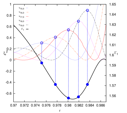
Figure 7: Square of the radial component (equation 8) of the displacement vector is plotted against the relative radius for the eigenfrequencies of 1.0 M_☉ model with $X_{\rm c}=0.35$ around its $\nu_{\rm min}$₁. The amplitude $A$ in equation (8) is arbitrarily chosen to obtain $\xi_{\rm r}^{2}$ about unity. Also plotted is the first adiabatic exponent $\Gamma_{1}$ (thick solid line). $\Gamma_{1}$ has a local minimum about $r=0.98$, due to the He II ionization zone. The location of the local peak in $\xi_{\rm r}^{2}$ relative to the dip in $\Gamma_{1}$ determines the departure of the frequencies from the asymptotic relation, with a decrease in the frequency that is larger, the closer the peak is to the minimum in $\Gamma_{1}$. While the circles show peaks of the oscillations, the filled circles represent their projections on $\Gamma_{1}$.

The influence of the He II ionization zone on $\Delta\nu$  can be understood from Fig. 7. Square of $\xi_{\rm r}$, given in equation (8), is plotted with respect to relative radius around the zone, for eigenfrequencies of the 1.0 M_☉ model with $X_{\rm c}=0.35$ near $\nu_{\rm min}$₁. Also seen is the first adiabatic exponent $\Gamma_{1}$. The horizontal axis is chosen so that the effect of the zone on $\Gamma_{1}$ is clearly shown. In the zone, $\Gamma_{1}$ has a local minimum where number of He II is the same as number of He III. The largest deviation from the asymptotic relation occurs for the mode that has one of its peaks closest to the minimum. This is the mode with $n=17$. $\nu_{\rm min}$₁ is between $\nu_{17,0}$ and $\nu_{18,0}$ (see also Fig. 4). We note that the minimum of $\Gamma_{1}$ takes place between the points where $\xi_{\rm r}^{2}$ of modes with $n=17$ and $18$ is maximum. Therefore, variation of $\Gamma_{1}$ in the He II ionization zone shapes the variation of $\Delta\nu$. In order to relate quantitatively the expected local frequency decrease for specific modes to the minima in $\Delta\nu$, further analysis is required.

5 Stellar parameters from asteroseismic frequencies

5.1 The relations between the reference frequencies

Figure 8: $\nu_{\rm min1}/\nu_{\rm min1\sun}$ with respect to $\nu_{\rm max}/\nu_{\rm max\sun}$. The circles show the models with $X_{\rm c}=0.7$, while the filled circles are for the models with lower values of $X_{\rm c}$. The numbers represent the model masses in solar units.

Figure 9: $\nu_{\rm min1}{\rm M}_{\sun}/\nu_{\rm min1\sun}M$ (filled circle) and $\nu_{\rm min2}{\rm M}_{\sun}/\nu_{\rm min2\sun}M$ (circle) are plotted with respect to $\nu_{\rm max}/\nu_{\rm max\sun}$. This shows that $\nu_{\rm min1}{\rm M}_{\sun}/\nu_{\rm min1\sun}M=\nu_{\rm max}/\nu_{\rm max\sun}$. This equality is a very important tool for computation of stellar mass using asteroseismic methods.

In our analysis, $\nu_{\rm max}$ of models is computed from equation (1), using model values of $\left<\Delta\nu\right>$, $T_{\rm eff}$ and $M$. In Fig. 8, $\nu_{\rm min1}/\nu_{\rm min1\sun}$ is plotted with respect to $\nu_{\rm max}/\nu_{\rm max\sun}$. The solar values of $\nu_{\rm min1\sun}$ and $\left<\mbox{$\Delta\nu$}_{\sun}\right>$ are found from the BiSON data as 2555.18 and 135.11 ${\rm\mu}$Hz, respectively. $\nu_{\rm max\sun}$ is taken as 3050 ${\rm\mu}$Hz. The dotted line is for $\nu_{\rm min1}/\nu_{\rm min1\sun}=\nu_{\rm max}/\nu_{\rm max\sun}$. They are correlated but there is no one-to-one relation. However, we confirm that the difference between $\nu_{\rm min1}/\nu_{\rm min1\sun}$ and $\nu_{\rm max}/\nu_{\rm max\sun}$ increases as stellar mass is different from 1.0 M_☉. The closest models to the dotted line are 1.0 M_☉ models. If we plot $\nu_{\rm min1}{\rm M}_{\sun}/\nu_{\rm min1\sun}M$ with respect to $\nu_{\rm max}/\nu_{\rm max\sun}$, a linear relation is obtained. In Fig. 9, $\nu_{\rm min1}{\rm M}_{\sun}/\nu_{\rm min1\sun}M$ (filled circle) is plotted with respect to $\nu_{\rm max}/\nu_{\rm max\sun}$. It is shown that $\nu_{\rm min2}$ obeys the same relation with $\nu_{\rm max}$ as $\nu_{\rm min1}$. The solar value of $\nu_{\rm min2\sun}$ is taken as 1879.52 ${\rm\mu}$Hz, again from the BiSON data. This implies that $\nu_{\rm min1}/M$ and $\nu_{\rm min2}/M$ are equivalent to each other. Furthermore, they can be used with and without $\nu_{\rm max}$ in new scaling relations.

5.2 Stellar mass from just ratio of the frequency of minimum $\Delta\nu$ to the frequency of maximum amplitude

A very important result one can deduce from Fig. 9 is that the ratios of $\nu_{\rm min1}$ and $\nu_{\rm min2}$ to $\nu_{\rm max}$ are constant. The ratio is independent of evolutionary phase and it simply gives stellar mass $M$:

$$\frac{M}{{\rm M}_{\sun}}=\frac{\nu_{\rm min1}}{\nu_{\rm min1\sun}}\frac{\nu_{\rm max\sun}}{\nu_{\rm max}}=\frac{\nu_{\rm min2}}{\nu_{\rm min2\sun}}\frac{\nu_{\rm max\sun}}{\nu_{\rm max}}.$$ (10)

This implies that we can obtain stellar mass in two new ways: one is with $\nu_{\rm min1}$ and the other is with $\nu_{\rm min2}$. The masses computed from equation (10) in terms of $\nu_{\rm min1}$ ($M_{1}$) and $\nu_{\rm min2}$ ($M_{2}$) are listed in Table 1. Equation (10) is a very simple and a new contribution to asteroseismology of solar-like oscillating stars. It is independent of stellar age, at least for the MS evolution. That is to say the fractional changes of $\nu_{\rm min}$ and $\nu_{\rm max}$ in time are the same. However, the effect of chemical composition ($X$ and $Z$) and the convective parameter on equation (10) should be tested. Such a test is the subject of another study.

As seen in equation (10), ${\nu_{\rm min1}}/{\nu_{\rm min1\sun}}$ and ${\nu_{\rm min2}}/{\nu_{\rm min2\sun}}$ are equivalent to each other. Therefore, we hereafter prefer to use ${\nu_{\rm min1}}$ only but ${\nu_{\rm min2}}$ can also be used provided that it is divided by the solar value.

Table 1: Masses and radii computed by using asteroseismic methods. They are in the solar units. $M_{\rm mod}$ and $X_{\rm c}$ in the first and second columns are the model mass and central hydrogen abundance, respectively. $M_{1}$ and $M_{2}$, given in the third and fourth columns, are masses computed by using $\nu_{\rm min1}$ and $\nu_{\rm min2}$ (equation 10), respectively. $M_{2}$ of some low-mass models is absent because the second minimum is not seen in the eigenfrequencies of these models. $M_{\rm e12}$ is computed from equation (12), and $M_{\rm sis}$ is obtained from equation (15) or (16). $\overline{M}$ given in the seventh column is the mean of $M_{1}$ and $M_{2}$. We give the percentage difference between $M_{\rm mod}$ and $\overline{M}$ in the eighth column. In the last two columns, model radius and radius derived ($R_{\rm e17}$) from $\nu_{\rm min1}$ and $\left<\mbox{$\Delta\nu$}\right>$ (equation 17) are listed.

$M_{\rm mod}$	$X_{\rm c}$	$M_{1}$	$M_{2}$	$M_{\rm e12}$	$M_{\rm sis}$	$\overline{M}$	$\delta M(\%)$	$R_{\rm mod}$	$R_{\rm e17}$
0.80	0.70	0.79	—	0.84	0.79	0.79	1.4	0.72	0.72
0.80	0.53	0.81	—	0.85	0.81	0.81	-1.7	0.75	0.76
0.80	0.35	0.81	—	0.84	0.80	0.81	-1.7	0.78	0.79
0.80	0.17	0.82	—	0.84	0.80	0.82	-2.5	0.84	0.86
0.85	0.70	0.83	—	0.87	0.83	0.83	2.7	0.75	0.75
0.85	0.53	0.83	—	0.87	0.83	0.83	2.1	0.79	0.79
0.85	0.35	0.87	—	0.89	0.86	0.87	-2.8	0.83	0.84
0.85	0.17	0.88	0.87	0.89	0.86	0.88	-3.3	0.89	0.90
0.90	0.70	0.89	0.90	0.92	0.89	0.90	0.4	0.79	0.78
0.90	0.53	0.89	0.93	0.90	0.88	0.91	-0.9	0.83	0.82
0.90	0.35	0.89	0.95	0.90	0.88	0.92	-2.2	0.88	0.87
0.90	0.17	0.93	0.90	0.93	0.91	0.91	-1.3	0.95	0.95
0.95	0.70	0.94	0.95	0.95	0.93	0.94	0.9	0.83	0.82
0.95	0.53	0.95	0.94	0.96	0.94	0.95	0.5	0.88	0.87
0.95	0.35	0.97	0.97	0.97	0.95	0.97	-2.5	0.93	0.92
0.95	0.17	0.96	0.94	0.95	0.94	0.95	-0.2	1.01	1.01
1.00	0.70	1.03	1.01	1.02	1.02	1.02	-1.9	0.88	0.88
1.00	0.53	1.02	1.02	1.01	1.01	1.02	-2.2	0.93	0.93
1.00	0.35	0.99	0.99	0.99	0.98	0.99	0.9	0.99	0.98
1.00	0.17	1.02	1.02	1.00	1.01	1.02	-1.8	1.07	1.07
1.05	0.70	1.03	1.06	1.03	1.03	1.04	0.5	0.93	0.92
1.05	0.53	1.04	1.06	1.03	1.04	1.05	0.0	0.99	0.98
1.05	0.35	1.06	1.06	1.04	1.05	1.06	-0.8	1.05	1.04
1.05	0.17	1.06	1.05	1.04	1.05	1.05	-0.4	1.14	1.13
1.10	0.70	1.09	1.10	1.07	1.09	1.09	0.6	0.99	0.98
1.10	0.53	1.09	1.06	1.07	1.09	1.07	2.4	1.05	1.04
1.10	0.35	1.10	1.09	1.07	1.10	1.10	0.4	1.12	1.11
1.10	0.17	1.12	1.12	1.09	1.12	1.12	-2.1	1.21	1.20
1.15	0.70	1.12	1.12	1.10	1.13	1.12	2.4	1.06	1.04
1.15	0.53	1.13	1.14	1.11	1.14	1.14	1.3	1.12	1.11
1.15	0.35	1.17	1.16	1.13	1.18	1.17	-1.4	1.19	1.18
1.15	0.17	1.14	1.18	1.11	1.15	1.16	-1.0	1.27	1.26
1.20	0.70	1.17	1.17	1.15	1.20	1.17	2.6	1.13	1.12
1.20	0.53	1.21	1.21	1.17	1.23	1.21	-0.9	1.19	1.19
1.20	0.35	1.18	1.23	1.16	1.22	1.21	-0.5	1.27	1.26
1.20	0.17	1.20	1.19	1.16	1.22	1.20	0.3	1.34	1.32
1.25	0.70	1.23	1.26	1.21	1.24	1.24	0.7	1.19	1.19
1.25	0.53	1.28	1.26	1.23	1.25	1.27	-1.5	1.27	1.27
1.25	0.35	1.26	1.24	1.23	1.25	1.25	0.0	1.34	1.36
1.25	0.17	1.28	1.27	1.23	1.25	1.27	-2.0	1.47	1.46
1.30	0.70	1.32	1.29	1.28	1.28	1.30	-0.2	1.26	1.27
1.30	0.53	1.31	1.33	1.28	1.28	1.32	-1.7	1.34	1.36
1.30	0.35	1.33	1.31	1.29	1.28	1.32	-1.6	1.44	1.47
1.30	0.17	1.31	1.32	1.27	1.27	1.31	-0.9	1.59	1.60

5.3 Scaling relations in terms of $\mbox{$\nu_{\rm min}$}_{1}$, $\left<\mbox{$\Delta\nu$}\right>$ and $T_{\rm eff}$

In previous studies, the main asteroseismic parameters used to infer the fundamental stellar properties have been $\left<\mbox{$\Delta\nu$}\right>$ and $\nu_{\rm max}$. If we have high quality data, then one can also extract the average small frequency separation. In addition to these, $\nu_{\rm min1}$ and $\nu_{\rm min}$₂ increase asteroseismic ability to predict stellar properties.

$\nu_{\rm min1}$ and $\nu_{\rm min}$₂ can easily be determined from oscillation frequencies. We show above that $\nu_{\rm min1}/M$ is equivalent to $\nu_{\rm max}$ in new scaling relations. Then, equation (1) can be written in terms of $\nu_{\rm min1}$ as

$$\frac{M}{{\rm M}_{\sun}}=\left(\frac{(\mbox{$\nu_{\rm min}$}_{1}/\nu_{\rm min1\sun})^{3}}{(\left<\Delta\nu\right>/\left<\Delta\nu_{\sun}\right>)^{4}}\left(\frac{T_{\rm eff}}{\rm T_{eff\sun}}\right)^{1.5}\right)^{1/4}$$ (11)

The masses computed from equation (11) are plotted against model masses in Fig. 10. The agreement is good between the two mass estimates. There is a very slight deviation from a linear relationship. For better agreement, the power in the right-hand side of equation (11) should be modified to

Figure 10: The computed mass (equation 11) from oscillation frequencies with respect to model mass. There is a slight difference for 1.25 and 1.30 M_☉ models.

$$\frac{M}{{\rm M}_{\sun}}=\left(\frac{(\mbox{$\nu_{\rm min}$}_{1}/\nu_{\rm min1\sun})^{3}}{(\left<\mbox{$\Delta\nu$}\right>/\left<\Delta\nu_{\sun}\right>)^{4}}\left(\frac{T_{\rm eff}}{\rm T_{eff\sun}}\right)^{1.5}\right)^{1/4.26}.$$ (12)

The computed masses ($M_{\rm e12}$) from equation (12) are also listed in Table 1. The maximum difference between equation (12) and model mass is about 2.5 per cent (see Fig. 14 in Section 5.9). In the mass interval for solar-like oscillating stars near the MS, two structural transitions occur. While the CZ becomes shallow in the outer regions as stellar mass increases, a convective core develops in the central region. Therefore two separate fits may in turn be required (see below).

If we insert the expression we derived for $\nu_{\rm max}$ in equation (2),

$$\frac{R}{{\rm R}_{\sun}}=\frac{{\rm M}_{\sun}}{M}\frac{\mbox{$\nu_{\rm min}$}_{1}/\nu_{\rm min1\sun}}{(\left<\mbox{$\Delta\nu$}\right>/\left<\Delta\nu_{\sun}\right>)^{2}}\left(\frac{T_{\rm eff}}{\rm T_{eff\sun}}\right)^{0.5}$$ (13)

is obtained for radius. We insert equation (11) in equation (13) and then find

$$\frac{R}{{\rm R}_{\sun}}=\frac{(\mbox{$\nu_{\rm min}$}_{1}/\nu_{\rm min1\sun})^{1/4}}{(\left<\mbox{$\Delta\nu$}\right>/\left<\Delta\nu_{\sun}\right>)}\left(\frac{T_{\rm eff}}{\rm T_{eff\sun}}\right)^{1/8}.$$ (14)

The uncertainty in the above expression is 3.5 per cent. In order to raise this uncertainty we plot a figure similar to Fig. 10 but for radius. We obtain more precise results than given by equation (14) if we reduce the right-hand side of equation (14) to the power of 0.95.

5.4 Mass and radius in terms of $\mbox{$\nu_{\rm min}$}_{1}$ and $\left<\Delta\nu\right>$

The $T_{\rm eff}$ values of many $Kepler$ target stars are not determined very precisely. If we assume a typical uncertainty $\Delta T_{\rm eff}\approx 200$ K, the uncertainty is about 3 per cent for $T_{\rm eff}=6000$ K. This causes an uncertainty in $M$ about 4 to 5 per cent. To reduce this uncertainty in $M$, here we try to derive expressions for $M$ and other fundamental properties in terms of purely asteroseismic quantities $\left<\Delta\nu\right>$ and $\nu_{\rm min}$₁. These simple relations are obtained to illustrate the diagnostic potentials of new asteroseismic parameters ($\nu_{\rm min}$₁). They are not the final forms that one can derive.

For a lower uncertainty, two separate formula may be derived for two mass intervals $1$$-1.2$ and $1.2$$-1.3$ M_☉. If $M<1.2$ M_☉, then

$$\frac{M}{M_{\sun}}=\frac{(\mbox{$\nu_{\rm min}$}_{1}/\nu_{\rm min1\sun})^{0.92}}{(\left<\mbox{$\Delta\nu$}\right>/\left<\Delta\nu_{\sun}\right>)^{1.27}}.$$ (15)

If $M>1.2$ M_☉, then

$$\frac{M}{M_{\sun}}=1.134\frac{(\mbox{$\nu_{\rm min}$}_{1}/\nu_{\rm min1\sun})^{0.35}}{(\left<\mbox{$\Delta\nu$}\right>/\left<\Delta\nu_{\sun}\right>)^{0.47}}.$$ (16)

The uncertainties in equations (15) and (16) are less than 2 per cent; see Table 1.

Again using only the asteroseismic quantities $\left<\Delta\nu\right>$ and $\nu_{\rm min}$₁   we try to obtain an expression for stellar radius. Indeed, many relations can be found by similar fitting procedures; the most precise one we obtain is

$$\frac{R}{{\rm R}_{\sun}}=\left(\frac{\mbox{$\nu_{\rm min}$}_{1}}{\nu_{\rm min1\sun}}\right)^{0.23}\left(\frac{\left<\Delta\nu_{\sun}\right>}{\left<\mbox{$\Delta\nu$}\right>}\right)^{0.99}.$$ (17)

The maximum difference between equation (17) and model radius is 1.5 per cent. Similarly, we also derive an expression for gravitational acceleration at the stellar surface ($g$):

$$\frac{g}{{\rm g}_{\sun}}=\left(\frac{\mbox{$\nu_{\rm min}$}_{1}}{\nu_{\rm min1\sun}}\right)^{0.48}\left(\frac{\left<\mbox{$\Delta\nu$}\right>}{\left<\Delta\nu_{\sun}\right>}\right)^{0.78}.$$ (18)

Equation (18) is also a very precise relation. It is in very good agreement with the model $g$ values. The maximum difference between them is less than 2 per cent.

5.5 Effective temperature and luminosity in terms of $\mbox{$\nu_{\rm min}$}_{1}$, $\nu_{\rm max}$ and $\left<\Delta\nu\right>$

$T_{\rm eff}$ is one of the very important stellar parameters and it is not precisely determined in many cases. Luminosity, however, is one of the essential parameters if one compares stellar models with stars. It is the most rapidly changing parameter throughout MS evolution and therefore is considered as an age indicator. In order to show the diagnostic potential of asteroseismic properties, we also derive fitting formula for $T_{\rm eff}$ and luminosity $L$. For $T_{\rm eff}$ of models with $M>1.0{\rm M}_{\sun}$,

$$\frac{T_{\rm eff}}{\rm T_{eff\sun}}=\frac{(\mbox{$\nu_{\rm min}$}_{1}/\nu_{\rm min1\sun})^{0.26}}{(\left<\mbox{$\Delta\nu$}\right>/\left<\Delta\nu_{\sun}\right>)^{0.4}}.$$ (19)

The maximum difference between equation (19) and $T_{\rm eff}$ of the models is $150$ K, but the mean difference is about $50$ K. The method for determination of $T_{\rm eff}$ from $\Delta n_{\rm x1}$ gives much more precise results (see Fig. 6).

The fitting formula obtained for luminosity as a function of the asteroseismic parameters is

$$\frac{L}{{\rm L}_{\sun}}=2.06\frac{\mbox{$\nu_{\rm min}$}_{1}}{\nu_{\rm min1\sun}}\frac{\left<\Delta\nu_{\sun}\right>}{\left<\mbox{$\Delta\nu$}\right>}\frac{\nu_{\rm max\sun}}{\mbox{$\nu_{\rm max}$}}-1.01.$$ (20)

In Fig. 11, the luminosity derived from the asteroseismic parameters is plotted with respect to the model luminosity. The agreement seems excellent at least for the MS models with solar composition. This result is very impressive because luminosity is one of the most uncertain stellar parameter derived from observations.

Figure 11: Luminosity derived from oscillation frequencies ( equation 20) with respect to model luminosity.

5.6 Age in terms of $\mbox{$\nu_{\rm min}$}_{1}$, $\left<\Delta\nu\right>$ and $\left<\delta\nu_{02}\right>$

Figure 12: Age derived from oscillation frequencies ( equation 22) with respect to model age.

The age of a star is one of the most difficult parameters to compute. It is very sensitive function of stellar properties, such as mass and chemical composition. The number of stars for which we know these properties is unfortunately very small. Therefore the promise of asteroseismology to better constrain stellar age is very important. The mean value of small frequency separation, $\left<\delta\nu_{02}\right>$, is a very good age indicator. We obtain a fitting formula for the stellar age, which is a function of $\mbox{$\nu_{\rm min}$}_{1}$, $\nu_{\rm max}$, $\left<\mbox{$\Delta\nu$}\right>$ and $\left<\delta\nu_{02}\right>$.

Defining

$$r_{\nu}=\left(\frac{\mbox{$\nu_{\rm max}$}}{\nu_{\rm max\sun}}\frac{\left<\mbox{$\Delta\nu$}\right>}{\left<\Delta\nu_{\sun}\right>}\right)^{0.7},$$ (21)

we obtain the fitting formula for the stellar age as

$$t({\rm Gyr})=6.93\left(r_{\nu}(0.91-\frac{\left<\delta\nu_{02}\right>}{\left<\delta\nu_{02\sun}\right>})+2.96-2.18\frac{M}{{\rm M}_{\sun}}\right)^{1.18},$$ (22)

where $M/{\rm M}_{\sun}$ is computed from equation (10) and therefore a function of $\mbox{$\nu_{\rm min}$}_{1}$ and $\nu_{\rm max}$. The ages computed from equation (22) are plotted with respect to model age in Fig. 12. For some ZAMS models, equation (22) based on the asteroseismic parameters gives negative values for the age. Age in such a case is considered to be very small and can be taken as the ZAMS age. For the other models, the difference between the age derived from equation (22) and model age is less than 0.5 Gyr. For the Sun, equation (22) gives its age as 4.8 Gyr. This result is in very good agreement with the solar age found by Bahcall, Pinsonneault & Wasserburg (1995), 4.57 Gyr. One should notice that the models are constructed with solar composition. The effect of metallicity on these relations (and chemical composition in general, for example effect of $X$) should be studied further.

5.7 Asteroseismic diagram for stellar structure and evolution in terms of $\left<\mbox{$\Delta\nu$}\right>$ and $\mbox{$\nu_{\rm min}$}_{1}$

Figure 13: AD for solar-like oscillating stars. The numbers show the model masses in units of solar mass. This form of the diagram is compatible to the classical HR diagram.

After the pioneering study of Christensen-Dalsgaard (1988) on the seismic Hertzsprung-Russel (HR) diagram, many papers have appeared in the literature on this subject (e.g., Mazumdar 2005; Tang, Bi & Gai 2008; White et al. 2011). In Christensen-Dalsgaard (1988), the vertical and horizontal axes are the small and large separations between the oscillation frequencies, respectively. The uncertainty in the large separation depends on the mean uncertainty in frequencies. For the small separations, however, the situation is a bit different. $\left<\delta\nu_{02}\right>$ depends also on which interval of $n$ is used, and it is not very certain in many cases.

We suggest a new asteroseismic diagram (AD) in terms of $\left<\mbox{$\Delta\nu$}\right>$ and $\mbox{$\nu_{\rm min}$}_{1}$ in Fig. 13. The vertical axis is $\left<\mbox{$\Delta\nu$}\right>$ in the new AD and the horizontal axis is chosen as $\left<\mbox{$\Delta\nu$}\right>/\mbox{$\nu_{\rm min}$}_{1}$ in solar ıunits. This form of the AD is very compatible with the classical HR diagram. The ZAMS line is in left-hand part and TAMS line is in the right-hand part of the AD. Furthermore, the low mass models appear in the lower part and high-mass models are in the upper part of the AD. Thus, evolutionary tracks of stars in the HR diagram and the AD are very compatible with each other.

5.8 The effect of metallicity on the relation between stellar mass and oscillation frequencies

Eigenfrequencies of a model depend on many stellar parameters. This can lead us to expect that metallicity may influence the relations we derive in the present study. Equation (10), for example, can be rewritten as

$$\frac{M}{{\rm M}_{\sun}}=\frac{\nu_{\rm min1}}{\nu_{\rm min1\sun}}\frac{\nu_{\rm max\sun}}{\nu_{\rm max}}\left(\frac{Z}{{\rm Z}_{\sun}}\right)^{\beta_{z}},$$ (23)

where $\beta_{z}$ is the parameter to be determined from model computations. Our preliminary results show that $\beta_{z}$ is about 0.1.

5.9 On the uncertainty in $\nu_{\rm min}$₁ and relations between asteroseismic quantities and fundamental stellar parameters

Figure 14: The mass difference between $M_{1}=1.188\mbox{$\nu_{\rm min}$}_{1}/\mbox{$\nu_{\rm max}$}$ and model mass (filled circles) is plotted with respect to $M_{\rm mod}$. The uncertainty in $M_{1}$ is about 0.025 M_☉. $\left<\Delta\nu\right>/(2\mbox{$\nu_{\rm min}$}_{1})$ is also about 0.025. This implies that uncertainty in $M_{1}$ depends on how accurate $\mbox{$\nu_{\rm min}$}_{1}$ is. The uncertainty in $\mbox{$\nu_{\rm min}$}_{1}$ is about $\left<\Delta\nu\right>/2$.

The main uncertainty in our results comes from uncertainty in $\nu_{\rm min}$₁. As an example, we plot the difference between the model mass and mass derived from $M_{1}=1.188\mbox{$\nu_{\rm min}$}_{1}/\mbox{$\nu_{\rm max}$}$ ($\delta M=M_{1}-M_{\rm mod}$) with respect to model mass (in solar units) in Fig. 14. The mean difference is negligibly small and about 0.0026 M_☉. However, the differences for the range 0.8-1.3 M_☉ is mostly less than 0.025 M_☉. This must be due to determination of $\nu_{\rm min}$₁. For comparison, $\left<\Delta\nu\right>/(2\mbox{$\nu_{\rm min}$}_{1})$ is also plotted. It is also about 0.025. This implies that $\nu_{\rm min}$₁ is uncertain by about $\left<\Delta\nu\right>/2$. This amount of uncertainty seems reasonable considering our method for determination of $\nu_{\rm min}$₁.

6 Conclusion

In the present study, we analyse two frequencies ($\mbox{$\nu_{\rm min}$}_{1}$ and $\mbox{$\nu_{\rm min}$}_{2}$) at which $\Delta\nu$ is minimized. These frequencies correspond to the modes whose one of radial displacement peaks coincide with the minimum of $\Gamma_{1}$ in the He II ionization zone (see Fig. 7). They have very strong diagnostic potential. If we divide any of them by the frequency of maximum amplitude ($\nu_{\rm max}$) we find stellar mass very precisely. In the previous expressions in the literature, $M$ is found in terms of $\nu_{\rm max}$, $\Delta\nu$ and $T_{\rm eff}$. The precision of stellar mass found from asteroseismic methods depends the precisions of the inferred frequencies ($\mbox{$\nu_{\rm min}$}_{1}$, $\mbox{$\nu_{\rm min}$}_{2}$ and $\nu_{\rm max}$).

Both $\mbox{$\nu_{\rm min}$}_{1}$ and $\mbox{$\nu_{\rm min}$}_{2}$ are functions of stellar mass and age in particular, and in general depend on all the parameters influencing stellar structure. Such dependences in some respects complicate the situation, but they become very strong tools if the relations between parameters and frequencies are well-constructed. Variations of both $\mbox{$\nu_{\rm min}$}_{1}$ and $\nu_{\rm max}$ with evolution are the same and therefore their ratio remains constant and yields stellar mass.

The method we find is in principle very precise. Fundamental properties, such as mass, radius, gravity and $T_{\rm eff}$ are determined within the precision of 2 to 3 per cent. This is the level of accuracy for the well-known eclipsing binaries. We also derive a fitting formula for luminosity (equation 20) and age (equation 22) as functions of asteroseismic quantities.

Frequencies $\mbox{$\nu_{\rm min}$}_{1}$ and $\mbox{$\nu_{\rm min}$}_{2}$ are equivalent to each other. They obey the same relations, at least for the MS stars. The mode order difference between them ($(\mbox{$\nu_{\rm min}$}_{1}-\mbox{$\nu_{\rm min}$}_{2})/\mbox{$\Delta\nu$}$) is related to the depth of the CZ. However, the mass of the CZ is best given by any of the mode order differences $\Delta n_{\rm x1}=(\mbox{$\nu_{\rm max}$}-\mbox{$\nu_{\rm min}$}_{1})/\mbox{$\Delta\nu$}$ or $\Delta n_{\rm x2}=(\mbox{$\nu_{\rm max}$}-\mbox{$\nu_{\rm min}$}_{2})/\mbox{$\Delta\nu$}$. For example, $M_{\rm CZ}=0.066\Delta n_{\rm x1}{\rm M}_{\sun}$ (see Fig. 6). $\Delta n_{\rm x1}$ and $\Delta n_{\rm x2}$ are also very important tools for precise determination of $T_{\rm eff}$.

We obtain scaling relations using asteroseismic quantities, $\mbox{$\nu_{\rm min}$}_{1}$, $\Delta\nu$, $\nu_{\rm max}$ and $T_{\rm eff}$. We also derive expressions for fundamental stellar parameters by eliminating $T_{\rm eff}$.

We also suggest a new AD. The $y$-axis is the large separation $\Delta\nu$ and $\mbox{$\Delta\nu$}/\mbox{$\nu_{\rm min}$}_{1}$ is the $x$-axis. In this form of the $x$-axis, the evolutionary tracks and ZAMS and TAMS lines in AD are compatible to those in the traditional HR diagram.

The present study is essentially based on the oscillation frequencies of models with solar composition. Our preliminary results on the models with higher metallicities than the solar metallicity show that relations between asteroseismic quantities and fundamental stellar parameters are changing with the metallicity. A similar test should be carried out for variations in the hydrogen abundance. In the next paper of this series of papers, we will do this test and apply the methods developed in the present study to the $Kepler$ and $CoRoT$ data and also test the effects of chemical composition.

Appendix A Online-only figures for Comparison of asteroseismic inferences with the model values

Figure 15: The asteroseismic mass computed from equation (12) ($M_{\rm e12}$) is plotted with respect to model mass ($M_{\rm mod}$).

Figure 16: The asteroseismic mass $M_{\rm sis}$ computed from equation (15) or (16) is plotted with respect to $M_{\rm mod}$.

Figure 17: The asteroseismic radius $R_{\rm e17}$ computed from equation (17) is plotted with respect to model radius ($R_{\rm mod}$).

Figure 18: The asteroseismic surface gravitational accelaration $g$ computed from equation (18) is plotted with respect to model accelaration ($g_{\rm mod}$).

Figure 19: The asteroseismic effective temperatures computed from equation (19) (circle) and $T_{{\rm eff},\Delta n}=(1.142-9.63~{}10^{-3}(\Delta n_{\rm x1}+4)^{1.35}){\rm T_{eff\sun}}$ (filled circle) are plotted with respect to model $T_{\rm eff}$.

References

- Angulo et al. (1999) Angulo C. et al., 1999, Nucl. Phys. A, 656, 3
- Arentoft et al. (2008) Arentoft T. et al., 2008, ApJ, 687,1180
- Angulo et al. (1999) Asplund M., Grevesse N., Sauval A.J., Scott P. 2009, ARA&A, 47, 481
- xxxxx et al. (xxxx) Bahcall J.N., Pinsonneault M.H., Wasserburg G.J., 1995, Rev. Mod. Phys., 67, 781.
- xxxxx et al. (xxxx) Basu S. Antia H. M., 1995, MNRAS, 276, 1402
- xxxxx et al. (xxxx) Basu S. Antia H. M., 1997, MNRAS, 287, 189
- xxxxx et al. (xxxx) Böhm-Vitense E., 1958, Z. Astrophys., 46, 108
- Caughlan & Fowler (1988) Caughlan G.R., Fowler W.A., 1988, At. Data Nucl. Data Tables, 40, 283
- Chaplin & Miglio (2013) Chaplin W.J., Miglio A., 2013, ARA&A, 51, 353
- Chaplin et al. (1999) Chaplin W. J., Elsworth Y., Isaak G. R., Miller B. A., New R., 1999, MNRAS, 308, 424
- Chaplin et al. (2011) Chaplin W. J. et al., 2011, Science, 332, 213
- Chaplin et al. (1999) Christensen-Dalsgaard J., 1988, in Christensen-Dalsgaard J., Frandsen S., eds, Proc. IAU Symp. 123, Advances in Helio- and Asteroseismology, Reidel, Dordrecht, p.295
- Christensen-Dalsgaard (2003) Christensen-Dalsgaard J., 2003, Lecture Notes on Stellar Oscillations, Aarhus University, Aarhus
- Christensen-Dalsgaard (2008) Christensen-Dalsgaard J., 2008, Ap&SS, 316, 113
- Corsaro et al. (2013) Corsaro E., Fröhlich H.-E., Bonanno A., Huber D., Bedding T.R., Benomar O., De Ridder J., Stello D., 2013, MNRAS, 430, 2313
- xxxxx et al. (xxxx) Ezer D., Cameron A.G.W. 1965, Can. J. Phys., 43, 1497
- xxxxx et al. (xxxx) Dziembowski W.A., Pamyatnykh A.A., Sienkiewicz R., 1991, MNRAS, 249, 602
- Ferguson et al. (2005) Ferguson J.W., Alexander D.R., Allard F., Barman T., Bodnarik J.G., Hauschildt P.H., Heffner-Wong A., Tamanai A., 2005, ApJ, 623, 585
- Houdek & Gough (2007) Houdek G., Gough D.O., 2007, MNRAS, 375, 861
- Houdek & Gough (2011) Houdek G., Gough D.O., 2011, MNRAS, 418,1217
- Huber et al. (2011a) Huber D. et al., 2011a, ApJ, 731, 94
- Huber et al. (2011b) Huber D. et al., 2011b, ApJ, 743, 143
- Iglesias & Rogers (1996) Iglesias C.A., Rogers F.J., 1996, ApJ, 464, 943
- Kjeldsen and Bedding (2011) Kjeldsen H., Bedding T.R., 2011, A&A, 529, L8
- Kjeldsen and Bedding (1995) Kjeldsen H., Bedding T.R., 1995, A&A, 293, 87
- xxxxx et al. (xxxx) Mathur S. et al., 2012, ApJ, 749, 152
- xxxxx et al. (xxxx) Mazumdar A., 2005, A&A, 441, 1079
- Mazumdar et al. (2012) Mazumdar A. et al., 2012, Astron. Nachr., 333, 1040
- Metcalfe et al. (2012) Metcalfe T.S. t al., 2012, ApJ, 748, L10
- xxxxx et al. (xxxx) Mihalas D., Hummer D.G., Mihalas B.W., Däppen W., 1990, ApJ, 350, 300
- xxxxx et al. (xxxx) Monteiro M.J.P.F.G., Thompson M.J., 2005, MNRAS, 361, 1187
- xxxxx et al. (xxxx) Pérez Hernández F., Christensen-Dalsgaard J., 1994, MNRAS 269, 475
- xxxxx et al. (xxxx) Pérez Hernández F., Christensen-Dalsgaard J., 1998, MNRAS 295, 344
- Stello et al. (2011) Stello D. et al., 2011, ApJ, 737, L10
- xxxxx et al. (xxxx) Tang Y.K., Bi S.L., Gai N., 2008, A&A, 492, 49
- xxxxx et al. (xxxx) Ulrich R.K., 1986, ApJ, 306, L37
- xxxxx et al. (xxxx) Vorontsov S.V., Baturin V.A., Pamyatnykh A.A., 1991, Nature, 349, 49
- xxxxx et al. (xxxx) White T.R., Bedding T.R., Stello D., Christensen-Dalsgaard J., Huber D., Kjeldsen H., 2011, ApJ, 743, 161
- xxxxx et al. (xxxx) Yıldız M., 2011, MNRAS, 412, 2571
- xxxxx et al. (xxxx) Yıldız M., 2005, MNRAS, 363, 967
- xxxxx et al. (xxxx) Yıldız M., 2003, A&A, 409, 689
- xxxxx et al. (xxxx) Yıldız M., Kızıloğlu N., 1997, A&A, 326, 187