Exchange effects in magnetized quantum plasmas

Abstract

We apply the many-particle quantum hydrodynamics including the Coulomb exchange interaction to magnetized quantum plasmas. We consider a number of wave phenomenon under influence of the Coulomb exchange interaction. Since the Coulomb exchange interaction affects longitudinal and transverse-longitudinal waves we focus our attention to the Langmuir waves, Trivelpiece-Gould waves, ion-acoustic waves in non-isothermal magnetized plasmas, the dispersion of the longitudinal low-frequency ion-acoustic waves and low-frequencies electromagnetic waves at $T_{e}\gg T_{i}$ . We obtained the numerical simulation of the dispersion properties of different types of waves.

I Introduction

The many-particle quantum hydrodynamics (MPQHD) method had been developed for the systems of charged or neutral particles in MaksimovTMP 1999 . General form of the quantum exchange correlations was derived there. The MPQHD for three dimensional spin 1/2 quantum plasmas with the Coulomb exchange and the spin-spin exchange interactions was obtained in 2001 in Ref. MaksimovTMP 2001 b . Theory of ultracold quantum gases of neutral atoms, including derivation and generalization of the Gross-Pitaevskii equation, was constructed in terms of the MPQHD in 2008 Andreev PRA08 . Further development of the MPQHD with exchange interaction for low dimensional and three dimensional Coulomb quantum plasmas has been recently performed in Ref. Andreev Exchange 14 .

A quantum mechanics description for systems of N interacting particles is based upon the many-particle Schrodinger equation (MPSE) that specifies a wave function in a 3N-dimensional configuration space. As wave processes, processes of information transfer, and other spin transport processes occur in 3D physical space, it becomes necessary to turn to a mathematical method of physically observable values that are determined in a 3D physical space. The fundamental equations of the microscopic quantum hydrodynamics of fermions in an external electromagnetic field had been derived using the many-particle Schrodinger equation MaksimovTMP 2001 b , Maksimov Izv 2000 , MaksimovTMP 2001 . Recently there has been an increased interest in the properties of quantum plasmas Haas PRE 00 - Brodin NJP 07 . Dispersion relations for linear waves in amedium formed by electrons and ions and traversed by a beam of neutrons whose velocity has a nonzero constant component had been derived by methods of quantum hydrodynamics in Andreev AtPhys 08 . The dispersion of waves, existed in the plasma in consequence of dynamic of the magnetic moments had been investigated in Andreev IJMP 12 , pavelproc . The instabilities at propagation of the neutron beam through the plasma had been showed.

The extended vorticity evolution equation for the quantum spinning plasma had been derived and the effects of new spin forces and spin-spin interaction contributions on the motion of fermions, evolution of the magnetic moment density and vorticity generation had been predicted Trukhanova 0 . The spin-orbital corrections to the propagation of the whistler waves in a astrophysical quantum magnetoplasma composed by mobile ions and electrons had been predicted in Trukhanova EPJD 13 . The hydrodynamic model including the spin degree of freedom and the electromagnetic field had been discussed in Koide PRC 13 . The quantum hydrodynamics for the research of many-particles systems had been developed in Andreev PRA08 , Andreev RPJ 07 , Andreev PRB 11 .

The Coulomb exchange interactions are of great importance in many systems as well as for magnetic phenomena, and have no classical analogy. The Coulomb exchange effects had been included in a QHD picture Andreev Exchange 14 for the Coulomb quantum plasmas. To do this, the fundamental equations that determine the dynamics of functions of three variables, starting from MPSE had been derived. This problem has been solved with the creation of a many-particle quantum hydrodynamics method. The contribution of the exchange interaction in the dispersion of the Langmuir Andreev Exchange 14 and ion-acoustic waves for three and two dimensional quantum plasmas had been shown. It had been derived that the exchange interaction between particles with same spin direction and particles with opposite spin directions are different. Recently, the kinetic plasma model containing fermion exchange effects were investigated in Zamanian PRE 13 exch and the influence of exchange effect on low frequency dynamics, in particular ion acoustic waves was predicted. The generalization of the Vlasov equation to include exchange effects was presented allowing for electromagnetic mean fields and the correction to classical Langmuir waves in plasmas was found in Zamanian 14 exch .

The influence of electron-exchange and quantum screening on the collisional entanglement fidelity for the elastic electron ion collision was investigated Hong PScr 14 . The effective Shukla$-$ Eliasson potential and the partial wave method had been used to obtain the collisional entanglement fidelity in quantum plasmas as a function of the electron-exchange parameter, Fermi energy, plasmon energy and collision energy. The electron-exchange effects on the charge capture process had been investigated in degenerate quantum plasmas Jung PP 14 . It had been showed that the electron-exchange effect enhances the charge capture radius and the charge capture cross section in semiconductor quantum plasmas.

This paper is organized as follows. In Sec. (II) we present the quantum hydrodynamics equations taken into account the Coulomb exchange interactions in a selfconsistent field approximation. In Sec. (III) we presented the dispersion characteristics of high frequency Langmuir waves and low frequency waves with the account of Coulomb exchange interactions. In Sect. (IV) we show the influence of exchange interactions on the dispersion of ion-acoustic waves in non-isothermal magnetized plasmas. In Sec. (V) we show that exchange interactions leads to the existence of a dispersion characteristics of the Trivelpiece-Gould waves. In Sec. (VI) and Sec. (VII) we show the influence of exchange interactions on the dispersion of the longitudinal low-frequency ion-acoustic waves and low-frequencies electromagnetic waves at $T_{e}\gg T_{i}$ in the magnetized plasma.

II Model

We apply the equations for the system of charged particles in the external magnetic field Andreev Exchange 14 . For a 3D system of particles the continuity equations and the momentum balance equations for electrons and ions may be written down in terms of electrical intensity of the field that is created by charges of the particle system. Thus the continuity equations for ions and electrons are

$$\partial_{t}n_{e}+\nabla(n_{e}\textbf{v}_{e})=0,$$ (1)

and

$$\partial_{t}n_{i}+\nabla(n_{i}\textbf{v}_{i})=0.$$ (2)

The equation of motion for electrons is

$$m_{e}n_{e}(\partial_{t}+\textbf{v}_{e}\nabla)\textbf{v}_{e}+\nabla p_{e}-\frac{\hbar^{2}}{4m_{e}}n_{e}\nabla\Biggl{(}\frac{\triangle n_{e}}{n_{e}}-\frac{(\nabla n_{e})^{2}}{2n_{e}^{2}}\Biggr{)}$$

$$=q_{e}n_{e}\biggl{(}\textbf{E}_{ext}+\textbf{E}_{int}+\frac{1}{c}[\textbf{v}_{e},\textbf{B}_{ext}]\biggr{)}+2^{4/3}q_{e}^{2}\sqrt[3]{\frac{3}{\pi}}\sqrt[3]{n_{e}}\nabla n_{e},$$ (3)

and the Euler equation for ions

$$m_{i}n_{i}(\partial_{t}+\textbf{v}_{i}\nabla)\textbf{v}_{i}+\nabla p_{i}-\frac{\hbar^{2}}{4m_{i}}n_{i}\nabla\Biggl{(}\frac{\triangle n_{i}}{n_{i}}-\frac{(\nabla n_{i})^{2}}{2n_{i}^{2}}\Biggr{)}$$

$$=q_{i}n_{i}\biggl{(}\textbf{E}_{ext}+\textbf{E}_{int}+\frac{1}{c}[\textbf{v}_{i},\textbf{B}_{ext}]\biggr{)}+2^{4/3}q_{i}^{2}\sqrt[3]{\frac{3}{\pi}}\sqrt[3]{n_{i}}\nabla n_{i}.$$ (4)

The second terms on the left sides of Eq. (3) and (4) are the gradient of the thermal pressure or the Fermi pressure for degenerate electrons and ions. It appears as the thermal part of the momentum flux related to distribution of particles on states with different momentum. The third terms are the quantum Bohm potential appearing as the quantum part of the momentum flux. In the right-hand sides of the Euler equations we present interparticle interaction and interaction of particles with external electromagnetic fields. The first group of terms in the right-hand side of the Euler equations describe interaction with the external electromagnetic fields. The force fields of Coulomb exchange interaction of electrons and positrons (the second terms on the right side of (3) and (4)) are obtained for fully polarized systems of identical particles. For polarized systems of electrons or ions equations of state appears $p_{a,3D\uparrow\uparrow}=2^{2/3}\hbar^{2}n^{5/3}_{a,3D}/5m_{a}$ for 3D mediums, where subindex $\uparrow\uparrow$ means that all particles have same spin direction. The ratio of polarizability $\eta=\frac{\mid n_{\uparrow}-n_{\downarrow}\mid}{n_{\uparrow}+n_{\downarrow}}$, with indexes $\uparrow$ and $\downarrow$ means particles with spin up and spin down. In general case of partially polarized system of particles we can write $p_{a,3D\Updownarrow}=\vartheta_{3D}(3\pi^{2})^{2/3}\hbar^{2}n_{a,3D}^{5/3}/(5m_{a})$ for partially polarized systems, that means that part of states contain two particle with opposite spins and other occupied states contain one particle with same spin direction Andreev Exchange 14

$$\vartheta_{3D}=\frac{1}{2}[(1+\eta)^{5/3}+(1-\eta)^{5/3}],$$ (5)

For partially polarized particles the force fields reappear as $\textbf{F}_{C,a(3D)}=\zeta_{3D}q_{a}^{2}\sqrt[3]{\frac{3}{\pi}}\sqrt[3]{n_{a}}\nabla n_{a}$, with

$$\zeta_{3D}=(1+\eta)^{4/3}-(1-\eta)^{4/3}$$ (6)

We should mention that coefficient $\zeta_{3D}\sim\eta$ is proportional to spin polarization. Limit cases of $\zeta_{3D}$ are $\zeta_{3D}(0)=0$, $\zeta_{3D}(1)=2^{4/3}$.

Considering two electrons one finds that full wave function is anti-symmetric. If one has two electrons with parallel spins one has that wave function is symmetric on spin variables, so it should be anti-symmetric on space variables. In opposite case of anti-parallel spins one has anti-symmetry of wave function on spin variables and symmetry of wave function on space variables.

Systems of unpolarized electrons then average numbers of electrons with different direction of spins equal to each other, we find that average number of particles for a chosen with parallel and anti-parallel spins is the same. Consequently we have that average exchange interaction equals to zero. In partly polarized systems the numbers of particles with different spin are not the same. In this case a contribution of the average exchange interaction appears. At full measure it reveals in fully polarized system then all electrons have same direction of spins. In accordance with the previous discussion we find that exchange interaction, for this configuration, gives attractive contribution in the force field.

III Applications

In this section we consider small perturbations of equilibrium state describing by nonzero particle concentration $n_{0}$, and zero velocity field $\textbf{v}_{0}=0$ and electric field $\textbf{E}_{0}=0$.

Assuming that perturbations are monochromatic

$$\left(\begin{array}[]{ccc}\delta n_{e}\\ \delta n_{i}\\ \delta\textbf{v}_{e}\\ \delta\textbf{v}_{i}\\ \delta\textbf{E}\\ \delta\textbf{B}\\ \end{array}\right)=\left(\begin{array}[]{ccc}N_{Ae}\\ N_{Ai}\\ \textbf{V}_{Ae}\\ \textbf{V}_{Ai}\\ \textbf{E}_{A}\\ \textbf{B}_{A}\\ \end{array}\right)e^{-\imath\omega t+\imath\textbf{k}\textbf{r}},$$ (7)

we get a set of linear algebraic equations relatively to $N_{A}$ and $V_{A}$. Condition of existence of nonzero solutions for amplitudes of perturbations gives us a dispersion equation in the form of

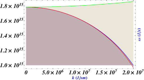
Figure 1: The figure shows the dispersion characteristic of the quantum Langmuir wave frequency $\omega$ versus the wave vector $k$, which is described by the equation (9). The green branch of dispersion is presented the classical high frequency Langmuir wave, the red and blue branches characterize the Coulomb exchange interactions and quantum Bohm potential influence, where $n_{0e}\simeq 10^{21}cm^{-3}$, $\eta=1$.

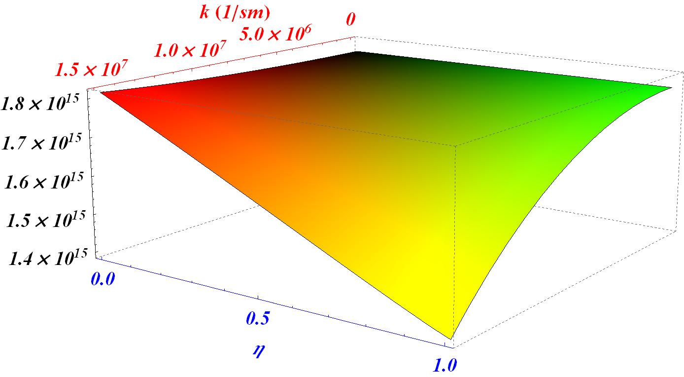
Figure 2: The figure shows the dispersion characteristic of the quantum Langmuir wave frequency $\omega$ as a function of the wave vector $k$ and the ratio of polarizability $\eta$, which is described by the equation (9). The Coulomb exchange interactions and quantum Bohm potential are taken into account and $n_{0e}\simeq 10^{21}cm^{-3}$.

$$\omega_{Le,3D}^{2}=\frac{4\pi e^{2}n_{0,3D}}{m_{e}}.$$ (8)

$$\omega^{2}=\omega_{Le,3D}^{2}-\zeta_{3D}\sqrt[3]{\frac{3}{\pi}}\frac{e^{2}}{m_{e}}\sqrt[3]{n_{0e}}k^{2}$$

$$+\vartheta_{3D}\frac{(3\pi^{2})^{2/3}\hbar^{2}n_{0e}^{2/3}}{3m_{e}^{2}}k^{2}+\frac{\hbar^{2}k^{4}}{4m_{e}^{2}},$$ (9)

where the dispersion of quantum Langmuir waves with the account of Coulomb exchange interactions (9) is presented at Fig. (1). In general case of of partially polarized system of particles with spin up and spin down, the dispersion of quantum Langmuir waves as a function of ratio of polarizability with account of Coulomb exchange interactions (9) is presented at Fig. (2).

We see that the first term in Eq. (9) is proportional to the electron equilibrium concentration $\sim n_{0e}$ and grows faster then the second term $\sim n_{0e}^{1/3}$. The third term has an intermediate rate of grow being proportional to $\sim n_{0e}^{2/3}.$ The Coulomb exchange interaction is larger than the Fermi pressure when $\sim n_{0e}\leq 10^{24}cm^{-3},$ this situation is realized in metals and semiconductors, but in the astrophysical objects like white drafts $\sim n_{0e}\leq 10^{28}cm^{-3},$ the Fermi pressure is larger than the Coulomb exchange interaction.

We have considered high frequency waves. Nest step is consideration of the low frequency excitations

$$\omega_{3D}(k)=kv_{s,3D}\sqrt{1-\frac{\zeta_{3D}}{\vartheta_{3D}}\frac{3}{4\pi}\sqrt[3]{\frac{3}{\pi}}\frac{\omega_{Le,3D}^{2}}{n_{0e,3D}^{2/3}v_{Fe,3D}^{2}}}\times$$

$$\times\frac{1}{\sqrt{1+(kr_{De,3D})^{2}\biggl{(}1-\frac{\zeta_{3D}}{\vartheta_{3D}}\frac{3}{4\pi}\sqrt[3]{\frac{3}{\pi}}\frac{\omega_{Le,3D}^{2}}{n_{0e,3D}^{2/3}v_{Fe,3D}^{2}}\biggr{)}}},$$ (10)

where $v_{s,3D}=\sqrt{m_{e}/m_{i}}\sqrt{\vartheta_{3D}}\cdot v_{Fe,3D}/3$ is the three dimensional velocity of sound, $r_{De,3D}=\sqrt{\vartheta_{3D}}v_{Fe,3D}/(3\omega_{Le,3D})$ is the Debye radius. In formula (9) and similar formulas below we extract contribution of the Fermi pressure. Hence formulas for ion-acoustic waves contains well-known contribution of the pressure multiplied by factor showing contribution of exchange interaction.

In the long wavelength limit we have

$$\omega(k)=kv_{s,3D}\sqrt{1-\frac{\zeta_{3D}}{\vartheta_{3D}}\frac{3}{4\pi}\sqrt[3]{\frac{3}{\pi}}\frac{\omega_{Le,3D}^{2}}{n_{0e,3D}^{2/3}v_{Fe,3D}^{2}}}.$$ (11)

In the short wavelength limit we find

$$\omega^{2}(k)=\omega_{Li,3D}^{2}.$$ (12)

IV Ion-acoustic waves in non-isothermal magnetized plasmas

Figure 3: The figure shows the dispersion characteristic of the long wavelength ion-acoustic wave frequency $\omega$ versus the wave vector $k$, which is described by the equation (14). The red mode shows the dispersion characteristic of the long wavelength ion-acoustic wave, where the thermal speed is defined by the Fermi pressure, the orange mode presents the Coulomb exchange interactions influence for $\eta=1$, the green mode for the case of partially polarized system $\eta=0.8$, the black mode for $\eta=0.5$ and the blue mode presents the Coulomb exchange interactions influence for $\eta=0.2$. System parameters are assumed to be as follows: $B_{0}\simeq 5\cdot 10^{5}$ G - the uniform magnetic field, $n_{0}\simeq 10^{18}$cm^-3 - the equilibrium density.

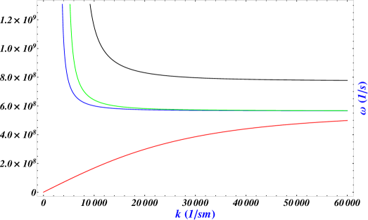
Figure 4: The figure shows the dispersion characteristic of the long wavelength ion-acoustic wave frequency $\omega$ versus the wave vector $k$, which is described by the equation (15). The red mode shows the dispersion characteristic of the long wavelength ion-acoustic wave, where the thermal speed is defined by the Fermi pressure and the blue mode presents the Coulomb exchange interactions influence for $\eta=1$, the green mode for $\eta=0.5$ and the black mode for $\eta=0.2$. System parameters are assumed to be as follows: $B_{0}\simeq 5\cdot 10^{5}$ G - the uniform magnetic field, $n_{0}\simeq 10^{18}$cm^-3 - the equilibrium density.

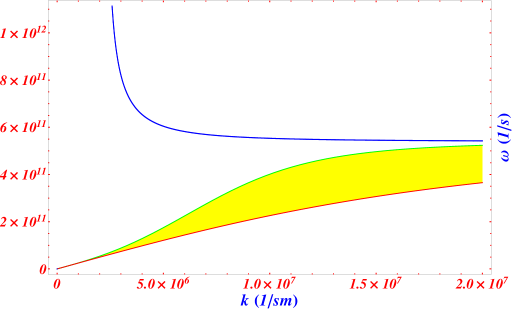
Figure 5: The figure shows the dispersion characteristic of the short wavelength quantum Langmuir wave frequency $\omega$ versus the wave vector k, which is described by the equation (9). The green mode shows the dispersion characteristic of quantum ion-acoustic waves which are described by equation (14), the red mode shows the dispersion characteristic of classic ion-acoustic waves which occur from (14) if the term proportional to  $\hbar^{2}$ is neglected. The blue mode shows the dispersion characteristic of the short wavelength wave where the Coulomb exchange interactions are dominate.

Lets discuss the ion-acoustic waves in non-isothermal magnetized plasmas with $T_{e}>>T_{i}\approx 0$ at $\Omega_{e}^{2}\gg\omega_{Li}^{2}\gg\Omega_{i}^{2}$ Kuzelev Ruhadze UFN1999 . In these conditions the ion-acoustic waves exist giving two branches of wave dispersion. One branch is at $\omega<\Omega_{i}$ and another one at $\omega>\Omega_{i}$.

Corresponding dispersion equation appears as

$$1-\frac{k_{\perp}^{2}\omega_{Li}^{2}}{k^{2}(\omega^{2}-\Omega_{i}^{2})}-\frac{k_{z}^{2}\omega_{Li}^{2}}{k^{2}\omega^{2}}+\frac{\omega_{Le}^{2}}{k^{2}v_{Te}^{2}}=0,$$ (13)

where $v_{Te}^{2}$ - is the thermal electron velocity. Using the approximation $\omega_{Li}^{2}\gg\Omega_{i}^{2}$ and $\theta\neq 0$ we find

$$\omega_{+}^{2}=\frac{\omega_{Li}^{2}+\Omega_{i}^{2}(1+\omega_{Li}^{2}/k^{2}v_{s}^{2})}{1+\omega_{Li}^{2}/k^{2}v_{s}^{2}},$$ (14)

and

$$\omega_{-}^{2}=\frac{\omega_{Li}^{2}\Omega_{i}^{2}\cos^{2}\theta}{\omega_{Li}^{2}+\Omega_{i}^{2}(1+\omega_{Li}^{2}/k^{2}v_{s}^{2})},$$ (15)

where

$$\upsilon^{2}_{s}=-\xi_{3D}\frac{e^{2}}{m_{i}}\sqrt[3]{\frac{3}{\pi}}\sqrt[3]{n_{0e}}$$

$$\qquad\qquad\qquad+\vartheta_{3D}\frac{(3\pi^{2})^{2/3}\hbar^{2}n_{oe}^{2/3}}{3m_{e}m_{i}}+\frac{\hbar^{2}k^{2}}{4m_{e}m_{i}}.$$ (16)

contains the Coulomb exchange interaction between electrons (the first term). The second term appears from the Fermi pressure. and the third term describes contribution of the quantum Bohm potential

Solutions of the equation (13) for the different ratio of polarizability are presented by two branches of the dispersion at Fig. (3), (4) and (5).

When the distribution of the wave is parallel to the background magnetic field $\theta=0$ the ion-acoustic modes have the form of

$$\omega^{2}=\Omega^{2}_{i}$$ (17)

and

$$\omega^{2}=\Biggl{(}-\xi_{3D}\frac{e^{2}}{m_{i}}\sqrt[3]{\frac{3}{\pi}}\sqrt[3]{n_{0e}}+\vartheta_{3D}\frac{(3\pi^{2})^{2/3}\hbar^{2}n_{oe}^{2/3}}{3m_{e}m_{i}}+\frac{\hbar^{2}k^{2}}{4m_{e}m_{i}}\Biggr{)}\times$$ (18)

$$\times\frac{\omega^{2}_{Li}k^{2}}{\omega^{2}_{Li}+k^{2}(-\xi_{3D}\frac{e^{2}}{m_{i}}\sqrt[3]{\frac{3}{\pi}}\sqrt[3]{n_{0e}}+\vartheta_{3D}\frac{(3\pi^{2})^{2/3}\hbar^{2}n_{oe}^{2/3}}{3m_{e}m_{i}}+\frac{\hbar^{2}k^{2}}{4m_{e}m_{i}})}$$

V The Trivelpiece-Gould waves

Trivelpiece-Gould wave Kuzelev Ruhadze UFN1999 , Tercas PP 08 is a longitudinal wave appearing along with the Langmuir wave at propagation of waves at an angle to external magnetic field $k_{x}\neq 0$ and $k_{z}\neq 0$. It is a low-frequency wave with $\omega\ll\mid\Omega_{e}\mid$. It exists at long wavelengths limit $\ll 1$, $k_{z}^{2}v_{Te}^{2}\ll\omega^{2}$. All of these conditions give the following dispersion equation

$$1-\frac{\omega_{Le}^{2}}{\omega^{2}}\frac{k_{z}^{2}}{k^{2}}+\frac{\omega_{Le}^{2}}{k^{2}v_{Te}^{2}}\frac{k_{x}^{2}v_{Te}^{2}}{\Omega_{e}^{2}}=0$$ (19)

Dispersion dependence of the Trivelpiece-Gould wave in the classical magnetic field appears as Tercas PP 08

$$\omega^{2}=\frac{\omega_{Le}^{2}\cos^{2}\theta}{1+\frac{\omega_{Le}^{2}\sin^{2}\theta}{\Omega_{e}^{2}}}.$$ (20)

It looks like thermal velocity does not affect this spectrum. If it is correct we can mention that the exchange interaction does not influence it either. In the quantum external magnetic field the thermal velocity effect might be important. This corresponds to a regime of very strong magnetic field in which the external field strength approaches or exceeds the quantum critical magnetic field, $B_{0}\geq 4.4\cdot 10^{13}$ G. Evidently, since $\hbar\Omega_{e}>>T_{e}$ there must exist the frequency

$$\omega^{2}=\frac{m_{e}\Omega_{e}\tan^{2}\theta}{\hbar}\times$$ (21)

$$\times\Biggl{(}-\xi_{3D}\frac{e^{2}}{m_{e}}\sqrt[3]{\frac{3}{\pi}}\sqrt[3]{n_{0e}}+\vartheta_{3D}\frac{(3\pi^{2})^{2/3}\hbar^{2}n_{oe}^{2/3}}{3m_{e}^{2}}+\frac{\hbar^{2}k^{2}}{4m_{e}^{2}}\Biggr{)}.$$

VI The longitudinal low-frequency ion-acoustic waves in magnetized plasmas

In absence of external magnetic field longitudinal oscillations exists in electron-ion plasmas with hot electrons and cold ions Kuzelev Ruhadze UFN1999 . They are weakly damping ion-acoustic oscillations Ahiezer . Dispersion of these waves is

$$\omega_{s}(\textbf{k})=\frac{kv_{s}}{\sqrt{1+k^{2}r_{D}^{2}}},$$ (22)

where $r_{D}=\sqrt{T_{e}/4\pi e^{2}n_{0}}$ is the Debay radius, $v_{s}=\sqrt{T_{e}/m_{i}}$. This solution corresponds to phase velocities of waves, which are intermediate in compare with other parameters of plasmas $v_{i}\ll\omega/k\ll v_{e}$ with the thermal velocities of electrons $v_{e}=\sqrt{T_{e}/m_{e}}$ and ions $v_{i}=\sqrt{T_{i}/m_{i}}$.

If equilibrium state of a medium reveals distribution of electrons with non-zero magnetization, as it happens in ferromagnetic domains, the Coulomb exchange interaction gives considerable contribution in spectrum of the longitudinal waves Andreev Exchange 14 .

It is well-known that an external magnetic field affects the ion-acoustic waves at $\omega_{s}(\textbf{k})\leq\Omega_{i}$ and $k\rho_{i}\leq 1$. Presence of external magnetic field creates or increases difference in occupation of spin-up and spin-down states. Consequently, account of the Coulomb exchange interaction in magnetized plasmas is even more important than in plasmas with no external magnetic field.

Under conditions $v_{i}\ll\mid\omega/k_{\parallel}\mid\ll v_{e}$ we find the following dispersion equation for the longitudinal low-frequency ion-acoustic waves

$$1+\frac{\omega_{Le}^{2}}{\Omega_{e}^{2}}+\frac{\omega_{Li}^{2}}{k^{2}v_{s}^{2}}-\frac{\omega_{Li}^{2}}{\omega^{2}}\cos^{2}\theta-\frac{\omega_{Li}^{2}}{\omega^{2}-\Omega_{i}^{2}}\sin^{2}\theta=0,$$ (23)

where $\Omega_{a}=\frac{q_{a}B_{0}}{m_{a}c}$ - are the the electron or ion cyclotron frequency.

Increasing of the Coulomb exchange interaction in compare with the Fermi pressure can break condition of the ion-acoustic wave existence $v_{i}\ll\mid\omega/k_{\parallel}\mid\ll v_{e}$.

Getting into account the fact that in the problem under consideration the second term in equation (23) much smaller than the third term we find next solution

$$\omega^{2}(k,\theta)=\frac{1}{2}(\omega_{s}^{2}+\Omega_{i}^{2})\pm\frac{1}{2}\sqrt{(\omega_{s}^{2}+\Omega_{i}^{2})^{2}-4\omega_{s}^{2}\Omega_{i}^{2}\cos^{2}\theta}.$$ (24)

We have also neglected small anisotropic terms.

In presence of an external magnetic field, there are two longitudinal low-frequency oscillations instead of the ion-acoustic wave.

At $k\rightarrow 0$ we find from formula (24)

$$\omega(k,\theta)=kv_{s}\cos\theta,$$ (25)

and

$$\omega(k,\theta)=\Omega_{i}\biggl{(}1+\frac{k^{2}v_{s}^{2}\sin^{2}\theta}{2\Omega_{i}^{2}}\biggr{)}.$$ (26)

The condition for instability is thus that the negative term of $v_{s}^{2}$ dominates over all the others. When the Coulomb exchange interactions is larger than Fermi pressure $n_{0}\leq 10^{23}sm^{-3}$, the solution (25) is instability. The solution (26) is presented at Fig. (6) as a function of $\eta$.

In opposite limit of small wavelengths $k\rightarrow\infty$, or in other terms $kr_{D}\gg 1$, from formula (24) we obtain

$$\omega_{\pm}^{2}(\theta)=\frac{1}{2}(\omega_{Li}^{2}+\Omega_{i}^{2})\pm\frac{1}{2}\sqrt{(\omega_{Li}^{2}+\Omega_{i}^{2})^{2}-4\omega_{Li}^{2}\Omega_{i}^{2}\cos^{2}\theta}.$$ (27)

Formula (27) is obtained at $k^{2}\rho_{i}^{2}\ll 1$. It can be applied at $\frac{T_{i}}{T_{e}}\frac{\omega_{Li}^{2}}{\Omega_{i}^{2}}\ll 1$. Under condition $\omega_{Li}\gg\Omega_{i}$ formula (27) does not work. Formula (24) can be applied in the long wavelength limit $kr_{D}\ll 1$ if condition $\omega_{Li}\gg\Omega_{i}$ is satisfied.

Figure 6: The figure shows the dispersion characteristic of the low-frequency oscillations in the long wavelengths $k\rightarrow\infty$ limit, which is described by the equation (26), $n_{0}\simeq 10^{18}sm^{-3}$, $B_{0}=5\cdot 10^{4}$ G. The red branch characterizes the total polarized system $\eta=1$, the blue mode $\eta=0.5$ and green mode $\eta=0.2$ present the dispersion properties of partially polarized systems.

Under conditions $kv_{s}\gg\Omega_{i}$ and $kr_{D}\ll 1$, we obtain the following solutions from formula (24)

$$\omega(k)=kv_{s},$$ (28)

and

$$\omega(k,\theta)=\Omega_{i}\cos\theta.$$ (29)

The Coulomb exchange interaction in (28) is larger than the Fermi pressure when $\sim n_{0e}\leq 10^{25}cm^{-3},$ this situation is realized in metals and semiconductors, but in the astrophysical objects like white drafts $\sim n_{0e}\leq 10^{28}cm^{-3},$ the Fermi pressure is larger than the Coulomb exchange interaction.

At $k\rightarrow 0$ ($kv_{s}\ll\Omega_{i}$) larger of solutions (24) presented by formula (28) getting to $\Omega_{i}$.

We can also present corresponding refractive index

$$N^{2}=\frac{c^{2}}{\upsilon_{s}^{2}}\frac{\omega^{2}-\Omega_{i}^{2}}{\omega^{2}-\Omega_{i}^{2}\cos^{2}\theta}.$$ (30)

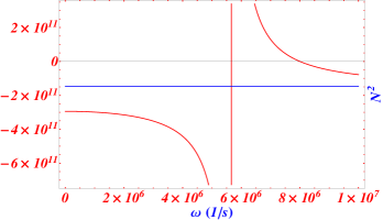
Figure 7: The figure shows the corresponding classical refractive index (30) in the limit of the long wavelength limit $kr_{D}\ll 1$, where the Coulomb exchange interactions are dominate $\gamma_{ex}^{2}>\upsilon_{Fe}^{2}$. System parameters are assumed to be as follows: $n_{0}\simeq 10^{15}sm^{-3}$, $B_{0}=5\cdot 10^{3}$ G. The blue branch is the index $c^{2}/\gamma_{ex}^{2}.$

Figure 8: The figure shows the dispersion characteristic of the slow and fast magneto-sonic waves, which is described by the equation (24) in the long wavelength limit $kr_{D}\ll 1$, $n_{0}\simeq 10^{23}sm^{-3}$, $B_{0}=5\cdot 10^{4}$ G. The red branch characterizes the dispersion of total polarized system $\eta=1$, the blue mode $\eta=0.3$ and green mode $\eta=0.2$ present the dispersion properties of partially polarized systems.

Using the definition (16) the Coulomb exchange pressure can be important for the slow and fast magneto-sonic wave, see Fig. (8).

VII The low-frequency electromagnetic oscillations in the magnetized plasma

Here we discuss low-frequencies electromagnetic waves at $T_{e}\gg T_{i}$ under influence of the Coulomb exchange interaction.

Dispersion equation existing in the case under consideration is rather huge. Thus we do not present it here. Nevertheless, we present description of limit cases. In low frequency limit, it corresponds to the long wavelength limit $k\rightarrow 0$, we have the dispersion of the slow and fast magneto-sonic waves

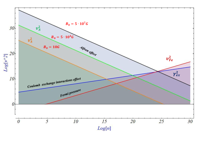
Figure 9: A figure illustrating regions of importance in parameter space for various quantum plasma effects of the longitudinal wave propagating perpendicular to the external magnetic field (36). The orange, green and black branches describe the Alfv en regime.

$$\omega=kv_{A}\cos\theta$$ (31)

and

$$\omega=kv_{\pm},$$ (32)

where the Alfven velocity is

$$v_{A}=c\frac{\Omega_{i}}{\omega_{Li}}=\frac{B_{0}}{\sqrt{4\pi n_{0}m_{i}}}$$ (33)

and

$$v_{\pm}^{2}=\frac{1}{2}(v_{A}^{2}+v_{s}^{2})\pm\frac{1}{2}\sqrt{(v_{A}^{2}+v_{s}^{2})^{2}-4v_{A}^{2}v_{s}^{2}\cos^{2}\theta}$$ (34)

For the wave propagating parallel to the external magnetic field $\cos\theta\simeq 0$ the dispersion low (32) has the form

$$\omega_{\pm}=k\begin{cases}v_{A},\\ v_{s}.\end{cases}$$ (35)

Lets consider the longitudinal wave propagating perpendicular to the external magnetic field. The dispersion low (32) takes the form

$$\omega^{2}=k^{2}\Biggl{(}\upsilon^{2}_{A}+\upsilon^{2}_{i}-\xi_{3D}\frac{e^{2}}{m_{i}}\sqrt[3]{\frac{3}{\pi}}\sqrt[3]{n_{0e}}$$ (36)

$$\qquad\qquad\qquad+\vartheta_{3D}\frac{(3\pi^{2})^{2/3}\hbar^{2}n_{oe}^{2/3}}{3m_{e}m_{i}}+\frac{\hbar^{2}k^{2}}{4m_{e}m_{i}}\Biggr{)},$$

$$\vartheta_{3D}=\frac{1}{2}[(1+\eta)^{5/3}+(1-\eta)^{5/3}],$$ (37)

$$\xi_{3D}=[(1+\eta)^{4/3}-(1-\eta)^{4/3}].$$

The figure (9) shows regions of importance in parameter space for various quantum plasma effects $\eta=1$. The Fermi-pressure $\sim\upsilon^{2}_{Fe}\sim n_{oe}^{2/3}$ becomes important when the Fermi temperature approaches the thermodynamic temperature, when the plasma concentration $n_{0}\geq 10^{25}$cm^-3. The Alfv en mode described by the first term $\upsilon^{2}_{A}$ on the right side of (36). The effects due to the magnetic pressure depend on the magnetic field strength $\upsilon^{2}_{A}\sim n_{0}^{-1}$. The magnetic pressure effects can be important in regimes of $n_{0}\leq 10^{20}$cm^-3 and external magnetic field $B_{0}\simeq 5\cdot 10^{4}$G. The quantum regime correspond to lower temperatures. The Coulomb exchange interactions proportional to $\sim\gamma^{2}_{ex}\sim n_{0e}$ can be important in regimes of $10^{20}\leq n_{0}\leq 10^{24}$cm^-3. The Coulomb exchange force does not provide a stabilizing mechanism. The exchange pressure $\sim\gamma^{2}_{ex}=\xi_{3D}\sqrt[3]{\frac{3}{\pi}}\sqrt[3]{n_{0e}}e^{2}/m_{i}$ is the negative pressure term and therefore the source of the instability. But for the high magnitude magnetic field $B_{0}\sim 10^{7}G$, the instability is stabilized.

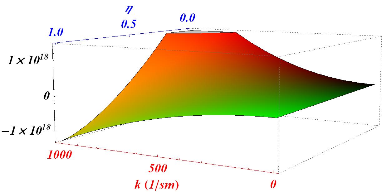
Figure 10: The 3D figure shows the dispersion characteristic of the magneto-sonic waves, which is described by the equation (36), where the exchange effects are taken into account. The 3D figure represents the wave frequency $\omega^{2}(k,\eta)$ as a function of the wave vector $k$ and the ratio of polarizability $\eta$. The Coulomb exchange interactions and quantum Bohm potential are taken into account and $n_{0e}\simeq 10^{23}cm^{-3}$.

Let us consider the small wavelength limit $k\rightarrow\infty$. In this regime the refractive index and frequency of smallest of three solutions appear as

$$N^{2}=(2N_{A}^{2}+N_{s}^{2}\sin^{2}\theta)\frac{\Omega_{i}^{2}}{\Omega_{i}^{2}\cos^{2}\theta-\omega^{2}},$$ (38)

and

$$\omega(k,\theta)=\Omega_{i}\cos\theta\times$$ (39)

$$\times\Biggl{[}1-\frac{\Biggl{[}2\Biggl{(}-\xi_{3D}\frac{e^{2}}{m_{i}}\sqrt[3]{\frac{3}{\pi}}\sqrt[3]{n_{0e}}+\frac{\hbar^{2}k^{2}}{4m_{e}m_{i}}\Biggr{)}+\sin^{2}\theta v_{A}^{2}\Biggr{]}\Omega_{i}^{2}}{2k^{2}v_{A}^{2}\Biggl{(}-\xi_{3D}\frac{e^{2}}{m_{i}}\sqrt[3]{\frac{3}{\pi}}\sqrt[3]{n_{0e}}+\frac{\hbar^{2}k^{2}}{4m_{e}m_{i}}\Biggr{)}}\Biggr{]},$$

where $N_{A}=c/v_{A}$, $N_{s}=c/v_{s}$. The dispersion of quantum slow magneto-sonic waves in the small wavelength limit $k\rightarrow\infty$ is presented at Fig. (11).

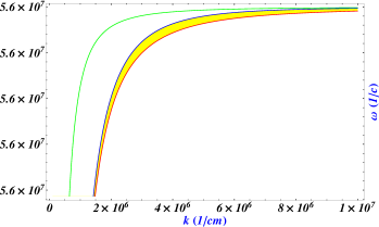
Figure 11: The figure shows the dispersion characteristic of the slow magneto-sonic waves, which is described by the equation (39) in the small wavelength limit $k\rightarrow\infty$, where the exchange effects are taken into account. The red branch of dispersion represents the classical low, the blue branch include the dispersion characteristic of quantum slow magneto-sonic waves which occurs due to Bohm quantum potential and the green mode takes account of Coulomb exchange interactions.

VIII Conclusions

We have briefly described quantum hydrodynamic model for the magnetized quantum plasmas. In our work we consider the electron-electron and ion-ion Coulomb exchange interactions. Using QHD equations with Coulomb exchange force field we analyzed elementary excitations in various physical systems in a linear approximation. We investigated the dispersion properties of the ion-acoustic waves in non-isothermal magnetized plasmas, the Trivelpiece-Gould waves, the longitudinal low-frequency ion-acoustic waves, the magneto-sonic waves, high-frequency and low-frequency electron sound tracing contribution of the exchange interaction. We described the different regimes and showed that the exchanges interactions can lead to instability.

References

(1) L. S. Kuz’menkov and S. G. Maksimov, Teor. i Mat. Fiz.,
118 287 (1999) [Theoretical and Mathematical Physics 118 227 (1999)].
(2) L. S. Kuz’menkov, S. G. Maksimov, and V. V. Fedoseev, Theor.
Math. Fiz. 126 258 (2001) [Theoretical and Mathematical
Physics, 126 212 (2001)].
(3) P. A. Andreev, L. S. Kuz’menkov, Phys. Rev. A 78, 053624 (2008).
(4) P. A. Andreev, arXiv:1403.6075.
(5) L. S. Kuz’menkov, S. G. Maksimov, and V. V. Fedoseev, Russian Phys. Jour. 43, 718 (2000).
(6) L. S. Kuz’menkov, S. G. Maksimov, and V. V. Fedoseev, Theor.
Math. Fiz. 126 136 (2001) [Theoretical and Mathematical
Physics, 126 110 (2001)].
(7) F. Haas, G. Manfredi, M. Feix, Phys. Rev. E 62,
2763(2000).
(8) G. Manfredi and F. Haas, Phys. Rev. B 64, 075316 (2001).
(9) P. K. Shukla, B. Eliasson, Phys. Usp. 53, 51 (2010).
(10) P. K. Shukla, B. Eliasson, Rev. Mod. Phys. 83, 885 (2011).
(11) M. Marklund and G. Brodin,
Phys. Rev. Lett. 98, 025001 (2007).
(12) G. Brodin and M. Marklund, New J. Phys, 9, 277
(2007).
(13) P. A. Andreev, L. S. Kuz’menkov,
Physics of Atomic Nuclei 71, N.10, 1724 (2008).
(14) P. A. Andreev, L. S. Kuz’menkov, Int. J. Mod. Phys. B 26 1250186 (2012).
(15) P. A. Andreev and L. S. Kuzmenkov, PIERS Proceedings, Marrakesh, Morocco, March
20-23, 1047 (2011).
(16) M. Iv. Trukhanova, Progr. Theor. Exp. Phys. 2013, 111I01 (2013).
(17) M. I. Trukhanova, Eur. Phys. J. D 67, Issue 2, 32 (2013).
(18) T. Koide, Phys. Rev. C 87, 034902 (2013).
(19) P. A. Andreev and L. S. Kuz’menkov, Russian Phys. Jour. 50, 1251 (2007).
(20) P. A. Andreev, L. S. Kuzmenkov, M. I. Trukhanova, Phys. Rev. B 84, 245401 (2011).
(21) J. Zamanian, M. Marklund, G. Brodin, Phys. Rev. E 88, 063105 (2013).
(22) J. Zamanian, M. Marklund, G. Brodin, arXiv: 1402.7240 (2014).
(23) Woo-Pyo Hong and Young-Dae Jung, Phys. Scr. 89, 065601 (2014).
(24) Young-Dae Jung and M. Akbari-Moghanjoughi, Phys. Plasmas 21, 032108 (2014).
(25) M. V. Kuzelev, A. A. Rukhadze, Phys. Usp. 42, 603 (1999).
(26) H. Tercas, J. T. Mendon a, and P. K. Shukla, Phys. Plasmas 15, 072109 (2008).
(27) A. I. Akhiezer, I. A. Akhiezer, R. V. Polovin, et al.,
Plasma Electrodynamics (Nauka, Moscow, 1974) [in
Russian].