Abstract

Non-local closures allow kinetic effects on parallel transport to be included in fluid simulations. This is especially important in the scrape-off layer, but to be useful there the non-local model requires consistent kinetic boundary conditions at the sheath. A non-local closure scheme based on solution of a kinetic equation using a diagonalized moment expansion has been previously reported. We derive a method for imposing kinetic boundary conditions in this scheme and discuss their implementation in BOUT++. To make it feasible to implement the boundary conditions in the code, we are lead to transform the non-local model to a different moment basis, better adapted to describe parallel dynamics. The new basis has the additional benefit of enabling substantial optimization of the closure calculation, resulting in an $\mathcal{O}(10)$ speedup of the non-local code.

1 Introduction

Kinetic effects on parallel dynamics may be important in cases where we would otherwise like to use fluid models: in the scrape-off layer (SOL), as the collision length is often comparable to the parallel connection length; or if, for example, we wish to include some Landau damping physics. To avoid the computational expense of moving to fully kinetic simulations, we can introduce these kinetic effects into fluid models through non-local closures that solve (approximately) the electron kinetic problem in quasi-steady-state. Here we discuss some new developments to the non-local closure model implemented in BOUT++[1], first described in [2] and based on the method of [3], in which the 1d kinetic equation is solved using a moment expansion truncated at very high order (up to several hundred moments).

In order for a non-local closure to be useful in the SOL it requires boundary conditions at the sheath edge. These must go beyond just the fluid velocity (Bohm condition) and heat transmission to specify completely the boundary conditions for the kinetic equation being solved. We describe below (Section 4) a method for and implementation of such kinetic boundary conditions in the simplest case, neglecting secondary electron emission.

The kinetic boundary condition depends only on the parallel velocity, so the boundary equations are separable. It also introduces a sharp feature in the distribution function (due the tail absorbed by the wall being removed), and therefore requires a large number of moments, but only in the parallel velocity part of the distribution function. In the previous implementations of this model the moment expansion used basis functions depending on pitch angle (Legendre polynomials) and speed (associated Laguerre polynomials). In order to achieve a certain resolution in the parallel velocity, both of these expansions must be taken to the same order so that we have $\mathcal{O}(n^{2})$ moments for some $n$. In order to take advantage of the separation into parallel and perpendicular velocity parts we here reformulate the closures on a new basis better adapted to the problem at hand, namely an expansion in parallel velocity (Hermite polynomials) and perpendicular speed (Laguerre polynomials). In order to resolve the same features in the parallel velocity we still need $\mathcal{O}(n)$ components in the Hermite expansion, but we can now set the order of the Laguerre part independently, allowing the total number of moments to be $\mathcal{O}(n\times m)$ with $m\ll n$. The transformation to the new basis is presented in Section 2.

However, the new basis is not only useful for the boundary conditions. Since we are solving a 1d kinetic problem, the separation between parallel and perpendicular velocities is generally a useful one to make; although the collision operator does couple the parallel and perpendicular velocity parts, if collisions are the dominant process we return to the local limit exactly (regardless of the order of the truncation) and so we need to optimize only for the case when they are not too strongly coupled. Thus, as we show for the examples in Section 3, we can make substantial performance gains for little loss in accuracy by using the new basis and choosing the orders of the Hermite and Laguerre expansions appropriately.

2 Choice of moment basis

Previous work on this non-local model[3, 2] used a moment basis of Legendre polynomials in pitch angle, $P_{l}(\cos\theta)$, and associated Laguerre polynomials in speed, $L_{k}^{(l+1/2)}(s^{2})$ (the ‘old basis’). Throughout we use $\vec{s}=\vec{v}/v_{T}$ (correspondingly $s=v/v_{T}$, $s_{\|}=v_{\|}/vT$, $s_{\perp}=v_{\perp}/v_{T}$, $s_{\text{sheath}}=v_{\text{sheath}}/v_{T}$) for velocities normalized by the thermal speed, $v_{T}=\sqrt{\frac{2T}{m}}$. The old basis is well-adapted for the calculation of the collision matrix[4] which, being isotropic, is block-diagonal in $l$. However, the calculation of parallel closures is highly anisotropic; in this case a basis in which parallel velocity, $v_{\|}$, and perpendicular velocity, $v_{\perp}$, are separable is more natural and convenient (the ‘new basis’). This is especially true for the calculation of sheath boundary conditions (section 4), which originally motivated the change.

To choose the basis functions explicitly, we identify the appropriate sets of orthogonal polynomials. For the parallel velocity we take the Hermite polynomials $H_{p}(s_{\|})$ which are the complete set of orthogonal polynomials on the interval $(-\infty,\infty)$ with weight function $e^{-s_{\|}^{2}}$. For the perpendicular velocity we take the Laguerre polynomials $L_{j}(x)$ which are the complete set of orthogonal polynomials on the interval $[0,\infty)$ with weight function $e^{-x}$.

Since $\cos\theta=\frac{s_{\|}}{s}$, $s^{2}=s_{\|}^{2}+s_{\perp}^{2}$ and the $P_{l}$ are odd or even functions according as $l$ is odd or even, $s^{l}P_{l}(\cos\theta)$ and $L_{k}^{(l+1/2)}(s^{2})$ are polynomials in $s_{\|}$ and $s_{\perp}^{2}$. They are therefore given by a finite sum of the new basis functions,

$$s^{l}P_{l}(\cos\theta)L_{k}^{(l+1/2)}(s^{2}) =\sum_{p=0}^{p_{\text{max}}}\sum_{j=0}^{j_{\text{max}}}T_{lk}^{pj}H_{p}(s_{\|})L_{j}(s_{\perp}^{2})=\sum_{p=0}^{p_{\text{max}}}T_{lk}^{p\hat{j}}H_{p}(s_{\|})L_{\hat{j}}(s_{\perp}^{2})$$ (1)

with $p_{\text{max}}=l+2k$, $\hat{j}=\frac{l-p}{2}+k$. Similarly

$$H_{p}(s_{\|})L_{j}(s_{\perp}^{2})= \sum_{l=0}^{l_{\text{max}}}\sum_{k=0}^{k_{\text{max}}}\left(T^{-1}\right)_{pj}^{lk}s^{l}P_{l}(\cos\theta)L_{k}^{(l+1/2)}(s^{2})=\sum_{l=0}^{l_{\text{max}}}\left(T^{-1}\right)_{pj}^{l\hat{k}}s^{l}P_{l}(\cos\theta)L_{\hat{k}}^{(l+1/2)}(s^{2})$$ (2)

with $l_{\text{max}}=p+2j$, $\hat{k}=\frac{p-l}{2}+j$. To compute the collision matrix in the new basis exactly up to some order, we may transform the result in the old basis (${\displaystyle C_{p^{\prime}j^{\prime}}^{pj}=\sum_{l,l^{\prime}=0}^{l_{\text{max}}}\sum_{k,k^{\prime}=0}^{k_{\text{max}}}T_{lk}^{pj}C_{l^{\prime}k^{\prime}}^{lk}\left(T^{-1}\right)_{p^{\prime}j^{\prime}}^{l^{\prime}k^{\prime}}}$), with the collision matrix in the old basis only being required at finite order.

We can now write the kinetic equation in the new moment basis, where the moments are defined as ${\displaystyle n^{pj}=\frac{1}{2^{p}p!}}\int d^{3}v\,H_{p}(s_{\|})L_{j}(s_{\perp}^{2})f(\vec{v})$ and using the dimensionless length $z$ defined by $\frac{\partial\ell}{\partial z}=\lambda_{C}$,

$$v_{\|}\frac{\partial\delta f_{e}}{\partial\ell} =C\!\left(f_{e}^{(0)}\!+\!\delta f_{e}\right)-v_{\|}\frac{\partial\langle f_{e}^{(0)}\rangle}{\partial\ell}$$

$$\rightarrow\Psi_{p^{\prime},j^{\prime}}^{p,j}\frac{\partial n^{p^{\prime},j^{\prime}}}{\partial z} =C_{p^{\prime},j^{\prime}}^{p,j}n^{p^{\prime},j^{\prime}}+g^{p,j}$$ (3)

The moments of the free-streaming operator are straightforward to compute in the new basis

$$\Psi_{p^{\prime},j^{\prime}}^{p,j} \equiv\int d^{3}v\,H_{p}(s_{\|})L_{j}(s_{\perp}^{2})\sum_{p^{\prime},j^{\prime}}\frac{1}{\pi^{3/2}v_{T}^{3}}e^{-s^{2}}s_{\|}H_{p^{\prime}}(s_{\|})L_{j^{\prime}}(s_{\perp}^{2})$$

$$=2^{p}p!\left(\frac{1}{2}\delta_{p,p^{\prime}+1}+p^{\prime}\delta_{p,p^{\prime}-1}\right)\delta_{j,j^{\prime}}$$ (4)

Having found the coefficients of the moment equations we can, as before[2], diagonalize the system by going to an eigenvector basis and compute the closures as sums of integrals.

There is one slight complication. To compute the closures, we must remove from the system the equations for density, fluid velocity and temperature (which are solved dynamically). However, the moment corresponding to the temperature in the new basis is a linear combination of the $(p=2,j=0)$ and $(p=0,j=1)$ moments, so we must apply a further transformation to this pair of moments to remove the temperature part from the closures. We call this transformation $R$, and solve for the set of moments $n_{*}^{pj}=R_{p^{\prime}j^{\prime}}^{pj}n^{p^{\prime}j^{\prime}}$. $R$ differs from the identity only in four components, which are

$$\left(\begin{array}[]{cc}R_{0,1}^{0,1}&R_{2,0}^{0,1}\\ R_{0,1}^{2,0}&R_{2,0}^{2,0}\end{array}\right) =\left(\begin{array}[]{cc}\frac{1}{2}&-1\\ \frac{1}{3}&\frac{4}{3}\end{array}\right)$$ (9)

3 Comparison of bases

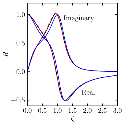
Figure 1: Response function for Hammett-Perkins closure (black), old basis with $30\times 30$ moments (red, dashed) and new basis with $30\times 2$ moments (blue)

Landau damping is an interesting test case for these closures because we have a known collisionless limit from the results of Hammett & Perkins[5]. It is possible to reproduce this collisionless limit by replacing the Hammett-Perkins expression for the heat-flux with the result from the non-local closures being discussed here and taking a sufficiently small (but non-zero) collisionality. To match the collisionless limit using the old basis requires $30\times 30$ moments for convergence. In the new basis, however, we have the advantage of being able to much reduce the number of moments; using only $30\times 2$ moments gives only a small loss in accuracy, as shown in Figure 1. Here and below we describe the number of moments in particular cases as pairs of numbers: (order of Legendre expansion)$\times$(order of associated Laguerre expansion) for the old basis and (order of Hermite expansion)$\times$(order of Laguerre expansion) for the new basis.

The decrease in the number of moments needed for convergence represents a significant gain for the performance of the code. To illustrate this we consider the drift-wave instability test-case, previously discussed in [6] but here with the electron parallel viscosity included. Convergence in the old basis requires $20\times 20$ moments, while in the new basis it requires only $20\times 2$; the total run time (for otherwise identical simulations) reduces from 106 cpu-hours to 11 cpu-hours. The simulations were run on a 4-core desktop machine, using a $32\times 32$ grid. The perturbation is seeded with a wavenumber $k_{\|}=8.15\times\frac{2\pi}{\lambda_{C}}$ so that we consider a low collisionality case. Figure 3 shows that convergence can be achieved for a much smaller number of moments using the new basis. The performance gain is demonstrated by Figure 3 where we see that the total run time for the simulations is directly proportional to the number of moments used, as the calculation of the closures dominates the computation time here (although in a typical three-dimensional simulation there would be other computationally intensive operations, such as Laplacian inversion, that might be comparable in computational time).

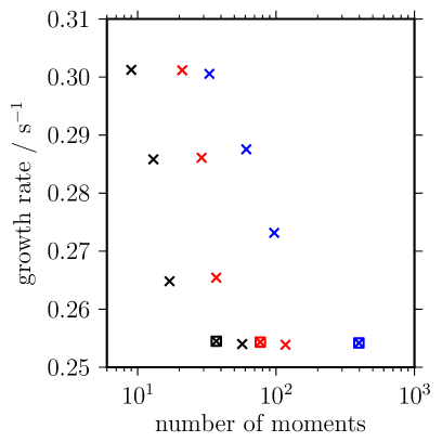
Figure 2: Convergence of drift instability simulation, growth rates for various numbers of moments: new basis $n\times 2$ (black), $n\times 4$ (red) and old basis (blue)

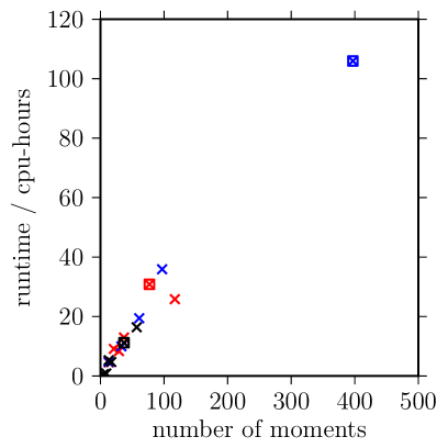
Figure 3: Run times for drift-wave simulation: new basis 2 (black), $n\times 4$ (red) and old basis (blue). Squares mark the smallest well converged simulations (see Figure 3)

4 Sheath boundary conditions

Calculation of correct sheath boundary conditions is much more complicated for the non-local model than for simple fluid models, not least because boundary conditions are required for several hundred moments rather than just a few. To derive boundary conditions for the non-local model we start from the simplest possible kinetic sheath boundary condition (with no secondary electron emission). Considering the sheath where outgoing $v_{\|}$ is positive

$$f_{\text{sheath}}(v_{\|},v_{\perp}) =\begin{cases}f_{+}(v_{\|},v_{\perp})&v_{\|}>0\\ f_{+}(-v_{\|},v_{\perp})&-v_{\text{sheath}}<v_{\|}<0\\ 0&v_{\|}<-v_{\text{sheath}}\end{cases}$$ (10)

where $v_{\text{sheath}}=\sqrt{-\frac{2e\phi_{\text{sheath}}}{m_{e}}}$ is the speed needed to cross the sheath potential. As this boundary condition is independent of $v_{\perp}$, the calculation is much cleaner in the new basis, since the expansion in $L_{j}(s_{\perp}^{2})$ is trivial everywhere.

First we translate this boundary condition into the moment representation.

$$n^{p,j} \equiv\frac{1}{2^{p}p!}\int d^{3}v\,H_{p}(s_{\|})L_{j}(v_{\perp}^{2})f(v_{\|},v_{\perp})$$

$$2^{p}p!\left.n^{p,j}\right|_{\text{sheath}} =\int d^{2}v_{\perp}\int_{0}^{\infty}dv_{\|}\,H_{p}(s_{\|})L_{j}(s_{\perp}^{2})f_{+}(v_{\|},v_{\perp})$$

$$\quad+\int d^{2}v_{\perp}\int_{-s_{\text{sheath}}}^{0}dv_{\|}\,H_{p}(s_{\|})L_{j}(s_{\perp}^{2})f_{+}(-v_{\|},v_{\perp})$$

$$=\begin{cases}\begin{array}[]{l}2\int d^{2}v_{\perp}\int_{0}^{\infty}dv_{\|}\,H_{p}(s_{\|})L_{j}(s_{\perp}^{2})f_{+}(v_{\|},v_{\perp})\\ -\int d^{2}v_{\perp}\int_{s_{\text{sheath}}}^{\infty}dv_{\|}\,H_{p}(s_{\|})L_{j}(s_{\perp}^{2})f_{+}(v_{\|},v_{\perp})\end{array}&p\text{ even}\\ \int d^{2}v_{\perp}\int_{s_{\text{sheath}}}^{\infty}dv_{\|}\,H_{p}(s_{\|})L_{j}(s_{\perp}^{2})f_{+}(v_{\|},v_{\perp})&p\text{ odd}\end{cases}$$ (11)

as $H_{p}(-v_{\|})=(-1)^{p}H_{p}(v_{\|})$. Since $f_{+}(v_{\|},v_{\perp})\equiv f(v_{\|},v_{\perp})$ for $v_{\|}>0$ we can expand $f_{+}$ in moments

$$\left.n^{p,j}\right|_{\text{sheath}} =\begin{cases}n^{p,j}+\sum_{p^{\prime}}\left(2X_{p^{\prime}}^{p}n^{(2p^{\prime}+1),j}-\beta_{p}^{p^{\prime}}n^{(2p^{\prime}+1),j}-\gamma_{p^{\prime}}^{p}n^{2p^{\prime},j}\right)&p\text{ even}\\ \sum_{p^{\prime}}\left(\alpha_{p^{\prime}}^{p}n^{(2p^{\prime}+1),j}+\beta_{p^{\prime}}^{p}n^{2p^{\prime},j}\right)&p\text{ odd}\end{cases}$$ (12)

defining

$$X_{p^{\prime}}^{p} =\frac{1}{2^{p}p!}\int_{0}^{\infty}ds_{\|}\,H_{p}(s_{\|})H_{(2p^{\prime}+1)}(s_{\|})e^{-s_{\|}^{2}}$$

$$\alpha_{p^{\prime}}^{p} =\frac{1}{2^{p}p!}\int_{s_{\text{sheath}}}^{\infty}ds_{\|}\,H_{(2p+1)}(s_{\|})H_{(2p^{\prime}+1)}(s_{\|})e^{-s_{\|}^{2}}$$

$$\beta_{p^{\prime}}^{p} =\frac{1}{2^{p}p!}\int_{s_{\text{sheath}}}^{\infty}ds_{\|}\,H_{(2p+1)}(s_{\|})H_{2p^{\prime}}(s_{\|})e^{-s_{\|}^{2}}$$

$$\gamma_{p^{\prime}}^{p} =\frac{1}{2^{p}p!}\int_{s_{\text{sheath}}}^{\infty}ds_{\|}\,H_{2p}(s_{\|})H_{2p^{\prime}}(s_{\|})e^{-s_{\|}^{2}}$$ (13)

We could use either relation in (12) to determine the odd-$p$ moments in terms of the even-$p$ moments or vice versa. They must be equivalent (before truncation) but the odd-$p$ version is simpler, so we use that.

Finally, the boundary condition that we want is on the eigenvector-basis moments. We need to determine the positive-eigenvalue (outgoing) moments (and the fluid velocity) in terms of the negative-eigenvalue (incoming) moments.

$$nS_{\|}\delta_{0}^{p}\delta_{0}^{j}+\sum_{B}{W_{-}}_{\hphantom{(2p+1),j}B}^{(2p+1),j}(\hat{n}_{-}^{B}-\hat{n}_{+}^{B}) =\sum_{qB}\alpha_{q}^{p}\left({W_{-}}_{\hphantom{(2q+1),j}B}^{(2q+1),j}\left(\hat{n}_{-}^{B}-\hat{n}_{+}^{B}\right)+nS_{\|}\delta_{0}^{q}\delta_{0}^{j}\right)$$

$$\quad+\sum_{qrj^{\prime}B}\beta_{q}^{p}\left(R^{-1}\right)_{2r,j^{\prime}}^{2q,j}\left({W_{-}}_{\hphantom{2r,j^{\prime}}B}^{2r,j^{\prime}}\left(\hat{n}_{-}^{B}+\hat{n}_{+}^{B}\right)+n\delta_{0}^{r}\delta_{0}^{j^{\prime}}\right)$$

$$\Rightarrow\hat{n}_{+}^{\tilde{B}} =\sum_{pj}\left(A^{-1}\right)_{p,j}^{\tilde{B}}\left(\sum_{C}B_{C}^{p,j}\hat{n}_{-}^{C}+\sum_{q}\beta_{q}^{p}\left(R^{-1}\right)_{0,0}^{2q,j}n\right)$$ (14)

$$\equiv\sum_{C}E_{C}^{\tilde{B}}\hat{n}_{-}^{C}+E_{(0)}^{\tilde{B}}n$$ (15)

where ${W_{\pm}}_{\hphantom{p,j}B}^{p,j}$ are the matrices of eigenvectors with positive/negative eigenvalues, $n_{+}^{\tilde{B}}\equiv\left\{nS_{\|},\hat{n}_{+}^{B}\right\}^{\tilde{B}}$, ${W_{(b)}}_{\hphantom{(2p+1),j}\tilde{B}}^{(2p+1),j}\equiv\left\{-\delta_{0}^{p}\delta_{0}^{j},{W_{-}}_{\hphantom{(2p+1),j}B}^{(2p+1),j}\right\}_{\tilde{B}}$ and

$$A_{\tilde{B}}^{p,j} =-{W_{(b)}}_{\hphantom{(2p+1),j}\tilde{B}}^{(2p+1),j}+\sum_{q}\left(\alpha_{q}^{p}{W_{(b)}}_{\hphantom{(2q+1),j}\tilde{B}}^{(2q+1),j}+\sum_{rj^{\prime}}\beta_{q}^{p}\left(R^{-1}\right)_{2r,j^{\prime}}^{2q,j}{W_{-}}_{\hphantom{2r,j^{\prime}}\tilde{B}}^{2r,j^{\prime}}\right)$$

$$B_{C}^{p,j} =-{W_{-}}_{\hphantom{(2p+1),j}C}^{(2p+1),j}+\sum_{q}\left(\alpha_{q}^{p}{W_{-}}_{\hphantom{(2q+1),j}C}^{(2q+1),j}+\sum_{r,j^{\prime}}\beta_{q}^{p}\left(R^{-1}\right)_{2r,j^{\prime}}^{2q,j}{W_{-}}_{\hphantom{2r,j^{\prime}}C}^{2r,j^{\prime}}\right)$$

This boundary condition depends on the value of the sheath potential, which must be determined self-consistently by imposing a boundary condition on the current. In the BOUT++ code two options have been implemented: zero current at either sheath (floating walls) and zero net current (equal potential at both walls). We compute the sheath potentials that satisfy the condition on the current by Newton iteration. To find $E_{C}^{\tilde{B}}$ and $E_{(0)}^{\tilde{B}}$ at each step of the iteration we interpolate from a set of stored values, pre-computed for a suitable range of $s_{\text{sheath}}$ (here from 0 to 3 in steps of 0.01).

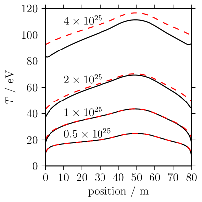
Figure 4: Steady state profiles for 1d SOL simulations using sheath boundary (black) conditions original boundary conditions (red) for several different heat-source amplitudes (in eV/m³/s). Number of moments used is $40\times 4$

In the limit of short collision length, the non-local model asymptotes to local, collisional (Braginskii) fluid closures. In this case the influence of the boundary conditions does not propagate into the domain and it suffices to have the correct fluid velocity and heat-flux at the sheath. Thus when the electron temperature is low enough the sheath boundary conditions described here give the same results as the old ones (used in [2], which impose the correct heat-flux but do not otherwise enforce sheath boundary conditions on the non-local model). However, as the temperature (and hence the collision length) increases it becomes important to use fully correct boundary conditions, as we see in Figure (4) where the temperature profiles in steady-state in a one-dimensional SOL model (see [2] for details) are shown. The only parameter changed is the amplitude of the heat source for the electrons which is used to vary the electron temperature. For low temperatures (up to $\sim$50eV here, corresponding to a collision length of $\sim$4m) both methods give the same results, but at higher temperatures ($\sim$100eV corresponding to a collision length of $\sim$14m) we can see that the details of the boundary conditions have a significant effect on the results.

5 Conclusions

A scheme to give kinetic sheath boundary conditions for non-local parallel closures has been derived and implemented in BOUT++, allowing kinetic effects to be consistently included in fluid models of the SOL. This opens up a much wider parameter space to investigate the behaviour of the SOL plasma through three-dimensional fluid simulations, as these can now be extended to low collisionality.

The change in moment basis also gives an $\mathcal{O}(10)$ speed-up in the evaluation of the closures for typical parameters, making three-dimensional simulations using the non-local code much more readily practicable.

Future work will investigate the extension of the boundary conditions to include the effects of secondary electron emission and begin to apply these non-local closures to three-dimensional SOL simulations, initially focusing on filament dynamics.

References

- [1] B.D. Dudson, X.Q. Xu, M.V. Umansky, H.R. Wilson, and P.B. Snyder. Plasma Physics and Controlled Fusion, 53(5):054005, 2011.
- [2] J.T. Omotani and B.D. Dudson. PPCF, 55(5):055009, 2013.
- [3] J.Y. Ji, E.D. Held, and C.R. Sovinec. Phys. Plasmas, 16(2):022312, 2009.
- [4] J.Y. Ji and E.D. Held. Physics of Plasmas, 13(10):102103, 2006.
- [5] G.W. Hammett and F.W. Perkins. Phys. Rev. Lett., 64:3019–3022, Jun 1990.
- [6] J.T. Omotani, N.R. Walkden, B.D. Dudson, and G. Fishpool. EPS Conference on Plasma Physics, http://ocs.ciemat.es/EPS2013PAP/pdf/P1.108.pdf, 2013.