On The Scalability of P2P Swarming Systems

Abstract

One of the fundamental problems in the realm of peer-to-peer systems is that of determining their service capacities. In this paper we focus on P2P scalability issues and propose models to compute the achievable throughput under distinct policies for selecting both peers and blocks. From these models, we obtain novel insights on the behavior of P2P swarming systems that motivate new mechanisms for publishers and peers to improve the overall performance. In particular, we obtain operational regions for swarm system. In addition, we show that system capacity significantly increases if publishers adopt the most deprived peer selection and peers reduce their service rates when they have all the file blocks but one.

1 Introduction

Peer-to-peer (P2P) swarming systems have been tremendously successful in disseminating content in the Internet and major companies have adopted this architecture. For instance, Blizzard entertainment distributes large files via the Blizzard downloader, which is based on the BitTorrent Opensource. Ubuntu Linux is also available to download via BitTorrent and the Amazon Simple Storage Service (Amazon S3) supports the BitTorrent protocol for distributing files. In addition, recent proposals suggest the use of P2P for distributing large files in content oriented networks [19] paving the way towards a Network Swarm Architecture.

P2P architectures have been studied for over a decade and numerous models have been proposed to address the performance of the approach. Examples include models to determine the impact of incentive mechanisms and download/upload rates on performance [12, 6], fairness [29] and availability [10]. In addition, several works have focused on block distribution and peer selection strategies [23], and proposed improvements to the standard BitTorrent protocol [41].

Despite numerous papers in the area, scalability issues have only recently been addressed. A system scales if its throughput, i.e., the rate at which users complete their downloads, increases linearly with increasing user population. P2P systems have been thought to be scalable since each new user joining the system brings additional resources to it. Consequently, the total capacity available is expected to increase in proportion to the newly incorporated resources and, accordingly, system throughput should increase linearly and unboundedly with population size. However, intrinsic limitations of the P2P architecture to scale in this manner have been observed. Hajek and Zhou [17] showed that, when peers in a swarm and publisher adopt a random peer/random useful block policy, the system is unstable, that is, swarm population grows without bound if peer arrival rate $\lambda$ exceeds the server capacity ($U$) dedicated to that swarm. Briefly, this instability occurs because, when two peers meet, they may not have useful data to share. Understanding the stability region of peer-to-peer swarming systems has recently gained attention [25, 47, 17, 26], and unstable scenarios have been observed in practice [29, 28].

In a peer-to-peer swarming system, each peer makes two decisions before transmitting a block: $(a)$ what block to transmit and $(b)$ to whom to transmit it. Although the former decision has received some attention in previous works (for instance, it has been shown that rarest-first block selection and random useful block selection yield the same stability region [17]), the implication of the peer selection strategy on throughput has not been thoroughly studied (notable exceptions being [25, 26]). Previous works have assumed peers choose their neighbors using random peer selection [32, 47, 17].

In this work we evaluate the impact of different system parameters and system strategies on attainable throughput. Our key contributions are:

System throughput upper-bound. First, we derive an upper bound on the throughput achieved when the publisher adopts most deprived peer selection and rarest-first block selection, while peers adopt random peer selection and random useful block selection. The bound is significantly larger than the maximum attainable throughput observed in the scenarios studied in [17], where both peers and publishers adopt random peer and random useful block selection. This means that system performance can substantially increase if the server adopts a simple policy that gives priority to those peers that possess the smallest number of blocks in the swarm.

Stability region characterization. We identified two regions in which the P2P systems can operate. Such regions are characterized by two thresholds, referred to as the critical and saturation thresholds, denoted by $\lambda_{C}$ and $\lambda_{S}$, respectively, where $\lambda_{C}<\lambda_{S}$. The corresponding throughputs are given by $\Gamma_{C}$ and $\Gamma_{S}$, respectively, where $\Gamma_{C}=\lambda_{C}$ and $\Gamma_{S}\leq\lambda_{S}$. In the first region, $\lambda<\lambda_{C}$, the system is stable, i.e., download times are finite. In the second region, $\lambda_{C}<\lambda<\lambda_{S}$, the system is unstable, i.e., delays are infinite but throughput grows as arrival rate increases. In the third region, $\lambda>\lambda_{S}$, the system is unstable and throughput equals $\Gamma_{S}$.

Benefits of upload throttling, protection of newcomers and admission control. Our models suggest a new very simple and incentive-compatible policy adopted by peers, wherein peers reduce their service capacity when they possess all blocks but one (see Section 3). By employing this upload throttling policy, which requires only changes to the protocol implemented by peers, the system can accommodate more users while remaining stable, specially when near saturation. In addition, we also investigate policies that involve changes to peers and trackers, wherein trackers protect newcomers to be preferably served by the publisher (see Section 5). Numerical results indicate that such policies, in addition to admission control, can also result in significant performance gains.

Paper structure

The remainder of this paper is organized as follows. In Section 2 we set the background, discuss the scalability problem and compare several peer and server policies. In Section 3 we describe the models used to obtain the results we present. Analytical and numerical results obtained from the models are discussed in Sections 4 and 5, respectively. We show how system throughput scales with swarm population size and study the performance gains of the policies we propose. Related work is presented in Section 6, Section 7 summarizes our assumptions and model limitations, and Section 8 concludes our work.

2 Scalability of Peer-to-Peer Systems

In a P2P system, every new peer entering a swarm brings additional resources (transmission capacity and storage) to it since it acts both as a client and as a content provider. Therefore it is natural to expect the overall system throughput to increase as the number of peers increases. However, the throughput growth is not unbounded. Figure 1, obtained from one of the models we developed (Section 3.2) illustrates this well. Let $\lambda$ denote the arrival rate of peers to a swarm.

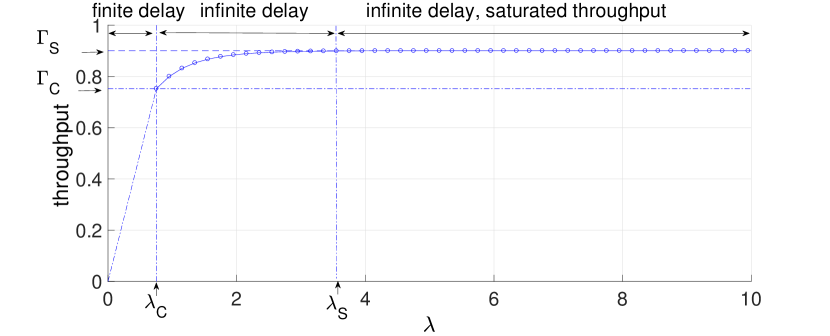
Figure 1: System throughput (3 blocks, most deprived peer, rarest first chunk, $\mu=0.5$, $U=0.3$)

Illustrative example

To appreciate the nature of our results through a simple example, Figure 1 shows how the throughput varies as a function of the arrival rate, for a given peer and server capacities allocated to the swarm. (The notation is defined in Table 2.) Figure 1 shows that throughput grows linearly in $\lambda$ until $\lambda$ reaches a threshold ($\lambda_{C}$). Download delays are finite in the region $\lambda<\lambda_{C}$ and infinite when $\lambda>\lambda_{C}$. When $\lambda=\lambda_{C}$, throughput equals arrival rate, $\Gamma_{C}=\lambda_{C}$. When $\lambda\geq\lambda_{C}$, throughput increases until $\lambda$ reaches a threshold $\lambda_{S}$, meaning that it is possible to achieve higher throughput at the cost of infinite delays. When throughput reaches $\Gamma_{S}$ the system is fully saturated and throughput no longer increases in $\lambda$. Briefly, although available resources increase as the number of peers increases (increasing $\lambda$), they are not fully utilized. For instance, this occurs when a peer has no block different from those its neighboring peers possess; thus, its service capacity is wasted.

Two fundamental operating regimes

There are two operating regimes observed in the P2P systems of interest to us. One is a stable operating regime where all peers that arrive acquire the content in a finite amount of time. Associated with this regime is a threshold $\lambda_{C}$ such that the system is stable provided the peer arrival rate $\lambda$ satisfies $\lambda<\lambda_{C}$. Then, there is a second regime where the maximum achievable throughput, $\Gamma_{S}$, referred to as the saturation throughput, can be larger than $\Gamma_{C}$ (see Figure 1). To leverage the possibility of achieving a throughput larger than $\Gamma_{C}$, our study suggests that it is interesting to implement admission control, so as to achieve a throughput larger than $\Gamma_{C}$ without incurring infinite download delays.

In light of the two operating regimes discussed above, we briefly provide further insight on the throughput curve of Figure 1. Consider a P2P system in which peers leave as soon as they complete their downloads. The file downloaded by a particular swarm is divided into $K$ equal size blocks. Recall that $U$ is the server capacity allocated to the swarm in blocks per time unit. Let $\mu$ be the service capacity of each peer, also measured in blocks per time unit. When peer arrival rates are large relative to $U$ the system will reach, with high probability, a state in which all peers have all but one of the blocks (say, block $\mathcal{B}$). In this scenario, only the server has block $\mathcal{B}$ and as soon as a peer obtains the missing block $\mathcal{B}$ from the server it leaves the system without helping to serve block $\mathcal{B}$ to others. On the other hand, new peers that arrive are quickly served by their peers and are able to obtain all blocks but $\mathcal{B}$. As a consequence, the system behaves approximately like a client server system: peers depart at rate $U$ since they do not cooperate to obtain the missing block. In addition, although available resources grow with the swarm size, these resources are not fully utilized.

We propose a queueing model in Section 3 to estimate the throughput taking into account that, when the system is saturated, with high probability most peers in the system eventually obtain all but the rarest block. We also show that the throughput depends on service policies adopted by the server and peers.

Neighbor and block selection policies

In a P2P system, the publisher needs to decide what block to transmit next and to which peer. Likewise, a peer has to decide what peer to contact and which block to request. In the literature, it has been assumed that peers go through random encounters and that peers are paired uniformly at random [17, 33, 44]. Nonetheless, if the publisher can strategically select peers to serve, then it is possible to improve the overall system capacity. Before introducing our models we first describe the policies that we consider.

Random peer selection

Throughout this paper, except otherwise noted we assume that peers select a neighbor uniformly at random at every transmission opportunity to exchange blocks. Such policy is referred to as random peer selection policy.

Random useful peer selection

We also consider the case where trackers dynamically inform each peer $P$ in the set of peers in the swarm of those that are in need of blocks owned by $P$. In this case, peers can select their neighbors uniformly at random among those that need the blocks they possess. We refer to this neighbor selection policy as random useful peer selection.

Random useful block selection

After choosing a neighbor, each peer selects one of its blocks for transmission to the neighbor. If the block is selected uniformly at random, the policy is referred to as random useful block selection.

Rarest first block selection

If peers have access to a list of the number of replicas of each block, they can build a rarest-block set containing the indices of the blocks with the least number of copies in the swarm [20]. This set can then be used by peers to select which block to transmit. This policy is referred to as rarest first block selection.

Most deprived peer selection by publishers

The publisher can select its peers and blocks in the same way as the peers. In addition, the publisher can also select its peers using the most deprived policy. Under this policy, the publisher prioritizes sending blocks to peers that own the least amount of blocks among those in the swarm. If the arrival rate of peers is large (or the swarm size is large) these peers are likely to be content-less peers, also referred to as newcomers. Table 1 summarizes these policies.

peers	publisher
random peer/random useful block (RP/RUB)	random peer/random useful block (RP/RUB)
random peer/rarest first block (RP/RFB)	random peer/rarest first block (RP/RFB)
random useful peer/random useful block (RUP/RUB)	most deprived peer/random useful block (MDP/RUB)
random peer/random useful block (RP/RUB)	most deprived peer/rarest first block (MDP/RFB)

Table 1: Neighbor and block selection policies

3 Models

In this section we present models of the P2P systems utilizing policies presented in the previous section. The key goal of the models is to estimate $\lambda_{C}$ and $\lambda_{S}$, for different server and peer policies.

Using our models we show how throughput depends on different system parameters. Random peer and block selection by peers and publisher have been studied in [17, 47]. These works show that the system is stable if and only if $\lambda<U$. The proposed models allow us to study simple modifications to the peer and block selection policies. For instance, in Section 4 we show that adoption of the most deprived peer selection policy by the publisher can increase throughput. In addition, in Section 5 we show that if peers reduce their service capacity, maximum achievable throughput can be further increased. Table 2 summarizes notation used in this paper.

Variable	Description
System parameters
$\lambda$	peer arrival rate
$U$	the server capacity allocated to a swarm
$K$	total number of blocks
$\tilde{K}$	number of blocks individually accounted by the truncated model
$\mu$	peer service capacity
$\mu^{\prime}$	reduced peer service capacity
$N$	number of peers in the swarm
	(when considering the queuing model, we assume an infinite one-club, so $N=\infty$;
	in Section 4.4, in contrast, we consider a population of fixed finite size $N$)
Throughput-related variables
$\Gamma$	total rate at which peers leave the system (system throughput)
$\lambda_{C}$	critical throughput (when $\lambda<\lambda_{C}$, we have finite delays and a finite population of newcomers)
$\lambda_{S}$	saturation throughput (when $\lambda_{C}<\lambda<\lambda_{S}$ the throughput can still be increased,
	whereas for $\lambda>\lambda_{S}$ we have a saturated system with an infinite population of newcomers)
Queuing model variables
$p$	fraction of blocks served by the publisher that is transmitted to newcomers
	(under MDP/RFB, probability that publisher serves rarest block to newcomer)
$F_{i}$	$i$-th queue containing non-gifted peers that have $i$ blocks
$G_{j}$	$j$-th queue containing gifted peers that have $j$ blocks
$n_{i}$	random variable denoting the number of non-gifted peers that have $i$ blocks
$m_{j}$	random variable denoting the number of gifted peers that have $j$ blocks
	(those peers have the rarest block and additional $(j-1)$ blocks)
$\tilde{m}_{\tilde{K}-1}$	random variable denoting the number of gifted peers that have $\tilde{K}-1$ or more blocks
Queuing model rates
$\gamma_{r}(i)$	rate at which non-gifted peers that have $i$ blocks receive the rarest block
$\gamma_{p}(i)$	rate at which non-gifted peers that have $i$ blocks receive a popular block
$\Psi$	rate at which the gifted peers serve the rarest block to the one-club members

Table 2: Table of notation

3.1 Overview of Peers and Publisher Dynamics

We first consider a publisher policy that gives priority to peers with the smallest number of blocks and serves the rarest block to the chosen peers. That is, the server adopts the MDP/RFB policy (Table 1). In addition, peers adopt the RP/RUB policy, wherein upon a random peer contact, a block is randomly chosen to be downloaded from among those blocks that the recipient peer does not have. We also assume that a peer reduces its service capacity whenever it obtains $K-1$ blocks, changing its service capacity from $\mu$ to $\mu^{\prime}$ where $\mu^{\prime}<\mu$. The motivation for this rate reduction will be clarified below when we show that it significantly increases the system throughput. We refer to Figure 2 to describe the model.

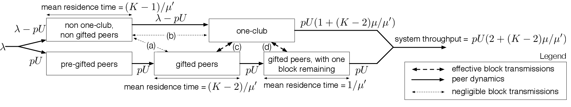
Figure 2: Flow dynamics

In Figure 2 we identify five boxes each representing a set of peers with a given collection of blocks from the downloaded file. Solid (resp., dotted) arrows correspond to peer dynamics (resp., block transmissions). We assume that the peer arrival rate $\lambda$ is sufficiently large, $\lambda>\lambda_{S}>U$, as in Figure 1. In this regime, the system enters a state where an infinite number of peers have all but one of the blocks of the file. These peers are said to belong to the one-club set [17] (see Figure 2).

Since the publisher adopts most deprived peer selection and $U<\lambda$, a fraction $pU/\lambda$ of peers receive a block from the publisher after arriving to the system. Note that: $(a)$ newcomers are content-less, so they are served with higher priority by the publisher and; $(b)$ since $\lambda$ is much larger than $U$, the publisher finds a newcomer with high probability as soon as it is ready to serve a new peer. Parameter $p$ denotes the fraction of blocks served by the publisher to newcomers. It captures the fact that newcomers may not receive all of the publisher capacity available to the swarm. Peers that obtain the rarest block are called gifted peers. The three boxes in the bottom row of Figure 2 represent peers in the process of obtaining the rarest block and those peers that already received it.

Remark: $p=1$ corresponds to the publisher serving the rarest block to a newly arrived peer, whenever the publisher is available upon the arrival under consideration. For this to occur, it may be necessary to postpone the immediate advertisement of newcomers to other peers, i.e., newcomers may be known for some initial time only to the tracker. Otherwise, the server and other peers compete for service. A newly arrived peer may obtain a popular block from other peers, before obtaining the rarest block from the server, even when the server is idle upon arrival. As a result, the competition between server and peers favors $p<1$, where $p$ depends on $U$ and $\mu$. We will return to this issue in Section 5.

Peers adopt random peer and random useful block selection policies. We say a block is popular whenever it is not the rarest block. Note that as the one-club is assumed to be large, the download of the vast majority of the popular blocks involves peer encounters that occur uniformly at random between peers not in the one-club with those in the one-club (arrows $(b),(c)$ and $(d)$ in Figure 2). Since the gifted set is relatively small, roughly all popular blocks are served by the one-club population, and a typical peer takes on average $1/\mu^{\prime}$ to download each popular block. Transmissions of popular blocks not involving a member of the one club, such as those represented by arrow $(a)$ in Figure 2, can be neglected. Note also that as peers select their neighbors uniformly at random, a significant number of peer encounters occurs between members of the one-club amongst themselves. Such encounters produce no exchange of blocks.

It follows from Little’s result that the expected number of peers in each of the boxes shown in Figure 2 is given by the arrival rate to the box multiplied by the corresponding average residence time. In particular, the expected number of gifted peers (resp., gifted peers with one remaining block to download) is $pU(K-2)/\mu^{\prime}$ (resp., $pU/\mu^{\prime}$). Each of these peers serves the one club at rate $\mu$ (resp., $\mu^{\prime}$). Therefore, the departure rate from the one-club is $pU(K-2)\mu/\mu^{\prime}+pU$ (due to arrows $(c)$ and $(d)$ in Figure 2).

Let $\Gamma$ be the system throughput. Then, the above arguments imply that

$$\Gamma=\left(\frac{(K-2)\mu}{\mu^{\prime}}+2\right)pU$$ (1)

We will revisit the result above in Section 4.3, in light of the queueing network model presented in the next section.

3.2 Queueing Network Model

Next, we introduce a queueing network model that captures the throughput achieved by a number of different peer-to-peer swarming policies. The model is motivated by the flow dynamics shown in Figure 2. Figure 3 illustrates the proposed model accounting for a file with $K=3$ blocks (the extension to $K\geq 4$ blocks is straightforward). A fundamental assumption is that there is an infinite number of peers belonging to the one-club.

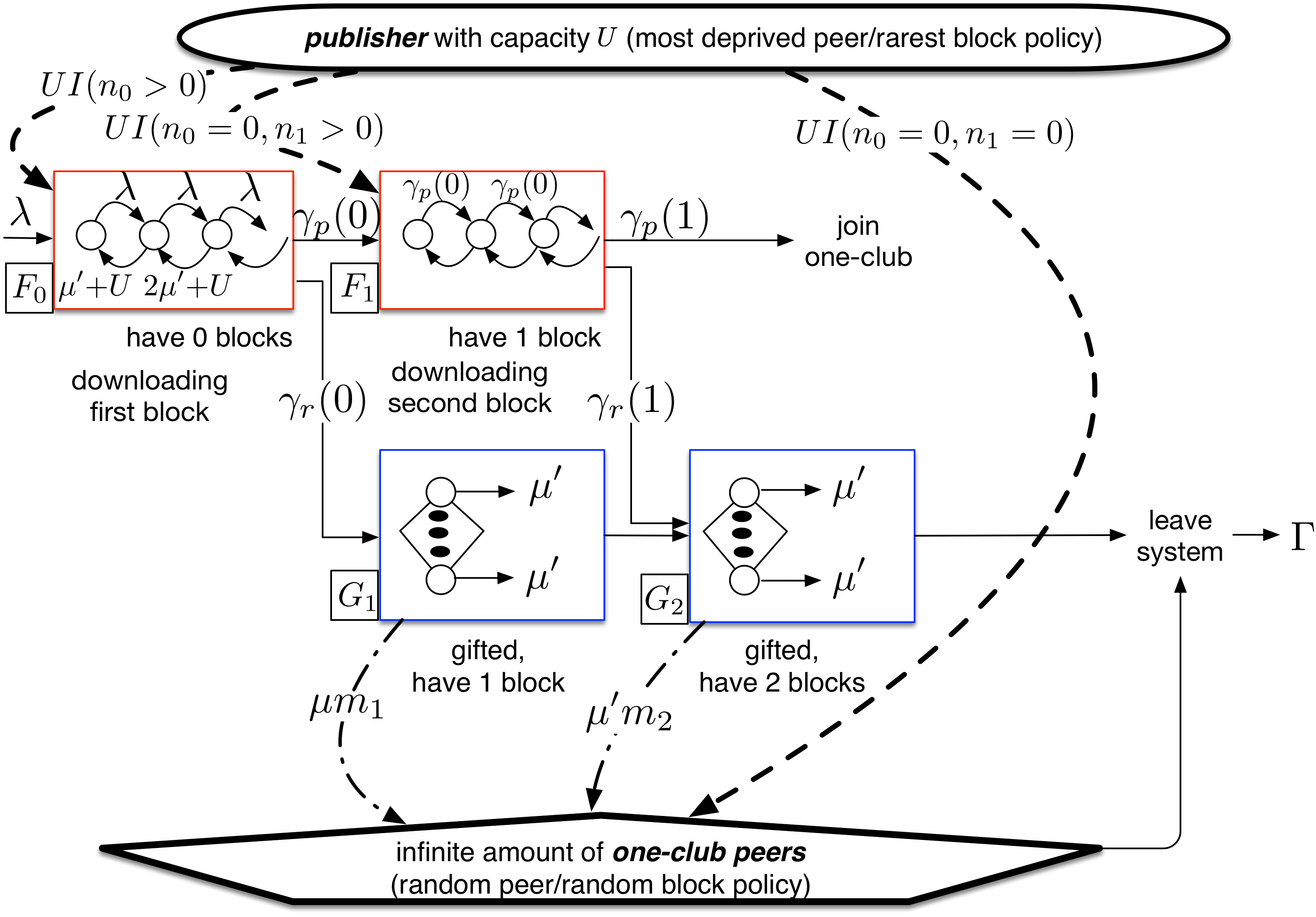
Figure 3: Queueing network model ($K=3$).

Referring to Figure 3, the queues in the top characterize peers that do not have the rarest block. These queues, denoted by $F_{0},\ldots,F_{K-2}$, can be served both by the publisher and other peers. Each of theses queues is modeled as a birth-death process with constant arrival rate and state dependent service capacity as explained below. The first queue (leftmost queue in Figure 3, queue $F_{0}$) represents newcomers. Peers in this queue have no blocks. The remaining queues in the top row represent peers that have already obtained $1,\ldots,K-2$ popular blocks, and are waiting to complete the download of an additional block.

The bottom queues, denoted by $G_{1},\ldots,G_{K-1}$, represent gifted peers. The leftmost queue in the bottom row, $G_{1}$, represents all peers that downloaded only the rarest block. The other queues at the bottom represents peers that possess the rarest block along with $\ell$ popular blocks, $\ell=1,\ldots,K-2$ (queues $G_{2},\ldots,G_{K-1}$, respectively).

Newcomers arrive with rate $\lambda$ and join $F_{0}$. Since these peers have no blocks they can be served either by the publisher (that preferentially serves peers with the least number of blocks) or by other peers. Because the one-club is large by assumption and encounters occur at random, the set of all one-club members serves a block to a tagged newcomer at rate $\mu^{\prime}$.

Let random variables $n_{i}$ and $m_{j}$ denote the number of peers at queues $F_{i}$ and $G_{j}$, respectively, for $i=0,\ldots,K-2$ and $j=1,\ldots,K-1$. In particular, $n_{0}$ denotes the number of newcomers. Let $\gamma_{r}(i)$ and $\gamma_{p}(i)$ denote the rate at which non-gifted peers that have $i$ blocks receive the rarest block and a popular block, respectively. From the above arguments, the rate at which newcomers receive the rarest block is

$$\gamma_{r}(0)=U(1-\pi_{0}(0)),$$ (2)

where $\pi_{0}(0)=\mathbb{P}(n_{0}=0)$ is the probability that the newcomer queue is empty. Note that the rarest block can only be supplied by the publisher, due to the assumption that the one-club is large and the random peer selection policy adopted by the peers. Likewise, let $\gamma_{p}(0)$ denote the rate at which newcomers obtain a popular block. Then,

$$\gamma_{p}(0)=\mathbb{E}[n_{0}]\mu^{\prime},$$ (3)

where $\mathbb{E}[n_{0}]$ is the expected number of newcomers.

If a newcomer gets the rarest block (resp., a popular block) from the publisher (resp., from the one-club), it transitions to queue $G_{1}$ (resp., $F_{1}$). Since peers in $F_{1}$ have only one popular block, they are eligible to be served by the publisher, provided that queue $F_{0}$ is empty (most deprived policy). Similar to those peers in $F_{0}$, those in $F_{1}$ can also be served by the one-club.

Gifted peers in $G_{1}$ can only be served by one-club members, since the publisher gives preference to those peers that do not have the rarest block. Recall that $m_{j}$ is the number of gifted peers that have the rarest block in addition to $j-1$ blocks. Queue $G_{j}$ is then modeled as an M/M/$\infty$ queue with aggregate departure rate $\mu^{\prime}m_{j}$, $j=1,\ldots,K-1$. Once peers in $G_{j}$ obtain a popular block, they move to queue $G_{j+1}$ to get an additional (popular) block, for $j=1,\ldots,K-2$. Finally, after downloading the rarest block and $K-2$ popular blocks peers move to queue $G_{K-1}$, which models the peers with $K-1$ blocks, one of them being the rarest. After obtaining an additional block, they leave the system.

The average number of customers at queue $G_{j}$, $j=1,\ldots,K-1$, is given by

$$\mathbb{E}[m_{j}] =\sum_{l=0}^{j-1}\gamma_{r}(l)/\mu^{\prime},\quad j=1,2,\ldots,K-1$$ (4)

as queues $G_{j}$, $j=1,\ldots,K-1$, are M/M/$\infty$ queues with arrival rate $\sum_{l=0}^{j-1}\gamma_{r}(l)$ and mean residence time $1/\mu^{\prime}$ (see Figure 3).

If a peer in $F_{j-1}$ gets a block from the publisher, it moves to queue $G_{j}$. Otherwise, it moves to $F_{j}$, for $j=1,\ldots,K-2$.

Publisher service rate approximation

We should note that the service capacity of queue $F_{i}$ ($i=1,2,\ldots,K-2$) depends on the states of queues $F_{0},\ldots,F_{i-1}$. When queue $F_{i}$ is in state $s$, i.e., when there are $s$ customers at that queue, its service capacity is given by $s\mu^{\prime}+UI[n_{0}=0,\ldots,n_{i-1}=0]$, where $I[\mathcal{E}]=1$ if predicate $\mathcal{E}$ is true and 0 otherwise. As an approximation, we break this dependency by using the independent stationary value $\mathbb{P}(n_{i}=0)$ of each queue $F_{l}$, $l<i$. Therefore, the aggregate rate at which peers in $F_{i}$ are served is approximated as $\mathbb{E}[n_{i}]\mu^{\prime}+U\prod_{l=0}^{i-1}\pi_{0}(l)$. From this, we obtain the rate at which peers in queue $F_{i}$ move to $G_{i+1}$:

$$\gamma_{r}(i)=U\left({\prod_{l=0}^{i-1}\pi_{0}(l)}\right)(1-\pi_{0}(i)),$$ (5)

where the product in parentheses is defined as $1$ when $i=0$. The rate at which peers in $F_{i}$ move to $F_{i+1}$ is:

$$\gamma_{p}(i)=\mathbb{E}[n_{i}]\mu^{\prime}.$$ (6)

Service rate at which one-club is served by gifted

Once the arrival rate at each queue is obtained we compute the rate at which the one-club is served. We observe that peers in queues $G_{1},G_{2},\ldots,G_{K-1}$ possess the rarest block and, therefore, they can serve peers in the one-club. In particular, each tagged peer in $G_{1},G_{2},\ldots,G_{K-2}$ serves the one-club at rate $\mu$. Peers in $G_{K-1}$ serve the one club at rate $\mu^{\prime}$. (Refer to the dashed lines in Figure 3.) Let $\Psi$ be the rate at which the gifted peers serve the rarest block to the one-club members. Then,

$$\Psi = \sum_{j=1}^{K-2}\mu\mathbb{E}[m_{j}]+\mu^{\prime}\mathbb{E}[{m_{K-1}}],$$ (7)

$$= \sum_{j=1}^{K-2}\frac{\mu}{\mu^{\prime}}\sum_{l=0}^{j-1}\gamma_{r}(l)+\sum_{j=0}^{K-2}\gamma_{r}(j),$$ (8)

$$= \frac{\mu}{\mu^{\prime}}\sum_{j=0}^{K-3}(K-2-j)\gamma_{r}(j)+\sum_{j=0}^{K-2}\gamma_{r}(j),$$ (9)

$$= \frac{\mu}{\mu^{\prime}}\sum_{j=0}^{K-2}\left({(K-2-j)+\frac{\mu^{\prime}}{\mu}}\right)\gamma_{r}(j)$$ (10)

where $\gamma_{r}(j)$ is given by (5), and (8) follows by replacing (4) into (7).

System throughput

Let $\Gamma$ be the total rate at which peers leave the system (i.e., the system throughput). Then,

$$\Gamma =\sum_{i=0}^{K-2}\gamma_{r}(i)+\Psi+U\prod_{i=0}^{K-2}\pi_{0}(i).$$ (11)

The first term in the summation in (11) corresponds to the departure rate of the gifted peers, whereas the second and third terms correspond to the rates at which the one-club is served by gifted peers and by the publisher, respectively.

3.3 Model Truncation

To find the critical throughput $\Gamma_{C}$ using the model proposed in the previous section requires the solution of a fixed-point problem encompassing $2(K-1)$ equations (see Section C.2). To reduce the computational complexity when $K$ grows large, in what follows we consider an approach to truncate the model. The proposed truncated model captures the evolution of peers while they download their first few blocks before either entering the one-club or getting the rarest block and then downloading the remaining blocks. Model accuracy depends on the number of first few blocks considered. The accuracy increases with the number of blocks considered, at the cost of increased computational complexity to solve the model.

Let $\tilde{K}$ denote the number of stages taken into account when tracking the download of gifted peers. The first stage (stage zero) corresponds to newcomers that have zero blocks, the $i$-th stage corresponds to peers that downloaded $i$ blocks and are downloading their $(i+1)$-th block, $i=1,\ldots,\tilde{K}-2$, and the last stage corresponds to the download of the last $K-\tilde{K}+1$ blocks. Non-gifted peers start from the same first stage, and evolve through additional $\tilde{K}-2$ stages before entering the one-club. In general, we use symbols with tilda to denote quantities related to the truncated model.

If $K=\tilde{K}$ the truncated model described below is equivalent to the non-truncated model. The truncated model comprises $2(\tilde{K}-1)$ queues. In the remainder of this paper, when $K\geq 4$ we consider an instance of the model which consists of six queues, i.e., $\tilde{K}=4$, and is illustrated in Figure 4. In our experiments this was sufficient to achieve accurate results.

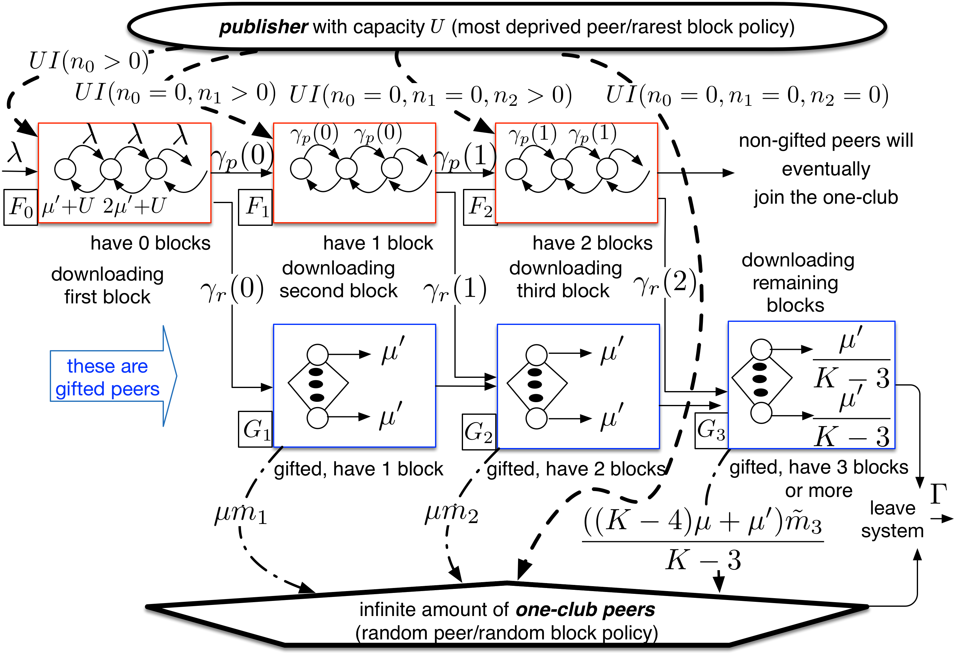
Figure 4: Truncated queueing network model ($\tilde{K}=4$ and $K\geq\tilde{K}$).

Let $F_{i}$ be the $i$-th queue containing non-gifted peers, $i=0,1,2,\ldots,\tilde{K}-2$ and let $G_{j}$ be the $j$-th queue containing gifted peers, $j=1,2,3,\ldots,\tilde{K}-1$. Recall that $m_{j}$ denotes the number of gifted peers that have exactly $k$ blocks. In the truncated model, we denote by $\tilde{m}_{j}$ the number of gifted peers in queue $G_{j}$, $\tilde{m}_{j}=m_{j}$, $j=1,\ldots,\tilde{K}-2$, and further let $\tilde{m}_{\tilde{K}-1}$ denote the number of gifted peers that have $\tilde{K}-1$ or more blocks. The truncated model differs from the model presented in the previous section in two ways described below.

$(a)$ Non-gifted peers with more than $\tilde{K}-2$ blocks are not explicitly taken into account. We assume that the probability that non-gifted peers with more than $\tilde{K}-2$ popular blocks obtain the rarest block from the publisher is negligible. This is true since the publisher gives priority to peers with the least number of blocks. Let $K\geq 4$. If a peer reaches $F_{\tilde{K}-2}$ and then obtains one popular block, it further downloads additional $K-\tilde{K}$ popular blocks and eventually joins the one-club. Non-gifted peers with more than $\tilde{K}-2$ popular blocks are not explicitly represented in the truncated model. These peers have no effect on the model, since with high probability they eventually join the one-club, which is infinite in size.

$(b)$ Gifted peers with more than $\tilde{K}-2$ blocks are combined into a single class. The rightmost queue at the bottom of Figure 4 represents all peers that have the rarest block along with $\tilde{K}-2$ or more popular blocks. Since $G_{\tilde{K}-1}$ models peers that have $\tilde{K}-1$ or more blocks and because this is an M/M/$\infty$ queue, the expected number of peers that have the rarest block plus $\tilde{K}-2,\ldots,K-2$ popular blocks are all identical. Recall that $\tilde{m}_{\tilde{K}-1}$ is the number of peers at queue $G_{\tilde{K}-1}$ and

$$\mathbb{E}[\tilde{m}_{\tilde{K}-1}]=\sum_{l=0}^{\tilde{K}-2}\gamma_{r}(l)\frac{K-\tilde{K}+1}{\mu^{\prime}}.$$ (12)

A fraction $1/(K-(\tilde{K}-1))$ of $\tilde{m}_{\tilde{K}-1}$ have $(K-1)$ blocks and serve the one-club at rate $\mu^{\prime}$ and a fraction $(K-\tilde{K})/(K-(\tilde{K}-1))$ have $\tilde{K}-1,\ldots,K-2$ blocks and serve the one-club at rate $\mu$.

Recall that $\Psi$ is the rate at which the gifted peers serve the rarest block to the one-club members. Then, following the same rationale as in (7)-(10),

$$\Psi = \sum_{j=1}^{\tilde{K}-1}\mu\mathbb{E}[m_{j}]+\frac{(K-(\tilde{K}+1))\mu+\mu^{\prime}}{K-\tilde{K}+1}\mathbb{E}[\tilde{m}_{{\tilde{K}}-1}]$$ (13)

$$= \sum_{j=1}^{\tilde{K}-1}\frac{\mu}{\mu^{\prime}}\sum_{l=0}^{j-1}\gamma_{r}(l)+\frac{(K-(\tilde{K}+1))\mu+\mu^{\prime}}{\mu^{\prime}}\sum_{j=0}^{\tilde{K}-1}\gamma_{r}(j)$$ (14)

$$= \frac{\mu}{\mu^{\prime}}\sum_{j=0}^{\tilde{K}-2}(\tilde{K}-1-j)\gamma_{r}(j)+\frac{(K-(\tilde{K}+1))\mu+\mu^{\prime}}{\mu^{\prime}}\sum_{j=0}^{\tilde{K}-1}\gamma_{r}(j)$$ (15)

$$= \frac{\mu}{\mu^{\prime}}\sum_{j=0}^{\tilde{K}-1}\left({(K-2-j)+\frac{\mu^{\prime}}{\mu}}\right)\gamma_{r}(j)$$ (16)

In what follows, we will use the expression of $\Psi$ derived above to assess system throughput.

System throughput

The system throughput under the truncated model follows the same rationale as in (11), and is given by

$${\Gamma}=\sum_{i=0}^{\tilde{K}-1}\gamma_{r}(i)+\Psi+U\prod_{i=0}^{\tilde{K}-1}\pi_{0}(i).$$ (17)

The rationale for the terms in the equation above is presented below (11).

In what follows, we will use (17) to obtain bounds on the system throughput (Section 4), as well as to numerically assess how the throughput varies as a function of different system parameters (Section 5).

3.4 Model Summary

Table 3 summarizes the rates associated with each of the six queues that comprise the proposed model. As shown in the third column of Table 3, all queues have a component of their service capacity that scales with respect to the number of customers in that queue. Such a component captures the self-scaling property of peer-to-peer swarming systems. In addition, queues $F_{j}$, $j=0,1,2,\ldots,\tilde{K}-2$, also have a constant service capacity component, due to the publisher.

As all queues explicitly captured by the model have a self-scaling component, they are by construction stable. Nonetheless, the one-club population is assumed to be infinite in size and remains so if the arrival rate is greater than the system departure rate. For this reason, if $\lambda>\Gamma$ the system is unstable and peers experience infinite delays. Otherwise, the one-club will eventually vanish and peers experience finite delays. These two regimes are further discussed in Section 4.1 (see also Appendix A).

The third column in Table 3 shows the departure rate at each of the possible states at each queue. It accounts for the stochastic nature of the system. The fourth column, in contrast, presents only averages and accounts for the simplifying assumption of independence between queues. In the fourth column, we replace the event denoting that queues $F_{0},\ldots,F_{j-1}$ are empty, $\cap_{l=0}^{j-1}\{n_{l}=0\}$, by the corresponding product of probabilities $\prod_{l=0}^{j-1}\pi_{0}(l)$.

Finally, note that equating the second and fourth columns of Table 3 the values of $\mathbb{E}[n_{j}]$, $\mathbb{E}[m_{j}]$ and $\mathbb{E}[\tilde{m}_{\tilde{K}-1}]$ immediately follow. In particular, from the last two lines we obtain (4) and (12).

queue	arrival rate	departure rate from state $s$	average departure rate
Newcomers queue
$F_{0}$	$\lambda$	$I(s>0)U+s\mu^{\prime}$	$(1-\pi_{0}(0))U+\mathbb{E}[n_{0}]\mu^{\prime}$
Intermediary non-gifted peers queues ($j=1,2,\ldots,\tilde{K}-2$)
$F_{j}$	$\gamma_{p}(j)+(1-\pi_{0}(j))U\prod_{l=0}^{j-1}\pi_{0}(l)$	$I(s>0\textrm{ and }\cap_{l=0}^{j-1}\{n_{l}=0\})U+s\mu^{\prime}$	$(1-\pi_{0}(j))U\prod_{l=0}^{j-1}\pi_{0}(l)+\mathbb{E}[n_{j}]\mu^{\prime}$
Gifted peers queues ($j=1,2,\ldots,\tilde{K}-2$)
$G_{j}$	$\sum_{l=0}^{j-1}\gamma_{r}(l)$	$s\mu^{\prime}$	$\mathbb{E}[m_{j}]\mu^{\prime}$
$G_{\tilde{K}-1}$	$\sum_{l=0}^{\tilde{K}-2}\gamma_{r}(l)$	$s\mu^{\prime}/(K-(\tilde{K}-1))$	$\mathbb{E}[\tilde{m}_{\tilde{K}-1}]\mu^{\prime}/(K-(\tilde{K}-1))$

Table 3: Queueing model summary

4 System Throughput Analysis

The goals of this section are to a) obtain bounds on the system throughput, b) validate the model introduced in the previous section, and c) indicate the potential advantages of admission control. To these aims, we first analyze the model proposed in the previous section subject to increasing arrival rates. While the arrival rate is within the system capacity region ($\lambda\leq\lambda_{C}$), peers experience finite delays (Section 4.2). If the arrival rate is further increased, peers experience infinite delays and $\Gamma\leq\lambda$ (Section 4.3).

Then, to validate the proposed model, in Section 4.4 we introduce a finite state fixed population Markov model, corresponding to a detailed representation of the system. The fixed population model is amenable to exact numerical solution for small populations (e.g., swarms with up to 35 peers are considered in Section 4.4.1). In Section 5 we will use this Markov model to numerically validate the throughput predicted by our proposed model, comparing predicted results against those obtained through exact numerical solution of the fixed population Markov model. In addition, in Section 5 using this model we will observe that throughput initially increases and then decreases, as the population size grows, motivating the benefits of admission control.

4.1 Overview

Table 4 summarizes different system regimes captured by the open queueing model. When $\lambda=0$, the six queues in the open queueing model are empty. The assumption that the system is initialized with a very large one-club implies that the throughput equals the publisher service capacity, $\Gamma=U$, and the one-club will eventually vanish.

As $\lambda$ increases, throughput increases until $\Gamma=\lambda=\lambda_{C}$. Although we are not able to prove the existence and uniqueness of the critical throughput value, we observed a unique value of $\lambda$, $\lambda=\lambda_{C}$, in all the numerical experiments, for which the queueing model yields $\Gamma=\lambda$. The throughput $\Gamma_{C}=\lambda_{C}$ approximates the behavior of the system with a fixed population size, wherein a new arrival occurs immediately after every departure.

Referring back to Figure 1, when $\lambda\leq\lambda_{C}$ the curve shows that system throughput equals its arrival rate. This is because Figure 1 shows throughput due to arrivals of newcomers. Nonetheless, as the proposed model accounts for a large one-club, and the dynamics of the one-club is out of the scope of the model, at steady state we may have $\Gamma>\lambda$. If we also account for the contribution of the initially large one-club towards the throughput, the throughput curve remains above the line $x=y$ up to reaching the point $\lambda=\lambda_{C}$ (see Appendix A).

It follows from the discussion above that when $\lambda\leq\lambda_{C}$, we have $\Gamma\geq\lambda$, which implies that all arrivals are served and additional departures occur from the one-club. As our model predicts that the one-club eventually vanishes in this regime, we refer to it as finite delay regime. In contrast, when $\lambda>\lambda_{C}$, we have $\Gamma\leq\lambda$, implying that some arrivals join the one-club, which in this case grows unboundedly. For this reason, we refer to this regime as infinite delay regime. If the arrival rate is further increased, the system fully saturates and the throughput never surpasses $\Gamma_{S}$. Additional numerical results illustrating the different system regimes are presented in Appendix A.

regime	throughput	description
$\lambda=0$	$U$	all departures occur from the one-club (which eventually vanishes)
$\lambda<\lambda_{C}$	$\geq\lambda$	all arrivals are served and additional
		departures occur from the one-club (which eventually vanishes)
$\lambda=\lambda_{C}$	$\Gamma_{C}=\lambda_{C}$	critical regime, which approximates
		the behavior of the system with a fixed population size
$\lambda_{C}<\lambda<\lambda_{S}$	$\leq\lambda$	saturated system, wherein new arrivals experience infinite delays
		(and one-club grows unboundedly). Note: $\lambda_{S}\geq\Gamma_{S}$
$\lambda\geq\lambda_{S}$	$\Gamma_{S}$	$\Gamma_{S}$ is the maximum throughput achievable by the open system

Table 4: Overview of system regimes as captured by the open queueing model.

Figure 5 complements Table 4 and summarizes the two operating regimes observed in P2P systems of interest to us.

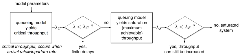
Figure 5: System throughput regions: (a) when $\lambda<\lambda_{C}$, finite delays (model assumes $\infty$ one-club); (b) $\lambda_{C}<\lambda<\lambda_{S}$, infinite delays (model assumes $\infty$ one-club, and a server always busy serving newcomers).

4.2 Critical Throughput $\Gamma_{C}$

Recall that the critical throughput $\Gamma_{C}=\lambda_{C}$ is defined such that for $\lambda\leq\lambda_{C}$ system departure rate equals its arrival rate, i.e., $\Gamma=\lambda$, accounting for throughput due to arrivals of newcomers. We formulate and solve a fixed point problem to obtain $\Gamma_{C}$. The iterative algorithm is described in Appendix B.

To validate the critical throughput obtained using the proposed model, we introduce a detailed fixed size population model in Section 4.4. Under such a closed model, every departure is immediately followed by an arrival, which corresponds to letting the departure rate equal the arrival rate in the open population model. We numerically compare the results obtained using the two models in Section 5.

4.3 Saturation Throughput $\Gamma_{S}$

Next, we use the proposed model to estimate the throughput when the publisher is able to use all its bandwidth on newcomers and is always busy. We derive the saturation throughput using the queueing model, and present two alternative derivations to obtain the same result in Appendix C.

4.3.1 Queueing Network Model

Proposition 4.1

When the server adopts the MDP/RFB policy, peers adopt the RP/RUB policy and all the publisher service capacity is devoted to newcomers, the system throughput is limited by

$$\Gamma_{S}=\left(\frac{(K-2)\mu}{\mu^{\prime}}+2\right)U$$ (18)

Proof: We use the queueing network model to obtain (18). We consider a saturated system, wherein the service capacity of the publisher is devoted to newcomers. Therefore, $\gamma_{r}(0)=U$, and $\gamma_{r}(i)=0$ for $i=1,2,\ldots,K-2$. This means that peers in $F_{1},F_{2},\ldots,F_{K-2}$ will join the one-club. In addition, the arrival rate to queues $G_{1},G_{2},G_{3},\ldots,G_{K-1}$ is $U$, since the server only serves newcomers. Then, (10) reduces to

$$\Psi=\frac{\mu}{\mu^{\prime}}(K-2)U+U$$ (19)

Substituting (19) into (11) yields

$$\Gamma_{S}=\frac{\mu}{\mu^{\prime}}(K-2)U+2U=\left(\frac{\mu}{\mu^{\prime}}(K-2)+2\right)U$$ (20)

Note that $\pi_{0}(0)$ can be made arbitrarily close to zero by increasing the arrival rate $\lambda$. Therefore, for a large enough $\lambda$ all assumptions of the proposition hold, and the result follows. $\Box$

4.3.2 Discussion

• Zhou and Hajek [17] showed that the limiting throughput is $U$ for the random peer/random useful block selection policy. Proposition 4.1 indicates that, if the publisher adopts the most deprived peer and rarest first block policy, the largest peer arrival rate that the system can support is $(((K-2)\mu/\mu^{\prime})+2)U$. That is, with a minor change in the publisher policy, the achievable throughput can be significantly increased.

• The larger the number of blocks the larger is the maximum achievable throughput, which quantifies the advantage of dividing a file into small blocks. However, one cannot reduce the block size towards zero, due to inherent overhead introduced by headers associated with each block. Future works consists of using Proposition 4.1 to cope with the trade-off between decreasing the block size and increasing the overhead of headers and other control data that is transmitted per block.

• The proposition states a counter-intuitive result. If peers reduce their upload rate once they obtain all but one of the blocks, the system throughput increases inversely to $\mu^{\prime}$. Reducing $\mu^{\prime}$ saves peer bandwidth, increases throughput and is incentive-compatible. Note that equation (18) does not impose any limit to $\mu^{\prime}$. If $\mu^{\prime}$ decreases towards zero, at some point the throughput may decrease. In Section 5, we indicate through a few examples that $\mu^{\prime}$ can be made more than one order of magnitude smaller than $\mu$, which is sufficient for large performance gains.

4.4 Evaluating the Throughput Attained by Fixed Size Populations

Next, we develop a detailed Markov model that allows us to obtain throughput as a function of the number of peers in the swarm for different server and peer policies (Table 1). The model implements fundamental characteristics of the policies studied here and is used for validation purposes to support the findings of this work. Due to the size of its state space, solving it numerically is limited to a relatively small number of blocks and moderate population sizes. Nevertheless, the results clearly support our main conclusions. Next, we present an overview of the Markov model. For a detailed description see Appendix D.

We model a fixed size population system (closed system). As such, whenever a peer leaves the swarm, a newcomer immediately arrives. Therefore, it approximates the behavior of swarms whose populations are approximately constant and allows us to study system bottlenecks as population size grows. Although closed and open systems exhibit different behavior (e.g.,  [38]), the closed system provides insights into the stability region of the corresponding open system. In addition, the closed system can be used to assess the asymptotic throughput of real swarms, through controlled experiments [28].

Recall that $N$ is the number of peers in the swarm. A naïve choice of state description consists of tracking the identities of the blocks that each peer possesses. Clearly, this leads to a state space explosion and is intractable even for small peer populations and numbers of blocks. However, the model has symmetries that can be leveraged to lump the state space (see Appendix E). Let $\Omega$ denote the model state space. One such symmetry allows us to characterize each state ${\mbox{\boldmath$\sigma$}}\in\Omega$ as a vector ${\mbox{\boldmath$\sigma$}}=(\sigma_{1},\ldots\sigma_{M})$ where $\sigma_{i}$ is the number of peers with signature $i$ and $M=2^{K}-1$ is the total number of signatures. Other symmetries allow for additional reductions of the state space cardinality of about one order of magnitude. Due to space limitations we briefly discuss such less evident symmetries, using a simple example. Assume the file contains $3$ blocks, namely $\mathcal{B}_{1}$, $\mathcal{B}_{2}$ and $\mathcal{B}_{3}$. Each of these blocks may become the rarest. Suppose that $R$ peers have all blocks except block $\mathcal{B}_{1}$ and $N-R$ peers have only the rarest block. It is not difficult to verify that this state can be lumped with similar states in which the rarest block is $\mathcal{B}_{2}$ or $\mathcal{B}_{3}$. Our Markov model takes into account states that can be lumped before their generation (see Appendix E).

4.4.1 Illustrative Example

Figure 6 plots the throughput obtained from the detailed Markov model for different publisher and peer policies in Table 1. Although not all possible combinations of policies in Table 1 are shown in Fig. 6, the conclusions we obtain from the figure are valid in a broader set of settings. In Figure 6 we let $K=3$, $U=1$ and $\mu=\mu^{\prime}=0.5$.

In what follows, we assume that peers leave the system immediately after completing their downloads. Appendices F.1 and G consider the case where peers remain in the system as seeds after download completion.

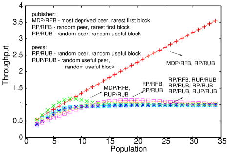
Figure 6: Comparing different policies under the fixed-size population model.

From Figure 6 it is evident that the largest throughput values are obtained when the publisher adopts the MDP/RFB and peers use the RP/RUB policies, for moderate to high swarm population sizes. This is true for a wide range of parameter values. Therefore, we choose to focus our results on this policy in Section 5. The advantages of the MDP/RFB policy adopted by the publisher will be quantified in what follows.

Figure 6 shows, in particular, that the adoption of RP/RUB by peers leads to larger throughputs than RUP/RUB. If peers adopt the random useful peer policy (RUP), one-club members prioritize the service of gifted peers. This, in turn, leads to a reduction of the mean residence time of the latter, and a corresponding system throughput reduction.

Another important feature shown in Figure 6 concerns the maximum throughput achievable in the closed system. Note that the throughput of MDP/RFB, RP/RUB surpasses the threshold $\Gamma_{S}=KU$. This is because the boundary conditions imposed by the closed-system naturally prevent the one-club to grow, which in some settings translates into increased block diversity and a consequent increase in throughput. Such observation is well aligned with cautionary tales discussed in [38], which should be kept under consideration when contrasting open and closed systems. In summary, the closed system is instrumental to validate the critical throughput $\lambda_{C}$, as we will show in the upcoming sections, as well as to motivate the study of admission control, as considered in Section 5. In what follows, we also indicate its applicability to the transient analysis of the system.

4.4.2 Transient Analysis

Next, we provide insight into transient system behavior. To this aim, we consider the fixed population model under the same setup as described in the previous section. We consider a file with size $K=3$ blocks and a population of 15 peers. Assume that initially all peers have no blocks. Peers adopt the RP/RUB policy, whereas the publisher policy is varied according to the experimental goals.

Let the random variable $T$ denote the time it takes until $90$% of the peer population has all blocks except the rarest. Figure 7(a) shows the cumulative distribution function (CDF) of $T$. We see that $\mathbb{P}(T\leq 50)>0.9$ for all the policies considered. For comparison purposes, we note that by $t=50$ we observed in our numerical experiments that an average of approximately $25$ (resp., $50$) peers left the system, when $U=0.5$ (resp., $U=1.0$).

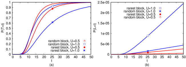
Figure 7: Peers evolving with time in a swarm: distribution of time until $(a)$ all peers enter the one-club and $(b)$ half population leaves the one-club. The publisher selects peers uniformly at random and its block selection policy varies. Peers adopt the random peer/random block policy ($\mu=1.0$).

Once the system reaches the state where most peers have all but the rarest block, it takes considerable time to leave that state. This is shown in Figure 7(b). We assume that at $t=0$ all peers have all blocks but the rarest (except a single peer that has no blocks). Let random variable $L$ denote the time it takes until $50$% of the peers leave the one-club, $i.e.$, until less than 8 peers have all blocks except the rarest. Figure 7(b) shows the CDF of $L$. At $t=50$, the probability that less than 8 peers have all blocks except the rarest is less than $10^{-4}$ for all policies considered.

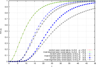
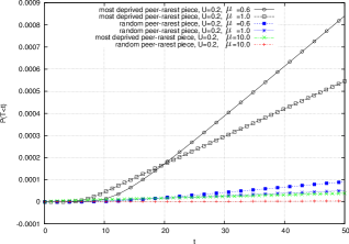
(a) time to enter one-club

(b) time to leave one-club

Figure 8: Transient analysis with most-deprived peer selection.

In Figure 8 we illustrate gains obtained when the publisher adopts the most-deprived peer policy. The larger the difference between $U$ and $\mu$, the more significant are the gains of using the most-deprived peer policy as opposed to the random peer selection. This is expressed both in terms of time to enter a state where 90% of the population is in the one-club starting from an empty system (Figure 8(a)), as well as the time to leave the state where all peers are in the one-club, and reach a state where less than half of the population has all blocks except one (Figure 8(b)).

Using the fixed size population model, we are able to compute transient metrics which would otherwise be very costly to obtain using an open model. The larger state space cardinality of the open model, together with the fact that the system may be unstable under the settings of interest, are two of the challenges that in practice allow the open model to only be solved through simulations. With the fixed size population model, we were able to numerically solve the Markov model and obtain the transient results presented in this section.

5 Numerical Results

In this section we present numerical results obtained with the queueing network model and the detailed Markov model. The results presented in this section complement emulations with real BitTorrent clients present in [28], which showed that the missing piece syndrome can occur in practice, and that the assessment of throughput must account for it. Our goals are to: $(a)$ use the detailed Markov model to validate the queueing network model; $(b)$ show how the throughput varies with different model parameters and $(c)$ motivate the proposed server and peer policies.

5.1 Validating Critical Throughput $\lambda_{C}$

We first use the detailed Markov model to validate the critical throughput $\lambda_{C}$ estimates obtained from the queueing network model. We consider two scenarios, $U\leq\mu$ and $U>\mu$. In what follows, we let $K=3$ and $\mu=\mu^{\prime}$.

In Figures 9(a) and 9(b) we consider scenarios where $U\leq\mu$ and $U>\mu$, respectively. In these figures we present throughput results obtained using three approaches: $(a)$ numerical solution of the detailed Markov model for population sizes varying from 2 to 30 users, using the GTH solution method [16], $(b)$ simulations of the detailed Markov model for population sizes ranging from 2 to 250 users, and $(c)$ asymptotic throughputs computed using the queueing network model. As a sanity check, we verify that the solutions obtained using the GTH method lies within the confidence interval of the simulations. For all values of $U$ and $\mu$, as population increases, throughput increases until it reaches a maximum and then it decreases and tends approximately to $\lambda_{C}$. From the figures we observe that the queueing model presented in Section 3 provides a good estimate of $\lambda_{C}$, the maximum relative error being equal to 10%.

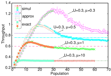
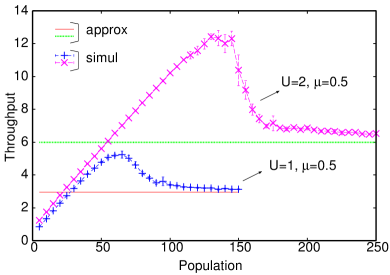
(a) $U\leq\mu$ ($U=0.3$)

(b) $U>\mu$ ($\mu=0.5$)

Figure 9: Validating the queuing network model, $K=3,\mu=\mu^{\prime}$.

5.2 Impact of Varying Service Capacity of the Server

Figure 10 illustrates how throughput varies with $K$ and $U$. These results were obtained from the queueing network model of Section 3, letting $\mu=\mu^{\prime}=1$. The figure shows that the model captures the fact that the throughput is approximately linear in $K$ and $U$, for constant $\mu$. This occurs because the majority of the server transmissions are for newcomers. Each newcomer that is turned into a gifted peer serves, on average, $K-1$ one-club peers before leaving the system. Thus, for each block served by the publisher, roughly $K$ peers leave the system ($K-1$ from one-club plus one gifted). As the server rate is $U$ blocks per time unit, the system throughput grows linearly with $K$ and $U$.

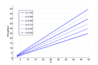
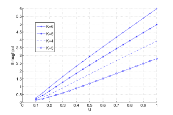
(a) Throughput as a function of $K$

(b) Throughput as a function of $U$

Figure 10: The throughput varies linearly with $U$ and $K$ ($\mu=\mu^{\prime}=1$).

5.3 Uplink Throttling Alleviates the Missing Piece Syndrome

In this section we study system throughput when peers that have collected all blocks but one serve with rate $\mu^{\prime}$, where $\mu^{\prime}<\mu$. The motivation to decrease the upload rate of the one-club peers is to keep the gifted peers in the system longer serving the rarest block. This policy is motivated by the results presented in Section 3.1, which indicate that the throughput can increase if the upload rate of the one-club peers decreases.

Figures 11 and 12 show the increase in throughput when the one-club peers reduce their upload rate from $\mu$ to $\mu^{\prime}$. The figures show that throughput increases as $\mu^{\prime}$ decreases. The proposed policy is very simple and incentive-compatible, allowing peers to increase system performance and save bandwidth.

Figure 12 indicates that the queueing network model predicts an unbounded throughput increase as the upload rate of peers that have all blocks except one decreases, i.e., as $\mu^{\prime}\rightarrow 0$. This is because the queueing network model assumes an infinite one-club. As $\mu^{\prime}$ decreases, gifted peers remain longer in the system, contributing to an increase of the departure rate from the infinite one-club. Nonetheless, if we consider finite populations the throughput decreases as $\mu^{\prime}$ approaches zero. In particular, if $K=2$ and $\mu^{\prime}=0$, the throughput equals $U/2$, since all blocks will be served only by the server (the system degenerates to a client server system).

The results presented so far were obtained using the queueing network model. Figure 12(b), obtained using the detailed Markov model of the closed-system, shows how throughput varies as a function of the population size. We note that the throughput is significantly larger when $\mu^{\prime}<\mu$ for a population greater than 10 users, and as the population grows the throughput gains increase.

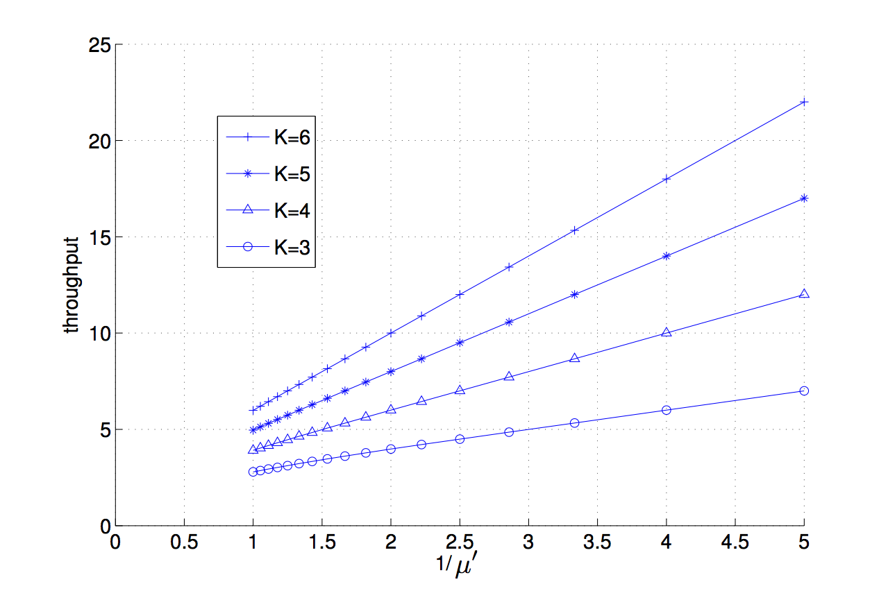
(a)  $\mu=1,U=1$

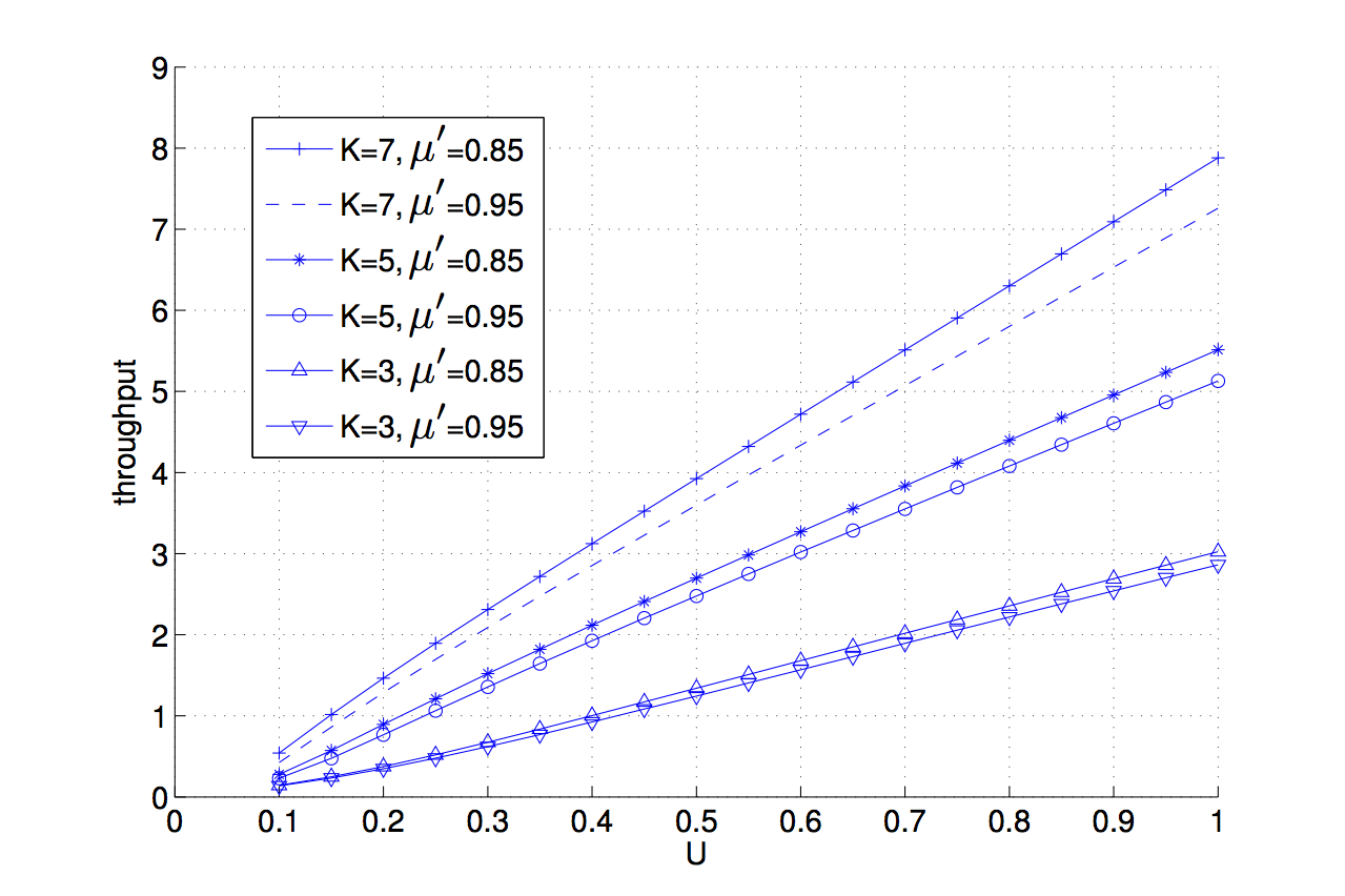
(b)  $\mu=1$

Figure 11: Throughput when policy $\mu^{\prime}<\mu$ is adopted by the one-club peers ($K$ varying between 3 and 7): (a) as $1/\mu^{\prime}$ and (b) $U$ increase, the throughput increases roughly linearly.

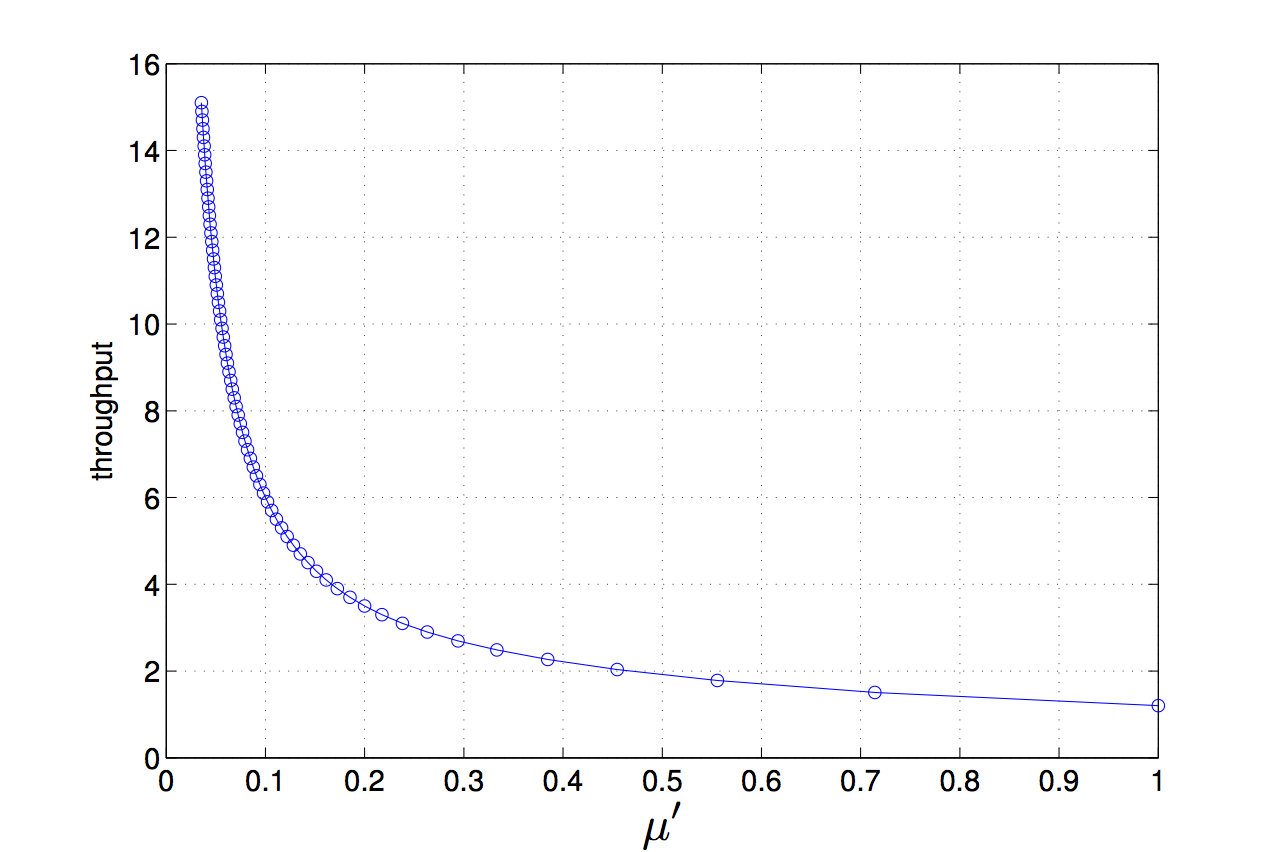
(a)   $K=3,\mu=1,U=0.5$

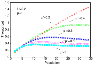
(b)  $K=3,\mu=1,U=0.2$

Figure 12: Throughput when policy $\mu^{\prime}<\mu$ is adopted by the one-club peers ($K=3$).

5.4 Shielding Newcomers Can Further Increase System Throughput

In this section we show scenarios wherein hiding newcomers from other peers can significantly improve system throughput. Under the most-deprived peer policy, the publisher competes against the one-club members to serve newcomers. When $\mu=\mu^{\prime}$, given a large one-club, the publisher serves a newcomer with probability $U/(U+\mu)$. Suppose the server rate $U$ is much smaller than the peer upload rate $\mu$. In this case, newcomers receive, with high probability, the most popular blocks from the one-club members before obtaining the rarest block from the publisher. The idea of shielding a newcomer is to prevent the newcomer from receiving the most popular blocks before it receives the rarest one. This policy is easily implemented by the tracker: it should not announce newcomers to other peers.

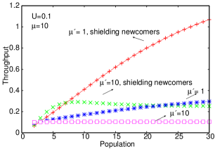
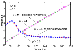
(a) $U<\mu$

(b) $U>\mu$

Figure 13: Throughput when combining the policies of shielding newcomers and setting $\mu^{\prime}<\mu$.

Figure 13, obtained using the detailed Markov model of the fixed-size population system, shows system throughput as a function of population size, when $U<\mu$ and $U>\mu$, for $K=3$. In Figure 13(a), we consider four scenarios: $(i)$ $\mu=\mu^{\prime}=10$, $(ii)$ $\mu=10$ and $\mu^{\prime}=1$, $(iii)$ $\mu=\mu^{\prime}=10$, shielding newcomers and $(iv)$ $\mu=10$ and $\mu^{\prime}=1$, shielding newcomers. In scenario $(i)$, the one-club peers serve newcomers before they receive the rarest block from the server. In this case, system throughput $\Gamma$ converges to the server service capacity, $U$. In the second scenario, one-club peers reduce their upload rate and throughput increases when compared to scenario $(i)$, as expected (see Section 5.3). The third scenario implements the policy of shielding newcomers. The throughput $\lambda_{C}$ is approximately equal to $0.25$. For a small population size, the throughput reaches the value of $\Gamma_{S}$ established in Proposition 4.1. Scenario $(iv)$ combines both policies: the upload rate of one-club peers is reduced and newcomers are shielded. Throughput significantly increases when these policies are used in combination. When the policies are used separately, the throughput is approximately $0.3$ for a population of 30 users. When both policies are used, the throughput exceeds $1.0$.

Figure 13(b) presents the throughput when $U>\mu$. The figure shows that, in this case, the policy of shielding newcomers does not help to improve throughput. When server capacity $U$ is greater than the upload rate of the one-club peers $\mu$, the server transmits the rarest block to newcomers at a higher rate than the rate at which they receive the most popular blocks. It is unnecessary to hide the newcomers from the one-club peers because the former will spontaneously receive the rarest block from the latter before receiving other blocks from the remaining peers. However, throttling the upload capacity for one-club peers continues to be very effective.

5.5 Assessing the Benefits of Admission Control

Next, we present the benefits of admission control. As shown in Figure 9 (fixed-size population model), as population size grows, the throughput initially increases and then decreases. This behavior suggests that it may be beneficial to exert control over the size of the population that participate in the swarm.

Figure 14 confirms the potential benefits of admission control. The curves in Figure 14 were obtained using the model described in Appendix A. We considered an infinite population of peers, joining a system under admission control. In contrast to Section 4.4, we allow the population size to vary over time. We let $\lambda=6$ peers/s, $K=3$, $U\in\{2,0.3\}$ blocks/s and $\mu=\mu^{\prime}=0.5$ blocks/s. Publisher and peers adopt MDP/RFB and RUP/RUB policies, respectively. For each scenario considered, we simulated 10 runs, where each run consisted of 100,000 events, and computed 95% confidence intervals.

Figure 14 shows that as the population cap increases, throughput increases and then decreases. When the population cap equals 1 (extreme left of Figure 14), the throughput roughly equals $U/K$. Indeed, the throughput is slightly less than $U/K$ as when a peer leaves the system, it takes on average $1/\lambda$ for the next peer to arrive and start receiving service. As the population cap increases, the throughput increases, and reaches its peak at $N=15$ (resp., $N=5$) for $U=2$ (resp., $U=0.3$). If the population cap is further increased, the overhead due to encounters which do not translate into useful transmissions plays a more significant role, and the throughput decreases reaching the asymptotic value of $U$. Such asymptotic value is a consequence of two facts. First, note that peers adopt the random useful peer selection (RUP), which implies that gifted peers are rapidly served by the one club and then leave the system (see Section 4.4.1). Second, results shown in Figure 14 do not consider the shielding of newcomers (see Section 5.4). Therefore, the publisher competes with the one-club to serve newcomers, who end up being served most of the time by latter. The one-club quickly builds up, and is served at rate $U$ for a large enough population size.

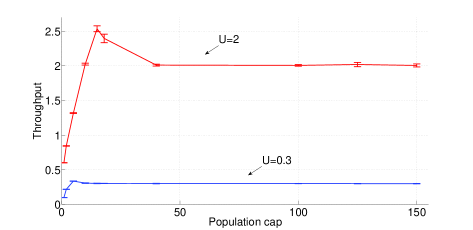
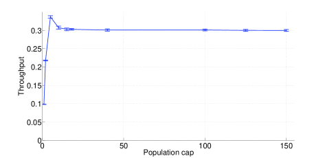
(a) $\mu=\mu^{\prime}=0.5$, and $U\in\{2,0.3\}$

(b) $\mu=\mu^{\prime}=0.5$, and $U=0.3$

Figure 14: Illustrating the benefits of admission control under the MDP/RFB and RUP/RUB policies.

Figure 15 shows the benefits of admission control in the same setting as described above, except that publisher and peers adopt MDP/RFB and RP/RUB policies, respectively. Note that the gains due to admission control are now more pronounced. Still, the asymptotic throughput does not increase substantially when contrasted against Figure 14. When $U=0.3$, the competition between the publisher and the one-club to serve newcomers is responsible for the asymptotic throughput remaining close to $U$. When $U=2$, the peer arrival rate, set to $\lambda=6$, is not large enough to make the server use all its capacity to serve newcomers. In this setting, we observe that roughly 30% of the server bandwidth is devoted to newcomers, whereas the remainder is used to serve the one-club. If we increase the arrival rate to $\lambda=60$, in contrast, we obtain a throughput of 6.67 $\pm 0.0908$, for a population cap of 200 peers. In the latter case, virtually all the service capacity of the server is used to serve newcomers and, as discussed in Section 4.4.1, it should come with no surprise that the obtained throughput is larger than $\lambda_{S}=KU$ due to the effects of admission control.

The results in this section indicate the importance of the core strategies introduced in this paper, namely the adoption of MDP/RUB (resp., RP/RUB) by the server (resp., the peers), the reduction of the service capacity of the one-club, the shielding newcomers and admission control. Under different settings presented above, disabling any of these mechanisms may have detrimental effects on performance.

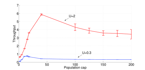
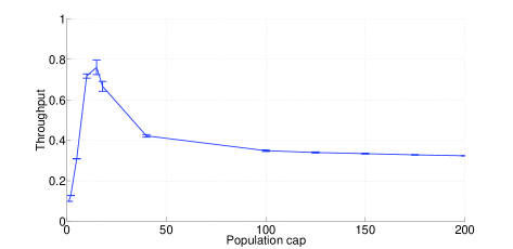
(a) $\mu=\mu^{\prime}=0.5$, and $U\in\{2,0.3\}$

(b) $\mu=\mu^{\prime}=0.5$, and $U=0.3$

Figure 15: Illustrating the benefits of admission control under the MDP/RFB and RP/RUB policies.

6 Related Work

There is a vast literature on the stability and throughput of peer-to-peer swarming systems focusing on its relations with multiple swarms and bundling [46, 10, 48], self-sustainability [7], real-time content dissemination [45, 3], coding [40] and system design [1, 18, 25, 33, 46, 4]. Nonetheless, we were unable to find any previous work that accounted for the missing piece syndrome when computing the throughput of peer-to-peer swarming systems.

In this paper, a number of illustrative results considered small swarms with less than one hundred peers. In some cases, we indicated that such small number of peers suffices to reach the swarm asymptotic throughput. In addition, it has been reported in related work that swarms with small populations are common in the wild. According to [10], most of the swarms are very small: approximately 73% of the swarms measured by [10] are formed by less than 10 peers and 58% have less than 5 peers.

In previous works, authors assumed that either peers and publishers adopted random-peer selection [32], files had at most two blocks [31] or swarming systems behaved differently as compared to the system analyzed in this paper [22]. The most-deprived peer selection policy was first proposed by Bonald et al. [5]. As indicated in this paper, if the publisher adopts the most-deprived peer selection strategy, the throughput of the swarm can increase even if the remaining peers do not change their strategies.

Yang and de Veciana were the first to consider a closed system to analyze the transient increase in throughput after a flash crowd [42]. They also considered an idealized fluid model to study the steady state. In their seminal paper, Yang and de Veciana did not account for the fact that a block might become rare and its retrieval turn into a system bottleneck.

In the peer-to-peer literature, fluid models have been traditionally used to study system performance [24, 35, 39, 13, 14, 15, 2] and scheduling strategies [43]. The importance of taking into account the fact that the file is divided into finite blocks rather than considering the fluid limit was indicated in [25, 46], who discovered that under the Markovian framework introduced by Massoulié and Vojnovic [24] the free random distribution of file pieces suffers from the so called missing piece syndrome. Note that, for tractability purposes, Massoulié and Vojnovic [24] considered a model with built in symmetries across peers. Then, Hajek and Zhu [46] showed that when seeding rate is scarce, symmetry breaking occurs. Such symmetry breaking plays a key role in the system, leading to one piece becoming very rare. In this paper, we also account for this symmetry breaking and its consequences.

The missing piece phenomenon can be avoided by the presence of a sufficient number of seeds, but this solution requires some altruism of peers in the form of staying in system after completing their own downloads (see Section 7). It is an important challenge to find fully distributed protocols that would guarantee stability even with non-altruistic peers. Reittu [37] invented the first one, which was later proven to work [33]. None of those works focused on assessing system throughput. In this paper, we compute the throughput of swarming systems accounting for the fact that the file is divided into finite blocks, and use our model to motivate novel scheduling strategies.

Paganini and Ferragut [13] combined M/M/$\infty$ and M/M/1 queues to model the download progress in P2P networks. The former captures the self-scaling characteristics of the system, while the latter is used to model the over-provisioned regime wherein peers quickly download the file and leave the system before having a chance to cooperate with other peers. In this paper, in contrast, we also combine M/M/$\infty$ and M/M/1 queues, but differently from [13] we use the latter to characterize the under-provisioned regime wherein the publisher becomes the system bottleneck.

Scheduling strategies to improve system throughput usually rely on some sort of altruism. To improve system throughput, in previous works it has been proposed that peers reside in the system after completing their downloads [46], barter for content that they were not interested in [46] or refrain from taking advantage of all contact opportunities [33]. Similar in spirit, in [4] the authors propose a provably-stable incentive-compatible strategy, group suppression, which prevents the increase of the one-club. The idea consists of temporarily refraining certain peers from uploading blocks. In [36], the authors propose a variation of group suppression, referred to as mode suppression, wherein peers may suppress the transmission of the most popular piece. Whereas group suppression is proven to be stable for files with up to three blocks [4], in [36] the authors prove that mode suppression is stable for any number of blocks. In this paper, we show that a simple and incentive-compatible strategy, which consists of reducing the service capacity of the peers that have all but one block, can significantly improve system throughput. An experimental reality check supporting the improvement in system throughput is reported in [28].

It is well known that in swarming systems non work-conserving strategies may perform better than work-conserving ones [43]. In essence, group suppression, mode suppression and capacity throttling are different incarnations of non work-conserving strategies. The authors of [36] identify an interesting open problem, which consists of determining, among non work-conserving strategies, those that minimize sojourn time for stable protocols. We envision that the throughput results obtained with the models presented in this paper constitute a first step towards a better understanding of the impact of piece and peer selection strategies on sojourn times.

7 Assumptions and Limitations

Next, we discuss the key simplifying assumptions adopted in this paper, and some of the related limitations.

Constant peer arrival rate: in the proposed open system model, we assume that peers arrive according to a Poisson process with constant arrival rate. For contents whose arrival rates vary over time, the constant arrival rate approximation must be applied at short windows of time. In a number of scenarios of interest, the steady state throughput is reached after a few peers leave the system (see Section 4.4.2), allowing us to rely on asymptotic values when analyzing the throughput over finite time intervals.

Constant peer mean upload capacity: in most of our analysis and simulations we assumed a constant mean upload capacity. It is straightforward to adjust our simulations to account for a distribution of upload capacities across peers. In [6], the authors considered an analytical model embracing heterogeneous upload capacities. Nonetheless, they did not account for the missing piece syndrome. Our aim here, in contrast, is to provide a simple model that accounts for the missing piece syndrome. Accounting together for the missing piece syndrome and heterogeneous upload capacities would make the model more complex, and as in any modeling framework we need to trade between simplicity and generality.

Peer pairing occurs uniformly at random: peer pairing in real BitTorrent involves a number of mechanisms, including tit-for-tat (TFT). In this paper, to simplify the analysis we ignore those mechanisms and consider the simplest possible peer pairing, which is uniform at random. Still, experimental results indicate that the insights obtained through the simplified model are reflected in emulated experiments using the real Bittorrent client [28].

Push or pull strategies: we assume that the mean time between contacts of peers for opportunities to upload a packet (i.e. push) are characterized by the mean time to upload a block. Alternatively, the model wherein peers contact others for opportunities to download a block (i.e. pull) is mathematically equivalent to the one considered in this paper, as further discussed in [17]. In the two cases, we assume that the contact itself is instantaneous, as the upload or download rates are captured through the time between contacts. By assuming that pairing among peers occurs uniformly at random, most control information flows between peers and the publisher together with the tracker.

Scalability of peer selection policies: next, we indicate simple strategies that may increase the scalability of publisher decisions. Consider a publisher that adopts random useful peer selection, most deprived peer selection or random useful block selection. Newcomers are, by definition, most deprived. If newcomers favor contacts with the publisher, they will naturally simplify the coordination required by the publisher to prioritize transfers of useful blocks to useful peers or to most deprived peers. In particular, we envision that in scenarios of practical interest most gains obtained by the use of most deprived peer selection are due to new peers being prioritized, and actually book-keep how many blocks each peer owns is not necessary. A detailed analysis of that matter is out of the scope of this paper.

Scalability of block selection policies: strict rarest first block selection is typically not scalable and BitTorrent users sample their neighbors to identify the rarest block across a neighborhood. In a swarm wherein the missing piece syndrome is present, it should be straightforward to determine the missing piece (rarest block). In any case, selecting the rarest block out of the neighboring peers should suffice in a number of scenarios of practical interest [21], in particular if peers can count on network coding [30].

Peers leave immediately after completing downloads: in BitTorrent, there are no incentives for peers to remain in the system after completing their downloads. In essence, making swarms independent from each other builds scalability and robustness but precludes incentives for cooperation across swarms after peers complete their downloads. Cooperation across swarms requires some sort of mechanism to translate contributions in a swarm into rewards in another, which would cause interdependencies among swarms and breaking their self-sustaining nature. We briefly analyze the system accounting for peers that altruistically linger as seeds in Appendix F.1.

Peer churn: we assume that peers remain in the system before completing their downloads. If peers have a deadline and leave the system in case their downloads do not complete by the deadline, the one-club does not grow unboundedly and the system is always stable. We briefly analyze the system accounting for peers that may abandon the system before completing their downloads in Appendix F.2.

Usefulness of shielding newcomers: our numerical results indicate that the shielding of newcomers is unnecessary when the effective service capacity of the server is larger than peer capacity. The effective service capacity is the capacity dedicated to a swarm. The effective capacity of the server may be small, for instance, when the server is serving a multitude of swarms, as opposed to serving only a few swarms. In addition, focusing exclusively on the case wherein publishers have large capacity goes counter the idea that anyone can publish content using Bittorrent. Home users, for instance, may have small servers and we envision that the shielding of newcomers may be particularly helpful in those scenarios. According to [34], around 70% of peers have uplink capacity smaller than 100 KB/s.

8 Conclusions

Due to their ability to scale, robustness and efficiency, P2P systems are responsible for a significant portion of today’s Internet traffic and constitute the basis for new architectures such as content centric networking [19]. Although P2P systems are very popular, their fundamental limitations are yet to be fully understood. In particular, the throughput of such systems can be impacted by the missing piece syndrome, but that effect has not been considered in previous works.

In this paper, we present new results to quantify the throughput of P2P systems when the effective service capacity of the publisher is small compared to the arrival rate of peers. We evaluate the impact of different system parameters and system strategies on attainable throughput through the use of models. Using those models, we derive a new upper bound on the throughput achieved when the publisher adopts most deprived peer selection and rarest-first block selection. Our models also suggest a new very simple and incentive-compatible policy, wherein peers reduce their service capacity when they possess all blocks but one. By employing this upload throttling policy, the system can accommodate more users while remaining stable, specially when near saturation.

One of the ultimate goals of P2P swarming systems is to support very high loads (e.g., flash crowds) counting with scarce service capacity from publishers (e.g., home users). This, in turn, is the setup wherein the missing piece syndrome is most likely to occur. Experimental results recently indicated that the missing piece syndrome may indeed occur in real BitTorrent swarms [28]. In this paper, we complement the experimental evidence presented in [28] with a foundational theory to assess the factors that impact swarm throughput under the missing piece syndrome. Taken together, we believe that these works advance the state of the art towards understanding the fundamental limitations of P2P swarming systems and achieving feasible throughput goals.

9 Acknowledgments

E. de Souza e Silva, Rosa M. M. Leão and Daniel S. Menasché are partially supported by grants from CNPq, FAPERJ and FAPESP. Don Towsley is partially supported by grants from NSF.

Appendices

Appendix A Open System Throughput

Our goal in this appendix is to show how system throughput varies as a function of arrival rate, as predicted by the open queueing network model. Figures 16 and 17 show system throughput as a function of the peer arrival rate, for $K=3,U=0.3,\mu=\mu^{\prime},\mu\in\{0.3,0.5,1.0,10.0\}$. We used the queueing network model of Section 3.2, with 4 queues, to obtain the results plotted in the figures. As discussed in Section 3, when considering 4 queues we get rid of $F_{2}$ and $G_{2}$ in Figure 3, and queue $G_{3}$ corresponds to gifted peers that have 2 blocks.

With 4 queues, the queueing network model comprises the following set of equations

$$\lambda_{0} =\lambda$$ (21)

$$\lambda_{1} =\gamma_{p}(0)=\mathbb{E}[n_{0}]\mu$$ (22)

$$\pi_{0}(i)^{-1} =\sum_{s=0}^{\infty}\lambda_{i}^{s}\left(\prod_{l=1}^{s}(U+\mu l)\right)^{-1},\quad i\in\{0,1\}$$ (23)

$$\pi_{s}(i) =\pi_{0}(i)\lambda_{i}^{s}\left(\prod_{l=1}^{s}(U+\mu l)\right)^{-1},\quad i\in\{0,1\}$$ (24)

$$\gamma_{r}(i) =U(1-\pi_{0}(i))\left(\prod_{l=0}^{i-1}\pi_{0}(l)\right),\quad i\in\{0,1\}$$ (25)

$$\mathbb{E}[n_{i}] =\sum_{l=0}^{\infty}\pi_{l}(i)l,\quad i\in\{0,1\}$$ (26)

$$\Gamma =U+2\gamma_{r}(0)+\gamma_{r}(1)$$ (27)

(23)-(24) correspond to the steady-state solution of the birth-death processes associated with queues $F_{0}$ and $F_{1}$, with corresponding arrival rates $\lambda_{0}$ and $\lambda_{1}$, while the additional equations are taken directly from Section 3. The set of equations above is solved given $\lambda$ and $\mu$. First, (23)-(26) are evaluated for $i=0$, then for $i=1$, and finally (27) is evaluated.

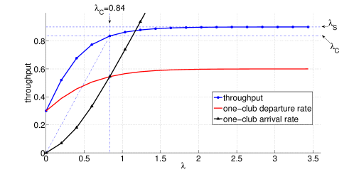
(a)

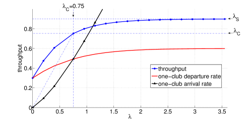
(b)

Figure 16: System throughput: $K=3$, $U=0.3$, (a) $\mu=0.3$ and (b) $\mu=0.5$

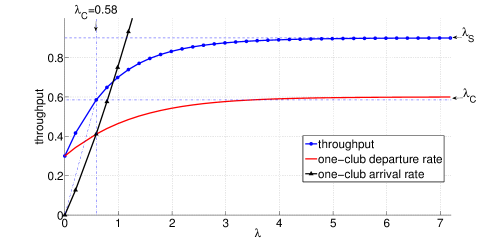
(a)

(b)

Figure 17: System throughput: $K=3$, $U=0.3$, (a) $\mu=1.0$ and (b) $\mu=10.0$

When searching for $\lambda_{C}$, we solve (21)-(27) with the additional constraint $\lambda=\Gamma$. To this aim, we search for the solution using the nonlinear interior-reflective Newton method described in [8], and implemented by the lsqnonlin function in MATLAB. Alternatively, the value of $\lambda_{C}$ is inferred by increasing $\lambda$, computing the corresponding throughput $\Gamma$, and searching for the critical value for which $\lambda=\Gamma$.

Note that the departure rate from the one-club is given by $\mu\mathbb{E}[m_{1}+m_{3}]+U\pi_{0}(0)\pi_{0}(1)=2\gamma_{r}(0)+\gamma_{r}(1)+U\pi_{0}(0)\pi_{0}(1)$, while the arrival rate to the one club is given by $(\lambda-(1-\pi_{0}(0))U)-U\pi_{0}(0)(1-\pi_{0}(1))=\lambda-U(1-\pi_{0}(0)\pi_{0}(1))$. In the figures, the blue line (marked with circles) corresponds to the system throughput (eq. (27)), the red line (plain line) corresponds to the arrival rate of peers to the one-club, and the black line (marked with triangles) corresponds to the departure rate of peers from one-club.

In Figures 16 and 17 the system throughput converges to $KU$. When $\lambda=0$, throughput equals $U$, due to departures from the one-club. As $\lambda$ increases, throughput increases due to the collaboration between peers. In this region ($\lambda<\lambda_{C}$), the departure rate from the one-club is larger than the arrival rate to the one-club, which favors a reduction in the one-club size. When $\lambda=\lambda_{C}$, we observe that the one-club departure and arrival rates equal each other, i.e., the black curve (arrival rate of peers to the one-club) crosses the red curve (departure rate of peers from the one-club) when $\lambda=\lambda_{C}$. For $\lambda>\lambda_{C}$, the throughput still increases until saturation. When $\lambda=\infty$, the throughput equals $\lambda_{S}=KU$.

Comparing Figures 16 and 17, we observe that as $\mu$ increases $\lambda_{C}$ decreases. This is because we are assuming $\mu=\mu^{\prime}$. An increase in the service capacity of peers causes a decrease in the residence time of gifted peers, which in turn contributes to a reduction in the departure rate from the one-club.

Appendix B Iterative Fixed Point Algorithm To Compute $\Gamma_{C}$

Next, we present an iterative process to approximate the critical throughput attained by the population of peers. The process consists of increasing the arrival rate up to reaching its critical value. Let $\Gamma^{(i)}$ and $\lambda^{(i)}$ be the value of $\Gamma$ and $\lambda$ computed at the $i$-th iteration.

Assume that the arrival rate at the first iteration $\lambda^{(0)}$ is given. The steady state solution for queue $F_{0}$ is obtained by constructing a simple birth-death process with parameter values dependent on $U$ and $\mu^{\prime}$. After computing $\mathbb{E}[n_{0}]$ and $\mathbb{P}(n_{0}=0)=\pi_{0}(0)$, equations (2) and (3) yield the arrival rates to queues $G_{1}$ and $F_{1}$, respectively. Similarly, arrival rates to the remaining queues are computed using (5) and (6), and system departure rate $\Gamma^{(0)}$ is determined using (11). Then, we let $\lambda^{(1)}=\Gamma^{(0)}$ and repeat the process. The final solution is obtained by iterating

$$\lambda^{(n)}=\Gamma^{(n-1)}$$ (28)

until convergence is achieved. Let $\tilde{n}$ be the minimum value for which $\lambda^{(\tilde{n})}=\Gamma^{(\tilde{n}-1)}$. Then,

$$\lambda_{C}=\lambda^{(\tilde{n})}$$ (29)

Appendix C Alternative Derivations of $\Gamma_{S}$

C.1 Flow Dynamics

The simple result presented in Proposition 4.1 can also be directly obtained by observing the flow dynamics shown in Figure 2. Recall that based on Figure 2 we derived an upper bound on the system throughput, given by (1). Setting $p=1$ in  (1) we obtain Proposition 4.1.

It is worth contrasting the simple flow dynamics diagram in Figure 2 with the queueing network model in Figure 3. The two leftmost boxes in Figure 2 are captured by queue $F_{0}$. The remaining two boxes in the bottom layer in Figure 2, in turn, are captured by queues $G_{1}$, $G_{2}$ and $G_{3}$ in Figure 3. As indicated above, the expressions for $\Gamma_{S}$ obtained using Figures 2 and 3 are in agreement with each other.

C.2 Mean Field Approximation

Next, we consider a deterministic mean field fluid approximation to the queueing network model. The approach is similar, for instance, to the one considered by Qiu and Srikant [35], which was also influenced by a Markov model [11].

Let $x_{i}(t)$ (resp., $y_{i}(t)$) be the number of peers at queue $F_{i}$ (resp., $G_{i}$). Let $\eta_{i}$ be the fraction of peers from queue $F_{i}$ that are served by the one-club, i.e., $1-\eta_{i}$ is the fraction of peers from queue $F_{i}$ that move to queue $G_{i+1}$, $i=0,1,2,\ldots,\tilde{K}-2$. To simplify presentation, we consider the truncated model with $\tilde{K}=4$ (extension for larger values of $\tilde{K}$ is straightforward). For $\tilde{K}=4$, the fluid model is given by

$$\frac{dx_{0}}{dt} = \lambda-x_{0}\mu^{\prime}-UI(x_{0}>0)$$ (30)

$$\frac{dx_{1}}{dt} = (x_{0}\mu^{\prime}+UI(x_{0}>0))\eta_{0}-(x_{1}\mu^{\prime}+UI(x_{0}=0,x_{1}>0))$$ (31)

$$\frac{dx_{2}}{dt} = (x_{1}\mu^{\prime}+UI(x_{0}=0,x_{1}>0))\eta_{1}-(x_{2}\mu^{\prime}+UI(x_{0}=0,x_{1}=0,x_{2}>0))$$ (32)

$$\frac{dy_{1}}{dt} = (x_{0}\mu^{\prime}+UI(x_{0}>0))(1-\eta_{0})-y_{1}\mu^{\prime}$$ (33)

$$\frac{dy_{2}}{dt} = (x_{1}\mu^{\prime}+UI(x_{0}=0,x_{1}>0))(1-\eta_{1})+y_{1}\mu^{\prime}-y_{2}\mu^{\prime}$$ (34)

$$\frac{dy_{3}}{dt} = (x_{2}\mu^{\prime}+UI(x_{0}=0,x_{1}=0,x_{2}>0))(1-\eta_{2})+y_{2}\mu^{\prime}-y_{3}\frac{\mu^{\prime}}{K-3}$$ (35)

The mean field approximation is obtained from the fluid model replacing the joint event denoting that queues $F_{0},\ldots,F_{j-1}$ are empty, and queue $F_{j}$ is non-empty, $I(\cap_{l=0}^{j-1}\{x_{l}=0\},\{x_{j}>0\})$, by the corresponding product of probabilities $\prod_{l=0}^{j-1}\pi_{0}(l)(1-\pi_{0}(j))$ (see also Section 3). In the saturated regime, we have $\pi_{0}(0)=0$. In steady state, and under saturation,

$$\eta_{0}=\frac{\lambda-U}{\lambda},\eta_{1}=\eta_{2}=1,\quad x_{0}=x_{1}=x_{2}=\frac{\lambda-U}{\mu^{\prime}},\quad y_{1}=y_{2}=\frac{U}{\mu^{\prime}},y_{3}=(K-3)\frac{U}{\mu^{\prime}}$$ (36)

System throughput is given by

$$\Gamma_{S} =\mu\left(y_{1}+y_{2}\right)+\left(\frac{K-4}{K-3}\ \mu+\frac{1}{K-3}\mu^{\prime}\right)y_{3}+U$$ (37)

$$=(2+(K-4))\mu U/\mu^{\prime}+2U$$ (38)

$$=\left(\frac{(K-2)\mu}{\mu^{\prime}}+2\right)U$$ (39)

The first term in (37) corresponds to departures due to service from peers in queues $G_{1}$ and $G_{2}$ to peers in the one-club. Peers in $G_{1}$ and $G_{2}$ serve at rate $\mu$. The second term in (37) corresponds to the departures due to services from peers in queue $G_{3}$. A fraction $({K-4})/({K-3})$ of those peers serve at rate $\mu$, whereas the remaining fraction serves at rate $\mu^{\prime}$. The third term corresponds to the departures of gifted peers. After algebraic manipulation, the resulting expression (39) equals (18).

Appendix D Markov Model Details

We model a swarm as a continuous-time Markov chain with state space $\Omega$ and infinitesimal generator $Q$. Let $\mathcal{F}=\{1,\ldots,K\}$ and $\mathcal{C}$ be the set of subsets of $\mathcal{F}$.

Each user has a signature, defined as a set containing element $i$ if the user has block $i$ and 0 otherwise, $i=1,2,\ldots,K$. As users leave the system as soon as they obtain their last block, each user has one of $2^{n}-1$ signatures.

Let $\sigma_{C}$ be the number of peers with signature $C$, where $C\in\mathcal{C}\setminus\mathcal{F}$. State ${\mbox{\boldmath$\sigma$}}\in\Omega$ is characterized by the number of users with each signature, ${\mbox{\boldmath$\sigma$}}=(\sigma_{\emptyset},\sigma_{\{1\}},\ldots,\sigma_{\mathcal{F}\setminus\{K\}})$. Note that it is possible to lump the state space, but to simplify presentation in this appendix we consider the unlumped state space. Let ${\bf e}_{C}$ denote the vector with the same dimension as $\sigma$, with a one in position $C$ and other coordinates equal to zero.

Let $\Gamma_{s}(C,C^{\prime})$ and $\Gamma_{p}(C,C^{\prime})$ be the aggregate transition rate of peers of type $C$ to type $C^{\prime}$ due to service from the server and from other peers, respectively. We assume peers adopt the random peer, random useful block selection, whereas the publisher strategy is varied. In some cases, it will be convenient to make explicit the block which is received by a peer with signature $C$, replacing $C^{\prime}$ by $C^{\prime}_{j}$ when block $j$ is received. After a peer with signature $C$ receives block $j$, $j\notin C$, the number of peers with signature $C^{\prime}_{j}$ increases by one. Recall that as soon as peer completes its download a new one arrives (closed system). Then,

$$C^{\prime}_{j}=\left\{\begin{array}[]{ll}C\cup\{j\},&\textrm{if }|C|<K-1\\ \emptyset,&\textrm{otherwise}\end{array}\right.$$ (40)

Next, we characterize the positive elements of $Q$. When a peer that has all blocks except $j$ gets block $j$, its signature transitions from $\mathcal{F}\setminus\{j\}$ to $\mathcal{F}$. Then, it immediately leaves the system and another peer, with signature $\emptyset$, arrives. Then, the rate at which the system transitions from state $\sigma$ to ${\mbox{\boldmath$\sigma$}}-{\bf e}_{\mathcal{F}\setminus\{j\}}+{\bf e}_{\emptyset}$ is,

$$q_{{\mbox{\boldmath$\sigma$}},{\mbox{\boldmath$\sigma$}}-{\bf e}_{\mathcal{F}\setminus\{j\}}+{\bf e}_{\emptyset}}=\Gamma_{s}(\mathcal{F}\setminus\{j\},\emptyset)+\Gamma_{p}(\mathcal{F}\setminus\{j\},\emptyset),\textrm{ for }j=1,2,\ldots,K$$ (41)

When a peer that needs more than one blocks gets block $j$, its signature transitions from $C$ to $C\cup\{j\}$. The corresponding rate at which the system transitions from state $\sigma$ to state ${\mbox{\boldmath$\sigma$}}-{\bf e}_{C}+{\bf e}_{C\cup\{j\}}$ is

$$q_{{\mbox{\boldmath$\sigma$}},{\mbox{\boldmath$\sigma$}}-{\bf e}_{C}+{\bf e}_{C\cup\{j\}}}=\Gamma_{s}(C,C\cup\{j\})+\Gamma_{p}(C,C\cup\{j\}),\textrm{ for all }C\in\mathcal{C},|C|<K-1$$ (42)

Let $\pi_{\sigma}$ be the steady state probability of state $\sigma$. The vector of steady state probabilities is denoted by $\pi$.

Let $\lambda$ be the throughput of the Markov model. The throughput is given as a function of $q_{{\mbox{\boldmath$\sigma$}},{\mbox{\boldmath$\sigma$}}-{\bf e}_{\mathcal{F}\setminus\{j\}}+{\bf e}_{\emptyset}}$ as follows,

$$\lambda=\sum_{\sigma\in\Omega}\sum_{j=1}^{K}\pi_{\sigma}q_{{\mbox{\boldmath$\sigma$}},{\mbox{\boldmath$\sigma$}}-{\bf e}_{\mathcal{F}\setminus\{j\}}+{\bf e}_{\emptyset}}$$ (43)

Let $\mathcal{N}^{\prime}_{S}$ be the set of neighbors of each of the peers with signature $S$, $i.e.,$ the candidate peers to which a peer with signature $S$ can potentially transfer content. Except otherwise noted, we assume $|\mathcal{N}^{\prime}_{S}|=N-1$.

Let $\mu_{S}$ be the service capacity of peers with signature $S$. When considering homogeneous peers, we let $\mu_{S}=\mu$ for all $S\in\mathcal{C}$. When studying the special policy wherein peers with all blocks except one reduce their service capacity to $\mu^{\prime}$, we let $\mu_{S}=\mu$ if $|S|<K-1$ and $\mu_{S}=\mu^{\prime}$ if $|S|=K-1$.

For $C\in\mathcal{C}$ and $j=1,2,\ldots,K$, we have

$$\Gamma_{p}(C,C^{\prime}_{j})=\left\{{\begin{array}[]{ll}{\sigma_{C}}\left({\sum_{S:j\in S\setminus C}\frac{{\mu}_{S}\sigma_{S}}{|S-C||\mathcal{N}^{\prime}_{S}|}}\right),&j\notin C\\ 0,&\textrm{otherwise}\end{array}}\right.$$ (44)

If the tracker does not announce all newcomers to other peers, equation (44) still holds, except for $C=\emptyset$. In this case, $|\mathcal{N}^{\prime}_{\emptyset}|=N-1$ but $|\mathcal{N}^{\prime}_{C}|\leq N-1$ for $C\neq\emptyset$ (see Section 3).

In what follows, we characterize $\Gamma_{s}(C,C^{\prime})$ for the different strategies considered in this paper,

• random peer, random block: the publisher allocates capacity $U\sigma_{C}/N$ to serve peers with signature $C$, and each of the useful blocks is transferred with same probability. Then,

  $$\Gamma_{s}(C,C^{\prime}_{j})=\left\{\begin{array}[]{ll}\frac{U\sigma_{C}}{N(K-|C|)},&j\notin C\\ 0,&\textrm{otherwise}\end{array}\right.$$ (45)

• random peer, rarest block: let $\mathcal{R}_{C}$ be the set of less replicated blocks among those which are useful for a peer with signature $C$. Then, replacing $K-|C|$ by $|\mathcal{R}_{C}|$ in (45) we obtain

  $$\Gamma_{s}(C,C^{\prime}_{j})=\left\{\begin{array}[]{ll}\frac{U\sigma_{C}}{N|\mathcal{R}_{C}|},&j\notin C,j\in\mathcal{R}_{C}\\ 0,&\textrm{oterwise}\end{array}\right.$$ (46)

• most deprived peer, rarest block: let $\mathcal{M}$ be the set of signatures of most deprived peers. Then, replacing $N$ by $\sum_{C:C\in\mathcal{M}}\sigma_{C}$ in (46) we obtain

  $$\Gamma_{s}(C,C^{\prime}_{j})=\left\{\begin{array}[]{ll}\frac{U\sigma_{C}}{\left(\sum_{C:C\in\mathcal{M}}\sigma_{C}\right)|\mathcal{R}_{C}|},&C\in\mathcal{M},j\notin C,j\in\mathcal{R}_{C}\\ 0,&\textrm{otherwise}\end{array}\right.$$ (47)

Appendix E Lumped Model Details

We present the algorithm used to generate the lumped state space. Algorithm 1 takes as input a state of the unlumped state space, and generates as output the corresponding state in the lumped version of the model. To this aim, it sorts the block according to their number of replicas (line 1), and reorders the block identifiers based on this ordering (line 4). The new signatures are generated (line 12) and the new state is computed (line 15).

Note that the number of states in the unlumped version of the model is ${2^{K}-2+N\choose N}$, $i.e.$, the number of ways of dividing $N$ indistinguishable users into $2^{K}-1$ groups, where each group corresponds to a signature. The number of states in the lumped model is up to an order of magnitude smaller than the number of states in the unlumped model. For instance, for $K=3$ and a population of $N=20$ users, lumping decreases the number of states from 230,230 to 46,163 (see Table 5).

Algorithm 1 LumpState

0:  state $\sigma$ in unlumped state space $\Omega$

0:  state ${\mbox{\boldmath$\sigma$}}^{\prime}$ in lumped state space $\Omega^{\prime}$

1:  $s\leftarrow$ list of block identifiers, sorted by number of replicas

2:  $i\leftarrow 1$

3:  while $i\leq K$ do

4:     $n(s(i))\leftarrow i$, $i\leftarrow i+1$

5:  end while

6:  $\mathcal{C}\leftarrow$ set of subsets of $\{1,\ldots,K\}$

7:  $\mathcal{C}\leftarrow\mathcal{C}\setminus\{\mathcal{F}\}$

8:  while $\mathcal{C}\neq\emptyset$ do

9:     remove signature $C$ from $\mathcal{C}$, $C^{\prime}\leftarrow\emptyset$

10:     $j\leftarrow 1$

11:     while $j\leq K$ do

12:       if ($j\in C$) $C^{\prime}\leftarrow C^{\prime}\cup\{n(j)\}$

13:       $j\leftarrow j+1$

14:     end while

15:     $\sigma^{\prime}_{C^{\prime}}\leftarrow\sigma_{C}$

16:  end while

17:  output ${\mbox{\boldmath$\sigma$}}^{\prime}$ is the lumped state

$$\begin{array}[]{l|l|l}\hline\cr\textrm{number of peers ($N$)}&\textrm{number of states }&\textrm{number of states }\\ &\textrm{(lumped model)}&\textrm{(unlumped model)}\\ \hline\cr 5&127&462\\ 6&243&924\\ 7&429&1716\\ 8&728&3003\\ 9&1174&5005\\ 10&1836&8008\\ 11&2772&12376\\ 12&4086&18564\\ 13&5868&27132\\ 14&8268&38760\\ 15&11418&54264\\ 16&15525&74613\\ 17&20775&100947\\ 18&27445&134596\\ 19&35787&177100\\ 20&46163&230230\\ \hline\cr\end{array}$$

Table 5: File with $K=3$ blocks. Illustrating the gains due to lumping.

Appendix F Delayed and Premature Departures

Next, we consider delayed departures (peers lingering as seeds) and premature departures (peer churn).

F.1 Delayed Departures: Peers Lingering as Seeds

We consider the case where peers remain in the system as seeds after completing their downloads. Let $K=2$, $U=1$ and $\mu=1$. Figure 18(a) shows that when $\gamma\leq 1.2$ the throughput increases linearly as the population increases. In this case, the system is stable, in accordance to  [17]. The situation is not as simple when $\gamma\geq 1.5$. When $\gamma=\infty$, Figure 18(b) shows that the throughput reaches an asymptote when the population grows, for the reasons explained in this paper. It also indicates that if the publisher replaces the random piece policy by the rarest piece policy, the gains are negligible, which again is in accordance to  [17]. For more details about this scenario, refer to [27].

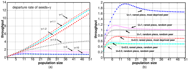
Figure 18: Scalability when peers linger in the system after completing download: $(a)$ peers remain in the system as seeds for an average of $1/\gamma$ after completing download; $(b)$ peers depart immediately.

F.2 Premature Departures: Peer Churn

Next, we consider the scenario wherein peers can prematurely abandon the system before concluding their downloads. First, we consider the simplest setup wherein each peer is equipped with a timer that is started when the peer joins the system and that triggers after a possibly random period of time, with mean $1/\alpha$. If the timer triggers before the download concludes, the peer abandons the system. In this case, the system is stable, and the one club is bounded. The missing piece syndrome will not occur, as the mean number of peers in the system is bounded by $\lambda/\alpha$.

Now, consider the case where peers can decide to abandon the system immediately after completing the download of a block (any block). In addition, to simplify notation we assume that gifted peers do not prematurely abandon the system. Indeed, such peers have less incentives to prematurely abandon the system than their non-gifted counterparts. Because the gifted peers possess the rarest block, their download progresses smoothly unlike the non-gifted peers that may be suffer from very long delays waiting for the rarest block.

After the download of each block, abandonments can be characterized either from a population-wide perspective (wherein the aggregate rate at which the population abandons the system is given) or from an individual peer perspective (wherein the individual probability that a peer abandons the system is given). In what follows, we consider the latter. Let $q_{i}$ be the probability that a peer abandons the system after obtaining its $(i+1)$-th first block. Then, $\gamma_{p}(i)$ is given by (6), multiplying the right hand side by $q_{i}$,

$$\gamma_{p}(i)=\mathbb{E}[n_{i}]\mu^{\prime}q_{i}.$$ (48)

All the remaining equations in Sections 3.2 and 3.3 and Proposition 4.1 still hold.

Recall that in Proposition 4.1 the saturation throughput is the maximum throughput achievable by the open system. Let $\tilde{q}$ be the probability that a peer prematurely abandons the system. If $(\lambda-U)(1-\tilde{q})>\left(\frac{(K-2)\mu}{\mu^{\prime}}+1\right)U$ the arrival rate to the one-club is larger than the corresponding departure rate (Figure 2), the one-club still grows unboundedly and the arguments presented in Section 4.3.1 remain valid to derive (18).

Appendix G Additional Policies

Most of the throughput analysis in this paper focused on a publisher adopting the most deprived peer/rarest-first block policy. Next, we consider two additional policies. We still assume that peers adopt the random peer/random block policy (RP/RB).

G.1 MDP/RB

The analysis of most deprived peer/random block policy by publishers is similar to the one presented under the flow dynamics in Section 3. The key difference consists of the rate of newcomers that become gifted, which must be replaced from $pU$ by $pU/K$. Similarly, in the queueing network model the rates $\gamma_{r}(i)$ must be multiplied by $1/K$. It can be verified that the maximum throughput capacity, when $\mu=\mu^{\prime}$, equals $U$, i.e., the benefits of MDP do not hold if the publisher adopts RB in place of RFB.

G.2 RP/RB with seeds

Next, we consider peers that remain in the system after completing their downloads. The flow dynamics analysis in Section 3 can be extended to allow for peers that remain in the system as seeds after completing their downloads. We consider a publisher that adopts RP/RB.

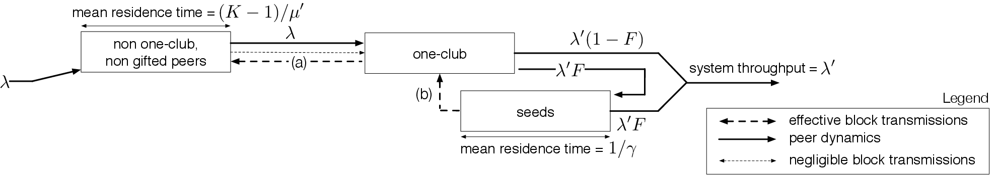
Figure 19: Flow dynamics with seeds

The flow dynamics is shown in Figure 19. Let $\lambda^{\prime}$ be the rate at which peers leave the one-club. It follows from Little’s result that there are on average $\lambda^{\prime}F/\gamma$ seeds in the system. Each seed serves at rate $\mu^{\prime}$. Then, in steady state we have $\Gamma=\lambda^{\prime}=\min(\lambda,U+\lambda^{\prime}F\mu^{\prime}/\gamma)$. Equivalently,

$$\lambda^{\prime}=\min\left(\lambda,\frac{U}{1-\mu^{\prime}F/\gamma}\right)$$ (49)

Note that the equation above holds if $F\mu^{\prime}/\gamma\leq 1$. In particular, if $1/\gamma=1/(F\mu^{\prime})$ we have $\lambda=\lambda^{\prime}$ and peers will experience bounded delays. If $1/\gamma>1/(F\mu^{\prime})$, delays are further reduced as peers count with the assistance of additional seeds.

Note that a slightly more restricted version of this result has already been proved in [47]. Here, we illustrate the simplicity of the flow balance dynamics to derive this and similar results.

References

- [1] E. Altman, P. Nain, A. Shwartz, and Y. Xu. Predicting the impact of measures against p2p networks: transient behavior and phase transition. TON, 21(3):935–949, 2013.
- [2] Nasreen Anjum, Dmytro Karamshuk, Mohammad Shikh-Bahaei, and Nishanth Sastry. Survey on peer-assisted content delivery networks. Computer Networks, 2017.
- [3] F. Baccelli, F. Mathieu, I. Norros, and R. Varloot. Can p2p networks be super-scalable? In IEEE INFOCOM, 2013.
- [4] Omer Bilgen and Aaron B. Wagner. A New Stable Peer-to-Peer Protocol with Non-Persistent Peers. In IEEE INFOCOM, 2017.
- [5] T. Bonald, L. Massoulié, F. Mathieu, D. Perino, and A. Twigg. Epidemic live streaming: optimal performance trade-offs. In SIGMETRICS, volume 36, pages 325–336. ACM, 2008.
- [6] A. Chow, L. Golubchik, and V. Misra. Bittorrent: An extensible heterogeneous model. In INFOCOM, pages 585–593, 2009.
- [7] D. Ciullo, V. Martina, M. Garetto, E. Leonardi, and G. Torrisi. Stochastic analysis of self-sustainability in peer-assisted vod systems. In IEEE INFOCOM, pages 1539–1547, 2012.
- [8] Thomas F Coleman and Yuying Li. An interior trust region approach for nonlinear minimization subject to bounds. SIAM Journal on optimization, 6(2):418–445, 1996.
- [9] E. de Souza e Silva, R.M. Leão, and D. R. Figueiredo. An integrated modeling environment for computer systems and networks. Performance Evaluation Review, 36(4):64–69, 2009.
- [10] E. de Souza e Silva, R.M.M. Leão, D.S. Menasché, and A.A. Rocha. On the interplay between content popularity and performance in P2P systems. In QEST, pages 3–21. Springer, 2013.
- [11] G. de Veciana and X. Yang. Fairness, incentives and performance in peer to peer networks. In Forty-first Annual Allerton Conference on Communication, Control and Computing, 2003.
- [12] B. Fan, D. Chiu, and J. Lui. The delicate tradeoffs in bittorrent-like file sharing protocol design. In ICNP, pages 239–248. IEEE, 2006.
- [13] A. Ferragut and F. Paganini. Fluid models of population and download progress in p2p networks. IEEE Transactions on Control of Network Systems, 3(1):34–45, March 2016.
- [14] Andrés Ferragut and Fernando Paganini. Queueing analysis of peer-to-peer swarms: stationary distributions and their scaling limits. Performance Evaluation, 93:47–62, 2015.
- [15] YV Gaidamaka, EV Bobrikova, and EG Medvedeva. The application of fluid models to the analysis of peer-to-peer network. RUDN Journal of Mathematics, Information Sciences and Physics, 4:15–25, 2016.
- [16] Winfried K Grassmann, Michael I Taksar, and Daniel P Heyman. Regenerative analysis and steady state distributions for Markov chains. Operations Research, 33(5):1107–1116, 1985.
- [17] B. Hajek and J. Zhu. The missing piece syndrome in peer-to-peer communication. In IEEE ISIT, 2010.
- [18] K. Hwang, V. Gopalakrishnan, R. Jana, S. Lee, V. Misra, K. Ramakrishnan, and D. Rubenstein. Joint-family: Enabling adaptive bitrate streaming in p2p video-on-demand. In ICNP, 2013.
- [19] Van Jacobson, D. Smetters, J. Thornton, M. Plass, N. Briggs, and R. Braynard. Networking named content. In CONEXT, pages 1–12. ACM, 2009.
- [20] A. Legout, N. Liogkas, E. Kohler, and L. Zhang. Clustering and sharing incentives in Bittorrent systems. In ACM SIGMETRICS, 2007.
- [21] Arnaud Legout, Nikitas Liogkas, and Eddie Kohler. Rarest first and choke algorithms are enough. In IMC, 2006.
- [22] L. Leskelä, P. Robert, and F. Simatos. Interacting branching processes and linear file-sharing networks. Advances in Applied Probability, 42(3):834–854, 2010.
- [23] Laurent Massoulie and Andrew Twigg. Rate-optimal schemes for peer-to-peer live streaming. Performance Evaluation, 65(11-12):804–822, 2008.
- [24] Laurent Massoulié and Milan Vojnovic. Coupon replication systems. IEEE/ACM Transactions on Networking (TON), 16(3):603–616, 2008.
- [25] Fabien Mathieu and Julien Reynier. Missing piece issue and upload strategies in flashcrowds and p2p-assisted filesharing. In AICT/ICIW, 2006.
- [26] D. S. Menasché, A. A. de A. Rocha, E. de Souza e Silva, D. Towsley, and R. M. M. Leão. Implications of peer selection strategies by publishers on the performance of p2p swarming systems. ACM SIGMETRICS Performance Evaluation Review, 39(3):55–57, 2011.
- [27] Daniel S. Menasché, A.A.A. Rocha, E. de Souza e Silva, Rosa M.M. Leão, and Don Towsley. Stability of peer-to-peer swarming systems. In SBRC, 2012. http://ce-resd.facom.ufms.br/sbrc/2012/ST4_1.pdf.
- [28] Diego Ximenes Mendes, Edmudno de Souza e Silva, Daniel S. Menasché, Rosa Leão, and Don Towsley. An experimental reality check on the scaling laws of swarming systems. In IEEE INFOCOM, 2017.
- [29] F. Murai, A.A. Rocha, D. Figueiredo, and E. de Souza e Silva. Heterogeneous download times in a homogeneous bittorrent swarm. Computer Networks, 56:1983–2000, 2012.
- [30] Di Niu and Baochun Li. Topological properties affect the power of network coding in decentralized broadcast. In INFOCOM, 2010 Proceedings IEEE, pages 1–9. IEEE, 2010.
- [31] Ilkka Norros, Hannu Reittu, and Timo Eirola. On the stability of two-chunk file-sharing systems. Queueing Systems, 67(3):183–206, 2011.
- [32] R. Núnez-Queija and B. Prabhu. Scaling laws for file dissemination in p2p networks with random contacts. In Quality of Service. International Workshop on, pages 75–79. IEEE, 2008.
- [33] B. Oguz, V. Anantharam, and I. Norros. Stable, distributed p2p protocols based on random peer sampling. IEEE/ACM Transactions on Networking, 23(5):1444–1456, October 2015.
- [34] Michael Piatek, Tomas Isdal, Thomas Anderson, Arvind Krishnamurthy, and Arun Venkataramani. Do incentives build robustness in Bittorrent? In 4th USENIX Symposium on Networked Systems Design & Implementation, 2007.
- [35] D. Qiu and R. Srikant. Modeling and performance analysis of bittorrent-like peer-to-peer networks. In SIGCOMM, volume 34, pages 367–378. ACM, 2004.
- [36] Vamseedhar Reddyvari, Parimal Parag, and Srinivas Shakkottai. Mode-suppression: A simple and provably stable chunk-sharing algorithm. In INFOCOM, 2018.
- [37] Hannu Reittu. A stable random-contact algorithm for peer-to-peer file sharing. In International Workshop on Self-Organizing Systems, pages 185–192. Springer, 2009.
- [38] B. Schroeder, A. Wierman, and M. Harchol-Balter. Open versus closed: A cautionary tale. In NSDI, 2006.
- [39] F. Simatos, P. Robert, and F. Guillemin. Analysis of a queueing system for modeling a file sharing principle. In ACM SIGMETRICS, 2008.
- [40] Cedric Westphal. A stable fountain code mechanism for peer-to-peer content distribution. In IEEE INFOCOM, pages 2571–2579, 2014.
- [41] R.L. Xia and J. Muppala. A survey of bittorrent performance. IEEE Communications Surveys & Tutorials, 12(2):140–158, 2010.
- [42] X. Yang and G. de Veciana. Performance of peer-to-peer networks: Service capacity and role of resource sharing policies. Performance Evaluation, 63:175––194, 2006.
- [43] Bo Zhang, Sem C Borst, and Martin I Reiman. Optimal server scheduling in hybrid p2p networks. Performance Evaluation, 67(11):1259–1272, 2010.
- [44] X. Zhou, S. Ioannidis, and L. Massoulié. On the stability and optimality of universal swarms. ACM SIGMETRICS Performance Evaluation Review, 39(1):301–312, 2011.
- [45] J. Zhu and B. Hajek. Tree dynamics for peer-to-peer streaming. arXiv preprint arXiv:1308.1971, 2013.
- [46] Ji Zhu. Stability and performance in peer to peer networks. PhD thesis, University of Illinois at Urbana-Champaign, 2014.
- [47] Ji Zhu and Bruce Hajek. Stability of a peer-to-peer communication system. Information Theory, IEEE Transactions on, 58(7):4693–4713, 2012.
- [48] Ji Zhu, Stratis Ioannidis, Nidhi Hegde, and Laurent Massoulié. Stable and scalable universal swarms. In PODC, pages 260–269. ACM, 2013.