Event-Triggered Stabilization of Linear Systems Under Bounded Bit Rates

Abstract

This paper addresses the problem of exponential practical stabilization of linear time-invariant systems with disturbances using event-triggered control and bounded communication bit rate. We consider both the case of instantaneous communication with finite precision data at each transmission and the case of non-instantaneous communication with bounded communication rate. Given a prescribed rate of convergence, the proposed event-triggered control implementations opportunistically determine the transmission instants and the finite precision data to be transmitted on each transmission. We show that our design exponentially practically stabilizes the origin while guaranteeing a uniform positive lower bound on the inter-transmission and inter-reception times, ensuring that the number of bits transmitted on each transmission is upper bounded uniformly in time, and allowing for the possibility of transmitting fewer bits at any given time if more bits than prescribed were transmitted earlier. We also characterize the necessary and sufficient average data rate for exponential practical stabilization. Several simulations illustrate the results.

I Introduction

The digital nature of communication in networked control systems naturally induces sampling and quantization of signals. The increasing ubiquity of these systems, particularly in resource-constrained domains where communication channels have low, time-varying, and possibly unreliable channel capacity, has brought to the forefront the need for integrated and systematic design methodologies that go beyond adhoc approaches. This paper is a contribution to the modern body of research that seeks to fundamentally address the problem of control under constrained resources. Specifically, we seek to combine the strengths of event-triggered control and information theory to efficiently stabilize linear time-invariant systems under communication constraints.

Literature Review: The need for integration between computing, communication, and control in the study of cyberphysical systems cannot be overemphasized [1, 2]. The present work builds on two areas of research that address the stabilization of control systems under limited information from different and complementary perspectives. In the information-theoretic approach to control under communication constraints, the focus is on determining sufficient and necessary conditions on the bit data rates (i.e., the number of bits transmitted over possibly multiple transmissions during an arbitrary time interval) that guarantee stabilization under varying assumptions on the communication channels. The works [3, 4] provide comprehensive accounts of this by now vast literature, and we highlight next a few references most relevant to the discussion here. Early data rate results appeared in [5, 6, 7], which employ the idea of countering the information generated (the growth in the uncertainty of the system state) with a sufficiently high data rate of the encoded feedback. This approach has been successful in providing tight necessary and sufficient conditions on the data rate of the encoded feedback for asymptotic stabilization in the discrete-time setting. Similar ideas have been used to provide data rate theorems also for stochastic rate channels [8] and extended to vector systems and time-varying feedback channels [9] and Markov feedback channels [10]. In the continuous-time setting, the problem has been mainly studied under either periodic sampling or aperiodic sampling with known upper and lower bounds on the sampling period for single input systems [11, 12], nonlinear feedforward systems [13], and switched linear systems [14]. In this context, it is not known if and how a best sampling period may be designed or if state-based aperiodic sampling can provide any advantage in efficiency and performance. With a few exceptions, see e.g., [14], the works above do not characterize the convergence rates or explore the problem of guaranteeing a desired performance.

Event-triggered control, instead, trades computation and decision-making for less communication, sensing, or actuation effort, while guaranteeing a desired level of performance. This literature, see e.g. [15, 16, 17] and references therein, exploits the tolerance to measurement errors to design goal-driven state-based aperiodic sampling for the efficient use of the system resources. The main focus of this body of work is on minimizing the number of updates while guaranteeing the feasibility of the resulting real-time implementation. When interpreted in terms of communication, this results in a paradigm where one seeks to minimize the number of transmissions while largely ignoring the quantization aspect and allowing the data at each transmission to be of infinite precision. Among the few exceptions, we mention event-triggered schemes with static logarithmic quantization [18, 19] and dynamic quantization [20, 21, 22, 23, 24]. In [18], events are defined as the system state crossing static quantization cells and communication is assumed to be instantaneous and there are no disturbances. [19] considers the problem with modeling errors and communication delays. Both these papers do not explicitly study the notion of communication bit rate (i.e., the number of bits per transmission). In [20, 21, 22, 23], the events are defined as the infinity norm of the encoding error crossing a fixed or piecewise-constant threshold. [20] considers instantaneous communication and external disturbances, although the use of a fixed threshold in the event-triggering condition results in practical stability even under no disturbance. In addition, if the channel imposes a bound on the communication bit rate, then it also affects the ultimate bound on the state. [21] addresses the problem for nonlinear systems and with communication delays, while [22, 23, 24] extend these results to the case with external disturbance. All these works guarantee a positive lower bound on the inter-transmission times, while [20, 21, 22, 23, 24] also provide a uniform bound on the communication bit rate. However, these references do not address the inverse problem of triggering and quantization given a limit on the communication bit rate imposed by the channel. While guarantees on the uniform boundedness of the communication bit rate are useful, they do not characterize either necessary or sufficient conditions on the required data rates, i.e., the number of bits averaged over a finite or infinite time horizon. In fact, this is a shortcoming of the event-triggered control literature as a whole, where the availability of such analytical results would help in the design of networked control systems. Finally, the common underlying approach in the event-triggered literature is based on the notion of input-to-state-stability with respect to measurement errors for both event-triggering and quantization. This is in contrast with the information-theoretic data rate approach to quantization and encoding adopted here.

Statement of Contributions: This paper designs event-triggered controllers for linear-time invariant systems under bounded communication bit rate. We focus on the control goal of exponential practical stabilization, in the presence of disturbance and with a prescribed rate of convergence. The first contribution is the identification of a necessary condition on the average data rate required for all solutions of a linear-time invariant system to exponentially converge with a prescribed convergence rate. Our second set of contributions pertain to the design of event-triggered controllers that guarantee exponential convergence with a desired performance by adjusting the communication rate in accordance with state information in an opportunistic fashion. We consider increasingly realistic scenarios, ranging from instantaneous transmissions with arbitrary, but finite communication rate, through instantaneous transmissions with uniformly bounded communication rate, to finally non-instantaneous transmissions with arbitrary bounded communication rate imposed by the channel. In all cases, our design guarantees the existence of a uniform positive lower bound on inter-transmission and inter-reception times, and ensures that the number of bits transmitted at each transmission is upper bounded. An overarching contribution of the paper is the introduction of the information-theoretic data rate approach to quantization and encoding to complement event-triggering for data rate limited feedback control. From an event-triggered control perspective, our key contribution is going beyond the paradigm of infinite precision at each transmission and adopting the information-theoretic approach to quantization, encoding, and triggering. This allows us to characterize necessary and sufficient data rates averaged over time, and quantify the capability to transmit fewer bits if more bits than prescribed were transmitted earlier. From an information-theoretic perspective, our key contribution is the efficient use of the communication resources by exploiting state-based opportunistic sampling. This allows us to tune the operation of the control system to the desired level of performance and guarantee a desired convergence rate. In order to communicate the main ideas effectively, we use a simple encoding scheme and assume that the encoder and the decoder know the communication delays in the case of non-instantaneous communication. These are aspects that may be improved upon within the framework of the paper. Finally, we believe the approach laid out here opens up numerous avenues for further research at the intersection of information theory, control, and stabilization.

Organization: Section II formally states the asymptotic stabilization problem under event-triggered control and finite communication bit rate. Section III identifies a necessary condition on the average data rate required for all solutions to asymptotically converge with a prescribed convergence rate. Sections IV and V present our event-triggered control design with bounded communication rate under instantaneous and non-instantaneous communication, respectively. Section VI presents simulation results. Finally, Section VII gathers our conclusions and ideas for future work. Proofs of certain auxiliary lemmas are presented in the appendix for smoother readability.

Notation: We let $\mathbb{R}$, $\mathbb{R}_{\geq 0}$, ${\mathbb{N}}$, and ${\mathbb{N}}_{0}$ denote the set of real, nonnegative real, positive integer, and nonnegative integer numbers, respectively. We let $\mathrm{I}_{n}$ and $\mathrm{0}_{n}\in\mathbb{R}^{n\times n}$ denote the identity and zero matrix, respectively, of dimension $n$. For a matrix $A$, let $\sigma_{A}$ denote the spectrum of the matrix $A$ and $\mathrm{Re}({\sigma_{A}})$ denote the set of real parts of the eigenvalues of $A$. For a symmetric matrix $A\in\mathbb{R}^{n\times n}$, we let $\lambda_{m}(A)$ and $\lambda_{M}(A)$ denote its smallest and largest eigenvalues, respectively. For a symmetric positive definite matrix $P\in\mathbb{R}^{n\times n}$ and all $x\in\mathbb{R}^{n}$,

$$\sqrt{\lambda_{m}(P)}\|x\|_{2}\leq\sqrt{x^{T}Px}\leq\sqrt{\lambda_{M}(P)}\|x\|_{2}.$$ (1)

Given $A_{1},A_{2}\in\mathbb{R}^{n\times n}$, $A_{1}\prec A_{2}$ denotes that $A_{1}-A_{2}$ is negative definite. Similarly, the symbols $\preceq$, $\succ$ and $\succeq$ stand for negative semi-definiteness, positive definiteness and positive semi-definiteness, respectively. We denote by $\|.\|_{2}$ and $\|.\|_{\infty}$ the Euclidean and infinity norm of a vector, respectively, or the corresponding induced norm of a matrix. For $A\in\mathbb{R}^{n\times m}$, we let $A^{+}$ denote the pseudoinverse. For any matrix norm $\|.\|$, note that $\|e^{A\tau}\|\leq e^{\|A\|\tau}$. For a function $f:\mathbb{R}\mapsto\mathbb{R}^{n}$ and any $t\in\mathbb{R}$, we let $f(t^{-})$ denote the limit from the left, $\displaystyle\lim_{s\uparrow t}f(s)$.

II Problem Statement

Consider a linear time-invariant control system,

$$\dot{x}(t)=Ax(t)+Bu(t)+v(t),$$ (2)

where $x\in\mathbb{R}^{n}$ denotes the state of the plant, $u\in\mathbb{R}^{m}$ is the control input and $v\in\mathbb{R}^{n}$ is an unknown disturbance. Here, $A\in\mathbb{R}^{n\times n}$ and $B\in\mathbb{R}^{n\times m}$ are the system matrices. We assume that the pair $(A,B)$ is stabilizable, i.e., there exists a control gain matrix $K\in\mathbb{R}^{m\times n}$ such that the matrix $\bar{A}=A+BK$ is Hurwitz, and that the disturbance is uniformly bounded by a known constant, i.e.,

$$\|v(t)\|_{2}\leq\nu,\ \forall t\in[0,\infty).$$ (3)

Under these assumptions, $u(t)=Kx(t)$ renders the origin of (2) globally exponentially practically stable.

The plant is equipped with a sensor and an actuator, which are not co-located. We assume that the sensor can measure the state exactly, and that the actuator can exert the input to the plant with infinite precision. However, the sensor has the ability to transmit state information to the controller at the actuator only at discrete time instants of its choice and using only a finite number of bits. In this sense, we refer to the sensor as the encoder and the actuator as the decoder. We let $\{t_{k}\}_{k\in{\mathbb{N}}}$ be the sequence of transmission (or encoding) times at which the sensor decides to sample, encode, and transmit the plant state. We denote by $np_{k}$ the number of bits used to encode the plant state at the transmission time $t_{k}$. The process of encoding, transmission by the sensor, reception of a complete packet of encoded data at the controller, and decoding may take non-zero time. We let $\{r_{k}\}_{k\in{\mathbb{N}}}$ be the sequence of reception (or update) times at which the decoder receives a complete packet of data, decodes it, and updates the controller state. Therefore, $r_{k}\geq t_{k}$. The $k^{\text{th}}$ communication time $\Delta_{k}\triangleq r_{k}-t_{k}$ is then a function of $t_{k}$ and the packet size (of $np_{k}$ bits) represented by $p_{k}$,

$$\Delta_{k}=r_{k}-t_{k}\triangleq\Delta(t_{k},p_{k}).$$

In general, the time $\Delta_{k}$ could include communication time, computation time and other delays. We refer to the case $\Delta\equiv 0$ by instantaneous communication. To keep things simple, we assume the encoder and the decoder have synchronized clocks and synchronously update their states at update times $\{r_{k}\}_{k\in{\mathbb{N}}}$. The latter assumption is justified in situations where $t\mapsto\Delta(t,p)$ is independent of $t$ or where the encoder and decoder send short synchronization signals to indicate the start of encoding and the end of decoding, respectively.

We use dynamic quantization for finite-bit transmissions from the encoder to the decoder. In dynamic quantization, there are two distinct phases: the zoom-out stage, during which no control is applied while the quantization domain is expanded until it captures the system state at time $r_{0}=t_{0}\in\mathbb{R}_{\geq 0}$; and the zoom-in stage, during which the encoded feedback is used to asymptotically stabilize the system. A detailed description of the zoom-out stage can be found in the literature, e.g., [25]. Here, we focus exclusively on the zoom-in stage, i.e., for $t\geq t_{0}$ for which we use a hybrid dynamic controller. We assume that both the encoder and the decoder have perfect knowledge of the plant system matrices. The state of the encoder/decoder is composed of the controller state $\hat{x}\in\mathbb{R}^{n}$ and an upper bound $d_{e}\in\mathbb{R}_{\geq 0}$ on the norm of the encoding error $x_{e}\triangleq x-\hat{x}$. Thus, the actual input to the plant is given by $u(t)=K\hat{x}(t)$. During inter-update times, the state of the dynamic controller evolves as

$$\dot{\hat{x}}(t)=A\hat{x}(t)+Bu(t)=\bar{A}\hat{x}(t),\quad t\in[r_{k},r_{k+1}).$$ (4a)

Let the encoding and decoding functions at $$k^{\text{th}} q_{E,k}:\mathbb{R}^{n}\times\mathbb{R}^{n}\mapsto G_{k} q_{D,k}:G_{k}\times\mathbb{R}^{n}\mapsto\mathbb{R}^{n} G_{k} 2^{np_{k}} t_{k} z_{E,k}\triangleq q_{E,k}(x(t_{k}),\hat{x}(t_{k}^{-})) \hat{x}(t_{k}^{-}) t_{k} z_{D,k}\triangleq q_{D,k}(z_{E,k},\hat{x}(t_{k}^{-})) r_{k} r_{k} \hat{x}$$ iteration be represented by and , respectively, where is a finite set of symbols. At , the encoder encodes the plant state as , where is the controller state just prior to the encoding time , and sends it to the controller. This signal is decoded as by the decoder at time . Then at the update time , the sensor and the controller update using the jump map,

$$\hat{x}(r_{k}) =e^{\bar{A}\Delta_{k}}\hat{x}(t_{k}^{-})+e^{A\Delta_{k}}(z_{D,k}-\hat{x}(t_{k}^{-}))$$

$$\triangleq q_{k}(x(t_{k}),\hat{x}(t_{k}^{-})).$$ (4b)

We use the shorthand notation $q_{k}:\mathbb{R}^{n}\times\mathbb{R}^{n}\mapsto\mathbb{R}^{n}$ to represent the quantization that occurs as a result of the finite-bit coding. We allow the quantization domain, the number of bits and the resulting quantizer, $q_{k}$, at each transmission instant $t_{k}\in\mathbb{R}_{\geq 0}$ to be variable. Note that the evaluation of the map $q_{k}$ is inherently from the encoder’s perspective because it depends on the plant state $x(t_{k})$, which is unknown to the decoder. Also, while the encoder could store $\hat{x}(t_{k}^{-})$, the decoder has to infer its value if $\Delta_{k}>0$. We detail the specifics of the decoder’s procedure to implement (4) when communication is not instantaneous later.

The evolution of the plant state $x$ and the encoding error $x_{e}$ on the time interval $[r_{k},r_{k+1})$ can be written as

$$\dot{x}(t) =\bar{A}x(t)-BKx_{e}(t)+v(t),$$ (5a)

$$\dot{x}_{e}(t) =Ax_{e}(t)+v(t).$$ (5b)

Note that while the controller state $\hat{x}$ is known to both the encoder and the decoder, the plant state (equivalently, the encoding error $x_{e}$) is known only to the encoder. However, at $t_{0}$, if a bound on $\|x_{e}(t_{0})\|_{\infty}$ is available, then both the encoder and the decoder can compute a bound $d_{e}(t)$ on $\|x_{e}(t)\|_{\infty}$ for any $t\in\mathbb{R}_{\geq 0}$, as we explain later.

Finally, in order to formalize the control goal, we select an arbitrary symmetric positive definite matrix $Q\in\mathbb{R}^{n\times n}$. Because $\bar{A}$ is Hurwitz, there exists a symmetric positive definite matrix $P$ that satisfies the Lyapunov equation

$$P\bar{A}+\bar{A}^{T}P=-Q.$$ (6)

Consider then the associated candidate Lyapunov function $x\mapsto V(x)=x^{T}Px$. Given a desired “control performance”

$$V_{d}(t)=(V_{d}(t_{0})-V_{0})e^{-\beta(t-t_{0})}+V_{0}$$ (7)

with $V_{0}\geq 0$ (the steady state value of $V_{d}$) and $\beta>0$ (rate of convergence) constants, the control objective is as follows: recursively determine the sequence of transmission times $\{t_{k}\}_{k\in{\mathbb{N}}}\subset\mathbb{R}_{>0}$ and encoded messages $\hat{x}(t_{k})$ so that $V(x(t))\leq V_{d}(t)$ holds for all $t\geq t_{0}$, while also ensuring that the inter-transmission times $\{t_{k}-t_{k-1}\}_{k\in{\mathbb{N}}}$ are uniformly lower bounded by a positive quantity and that the number of bits transmitted at any instant is uniformly upper bounded. We structure our solution to this problem in several stages. Section III presents a necessary condition on the average data rate required to meet the control objective under the assumption of zero disturbance. In Section IV we address the problem under instantaneous communication. Finally, we address the problem in all its generality in Section V.

III Lower Bound on the Necessary Data Rate

Here we seek to determine the amount of information, in terms of the number of bits transmitted, necessary to meet the control goal stated in Section II for arbitrary initial conditions when no disturbances are present and communication is instantaneous. In the presence of unknown disturbances and/or non-instantaneous communication, the necessary data rate is at least as much as in the case treated here, so the necessary condition also holds in those cases. For convenience, let $\mathcal{B}(t,t_{0})$ denote the number of bits transmitted in the time interval $[t_{0},t]$. We are also interested in characterizing the data rate (i.e., the average number of bits transmitted) asymptotically,

$$R_{\text{as}}\triangleq\lim_{t\rightarrow\infty}\frac{\mathcal{B}(t,t_{0})}{t-t_{0}}.$$

Since encoding is not exact, the decoder at the controller has knowledge of the plant state only up to some set $\mathcal{S}(t)\subset\mathbb{R}^{n}$, i.e., $x(t)\in\mathcal{S}(t)$. We refer to $\mathcal{S}(t)$ as the state uncertainty set at time $t$. Equivalently, the decoder has knowledge of the encoding error $x_{e}(t)$ only up to some set $E(t)\subset\mathbb{R}^{n}$, i.e., $x_{e}(t)\in E(t)$. Because $\hat{x}$ is known to both the encoder and the decoder, $\mathcal{S}(t)$ is simply obtained as a coordinate shift of the set $E(t)$,

$$\mathcal{S}(t)=\{\xi\in\mathbb{R}^{n}:\xi=\hat{x}(t)+\xi_{e},\ \xi_{e}\in E(t)\}.$$

Since $x_{e}(t_{k})\in E(t_{k})$ for each $k\in{\mathbb{N}}_{0}$, then equation (5b), with $v(t)\equiv 0$, implies that, for $t\in[t_{k},t_{k+1})$,

$$E(t)=\{\xi\in\mathbb{R}^{n}:\xi=e^{A(t-t_{k})}\xi_{0},\ \xi_{0}\in E(t_{k})\},$$ (8)

where $E(t_{0})$ is known to the encoder at the end of the zoom-out stage of the dynamic quantization. If $A$ is not Hurwitz, then this set grows with time unless some new information is communicated to the controller. To meet the specified control goal, the idea is to keep the encoding error set $E(t)$ sufficiently small at all times by having the sensor transmit information to the controller at the time instants $t_{k}$.

Remark III.1.

(Reduction in the Bound on the Encoding Error with Communication). Suppose the sensor encodes the state $x(t_{k})$ at $t_{k}$ using $np_{k}$ bits by partitioning the set $E(t_{k}^{-})$ (or equivalently $\mathcal{S}(t_{k}^{-})$ ) into $2^{np_{k}}$ subsets in a predetermined manner. The string of $np_{k}$ bits informs the decoder the specific subset that $x(t_{k})$ lies in. Further, suppose that $\hat{x}(t_{k})$ is chosen as a nominal point of $\mathcal{S}(t_{k})$ according to some predetermined rule. Then, note that there is some $x_{e}(t_{k})\in E(t_{k}^{-})$ such that, after performing the quantization,

$$\operatorname{vol}(E(t_{k}))\geq\frac{\operatorname{vol}(E(t_{k}^{-}))}{2^{np_{k}}},$$

where $\operatorname{vol}(S)$ denotes the volume of the set $S$. The equality is achieved when the quantization (partitioning of the quantization domain) is uniform. $\bullet$

The following result precisely characterizes the number of bits that must be transmitted to make it possible for the set $\mathcal{S}(t)$ (which has the same volume as $E(t)$) to be contained in $\mathcal{V}_{d}(t)=\{\xi\in\mathbb{R}^{n}:V(\xi)\leq V_{d}(t)\}$ as a means to ensure for every solution satisfying $V(x(t_{0}))\leq V_{d}(t_{0})$ at time $t_{0}$ to also satisfy $x(t)\in\mathcal{V}_{d}(t)$ for all $t\geq t_{0}$. Note that $\mathcal{V}_{d}(t)$ is a sub-level set of the quadratic function $V(x)=x^{T}Px$. Thus, $\mathcal{V}_{d}(t)$ is an $n$-dimensional ellipsoid, which by expressing as a linear transformation of an $n$-sphere of radius $\sqrt{V_{d}(t)}$ gives its volume to be

$$\operatorname{vol}(\mathcal{V}_{d}(t))=c_{P}(V_{d}(t))^{\frac{n}{2}}$$ (9)

with

$$c_{P}\triangleq\sqrt{\det(P^{-1})}\frac{\pi^{n/2}}{\Gamma(\frac{n}{2}+1)},$$

where $\Gamma$ is the gamma function. We are now ready to state the result.

Proposition III.2.

(Necessary Number of Bits Transmitted and Asymptotic Data Rate). Consider the system (2), with $\min\mathrm{Re}({\sigma_{A+\beta\mathrm{I}_{n}}})\geq 0$, $v(t)\equiv 0$ and $V_{0}=0$, and under the feedback law $u(t)=K\hat{x}(t)$, where $t\mapsto\hat{x}(t)$ evolves according to (4). A necessary condition for all solutions satisfying $V(x(t_{0}))\leq V_{d}(t_{0})$ at time $t_{0}$ to satisfy $V(x(t))\leq V_{d}(t)$ for $t\geq t_{0}$ is

$$\mathcal{B}(t,t_{0})\geq\Big{(}\operatorname{tr}(A)+\frac{n\beta}{2}\Big{)}\log_{2}(e)(t-t_{0})\\ \quad+\log_{2}\left(\frac{\operatorname{vol}(E(t_{0}))}{c_{P}(V_{d}(t_{0}))^{\frac{n}{2}}}\right).$$ (10)

Consequently, $R_{\text{as}}\geq\big{(}\operatorname{tr}(A)+\frac{n\beta}{2}\big{)}\log_{2}(e)$.

Proof.

The main idea behind the proof is that in order for all solutions with initial conditions such that $V(x(t_{0}))\leq V_{d}(t_{0})$ to satisfy $V(x(t))\leq V_{d}(t)$ for $t\geq t_{0}$ then it is necessary that the state uncertainty set $\mathcal{S}(t)\subseteq\mathcal{V}_{d}(t)$ at each time $t\geq t_{0}$. In particular, this implies that the volume of the set $\mathcal{S}(t)$ (or equivalently that of the coordinate-shifted $E(t)$) must be no greater than that of $\mathcal{V}_{d}(t)$, i.e., it is necessary that $\operatorname{vol}(E(t))\leq\operatorname{vol}(\mathcal{V}_{d}(t))$ for all $t\geq t_{0}$.

Given a sequence of transmission times $\{t_{k}\}_{k\in{\mathbb{N}}}$, we deduce from (8) that for $t\in[t_{k},t_{k+1})$,

$$\frac{\operatorname{vol}(E(t))}{\operatorname{vol}(E(t_{k}))}=\det\big{(}e^{A(t-t_{k})}\big{)}=e^{\operatorname{tr}(A)(t-t_{k})}.$$

Further, if $\mathcal{B}(t,t_{0})$ number of bits are transmitted in the time interval $[t_{0},t]$, then as a consequence of Remark III.1 it follows that there exists some $x(t_{0})$ such that

$$\operatorname{vol}(E(t))\geq\frac{e^{\operatorname{tr}(A)(t-t_{0})}\operatorname{vol}(E(t_{0}))}{2^{\mathcal{B}(t,t_{0})}}.$$ (11)

Next, using $V_{d}(t)=V_{d}(t_{0})e^{-\beta(t-t_{0})}$ and (9), we deduce that

$$\operatorname{vol}(\mathcal{V}_{d}(t))=c_{P}(V_{d}(t_{0}))^{\frac{n}{2}}e^{-\frac{n\beta}{2}(t-t_{0})}.$$

Combining the observations in the beginning of the proof, and (11), we require

$$2^{\mathcal{B}(t,t_{0})} \geq\frac{e^{\operatorname{tr}(A)(t-t_{0})}\operatorname{vol}(E(t_{0}))}{\operatorname{vol}(\mathcal{V}_{d}(t))}$$

$$=\frac{e^{(\operatorname{tr}(A)+\frac{n\beta}{2})(t-t_{0})}\operatorname{vol}(E(t_{0}))}{c_{P}(V_{d}(t_{0}))^{\frac{n}{2}}},$$

from which the result follows. ∎

If $\min\mathrm{Re}({\sigma_{A+\beta\mathrm{I}_{n}}})<0$ then the eigen-subspace corresponding to the eigenvalues whose real part is less than $\beta$ may be ignored without loss of generality. Thus, the result is consistent with the well-known data-rate theorem [3, 4], which is obtained by choosing $\beta=0$.

There are a few observations of note regarding Proposition III.2. First, the condition is dependent on the control goal but not on the control input itself. Since the result only relies on comparing the volumes of the sets $\mathcal{S}(t)$ and $\mathcal{V}_{d}(t)$, rather than on ensuring the stricter condition $\mathcal{S}(t)\subseteq\mathcal{V}_{d}(t)$ for $t\geq t_{0}$, it remains to be seen how a necessary or even a sufficient data rate condition would depend on the control gain $K$ and the sequence of communication times $\{t_{k}\}_{k\in{\mathbb{N}}_{0}}$. In general, a time-triggered implementation with the given control goal and communication constraints could be very conservative. This motivates our forthcoming investigation of event-triggered designs. Furthermore, note that Proposition III.2 is a necessary condition to meet the control goal for every possible solution. It is true that if the decoder at the controller were deciding the transmission time instants, then the condition $\mathcal{S}(t)\subset\mathcal{V}_{d}(t)$, $t\geq t_{0}$, would have to be enforced (given that it has no access to the actual plant state). However, when the encoder at the sensor is deciding the transmission time instants, as in our case, then it is sufficient to ensure $x(t)\in\mathcal{V}_{d}(t)$, $t\geq t_{0}$. This is yet another significant motivation to investigate event-triggered designs under bounded data rate constraints.

IV Event-Triggered Control with Bounded Bit Rates and Instantaneous Transmission

In this section, we seek to design event-triggered laws for deciding the transmission times and the number of bits used per transmission based on feedback. We achieve this by letting the encoder at the sensor, which has access to the exact plant state, make these decisions in an opportunistic fashion. Here, we consider the simplified scenario of instantaneous communication and tackle the more general case of non-instantaneous communication in the next section.

IV-A Requirements on the Encoding Scheme

Here, we specify the basic requirements of the encoding scheme essential for our purposes. Consider the system defined by (5) where the controller state evolves according to (4). Assume that, at the beginning $t_{0}\in\mathbb{R}_{\geq 0}$ of the zoom in stage, the encoder and decoder have a common knowledge of a constant $d_{e}(t_{0})$ such that $\|x_{e}(t_{0})\|_{\infty}\leq d_{e}(t_{0})$. Given this common knowledge, the encoder and the decoder inductively construct a signal $d_{e}(.)$ such that $\|x_{e}(t)\|_{\infty}\leq d_{e}(t)$ is satisfied for all $t\geq t_{0}$ as follows. First, note that as a consequence of (5b), we have that

$$x_{e}(t)=e^{A(t-t_{k})}x_{e}(t_{k})+\int_{t_{k}}^{t}e^{A(t-s)}v(s)\mathrm{d}s,$$

which in turn implies

$$\|x_{e}(t)\|_{\infty} \leq\|e^{A(t-t_{k})}x_{e}(t_{k})\|_{\infty}+\int_{t_{k}}^{t}\|e^{A(t-s)}v(s)\|_{2}\mathrm{d}s$$

$$\leq\|e^{A(t-t_{k})}\|_{\infty}\|x_{e}(t_{k})\|_{\infty}+\int_{t_{k}}^{t}e^{\|A\|_{2}(t-s)}\nu\mathrm{d}s,$$

where $\nu$ is the uniform bound on the disturbance $v$, cf. (3). Now, assuming that the encoder and the decoder know $d_{e}(t_{k})\geq 0$ at time $t_{k}$ such that $\|x_{e}(t_{k})\|_{\infty}\leq d_{e}(t_{k})$, then both can compute

$$d_{e}(t)\triangleq\|e^{A(t-t_{k})}\|_{\infty}d_{e}(t_{k})+\frac{\nu}{\|A\|_{2}}[e^{\|A\|_{2}(t-t_{k})}-1],$$ (12a)

for $$t\in[t_{k},t_{k+1}) \|x_{e}(t)\|_{\infty}\leq d_{e}(t) t\in[t_{k},t_{k+1}) t_{k+1} np_{k+1} d_{e}(t_{k+1})$$. The above discussion guarantees that for . Next, at time , if is the number of bits used to quantize and transmit information, then the encoder and the decoder update the value of by the jump,

$$d_{e}(t_{k+1})=\frac{1}{2^{p_{k+1}}}d_{e}(t_{k+1}^{-}).$$ (12b)

Assuming the quantization at time $t_{k}$ is such that $\|x_{e}(t_{k})\|_{\infty}\leq d_{e}(t_{k})$ given $\|x_{e}(t_{k})\|_{\infty}\leq d_{e}(t_{k}^{-})$, then it is straightforward to verify by induction that the so constructed signal $d_{e}$ ensures $\|x_{e}(t)\|_{\infty}\leq d_{e}(t)$ for all $t\geq t_{0}$.

As an example, we next specify (up to the number of bits) an encoding scheme that satisfies the above requirements. Given $d_{e}(t_{k})$ such that $\|x_{e}(t_{k})\|_{\infty}\leq d_{e}(t_{k})$, for $k\in{\mathbb{N}}_{0}$, the plant state satisfies

$$x(t)\in S(\hat{x}(t),d_{e}(t))=\{\xi\in\mathbb{R}^{n}:\|\xi-\hat{x}(t)\|_{\infty}\leq d_{e}(t)\},$$

for all $t\in[t_{k},t_{k+1})$. At time $t_{k+1}$, the sensor/encoder encodes the plant state and transmits using $np_{k+1}$ bits. In this encoding scheme, the set $S(\hat{x}(t_{k+1}^{-}),d_{e}(t_{k+1}^{-}))$ is divided uniformly into $2^{np_{k+1}}$ hypercubes and $\hat{x}(t_{k+1})$ is chosen as the centroid of the hypercube containing the plant state $x(t_{k+1})$. This results in $d_{e}(t_{k+1})$ being updated as in (12b). Formally, we can express the quantization at time $t_{k}$ as

$$q_{k}(x(t_{k}),\hat{x}(t_{k}^{-}))\in\operatorname*{argmin}_{\xi\in\mathcal{X}_{k}}\{\|x(t_{k})-\xi\|_{\infty}\},$$ (13)

where $\mathcal{X}_{k}$ is the set of centroids of the $2^{np_{k}}$ hypercubes that the set $S(\hat{x}(t_{k}^{-}),d_{e}(t_{k}^{-}))$ is divided into. We assume that if $x(t_{k})$ lies on the boundary of two or more hypercubes, then the encoder and decoder choose the value of $q_{k}(x(t_{k}),\hat{x}(t_{k}^{-}))$ according to a common deterministic rule. As a result, given $\hat{x}(t_{0})$ and $d_{e}(t_{0})$ at time $t_{0}$, $\hat{x}(t)$ and $d_{e}(t)$ are known to both the encoder and the decoder at all times $t\geq t_{0}$.

In the remainder of the paper, we make no reference to this specific encoding scheme. Instead it is sufficient for us to use the properties of the encoding scheme specified by (12).

IV-B Analysis of the Performance Ratio

We define the performance ratio function, measuring the ratio of the quadratic Lyapunov function $V$ and the desired performance $V_{d}$,

$$b(t)\triangleq\frac{V(x(t))}{V_{d}(t)}.$$ (14)

We use this function to determine the transmission times in an opportunistic fashion. First, however, we find it useful to encapsulate some general properties of the performance ratio, $b(t)$, and of its evolution as we use these properties through out the paper.

In the sequel, we make the following assumptions.

$$W \triangleq\frac{\lambda_{m}(Q)}{\lambda_{M}(P)}-a\beta>0,$$ (15a)

$$\sqrt{V_{0}} \geq\frac{2\|P\|_{2}\nu}{\sigma(a-1)\beta\sqrt{\lambda_{m}(P)}},$$ (15b)

where $a>1$ and $\sigma\in(0,1)$ are arbitrary constants. Assumption (15a) is sufficient to guarantee with continuous-time and unquantized feedback a convergence rate faster than $\beta$, in the absence of external disturbance. Assumption (15b) prescribes an upper bound on the norm of the tolerable disturbance given $V_{0}$ (the steady state value of $V_{d}$), or conversely prescribes $V_{0}$ given $\nu$. This interpretation becomes clearer later in the proofs of our results.

The following result provides an upper bound on the value of $b$ that is convenient for our purposes. The proof can be found in the appendix.

Lemma IV.1.

(Upper Bound on Performance Ratio). Given $t_{k}\in\mathbb{R}_{>0}$ such that $b(t_{k})\leq 1$, then

$$b(\tau+t_{k})\leq\tilde{b}(\tau,b(t_{k}),\epsilon(t_{k})),$$

for $\tau\geq 0$, where

$$\epsilon(t) \triangleq\frac{d_{e}(t)}{c\sqrt{V_{d}(t)}},\quad\tilde{b}(\tau,b_{0},\epsilon_{0})\triangleq\frac{f_{1}(\tau,b_{0},\epsilon_{0})}{f_{2}(\tau)},$$ (16)

$$f_{1}(\tau,b_{0},\epsilon_{0}) \triangleq b_{0}+\frac{W\epsilon_{0}}{w+\theta}(e^{(w+\theta)\tau}-1)+\frac{c_{1}-c_{2}}{w}(e^{w\tau}-1)$$

$$\quad+\frac{c_{2}}{w+\|A\|_{2}}(e^{(w+\|A\|_{2})\tau}-1),$$

$$f_{2}(\tau) \triangleq e^{w\tau},$$

with $w\triangleq\tfrac{\lambda_{m}(Q)}{\lambda_{M}(P)}-\beta>0$, $\theta\triangleq\|A\|_{2}+\tfrac{\beta}{2}$ and

$$c\triangleq\frac{W\sqrt{\lambda_{m}(P)}}{2\sqrt{n}\|PBK\|_{2}},\ \ c_{1}\triangleq\frac{2\|P\|_{2}}{\sqrt{\lambda_{m}(P)}}\frac{\nu}{\sqrt{V_{0}}},\ \ c_{2}\triangleq\frac{W}{c\|A\|_{2}}\frac{\nu}{\sqrt{V_{0}}}.$$

∎

Motivated by Lemma IV.1, we formally define the function

$$\Gamma_{1}(b_{0},\epsilon_{0})\triangleq\min\{\tau\geq 0:\tilde{b}(\tau,b_{0},\epsilon_{0})=1,\ \frac{\mathrm{d}\tilde{b}}{\mathrm{d}\tau}\geq 0\}.$$ (17)

Thus, $\Gamma_{1}(b_{0},\epsilon_{0})$ is a lower bound on the time it takes $b$ to evolve to $1$ starting from $b(t_{k})=b_{0}$ with $\epsilon(t_{k})=\epsilon_{0}$. The following result captures some useful properties of this function, the proof of which can be found in the appendix.

Lemma IV.2.

(Properties of the Function $\Gamma_{1}$). The following holds true,

1. $\Gamma_{1}(1,1)>0$.

2. If $b_{1}\geq b_{0}$ and $\epsilon_{1}\geq\epsilon_{0}$, then $\Gamma_{1}(b_{0},\epsilon_{0})\geq\Gamma_{1}(b_{1},\epsilon_{1})$. In particular, if $b_{0}\in[0,1]$, then $\Gamma_{1}(b_{0},\epsilon_{0})\geq\Gamma_{1}(1,\epsilon_{0})$.

3. For $T>0$, if $b_{0}\in[0,1]$ and

   $$\epsilon_{0}\leq\rho_{T}(b_{0})\triangleq\frac{(w+\theta)(1-b_{0})}{W(e^{(w+\theta)T}-1)}+1,$$ (18)

   then $\Gamma_{1}(b_{0},\epsilon_{0})\geq\min\{\Gamma_{1}(1,1),T\}$.

∎

IV-C Event-Triggered Design with Arbitrary Finite Communication Rate

Here, we solve the problem stated in Section II in a way that guarantees that the number of bits at each transmission is finite, although not necessarily uniformly upper bounded across all transmissions. We build on these developments in Section IV-D to address the problem when there exists an explicit uniform bound across all transmissions.

Theorem IV.3.

(Control with Arbitrary Finite Communication Rate). Consider the system (2) under the feedback law $u=K\hat{x}$, with $t\mapsto\hat{x}(t)$ evolving according to (4) and the sequence $\{t_{k}\}_{k\in{\mathbb{N}}_{0}}$ determined recursively by

$$t_{k+1}=\min\left\{t\geq t_{k}\,:\,b(t)\geq 1,\ \dot{b}(t)\geq 0\right\}.$$ (19)

Assume the encoding scheme is such that (12) holds for all $t\geq t_{0}$. Further assume that $V(x(t_{0}))\leq V_{d}(t_{0})$ and that (15a)-(15b) hold. If the number of bits $np_{k}$ transmitted at time $t_{k}$ satisfies

$$p_{k}\geq\underline{p_{k}}\triangleq\Bigg{\lceil}\log_{2}\left(\frac{d_{e}(t_{k}^{-})}{c\sqrt{V_{d}(t_{k})}}\right)\Bigg{\rceil},$$ (20)

where recall $c=\frac{W\sqrt{\lambda_{m}(P)}}{2\sqrt{n}\|PBK\|_{2}}$. Then the following holds:

1. the inter-transmission times $\{T_{k}\}_{k\in{\mathbb{N}}}\triangleq\{t_{k+1}-t_{k}\}_{k\in{\mathbb{N}}}$ have a uniform positive lower bound,

2. the origin is exponentially practically stable for the closed-loop system, with $V(x(t))\leq V_{d}(t)$ for all $t\geq t_{0}$.

Proof.

From (19) note that $b(t_{k})=1$. Also, from (20), (12b) and the definition of $\epsilon(t)$ in (16) we see that $\epsilon(t_{k})\leq 1$. Thus, as a consequence of Lemma IV.2, we see that for any $k\in{\mathbb{N}}$, $T_{k}\geq\Gamma_{1}(b(t_{k}),\epsilon(t_{k}))\geq\Gamma_{1}(1,1)>0$. The second claim of the theorem follows from the fact that (19) ensures $b(t)\leq 1$ for all $t\geq t_{0}$. ∎

The idea behind the trigger (19) is to let the system evolve until the performance criterion is about to be violated (performance ratio $b$ about to exceed $1$) and only then transmit to close the feedback loop. The quantity $n\underline{p_{k}}$ in Theorem IV.3 can be interpreted as the “minimum” number of bits that would ensure $\dot{b}<0$ just after transmissions. Incidentally, this condition also ensures $\epsilon(t_{k})\leq 1$, which in turn guarantees that, after transmission, $b<1$ for at least the next $\Gamma_{1}(1,1)$ units of time (Lemma IV.2). The recursive nature of the inequalities (20) can be leveraged to better understand the relationship across different times among the bounds on the number of bits sufficient for stability. In order to provide an intuitive interpretation, we assume in the following result that there is no disturbance in the system ($\nu=0$ and $V_{0}=0$). The result gives insight into the total number of bits sufficient for stability as a function of time.

Corollary IV.4.

(Upper Bound on the Data Rate Sufficient for Stability). Under the assumptions of Theorem IV.3 and no disturbances, the following holds for any $k\in{\mathbb{N}}$,

$$n(\underline{p_{k}}+\sum_{i=1}^{k-1}p_{i})$$

$$\leq n\Big{(}\|A\|_{\infty}+\frac{\beta}{2}\Big{)}\log_{2}(e)(t_{k}-t_{0})\!+\!n\log_{2}\bigg{(}\frac{d_{e}(t_{0})}{c\sqrt{V_{d}(t_{0})}}\bigg{)}\!+\!n.$$

Proof.

Using (12) (with $\nu=0$ and $V_{0}=0$) recursively gives

$$d_{e}(t_{k}^{-}) =\|e^{AT_{k-1}}\|_{\infty}d_{e}(t_{k-1})=\frac{\|e^{AT_{k-1}}\|_{\infty}d_{e}(t_{k-1}^{-})}{2^{p_{k-1}}}$$

$$=\prod_{i=1}^{k-1}\frac{\|e^{AT_{i}}\|_{\infty}}{2^{p_{i}}}\|e^{AT_{0}}\|_{\infty}d_{e}(t_{0})$$

$$\leq\frac{e^{\|A\|_{\infty}(t_{k}-t_{0})}}{\prod_{i=1}^{k-1}2^{p_{i}}}d_{e}(t_{0}),$$

for $k\in{\mathbb{N}}$. Substituting this bound in (20) (and multiplying by $n$ to give us the number of bits), we arrive at

$$n\underline{p_{k}}\leq n\Bigg{\lceil}\log_{2}\left(\frac{e^{\|A\|_{\infty}(t_{k}-t_{0})}d_{e}(t_{0})}{e^{\frac{-\beta}{2}(t_{k}-t_{0})}c\sqrt{V_{d}(t_{0})}}\right)\Bigg{\rceil}-n\sum_{i=1}^{k-1}p_{i},$$

where we have used $V_{d}(t_{k})=V_{d}(t_{0})e^{-\beta(t_{k}-t_{0})}$. Upper bounding $\lceil.\rceil$ and rearranging the terms yields the result. ∎

Remark IV.5.

(Observations about Corollary IV.4). Corollary IV.4 is interesting for the following reasons:

• The upper bound on the sufficient number of bits to be transmitted up to time $t_{k}$, for any $k\in{\mathbb{N}}$, depends only on the length of the time interval $t_{k}-t_{0}$, the initial conditions $d_{e}(t_{0})$ and $V_{d}(t_{0})$ and the system parameters. Thus the sufficient data rate is uniformly bounded;

• If more bits than sufficient are transmitted in the past, ($p_{i}>\underline{p_{i}}$ for some $i<k$), then fewer bits are sufficient at $t_{k}$;

• The expression, albeit only being valid at the transmission times $\{t_{k}\}_{k\in{\mathbb{N}}_{0}}$, has a form similar to the lower bound (10) on the number of bits transmitted over the time interval $[t_{0},t]$ in Proposition III.2. In fact, the occurrence of $\|A\|_{\infty}$ in Corollary IV.4 is a by-product of the use of the norm $\|.\|_{\infty}$ and hypercubes as our quantization domains. In comparison with (10), $n\|A\|_{\infty}$ plays the role of $\operatorname{tr}(A)$, and $d_{e}(t_{0})^{n}$ is proportional to $\operatorname{vol}(E(t_{0}))$ and we see that in the scalar case ($n=1$) the sufficient asymptotic data rate is the same as the necessary asymptotic data rate;

• Theorem IV.3 does not provide a uniform bound on $\underline{p_{k}}$. However (at least in the absence of disturbance), since the data rate is uniformly bounded, one can deduce that for any $k\in{\mathbb{N}}$, if $t_{k}-t_{k-1}$ is bounded, then so is $\underline{p_{k}}$. $\bullet$

IV-D Event-Triggered Design with Uniform Bound on Communication Rate

In this section, we expand on our previous discussion to solve the problem stated in Section II with a uniform bound on the number of bits per transmission. This is particularly relevant in cases where the communication channel imposes a hard bound, say $n\bar{p}$, on the number of bits that can be transmitted at each time. Before getting into the technical details, we briefly lay out the rationale behind our design. As a consequence of the hard limit on the channel capacity, a transmission at a time $t_{k}\in\mathbb{R}_{>0}$ can be caused by either of the following two reasons:

1. the system trajectory hits the limit of the required performance guarantee, i.e., $b(t_{k})=1$, as in (19), or

2. even though $b(t_{k})<1$, the number of bits required later to keep $b$ from exceeding $1$ would be larger than the “channel capacity” $n\bar{p}$.

To design an appropriate trigger for (Tii), we make use of Lemma IV.2, which characterizes the time it takes $b$ to evolve from any value to $1$. This information allows us to determine the “minimum” number of bits to be transmitted so that $b$ takes at least a certain pre-designed time to reach $1$. Our trigger for (Tii) would then be simply ‘transmit if this “minimum” number of bits reaches the maximum channel capacity’.

Trigger Design and Analysis

The analysis of Section IV-B sets the basis for computing the “minimum” number of bits that guarantee that the performance specification is met for a certain pre-designed time. Specifically, define the channel-trigger function

$$h_{\operatorname{ch}}(t)\triangleq\frac{\epsilon(t)}{\rho_{T}(b(t))}=\frac{d_{e}(t)}{c\sqrt{V_{d}(t)}\rho_{T}(b(t))},$$ (21)

where $T>0$ is a fixed design parameter. Lemma IV.2(iii) implies that, if $h_{\operatorname{ch}}(t_{k})\leq 1$, then $b(t)\leq 1$ for at least $t\in[t_{k},t_{k}+\min\{T,\Gamma_{1}(1,1)\})$. Building on this observation, our trigger for (Tii) is then transmit if $\displaystyle{h_{\operatorname{ch}}(t)}/{2^{\bar{p}}}=1$, i.e., when ‘the number of bits required to have the value of $h_{\operatorname{ch}}$ smaller than or equal to $1$ just after transmission’ is no more than $n\bar{p}$, the upper bound imposed by the channel.

The next result provides an upper bound on the function $h_{\operatorname{ch}}$ and is useful later when establishing a uniform lower bound on the inter-transmission times for our design.

Lemma IV.6.

(Upper Bound on Channel-Trigger Function). Given $t_{k}\in\mathbb{R}_{>0}$ such that $b(t_{k})\leq 1$, then

$$h_{\operatorname{ch}}(\tau+t_{k})\leq\bar{h}_{\operatorname{ch}}(\tau,b(t_{k}),\epsilon(t_{k}),\epsilon(t_{k})),$$

for $\tau\geq 0$, where

$$\bar{h}_{\operatorname{ch}}(\tau,b_{0},\epsilon_{0},\psi_{0})$$

$$\triangleq\frac{\|e^{A\tau}\|_{\infty}e^{\frac{\beta}{2}\tau}\psi_{0}}{\rho_{T}(\tilde{b}(\tau,b_{0},\epsilon_{0}))}+\frac{\nu(e^{\|A\|_{2}\tau}-1)}{c\|A\|_{2}\rho_{T}(\tilde{b}(\tau,b_{0},\epsilon_{0}))\sqrt{V_{0}}}.$$ (22)

Proof.

From its definition, we can bound $h_{\operatorname{ch}}$ using (12a), the fact that $\rho_{T}$ is a decreasing function and Lemma IV.1 as,

$$h_{\operatorname{ch}}(\tau+t_{k})\leq\frac{\|e^{A\tau}\|_{\infty}d_{e}(t_{k})+\frac{\nu}{\|A\|_{2}}(e^{\|A\|_{2}\tau}-1)}{c\rho_{T}(\tilde{b}(\tau,b(t_{k}),\epsilon(t_{k}))\sqrt{V_{d}(\tau+t_{k})}}.$$

The result now follows by further simplifying this expression expanding $V_{d}(\tau+t_{k})=V_{d}(t_{k})e^{-\beta\tau}+V_{0}(1-e^{-\beta\tau})$, observing that $V_{0}\geq 0$ and $V_{d}(t)\geq V_{0}$ for all $t\geq t_{0}$, and using the definition of $\epsilon$. ∎

Given Lemma IV.6, we define the function

$$\Gamma_{2}(b_{0},\epsilon_{0},\psi_{0}) \triangleq\min\{\tau\geq 0:\frac{\bar{h}_{\operatorname{ch}}(\tau,b_{0},\epsilon_{0},\psi_{0})}{2^{\bar{p}}}=1\},$$

which is a lower bound on the time it takes $h_{\operatorname{ch}}(\tau+t_{k})$ to reach $2^{\bar{p}}$ given $b(t_{k})=b_{0}$ and $\epsilon(t_{k})=\epsilon_{0}$. Note that the argument $\psi_{0}$ in the definitions of $\bar{h}_{\operatorname{ch}}$ and $\Gamma_{2}$ is redundant for our purposes here, but will play an important role later when discussing the case of non-instantaneous communication.

We are now ready to present the main result of this section.

Theorem IV.7.

(Control under Bounded Channel Capacity). Consider the system (2) under the feedback law $u=K\hat{x}$, with $t\mapsto\hat{x}(t)$ evolving according to (4) and the sequence $\{t_{k}\}_{k\in{\mathbb{N}}_{0}}$ determined recursively by

$$t_{k+1}=\min\{t\geq t_{k}:b\geq 1,\ \dot{b}(t)\geq 0\;\operatorname{OR}\;\frac{h_{\operatorname{ch}}(t)}{2^{\bar{p}}}\geq 1\},$$ (23)

where $n\bar{p}$ is the upper bound on the number of bits that can be sent per transmission and $T>0$ in the definition (21) of $h_{\operatorname{ch}}$ is a design parameter. Assume the encoding scheme is such that (12) is satisfied for all $t\geq t_{0}$. Further assume that $V(x(t_{0}))\leq V_{d}(t_{0})$, $h_{\operatorname{ch}}(t_{0})\leq 2^{\bar{p}}$ and that (15a)-(15b) hold. Let $\underline{p_{k}}$ be given by

$$\underline{p_{k}}\triangleq\Bigg{\lceil}\log_{2}\left(\frac{d_{e}(t_{k}^{-})}{c\rho_{T}(b(t_{k}))\sqrt{V_{d}(t_{k})}}\right)\Bigg{\rceil},$$ (24)

where recall $c=\frac{W\sqrt{\lambda_{m}(P)}}{2\sqrt{n}\|PBK\|_{2}}$. Then, the following hold:

1. $\underline{p_{1}}\leq\bar{p}$. Further for each $k\in{\mathbb{N}}$, if $p_{k}\in{\mathbb{N}}\operatorname{\cap}[\underline{p_{k}},\bar{p}]$, then $\underline{p_{k+1}}\leq\bar{p}$.

2. the inter-transmission times $\{T_{k}=t_{k+1}-t_{k}\}_{k\in{\mathbb{N}}}$ have a uniform positive lower bound,

3. the origin is exponentially practically stable for the closed-loop system, with $V(x(t))\leq V_{d}(t)=(V_{d}(t_{0})-V_{0})e^{-\beta(t-t_{0})}+V_{0}$ for all $t\geq t_{0}$.

Proof.

Since $V(x(t_{0}))\leq V_{d}(t_{0})$ and $h_{\operatorname{ch}}(t_{0})\leq 2^{\bar{p}}$, the trigger (23) implies that $\underline{p_{1}}\leq\bar{p}$. Similarly, if for each $k\in{\mathbb{N}}$, $p_{k}\in{\mathbb{N}}\operatorname{\cap}[\underline{p_{k}},\bar{p}]$, then (23) implies $\underline{p_{k+1}}\leq\bar{p}$, which proves (i).

To show (ii), we study each of the two conditions that define (23). Regarding the condition on the performance-ratio function, note that $\Gamma_{1}(b(t_{k}),\epsilon(t_{k}))$ is, by definition, a lower bound on the time it takes the condition to be enabled. Since (23) guarantees that $h_{\operatorname{ch}}(t_{k}^{-})\leq 2^{\bar{p}}$ and, as a result, $h_{\operatorname{ch}}(t_{k})\leq 1$ (with equality holding when $p_{k}=\underline{p_{k}}$), we have $\epsilon(t_{k})\leq\rho_{T}(b(t_{k}))$. Therefore, Lemma IV.2 guarantees that $\Gamma_{1}(b(t_{k}),\epsilon(t_{k}))\geq\min\{\Gamma_{1}(1,1),T\}>0$ for $k\in{\mathbb{N}}$. Regarding the condition on the channel-trigger function in (23), note that $\Gamma_{2}(b(t_{k}),\epsilon(t_{k}),\epsilon(t_{k}))$ is, by definition, a lower bound on the time it takes the condition to be enabled. We therefore focus on upper bounding the function $\bar{h}_{\operatorname{ch}}$ that defines $\Gamma_{2}$. First, notice that for $b_{0}\leq 1$ and $\epsilon_{0}\leq\rho_{T}(b_{0})$, (Proof of Lemma IV.2.) implies that $\tilde{b}(\tau,b_{0},\epsilon_{0})\leq\tilde{b}(\tau,1,1)$ for all $\tau\in[0,\min\{\Gamma_{1}(1,1),T\}]$. The fact that $\rho_{T}$ is decreasing then implies that the second term in the definition (IV.6) of $\bar{h}_{\operatorname{ch}}$ can be bounded by,

$$\frac{\nu(e^{\|A\|_{2}\tau}-1)/c}{\|A\|_{2}\rho_{T}(\tilde{b}(\tau,b_{0},\epsilon_{0}))\sqrt{V_{0}}}\leq\phi_{2}(\tau)\triangleq\frac{\nu(e^{\|A\|_{2}\tau}-1)/c}{\|A\|_{2}\rho_{T}(\tilde{b}(\tau,1,1))\sqrt{V_{0}}},$$

for $\tau\in[0,\min\{\Gamma_{1}(1,1),T\}]$. Next, we turn our attention to the first term in the definition (IV.6) of $\bar{h}_{\operatorname{ch}}$. Let $c_{3}$ be the negative of the coefficient of $b_{0}$ in the definition (18) of $\rho_{T}(b_{0})$. Observe that for $b_{0}\geq 0$, $\epsilon_{0}\geq 0$ and $\tau\in[0,\min\{\Gamma_{1}(1,1),T\}]$,

$$\frac{\mathrm{d}}{\mathrm{d}\tau}\frac{\psi_{0}}{\rho_{T}(\tilde{b}(\tau,b_{0},\epsilon_{0}))}$$

$$=\frac{\psi_{0}c_{3}}{\rho_{T}(\tilde{b}(\tau,b_{0},\epsilon_{0}))^{2}}[-w\tilde{b}+W\epsilon_{0}e^{\theta\tau}+c_{1}+c_{2}(e^{\|A\|_{2}\tau}-1)]$$

$$\leq\psi_{0}c_{3}[W\epsilon_{0}e^{\theta\tau}+c_{1}+c_{2}(e^{\|A\|_{2}\tau}-1)],$$

where we have used (32) and the facts that $\tilde{b}(\tau,b_{0},\epsilon_{0})\leq\tilde{b}(\tau,1,1)\leq 1$ for all $\tau\in[0,\min\{\Gamma_{1}(1,1),T\}]$ and $\rho_{T}(y)\geq 1$ for $y\in[0,1]$. Then, the Comparison Lemma [26] implies that

$$\frac{\psi_{0}}{\rho_{T}(\tilde{b}(\tau,b_{0},\epsilon_{0}))}\leq\frac{\psi_{0}}{\rho_{T}(b_{0})}\ +$$

$$\quad\psi_{0}c_{3}\bigg{[}\frac{W\epsilon_{0}}{\theta}(e^{\theta\tau}-1)+\frac{c_{2}}{\|A\|_{2}}(e^{\|A\|_{2}\tau}-1)+(c_{1}-c_{2})\tau\bigg{]}.$$

Defining now $\phi(\tau,\phi_{0})\triangleq\|e^{A\tau}\|_{\infty}e^{\frac{\beta}{2}\tau}\phi_{1}(\tau,\phi_{0})+\phi_{2}(\tau)$, with

$$\phi_{1}(\tau,\phi_{0})\triangleq\phi_{0}+\phi_{0}\rho_{T}(0)c_{3}\bigg{[}\frac{W\rho_{T}(0)}{\theta}(e^{\theta\tau}-1)\ +$$

$$\qquad\qquad\qquad\qquad\frac{c_{2}}{\|A\|_{2}}(e^{\|A\|_{2}\tau}-1)+(c_{1}-c_{2})\tau\bigg{]}.$$

we deduce, for $\epsilon_{0}\leq\rho_{T}(b_{0})$ and $\tau\in[0,\min\{\Gamma_{1}(1,1),T\}]$,

$$\bar{h}_{\operatorname{ch}}(\tau,b_{0},\epsilon_{0},\psi_{0})\leq\phi\big{(}\tau,\frac{\psi_{0}}{\rho_{T}(b_{0})}\big{)},$$ (25)

where we have used $\rho_{T}(b_{0})\leq\rho_{T}(0)$. Note that since we are interested in lower bounding $\Gamma_{2}(b(t_{k}),\epsilon(t_{k}),\epsilon(t_{k}))$ with $\epsilon(t_{k})\leq\rho_{T}(b(t_{k}))$, we can focus on the case $\psi_{0}=\epsilon_{0}\leq\rho_{T}(b_{0})$, which leads to the bound

$$\bar{h}_{\operatorname{ch}}(\tau,b_{0},\epsilon_{0},\psi_{0})\leq\phi\big{(}\tau,1\big{)}.$$

Thus $\bar{h}_{\operatorname{ch}}$ is bounded by a function that depends only on $\tau$ and is equal to $1$ at $\tau=0$. Hence, we deduce the existence of a uniform positive lower bound on the function $\Gamma_{2}(b_{0},\epsilon_{0},\psi_{0})$ for $b_{0}\in[0,1]$ and $\psi_{0}=\epsilon_{0}\leq\rho_{T}(b_{0})$. Thus $T_{k}=t_{k+1}-t_{k}\geq\min\{T,\Gamma_{1}(b(t_{k}),\epsilon(t_{k})),\Gamma_{2}(b(t_{k}),\epsilon(t_{k}),\epsilon(t_{k})\}$, for $k\in{\mathbb{N}}$ has a uniform positive lower bound, proving (ii). Claim (iii) follows by noting that (i) and (ii) imply $b(t)\leq 1$, $t\geq t_{0}$. ∎

The quantity $n\underline{p_{k}}$ in Theorem IV.7 has now a slightly different interpretation than in Theorem IV.3: it corresponds to the “minimum” number of bits sufficient to ensure that, after transmission, $b$ remains less than $1$ for at least the next $\min\{T,\Gamma_{1}(b(t_{k}),\epsilon(t_{k}))$ units of time.

V Event-Triggered Control with Bounded Bit Rates and Non-Instantaneous Transmission

Here we design event-triggered laws for deciding the transmission times and the number of bits used per transmission when communication is not instantaneous. Such scenarios are common when the model available for the communication channel specifies a capacity in terms of bit rates. In this case, we need to distinguish between the time when the encoder/sensor transmits from the time when the decoder/controller receives a complete packet of data. This corresponds to the setup of Section II in its full generality.

V-A Information Consistency Between Encoder and Decoder

Given the difference between transmission and communication times, the first problem we tackle is making sure that the information (the state estimate $\hat{x}$ and the upper bound $d_{e}$ on the encoding error $x_{e}$) used by the encoder and the decoder is consistent. The mechanisms described here rely critically on the assumptions of synchronized clocks and common knowledge of the communication time, cf. Section II. According to the problem statement, the encoder encodes its message at $t_{k}$ and sends $np_{k}$ bits which are received completely by the decoder at $r_{k}\geq t_{k}$. Algorithms 1 and 2 describe, respectively, how the encoder and the decoder update $\hat{x}$ and $d_{e}$ synchronously at the time instants $r_{k}$.

At $t=t_{0}=r_{0}$, the encoder initializes

1:  $\delta_{0}\leftarrow d_{e}(t_{0})$ {store initial bound on encoding error}

At $t\in\{t_{k}\}_{k\in{\mathbb{N}}}$, the encoder sets

2:  $z_{k}\leftarrow\hat{x}(t_{k}^{-})$ {store encoder variable}

3:  $z_{E,k}\leftarrow q_{E,k}(x(t_{k}),z_{k})$ {encode plant state with $p_{k}$ bits}

4:  $\displaystyle\delta_{k}\leftarrow{d_{e}(t_{k}^{-})}/{2^{p_{k}}}$ {compute bound on encoding error}

At $t\in\{r_{k}\}_{k\in{\mathbb{N}}}$, the encoder sets

5:  $z_{D,k}\leftarrow q_{D,k}(z_{E,k},z_{k})$ {decode plant state at $t_{k}$}

6:  $\hat{x}(r_{k})\leftarrow\!e^{\bar{A}\Delta_{k}}z_{k}\!+\!e^{A\Delta_{k}}(z_{D,k}-z_{k})$ {update controller state}

7:  $d_{e}(r_{k})\leftarrow\|e^{A\Delta_{k}}\|_{\infty}\delta_{k}+\frac{\nu}{\|A\|_{2}}[e^{\|A\|_{2}\Delta_{k}}-1]$ {update bound on encoding error}

Algorithm 1 : Update of encoder variables

At $t=t_{0}=r_{0}$, the decoder initializes

1:  $\delta_{0}\leftarrow d_{e}(t_{0})$ {store initial bound on encoding error}

At $t\in\{r_{k}\}_{k\in{\mathbb{N}}}$, the decoder sets

2:  $z_{k}\leftarrow e^{-\bar{A}\Delta_{k}}\hat{x}(r_{k}^{-})$ {compute encoder state at $t_{k}$}

3:  $z_{E,k}$ {received from the encoder}

4:  $\delta_{k}\leftarrow\frac{1}{2^{p_{k}}}\big{(}\|e^{A(t_{k}^{-}-t_{k-1})}\|_{\infty}\delta_{k-1}+\frac{\nu}{\|A\|_{2}}[e^{\|A\|_{2}(t_{k}^{-}-t_{k-1})}-1]\big{)}$ {compute bound on encoding error at $t_{k}$}

5:  $z_{D,k}\leftarrow q_{D,k}(z_{E,k},z_{k})$ {decode plant state at $t_{k}$}

6:  $\hat{x}(r_{k})\leftarrow\!e^{\bar{A}\Delta_{k}}z_{k}\!+\!e^{A\Delta_{k}}(z_{D,k}-z_{k})$ {update controller state}

7:  $d_{e}(r_{k})\leftarrow\|e^{A\Delta_{k}}\|_{\infty}\delta_{k}+\frac{\nu}{\|A\|_{2}}[e^{\|A\|_{2}\Delta_{k}}-1]$ {update bound on encoding error}

Algorithm 2 : Update of decoder variables

It is interesting to note that, as described above, the algorithms are also applicable in the case of instantaneous communication. The idea of Step 6 in each algorithm is to propagate $z_{D,k}$ forward in time so that it may be used from time $r_{k}$ onwards (in the case of instantaneous communication, note that $\hat{x}(r_{k})=z_{D,k}$). We next establish that Algorithms 1 and 2 provide consistent signals $t\mapsto\hat{x}(t)$, $t\mapsto d_{e}(t)$ to the encoder and the decoder, with its proof in the appendix.

Lemma V.1.

(Consistency of Algorithms 1 and 2). If initially the encoder and the decoder share identical values for $\hat{x}(t_{0})$ and $d_{e}(t_{0})$ then Algorithms 1 and 2 result in consistent $\hat{x}(t)$ and $d_{e}(t)$ signals for all $t\geq t_{0}$. Further, $t\mapsto\hat{x}(t)$ evolves according to (4) and $\|x_{e}(t)\|_{\infty}\leq d_{e}(t)$ with $d_{e}(t)$ defined for $t\in[r_{k},r_{k+1})$ for $k\in{\mathbb{N}}_{0}$ as

$$d_{e}(t) \triangleq\|e^{A(t-t_{k})}\|_{\infty}\delta_{k}+\frac{\nu}{\|A\|_{2}}[e^{\|A\|_{2}(t-t_{k})}-1],$$ (26a)

$$\delta_{k+1} =\frac{1}{2^{p_{k+1}}}d_{e}(t_{k+1}^{-}).$$ (26b)

∎

Note that although $d_{e}$ is updated by a jump at $\{r_{k}\}_{k\in{\mathbb{N}}}$, the reference time in (26a) is still $t_{k}$ (because using the reference time $r_{k}$ instead would result in a larger encoding error bound).

V-B Trigger Design and Analysis

The basic underlying idea behind our event-triggered design in the scenario of non-instantaneous communication is to anticipate ahead of time the crossings of $1$ by the performance-ratio function $b$ and the channel-trigger function $h_{\operatorname{ch}}$ after transmitting at most $n\bar{p}$ number of bits. Noting the update rule that gives $d_{e}(r_{k})$ in Algorithms 1 and 2 and following arguments analogous to those of Lemma IV.6, we see that

$$h_{\operatorname{ch}}(r_{k})\leq\bar{h}_{\operatorname{ch}}\bigg{(}\Delta_{k},b(t_{k}^{-}),\epsilon(t_{k}^{-}),\frac{\epsilon(t_{k}^{-})}{2^{p_{k}}}\bigg{)}.$$

Unlike in the case of instantaneous communication, we need to distinguish between the third and the fourth argument in $\bar{h}_{\operatorname{ch}}$ because the transmitted bits do not affect the value of $\epsilon$ until $r_{k}$. If we can ensure that $h_{\operatorname{ch}}(r_{k})\leq 1$, then the definition (17) of $\Gamma_{1}$ and Lemma IV.2 guarantee $b\leq 1$ until $r_{k}+\min\{\Gamma_{1}(1,1),T\}$. To anticipate $h_{\operatorname{ch}}(r_{k})\leq 1$, we define

$$\tilde{\Gamma}_{2}(b_{0},\epsilon_{0},\psi_{0}) \triangleq\min\{\tau\geq 0:\bar{h}_{\operatorname{ch}}(\tau,b_{0},\epsilon_{0},\psi_{0})=1\}.$$ (27)

From (25) we have that for $(2^{\bar{p}}\psi_{0})=\epsilon_{0}\leq\rho_{T}(b_{0})$, $\tilde{\Gamma}_{2}(b_{0},\epsilon_{0},\psi_{0})\geq\min\{\Gamma_{1}(1,1),T,T^{*}\}$ with

$$T^{*}\triangleq\min\{\tau\geq 0:\phi\big{(}\tau,1/(2^{\bar{p}})\big{)}=1\}.$$

Given this discussion, we make the following assumption on the function $\Delta$ that describes the communication channel.

1. For any $t\in\mathbb{R}_{\geq 0}$, $\Delta(t,1)\geq 0$. Also, if $s_{1}\leq s_{2}$, then $\Delta(t,s_{1})\leq\Delta(t,s_{2})$. Given $\bar{p}\in{\mathbb{N}}$, there exists $T_{M}\in\mathbb{R}_{\geq 0}$ with $T_{M}<\min\{\Gamma_{1}(1,1),T,T^{*}\}$ such that $\Delta(t,\bar{p})\leq T_{M}$ for all $t\geq 0$.

Hence the event-triggering rule must anticipate at least $T_{M}$ units of time ahead the crossing of $1$ by $b$ and anticipate $h_{\operatorname{ch}}(r_{k})\geq 1$ even after having transmitted the maximum number of bits, $n\bar{p}$, at $t_{k}$. In other words, we want to ensure $h_{\operatorname{ch}}(r_{k})\leq 1$ so that $b<1$ for at least all $t\in[r_{k},t_{k+1})$. The fact $T_{M}<\min\{\Gamma_{1}(1,1),T,T^{*}\}$ then ensures $t_{k+1}-r_{k}>0$.

Our problem then reduces to checking the zero-crossing of the functions $\Gamma_{1}-T_{M}$, and $\tilde{\Gamma}_{2}-T_{M}$. However, computing the functions $\Gamma_{1}$ and $\tilde{\Gamma}_{2}$ repeatedly as part of the event-triggering rule would impose an unnecessary computational burden. For this reason, we seek a way to check the conditions without having to explicitly compute $\Gamma_{1}$ and $\tilde{\Gamma}_{2}$. The following result provides a solution for the case of $\Gamma_{1}$. We provide its proof in the appendix.

Lemma V.2.

(Algebraic Condition to Check if $b<1$ for the next $T^{\circ}$ units of time). Let $T^{\circ}>0$. For any $b_{0}\in[0,1]$, $\Gamma_{1}(b_{0},\epsilon_{0})>T^{\circ}$ if and only if $\tilde{b}(T^{\circ},b_{0},\epsilon_{0})<1$. Further, the corresponding statement with the inequalities reversed and the one in which the inequalities are replaced by equality are true. ∎

Next, we make a similar observation about $\Gamma_{2}$. Again, we provide the proof in the appendix.

Lemma V.3.

(Algebraic Condition to Check the Sign of $\tilde{\Gamma}_{2}-T^{\circ}$). Let $T^{\circ}>0$. For any $b_{0}\geq 0$ and $\epsilon_{0}\geq 0$, $\tilde{\Gamma}_{2}(b_{0},\epsilon_{0},\psi_{0})>T^{\circ}$ if and only if $\bar{h}_{\operatorname{ch}}(T^{\circ},b_{0},\epsilon_{0},\psi_{0})<1$. Further, the corresponding statement with the inequalities reversed and the one in which the inequalities are replaced by equality are true. ∎

We are finally ready to present the main result of the section.

Theorem V.4.

(Bounded Communication Rate with Non-Instantaneous Transmission). Consider the system (2) under the feedback law $u=K\hat{x}$, with $t\mapsto\hat{x}(t)$ evolving according to (4) and the sequence $\{t_{k}\}_{k\in{\mathbb{N}}_{0}}$ determined recursively by

$$t_{k+1}=\min\{t\geq r_{k}:\ \tilde{b}(T_{M},b(t),\epsilon(t))\geq 1\ \operatorname{OR}$$ (28)

$$\bar{h}_{\operatorname{ch}}(T_{M},b(t),\epsilon(t),(\epsilon(t)/2^{\bar{p}}))\geq 1\},$$

where $n\bar{p}$ is the upper bound on the number of bits that can be sent per transmission, $T>0$ in the definition (IV.6) of $\bar{h}_{\operatorname{ch}}$ is a design parameter, and $T_{M}$ is as given in Assumption (A). Let $\{r_{k}\}_{k\in{\mathbb{N}}_{0}}$ be given as $r_{0}=t_{0}$ and $r_{k}=t_{k}+\Delta_{k}$ for $k\in{\mathbb{N}}$. Assume the encoding scheme is such that (26) is satisfied for all $t\geq t_{0}$. Further assume that $V(x(t_{0}))\leq V_{d}(t_{0})$, $\bar{h}_{\operatorname{ch}}(T_{M},b(t_{0}),\epsilon(t_{0}),(\epsilon(t_{0})/2^{\bar{p}}))\leq 1$ and that (15a)-(15b) hold. Let $\underline{p_{k}}$ be given by

$$\underline{p_{k}}\!\triangleq\!\min\{p\in{\mathbb{N}}:\bar{h}_{\operatorname{ch}}(T_{M},b(t_{k}),\epsilon(t_{k}),\tfrac{\epsilon(t_{k})}{2^{p}})\leq 1\}.$$ (29)

Then, the following hold:

1. $\underline{p_{1}}\leq\bar{p}$. Further for each $k\in{\mathbb{N}}$, if $p_{k}\in{\mathbb{N}}\operatorname{\cap}[\underline{p_{k}},\bar{p}]$, then $\underline{p_{k+1}}\leq\bar{p}$.

2. the inter-transmission times $\{T_{k}=t_{k+1}-t_{k}\}_{k\in{\mathbb{N}}}$ and inter-reception times $\{R_{k}\triangleq r_{k+1}-r_{k}\}_{k\in{\mathbb{N}}}$ have a uniform positive lower bound,

3. the origin is exponentially practically stable for the closed-loop system, with $V(x(t))\leq V_{d}(t)=(V_{d}(t_{0})-V_{0})e^{-\beta(t-t_{0})}+V_{0}$ for all $t\geq t_{0}$.

Proof.

Since $V(x(t_{0}))\leq V_{d}(t_{0})$, i.e. $b(t_{0})\leq 1$, and $\bar{h}_{\operatorname{ch}}(T_{M},b(t_{0}),\epsilon(t_{0}),(\epsilon(t_{0})/2^{\bar{p}}))\leq 1$ the trigger (28) implies that $\underline{p_{1}}\leq\bar{p}$. Similarly, if for each $k\in{\mathbb{N}}$, $p_{k}\in{\mathbb{N}}\operatorname{\cap}[\underline{p_{k}},\bar{p}]$, then (28) implies $\underline{p_{k+1}}\leq\bar{p}$, which proves (i).

Regarding (ii), note that Assumption (A) implies that $r_{k}-t_{k}\geq 0$ for $k\in{\mathbb{N}}$. Therefore, it is enough to show that there exists a uniform lower bound on $t_{k+1}-r_{k}$. Notice that (29) implies that

$$\bar{h}_{\operatorname{ch}}(T_{M},b(t_{k}^{-}),\epsilon(t_{k}^{-}),(\epsilon(t_{k}^{-})/2^{p_{k}}))\leq 1,$$

which in turn implies, as a consequence of the fact that $\Delta_{k}\leq T_{M}$ and Lemma V.3, that $\tilde{\Gamma}_{2}(b(t_{k}^{-}),\epsilon(t_{k}^{-}),(\epsilon(t_{k}^{-})/2^{p_{k}}))-\Delta_{k}\geq 0$. Invoking Lemma V.3 once more, we see that

$$h_{\operatorname{ch}}(r_{k}) \leq\bar{h}_{\operatorname{ch}}(\Delta_{k},b(t_{k}^{-}),\epsilon(t_{k}^{-}),(\epsilon(t_{k}^{-})/2^{p_{k}}))\leq 1.$$

In other words, $\epsilon(r_{k})\leq\rho_{T}(b(r_{k}))$. Now, let us pick $\tilde{T}\in(0,T)$ and notice that Lemma IV.2 guarantees that for all $\epsilon_{0}\leq\rho_{\tilde{T}}(b_{0})$, $\Gamma_{1}(b_{0},\epsilon_{0})\geq\min\{\Gamma_{1}(1,1),\tilde{T}\}$. Since $\tilde{T}\in(0,T)$, there exists a constant $\varpi\in(0,1)$ such that $\epsilon(r_{k})\leq\varpi\rho_{\tilde{T}}(b(r_{k}))$. Thus, again for all $\epsilon_{0}\leq\rho_{\tilde{T}}(b_{0})$, we have that $\tilde{\Gamma}_{2}(b_{0},\epsilon_{0},\psi_{0})\geq\min\{\Gamma_{1}(1,1),\tilde{T},T^{\bullet}\}$, with

$$T^{\bullet}\triangleq\min\{\tau\geq 0:\phi\big{(}\tau,\varpi/(2^{\bar{p}})\big{)}=1\}.$$

Since $T_{M}<T$ by Assumption (A), there exists a choice of $\tilde{T}\in(T_{M},T)$ such that $T_{M}<\min\{\Gamma_{1}(1,1),\tilde{T},T^{\bullet}\}$. Thus, by Lemma V.3, we have that for all $\epsilon_{0}\leq\rho_{\tilde{T}}(b_{0})$, $\bar{h}_{\operatorname{ch}}(T_{M},b_{0},\epsilon_{0},(\epsilon_{0}/2^{\bar{p}}))<1$. As a consequence, for $k\in{\mathbb{N}}_{0}$, $t_{k+1}-r_{k}$ is uniformly lower bounded by the time it takes $\displaystyle\frac{\epsilon(t)}{\rho_{\tilde{T}}(b(t))}$ to evolve from $\varpi$ to $1$, which in turn can be shown to have a uniform positive lower bound following arguments analogous to those in the proof of Theorem IV.7.

Regarding (iii), note that from the triggering rule (28), we see that $\tilde{b}(T_{M},b(t_{k}),\epsilon(t_{k}))\leq 1$, which from Lemma V.2 implies that $\Gamma_{1}(b(t_{k}),\epsilon(t_{k}))\geq T_{M}$. In other words, $V(x(t))\leq V_{d}(t)$ (i.e., $b(t)\leq 1$) for at least all $t\in[t_{k},r_{k}]$ for any $k\in{\mathbb{N}}_{0}$. Since $\bar{h}_{\operatorname{ch}}(T_{M},b(t_{0}),\epsilon(t_{0}),(\epsilon(t_{0})/2^{\bar{p}}))\leq 1$ it means that $\epsilon(r_{0})\leq\rho_{T}(b(r_{0}))$. Further, we have already seen that for any $k\in{\mathbb{N}}$, $\epsilon(r_{k})\leq\rho_{T}(b(r_{k}))$. Therefore, for any $k\in{\mathbb{N}}_{0}$, $\Gamma_{1}(b(r_{k}),\epsilon(r_{k}))\geq\Gamma_{1}(1,1)>0$. This means $V(x(t))\leq V_{d}(t)$ (i.e., $b(t)\leq 1$) for at least all $t\in[r_{k},t_{k+1}]$. Putting these two facts together with (ii) concludes the proof. ∎

Despite its appearance, note that the event-triggering rule (28) in Theorem V.4 is a generalization of the rule (23) in Theorem IV.7. In fact, when communication is instantaneous, $T_{M}=0$, and we have $\tilde{b}(T_{M},b(t),\epsilon(t))=b(t)$ and $\bar{h}_{\operatorname{ch}}(T_{M},b(t),\epsilon(t),(\epsilon(t)/2^{\bar{p}}))=h_{\operatorname{ch}}(t)/(2^{\bar{p}})$.

Remark V.5.

(Tuning the parameter $T$). The parameter $T$ in (18) presents a trade-off between maximum allowable communication delay $T_{M}$ and inter-transmission times through $\epsilon$ (in the sense of $\tilde{b}(T_{M},b(t),\epsilon(t))\leq 1$). The smaller the value of $T$, the greater the tolerable $\epsilon$ and the inter-transmission times are, at the cost of a potentially smaller $T_{M}$. $\bullet$

We let $\bar{\theta}=\|A\|_{\infty}+\frac{\beta}{2}$ in the sequel. The next result upper bounds $\underline{p_{k}}$ in terms of the history of the number of bits transmitted.

Corollary V.6.

(Upper Bound on $\underline{p_{k}}$ in Terms of the History of the Number of Bits Transmitted). Under the assumptions of Theorem V.4, the following holds for any $k\in{\mathbb{N}}$,

$$\underline{p_{k}} \leq\log_{2}\bigg{(}\frac{e^{\bar{\theta}T_{M}}}{\rho_{T}(\tilde{b}(T_{M},b(t_{k}^{-}),\epsilon(t_{k}^{-}))-\alpha(T_{M})}\bigg{)}+1$$

$$\quad+\log_{2}\bigg{(}\frac{e^{\bar{\theta}(t_{k}-t_{0})}}{\prod_{j=1}^{k-1}2^{p_{j}}}\epsilon(t_{0})+\sum_{i=0}^{k-1}\prod_{j=i+1}^{k-1}\frac{e^{\bar{\theta}T_{j}}}{2^{p_{j}}}\alpha(T_{i})\bigg{)},$$

with $\displaystyle\alpha(\tau)\triangleq\frac{\nu(e^{\|A\|_{2}\tau}-1)}{c\|A\|_{2}\sqrt{V_{0}}}$.

Proof.

Using (16) and (26) recursively along with the fact that $V_{d}(t)\geq V_{0}$ for all $t\geq t_{0}$ gives for $k\in{\mathbb{N}}$

$$\epsilon(t_{k}^{-}) \leq e^{\bar{\theta}T_{k-1}}\frac{\epsilon(t_{k-1}^{-})}{2^{p_{k-1}}}+\alpha(T_{k-1})$$

$$\leq\frac{e^{\bar{\theta}T_{k-1}}}{2^{p_{k-1}}}\Big{[}\frac{e^{\bar{\theta}T_{k-2}}}{2^{p_{k-2}}}\epsilon(t_{k-2}^{-})+\alpha(T_{k-2})\Big{]}+\alpha(T_{k-1})$$

$$\leq\frac{e^{\bar{\theta}(t_{k}-t_{0})}}{\prod_{j=1}^{k-1}2^{p_{j}}}\epsilon(t_{0})+\sum_{i=0}^{k-1}\prod_{j=i+1}^{k-1}\frac{e^{\bar{\theta}T_{j}}}{2^{p_{j}}}\alpha(T_{i}).$$ (30)

Next, observe that, for each $k\in{\mathbb{N}}$, $\epsilon(t_{k}^{-})\geq\rho_{T}(b(t_{k}^{-}))$. If this were not the case, then $\Gamma_{1}(b(t_{k}^{-}),\epsilon(t_{k}^{-}))\geq\min\{\Gamma_{1}(1,1),T\}$ by Lemma IV.2, and on the other hand $\tilde{\Gamma}_{2}(b(t_{k}^{-}),\epsilon(t_{k}^{-}),\epsilon(t_{k}^{-})/2^{\bar{p}})\geq\min\{\Gamma_{1}(1,1),T,T^{*}\}>T_{M}$. These two conditions together would imply, by Lemmas V.2 and V.3, that neither of the conditions in the trigger (28) is satisfied at $t=t_{k}^{-}$, which is a contradiction.

Now, since Theorem V.4 guarantees $b(t)\leq 1$ for all $t\geq t_{0}$ and since $\rho_{T}(y)\geq 1$ for all $y\in[0,1]$, we have $\epsilon(t_{k}^{-})\geq 1$. Next, the trigger (28) and Theorem V.4(i) ensure that $\bar{h}_{\operatorname{ch}}(T_{M},b(t_{k}^{-}),\epsilon(t_{k}^{-}),(\epsilon(t_{k}^{-})/2^{\bar{p}}))\leq 1$, i.e.,

$$\|e^{AT_{M}}\|_{\infty}e^{(\beta/2)T_{M}}\frac{\epsilon(t_{k}^{-})}{2^{\bar{p}}}+\alpha(T_{M})\leq\rho_{T}(\tilde{b}(T_{M},b(t_{k}^{-}),\epsilon(t_{k}^{-})).$$

Rearranging the terms and using the fact $\epsilon(t_{k}^{-})\geq 1$, we have

$$\rho_{T}(\tilde{b}(T_{M},b(t_{k}^{-}),\epsilon(t_{k}^{-}))-\alpha(T_{M})\geq\frac{\|e^{AT_{M}}\|_{\infty}e^{(\beta/2)T_{M}}}{2^{\bar{p}}}>0.$$

Now (29) and the fact $e^{\|A\|_{\infty}T_{M}}\geq\|e^{AT_{M}}\|_{\infty}$ imply that

$$e^{\bar{\theta}T_{M}}\frac{\epsilon(t_{k}^{-})}{2^{(\underline{p_{k}}-1)}}+\alpha(T_{M})\geq\rho_{T}(\tilde{b}(T_{M},b(t_{k}^{-}),\epsilon(t_{k}^{-})),$$

which in turn gives

$$2^{\underline{p_{k}}}\leq\frac{2e^{\bar{\theta}T_{M}}\epsilon(t_{k}^{-})}{\rho_{T}(\tilde{b}(T_{M},b(t_{k}^{-}),\epsilon(t_{k}^{-}))-\alpha(T_{M})}.$$

In other words,

$$\underline{p_{k}}\leq\log_{2}(\epsilon(t_{k}^{-}))+\log_{2}\bigg{(}\frac{2e^{\bar{\theta}T_{M}}}{\rho_{T}(\tilde{b}(T_{M},b(t_{k}^{-}),\epsilon(t_{k}^{-}))-\alpha(T_{M})}\bigg{)}.$$

Substituting (V-B) (and multiplying by $n$ to give us the number of bits) yields the result. ∎

Although this result does not explicitly give a data rate as in Corollary IV.4, it provides an implicit characterization of it. This becomes more clear in the absence of disturbances.

Corollary V.7.

(Upper Bound on Sufficient Data Rate in the Absence of Disturbances). Under the assumptions of Theorem V.4 and no disturbance, the following holds for any $k\in{\mathbb{N}}$,

$$n\Big{(}\underline{p_{k}}+\sum_{i=1}^{k-1}p_{i}\Big{)} \leq n\bigg{[}\log_{2}\bigg{(}\frac{e^{\bar{\theta}T_{M}}}{\rho_{T}(\tilde{b}(T_{M},b(t_{k}^{-}),\epsilon(t_{k}^{-}))}\bigg{)}$$

$$\quad+1+\bar{\theta}\log_{2}(e)(t_{k}-t_{0})+\log_{2}(\epsilon(t_{0}))\bigg{]}.$$

Proof.

In the no disturbance case, $\nu=0$ and the second term of (26a) vanishes, which justifies $\alpha(\tau)\equiv 0$ in Corollary V.6 even in the case $V_{0}=0$. As a result, we have

$$\underline{p_{k}} \leq\log_{2}\bigg{(}\frac{e^{\bar{\theta}T_{M}}}{\rho_{T}(\tilde{b}(T_{M},b(t_{k}^{-}),\epsilon(t_{k}^{-}))}\bigg{)}+1$$

$$\quad+\log_{2}\bigg{(}\frac{e^{\bar{\theta}(t_{k}-t_{0})}}{\prod_{j=1}^{k-1}2^{p_{j}}}\epsilon(t_{0})\bigg{)}.$$

Multiplying by $n$ and rearranging the terms yields the sufficient data rate in the statement. ∎

Note that the effect of non-instantaneous communication, through $T_{M}$, in Corollary V.7 only has a transient effect on the sufficient data rate. If $T_{M}=0$, the first term is non-positive (recall $\rho_{T}\geq 1$) and we recover the result of Corollary IV.4.

VI Simulations

We illustrate our results in simulation for three scenarios: instantaneous communication with no disturbance and non-instantaneous communication with and without disturbance. Consider the system on $\mathbb{R}^{2}$ given by (2) with

$$A=\begin{bmatrix}1&-2\\ 1&4\end{bmatrix},\ B=\begin{bmatrix}0\\ 1\end{bmatrix},\ K=\begin{bmatrix}2&-8\end{bmatrix}.$$

The plant matrix $A$ has eigenvalues at $2$ and $3$, while the control gain matrix $K$ places the eigenvalues of the matrix $\bar{A}=A+BK$ at $-1$ and $-2$. We select the matrix $Q=\mathrm{I}_{2}$, for which the solution to the Lyapunov equation (6) is

$$P=\begin{bmatrix}2.2500&-0.9167\\ -0.9167&0.5833\end{bmatrix}.$$

The desired control performance is specified by

$$V_{d}(t_{0})=1.1V(x(t_{0})),\quad\beta=0.8\frac{\lambda_{m}(Q)}{\lambda_{M}(P)},$$

and $V_{0}$ chosen according to (15b) in each scenario. We set $a=1.2$ in (15a), so that $W>0$, and assume, without loss of generality, $t_{0}=0$. We choose the design parameter $T=0.5\times\Gamma_{1}(1,1)$. The initial condition is $x(t_{0})=(6,-4)$, and the encoder and decoder use the information

$$\hat{x}(t_{0})=(0,0),\quad d_{e}(t_{0})=2\|x(t_{0})-\hat{x}(t_{0})\|_{\infty}.$$

Finally, unless specified otherwise, the number of bits transmitted at each transmission time is $n\underline{p_{k}}$, the “minimum” number of bits as prescribed by (24) and (29), respectively.

Instantaneous communication and no disturbance: we let $\nu=V_{0}=0$, for which we obtain $\Gamma_{1}(1,1)=0.5699$. We present simulations for two cases, $\bar{p}=12$ and $\bar{p}=20$, where $n\bar{p}=2\bar{p}$ is the uniform upper bound on the number of bits per transmission imposed by the communication channel.

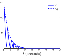
(a)

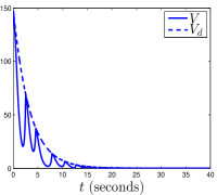
(b)

Figure 1: Instantaneous communication and no disturbance: evolution of $V_{d}$ and $V$ under the event-triggered design (23) for (a) $\bar{p}=12$ and (b) $\bar{p}=20$.

Figure 1 shows the evolution of $V$ and $V_{d}$ in both cases. As established in Theorem IV.7, the desired convergence rate is guaranteed in each case. In the case of $\bar{p}=12$, it turns out that $\underline{p_{k}}=\bar{p}$ for each $k\in{\mathbb{N}}$. On the other hand, in the case when $\bar{p}=20$, the performance of $V$ with respect to $V_{d}$ plays a more relevant role in determining the transmission times in (23). In fact, in the presented simulation, $\underline{p_{k}}<\bar{p}$ on all transmissions, as depicted in Figure 2(a). Figure 2(b) shows the interpolated plot of the total number of bits transmitted for both cases, $\bar{p}=12$ and $\bar{p}=20$ along with sufficient (Corollary IV.4) and necessary (Proposition III.2) data rate.

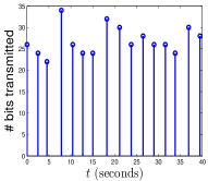
(a)

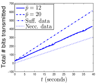
(b)

Figure 2: For the event-triggered implementations in Figure 1, (a) shows the number of bits on each transmission when $\bar{p}=20$ and (b) shows the interpolated plot of the total number of bits transmitted when $\bar{p}=12,20$; along with sufficient (Corollary V.7) and necessary (Proposition III.2) data.

Although in reality the total number of bits transmitted as a function of time is piecewise constant, the interpolated plots enable a more insightful comparison. In the case $\bar{p}=20$, after having transmitted more bits initially than for $\bar{p}=12$, the gap in the cumulative bit counts diminishes eventually. Finally, during the time interval $[0,40]$, the number of transmissions, average inter-transmission time, and minimum inter-transmission time are $18$, $2.2995$ and $0.8585$ (case $\bar{p}=12$) and $16$, $2.63$ and $2.048$ (case $\bar{p}=20$), respectively.

Non-instantaneous communication and non-zero disturbance: we let $\nu=0.01$ and, following (15b) with $\sigma=0.9$, we set $V_{0}=5.3942$, for which we obtain $\Gamma_{1}(1,1)=0.0347$. The actual disturbance signal employed in the simulation is

$$v_{1}(t)=\nu\sin(0.5t),\quad v_{2}(t)=\nu\cos(0.5t).$$

We present a simulation for the case $\bar{p}=20$. We choose $T_{M}=0.8\times\min\{\Gamma_{1}(1,1),T,T^{*}\}=1.1\times 10^{-3}$ and the communication time $\Delta_{k}=r_{k}-t_{k}=T_{M}$ for all $k\in{\mathbb{N}}$ (consequently, note that $R_{k}=T_{k}$ for $k\in{\mathbb{N}}_{0}$).

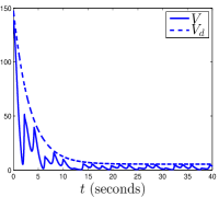
(a)

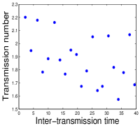
(b)

Figure 3: Non-instantaneous communication and non-zero disturbance: (a) shows the evolution of $V_{d}$ and $V$ and (b) shows the inter-transmission times under the event-triggered design (28) for $\bar{p}=20$.

Figure 3(a) shows the evolution of $V$ and $V_{d}$, which is in accordance with Theorem V.4, while Figure 3(b) shows the inter-transmission times.

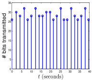
(a)

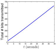
(b)

Figure 4: For the event-triggered implementation shown in Figure 3(a) with $\bar{p}=20$, (a) shows the number of bits on each transmission and (b) shows the interpolated plot of the total number of bits transmitted.

Figure 4 displays the evolution of the number of bits transmitted. During the time interval $[0,40]$, the number of transmissions is $22$, with average and minimum inter-transmission intervals of $1.8182$ and $1.5739$, respectively.

Non-instantaneous communication and no disturbance: we let $\nu=V_{0}=0$, $\bar{p}=20$ and $T_{M}=1.1\times 10^{-3}$. The values of $\Gamma_{1}(1,1)$ and $T$ are as in the case of instantaneous communication with no disturbance. We choose the communication time as $\Delta_{k}=r_{k}-t_{k}=T_{M}$ for all $k\in{\mathbb{N}}$. To illustrate Corollary V.7, we compare the results of two simulations: in “Sim1” we choose $p_{k}=\underline{p_{k}}$ for all $k\in{\mathbb{N}}$ while in “Sim2” we choose $p_{k}=\bar{p}$ for $k\in\{1,2,3,4\}$ and $p_{k}=\underline{p_{k}}$ for all $k\in[5,\infty)\cap{\mathbb{N}}$. Figure 5(a) shows the number of bits on each transmission for “Sim2” while Figure 5(b) compares the interpolated total number of bits transmitted in “Sim1” and “Sim2”. Notice that until $5^{\text{th}}$ transmission time of “Sim2”, the cumulative bit count for “Sim2” exceeds that of “Sim1” but the gap is immediately closed at that time and thereafter remains slightly lower than that of “Sim1”. This demonstrates the ability of the event-trigger design to transmit fewer bits if more bits than prescribed were transmitted in the past. We also see that the data rate, as interpreted in Corollary V.7, remains approximately fixed irrespective of the past history of transmitted bit count as long as the constraints of Theorem V.4 are respected. We have not observed a similar behavior in the scenario with disturbance.

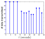
(a)

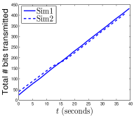
(b)

Figure 5: For non-instantaneous communication without disturbance and $\bar{p}=20$, (a) shows the number of bits on each transmission for “Sim2” (b) shows a comparison of the interpolated total number of bits transmitted in “Sim1,2”.

VII Conclusions

We have studied the problem of exponential practical stabilization of linear-time invariant systems, in the presence of disturbance, and under bounded communication bit rates. Our event-triggered design opportunistically determines the times for communication as well as the numbers of bits to be transmitted at each time. Given a uniform bound on the norm of the disturbance and a prescribed rate of convergence, the control strategy proposed here asymptotically confines the plant to a compact set, guarantees a uniform positive lower bound on inter-transmission and inter-reception communication times, and ensures that the number of bits transmitted at each transmission is uniformly upper bounded. These guarantees are valid for instantaneous transmissions with finite precision data as well as for non-instantaneous transmissions with bounded communication rate. The combination of elements from event-triggered control and information theory has also enabled us to guarantee an arbitrarily prescribed convergence rate (something not typically ensured in the information-theoretic approach) and characterize necessary and sufficient conditions on the number of bits required for stabilization under opportunistic transmissions (an issue mostly overlooked in event-triggered control).

Among the limitations of our work are the assumption of known communication delays and the related requirement of synchronized updates by the encoder and the decoder for maintaining a synchronized quantization domain. Additionally, the coding scheme we have used, though simple, is conservative and introduces a gap between the necessary and sufficient data rates. Future work will also explore better characterization of data rates under disturbances, the characterization of the gain in performance of dynamic controllers over static ones, the extension of the results to stochastic time-varying communication channels, and, more generally, the understanding of the trade-offs between system performance and timeliness and size of transmissions.

Pavankumar Tallapragada received the B.E. degree in Instrumentation Engineering from SGGS Institute of Engineering $\&$ Technology, Nanded, India in 2005, M.Sc. (Engg.) degree in Instrumentation from the Indian Institute of Science, Bangalore, India in 2007 and the Ph.D. degree in Mechanical Engineering from the University of Maryland, College Park in 2013. He is currently a Postdoctoral Scholar in the Department of Mechanical and Aerospace Engineering at the University of California, San Diego. His research interests include event-triggered control, networked control systems, distributed control and transportation and traffic systems.

Jorge Cortés received the Licenciatura degree in mathematics from Universidad de Zaragoza, Zaragoza, Spain, in 1997, and the Ph.D. degree in engineering mathematics from Universidad Carlos III de Madrid, Madrid, Spain, in 2001. He held post-doctoral positions with the University of Twente, Twente, The Netherlands, and the University of Illinois at Urbana-Champaign, Urbana, IL, USA. He was an Assistant Professor with the Department of Applied Mathematics and Statistics, University of California, Santa Cruz, CA, USA, from 2004 to 2007. He is currently a Professor in the Department of Mechanical and Aerospace Engineering, University of California, San Diego, CA, USA. He is the author of Geometric, Control and Numerical Aspects of Nonholonomic Systems (Springer-Verlag, 2002) and co-author (together with F. Bullo and S. Martínez) of Distributed Control of Robotic Networks (Princeton University Press, 2009). He is an IEEE Fellow and an IEEE Control Systems Society Distinguished Lecturer. His current research interests include distributed control, networked games, power networks, distributed optimization, spatial estimation, and geometric mechanics.

References

- [1] K. D. Kim and P. R. Kumar, “Cyber–physical systems: A perspective at the centennial,” Proceedings of the IEEE, vol. 100, no. Special Centennial Issue, pp. 1287–1308, 2012.
- [2] J. Sztipanovits, X. Koutsoukos, G. Karsai, N. Kottenstette, P. Antsaklis, V. Gupta, B. Goodwine, J. Baras, and S. Wang, “Toward a science of cyber–physical system integration,” Proceedings of the IEEE, vol. 100, no. 1, pp. 29–44, 2012.
- [3] G. N. Nair, F. Fagnani, S. Zampieri, and R. J. Evans, “Feedback control under data rate constraints: an overview,” Proceedings of the IEEE, vol. 95, no. 1, pp. 108–137, 2007.
- [4] M. Franceschetti and P. Minero, “Elements of information theory for networked control systems,” in Information and Control in Networks, G. Como, B. Bernhardsson, and A. Rantzer, Eds. New York: Springer, 2014, vol. 450, pp. 3–37.
- [5] G. N. Nair and R. J. Evans, “Stabilization with data-rate-limited feedback: Tightest attainable bounds,” Systems & Control Letters, vol. 41, no. 1, pp. 49–56, 2000.
- [6] ——, “Stabilizability of stochastic linear systems with finite feedback data rates,” SIAM Journal on Control and Optimization, vol. 43, no. 2, pp. 413–436, 2004.
- [7] S. Tatikonda and S. Mitter, “Control under communication constraints,” IEEE Transactions on Automatic Control, vol. 49, no. 7, pp. 1056–1068, 2004.
- [8] N. Martins, M. Dahleh, and N. Elia, “Feedback stabilization of uncertain systems in the presence of a direct link,” IEEE Transactions on Automatic Control, vol. 51, no. 3, pp. 438–447, 2006.
- [9] P. Minero, M. Franceschetti, S. Dey, and G. N. Nair, “Data rate theorem for stabilization over time-varying feedback channels,” IEEE Transactions on Automatic Control, vol. 54, no. 2, pp. 243–255, 2009.
- [10] P. Minero, L. Coviello, and M. Franceschetti, “Stabilization over Markov feedback channels: the general case,” IEEE Transactions on Automatic Control, vol. 58, no. 2, pp. 349–362, 2013.
- [11] L. Keyong and J. Baillieul, “Robust quantization for digital finite communication bandwidth (dfcb) control,” IEEE Transactions on Automatic Control, vol. 49, no. 9, pp. 1573–1584, 2004.
- [12] ——, “Robust and efficient quantization and coding for control of multidimensional linear systems under data rate constraints,” International Journal on Robust and Nonlinear Control, vol. 17, pp. 898–920, 2007.
- [13] C. D. Persis, “-bit stabilization of -dimensional nonlinear systems in feedforward form,” IEEE Transactions on Automatic Control, vol. 50, no. 3, pp. 299–311, 2005.
- [14] D. Liberzon, “Finite data-rate feedback stabilization of switched and hybrid linear systems,” Automatica, vol. 50, no. 2, pp. 409–420, 2014.
- [15] P. Tabuada, “Event-triggered real-time scheduling of stabilizing control tasks,” IEEE Transactions on Automatic Control, vol. 52, no. 9, pp. 1680–1685, 2007.
- [16] X. Wang and M. D. Lemmon, “Event-triggering in distributed networked control systems,” IEEE Transactions on Automatic Control, vol. 56, no. 3, pp. 586–601, 2011.
- [17] W. P. M. H. Heemels, K. H. Johansson, and P. Tabuada, “An introduction to event-triggered and self-triggered control,” in IEEE Conf. on Decision and Control, Maui, HI, 2012, pp. 3270–3285.
- [18] P. Tallapragada and N. Chopra, “On co-design of event trigger and quantizer for emulation based control,” in American Control Conference, Montreal, Canada, June 2012, pp. 3772–3777.
- [19] E. Garcia and P. J. Antsaklis, “Model-based event-triggered control for systems with quantization and time-varying network delays,” IEEE Transactions on Automatic Control, vol. 58, no. 2, pp. 422–434, 2013.
- [20] D. Lehmann and J. Lunze, “Event-based control using quantized state information,” in IFAC Workshop on Distributed Estimation and Control in Networked Systems, Annecy, France, Sept. 2010, pp. 1–6.
- [21] L. Li, X. Wang, and M. D. Lemmon, “Stabilizing bit-rates in quantized event triggered control systems,” in International Conference on Hybrid Systems: Computation and Control, Beijing, China, 2012, pp. 245–254.
- [22] ——, “Stabilizing bit-rate of disturbed event triggered control systems,” in Proceedings of the 4th IFAC Conference on Analysis and Design of Hybrid Systems, Eindhoven, Netherlands, June 2012, pp. 70–75.
- [23] L. Li, B. Hu, and M. D. Lemmon, “Resilient event triggered systems with limited communication,” in IEEE Conf. on Decision and Control, Maui, HI, Dec. 2012, pp. 6577–6582.
- [24] Y. Sun and X. Wang, “Stabilizing bit-rates in networked control systems with decentralized event-triggered communication,” Discrete Event Dynamic Systems, vol. 24, no. 2, pp. 219–245, 2014.
- [25] D. Liberzon, Switching in Systems and Control, ser. Systems & Control: Foundations & Applications. Birkhäuser, 2003.
- [26] H. K. Khalil, Nonlinear Systems, 3rd ed. Prentice Hall, 2002.