Dynamical Widom–Rowlinson model and its mesoscopic limit

Abstract

We consider the non-equilibrium dynamics for the Widom–Rowlinson model (without hard-core) in the continuum. The Lebowitz–Penrose-type scaling of the dynamics is studied and the system of the corresponding kinetic equations is derived. In the space-homogeneous case, the equilibrium points of this system are described. Their structure corresponds to the dynamical phase transition in the model. The bifurcation of the system is shown.

1 Introduction

Critical behavior of complex systems in the continuum is one of the central problems in statistical physics. For systems in $\mathbb{R}^{d}$, $d>1$, consisting of particles of the same type there is, up to our knowledge, only one rigorous mathematical analysis of this problem, the so-called LMP (Lebowitz–Mazel–Presutti) models with Kac potentials, see [23, Chapter 10] and the references therein. The case of particles of different types has been more extensively studied. The simplest model was proposed by Widom and Rowlinson [26] for a potential with hard-core. In this model, there is an interaction only between particles of different types. For large activity, the existence of phase transition for the model in [26] was shown by Ruelle [24]. A natural modification of this model for the case of three or more different particle types is the Potts model in the continuum. Within this context, Lebowitz and Lieb [22] extended Ruelle’s result to the multi-types case and soft-core potentials. For a large class of potentials (with or without soft-core), Georgii and Häggström [13] established the phase transition. Further activity in this area concerns a mean-field theory for the Potts model in the continuum and, in particular, for the Widom–Rowlinson model, without hard-core, see [14] for the most general case (that is, two or more different types) and [4, 5] (for three or more different types).

All these works deal with Gibbs equilibrium states of continuous particle systems. Another approach to study Gibbs measures goes back to Glauber and Dobrushin and it consists in the analysis of the stochastic dynamics associated with these measures. In the continuous case, an analogue of the Glauber dynamics is a spatial birth-and-death process whose intensities imply the invariance of the dynamics with respect to a proper Gibbs measure (the so-called detailed balance conditions). For continuous particle systems of only one type, the corresponding non-equilibrium dynamics was recently intensively studied, see e.g. [9, 11] and the references therein. In this work we consider the corresponding Glauber-type dynamics in the continuum, but for two different particle types. Here we use the statistical Markov evolution rather than the dynamics in the sense of trajectories. In other words, we study the dynamics in terms of states. This can be done using the language of correlation functions corresponding to the states or the language of the corresponding generating functionals.

We construct this dynamics for the Widom–Rowlinson model and study its mesoscopic behavior under the so-called Lebowitz–Penrose scaling (see [23] and the references therein). For this purpose, we exploit a technique based on the Ovsjannikov theorem, see e.g. [11] and the references therein. This allows us to derive rigorously the system of kinetic equations for the dynamics, which critical behavior reflects the phase transition phenomenon in the original microscopic dynamics. This scheme to derive the kinetic equations for Markov evolutions in the continuum was proposed in [7] and goes back to an approach well-known for the Hamiltonian dynamics, see [25]. Another approach is based on minimizing some energy functionals, see e.g. [2, 3].

In Section 2 we briefly recall some notions of the analysis on one- and two-types configuration spaces. A more detailed explanation can be found in e.g. [1, 17] and [6, 12], respectively. We introduce and study a generalization of generating functionals for two-types spaces as well. In Section 3 we consider the dynamical Widom–Rowlinson model. We prove that the corresponding time evolution in terms of entire generating functionals exist in a scale of Banach spaces, for a finite time interval (Theorem 3.5). Section 4 is devoted to the mesoscopic scaling in the Lebowitz–Penrose sense. We prove that the rescaled evolution of entire generating functionals converges strongly to the limiting time evolution (Theorem 4.5). The latter preserves exponential functionals (Theorem 4.6), which corresponds to the propagation of the chaos principle for correlation functions, cf. e.g. [10]. This allows to derive a system of kinetic equations (4.13), which are non-linear and non-local (they include convolutions of functions on $\mathbb{R}^{d}$, cf. e.g. [8]). We also prove the existence and uniqueness of the solutions to the aforementioned system of equations (Theorem 4.7). In Section 5 we consider the same system but in the space-homogeneous case. Even this simplest case reflects the dynamical phase transition, which is expected to occur in the original non-equilibrium dynamics. Namely, in Theorem 5.2 we prove that there is a critical value below of which the system of kinetic equations will have a unique stable equilibrium point. For higher values, the system will have three equilibrium points: two of them are stable (they correspond to the pure phases of the reversible Gibbs measure) and the third one is unstable (it corresponds to the symmetric mixed phase). It is worth noting that at the critical point the system has a unique mixed equilibrium point (saddle-node). Therefore, there is a bifurcation in the system of the kinetic equations corresponding to the dynamical Widom–Rowlinson model without hard-core. We note that the existence of such a critical value for the original (equilibrium) model was an open problem, see e.g. [13, Remark 1.3].

2 General Framework

This section begins by briefly recalling the concepts and results of combinatorial harmonic analysis on one- and two-types configuration spaces needed throughout this work. For a detailed explanation see e.g. [1, 6, 12, 17] and the references cited therein.

2.1 One-component configuration spaces

The configuration space $\Gamma:=\Gamma_{\mathbb{R}}$ over $\mathbb{R}^{d}$, $d\in\mathbb{N}$, is defined as the set of all locally finite subsets (configurations) of $\mathbb{R}^{d}$,

$$\Gamma:=\left\{\gamma\subset\mathbb{R}^{d}:|\gamma\cap\Lambda|<\infty\hbox{ for every compact }\Lambda\subset\mathbb{R}^{d}\right\},$$

where $\left|\cdot\right|$ denotes the cardinality of a set. We will identify a configuration $\gamma\in\Gamma$ with the non-negative Radon measure $\sum_{x\in\gamma}\delta_{x}$ on the Borel $\sigma$-algebra $\mathcal{B}(\mathbb{R}^{d})$, where $\delta_{x}$ is the Dirac measure with mass $1$ at $x$ and $\sum_{x\in\emptyset}\delta_{x}:=0$. This identification allows to endow $\Gamma$ with the vague topology and the corresponding Borel $\sigma$-algebra $\mathcal{B}(\Gamma)$.

Let $\rho>0$ be a locally integrable function on $\mathbb{R}^{d}$. The Poisson measure $\pi_{\sigma}$ with intensity the Radon measure

$$d\sigma(x)=\rho(x)dx$$

is defined as the probability measure on $(\Gamma,\mathcal{B}(\Gamma))$ with Laplace transform given by

$$\int_{\Gamma}d\pi_{\sigma}(\gamma)\,\exp\biggl{(}\sum_{x\in\gamma}\varphi(x)\biggr{)}=\exp\biggl{(}\int_{\mathbb{R}^{d}}dx\,\rho(x)\left(e^{\varphi(x)}-1\right)\biggr{)}$$

for all smooth functions $\varphi$ on $\mathbb{R}^{d}$ with compact support. For the case $\rho\equiv 1$, we will omit the index $\pi:=\pi_{dx}$.

For any $n\in\mathbb{N}_{0}:=\mathbb{N}\cup\{0\}$, let

$$\Gamma^{(n)}:=\{\gamma\in\Gamma:|\gamma|=n\},\ n\in\mathbb{N},\quad\Gamma^{(0)}:=\{\emptyset\}.$$

Clearly, each $\Gamma^{(n)}$, $n\in\mathbb{N}$, can be identified with the symmetrization of the set $\{(x_{1},...,x_{n})\in(\mathbb{R}^{d})^{n}:x_{i}\not=x_{j}\hbox{ if }i\not=j\}$ under the permutation group over $\{1,...,n\}$, which induces a natural (metrizable) topology on $\Gamma^{(n)}$ and the corresponding Borel $\sigma$-algebra $\mathcal{B}(\Gamma^{(n)})$. Moreover, for the product measure $\sigma^{\otimes n}$ fixed on $(\mathbb{R}^{d})^{n}$, this identification yields a measure $\sigma^{(n)}$ on $(\Gamma^{(n)},\mathcal{B}(\Gamma^{(n)}))$. This leads to the space of finite configurations

$$\Gamma_{0}:=\bigsqcup_{n=0}^{\infty}\Gamma^{(n)}$$

endowed with the topology of disjoint union of topological spaces and the corresponding Borel $\sigma$-algebra $\mathcal{B}(\Gamma_{0})$, and to the so-called Lebesgue–Poisson measure on $(\Gamma_{0},\mathcal{B}(\Gamma_{0}))$,

$$\lambda_{\sigma}:=\sum_{n=0}^{\infty}\frac{1}{n!}\sigma^{(n)},\quad\sigma^{(0)}(\{\emptyset\}):=1.$$

We set $\lambda:=\lambda_{dx}$.

2.2 Two-component configuration spaces

The previous definitions can be naturally extended to $n$-component configuration spaces. Having in mind our goals, we just present the extension for $n=2$.

Given two copies of the space $\Gamma$, denoted by $\Gamma^{+}$ and $\Gamma^{-}$, let

$$\Gamma^{2}:=\left\{(\gamma^{+},\gamma^{-})\in\Gamma^{+}\times\Gamma^{-}:\gamma^{+}\cap\gamma^{-}=\emptyset\right\}.$$

Similarly, given two copies of the space $\Gamma_{0}$, denoted by $\Gamma_{0}^{+}$ and $\Gamma_{0}^{-}$, we consider the space

$$\Gamma^{2}_{0}:=\left\{(\eta^{+},\eta^{-})\in\Gamma_{0}^{+}\times\Gamma_{0}^{-}:\eta^{+}\cap\eta^{-}=\emptyset\right\}.$$

We endow $\Gamma^{2}$ and $\Gamma_{0}^{2}$ with the topology induced by the product of the topological spaces $\Gamma^{+}\times\Gamma^{-}$ and $\Gamma_{0}^{+}\times\Gamma_{0}^{-}$, respectively, and with the corresponding Borel $\sigma$-algebras, denoted by $\mathcal{B}(\Gamma^{2})$ and $\mathcal{B}(\Gamma^{2}_{0})$.

We consider the space $B_{\mathrm{ls}}(\Gamma_{0}^{2})$ of all complex-valued $\mathcal{B}(\Gamma^{2}_{0})$-measurable functions $G$ with local support, i.e., $G\!\!\upharpoonright_{\Gamma_{0}^{2}\backslash\left(\Gamma_{\Lambda}^{+}\times\Gamma_{\Lambda}^{-}\right)}\equiv 0$ for some bounded set $\Lambda\in\mathcal{B}(\mathbb{R}^{d})$, where $\Gamma_{\Lambda}^{\pm}:=\{\eta\in\Gamma^{\pm}:\eta\subset\Lambda\}$. Given a $G\in B_{\mathrm{ls}}(\Gamma_{0}^{2})$, the ${\mathrm{K}}$-transform of $G$ is the mapping ${\mathrm{K}}G:\Gamma^{2}\to\mathbb{C}$ defined at each $(\gamma^{+},\gamma^{-})\in\Gamma^{2}$ by

$$({\mathrm{K}}G)(\gamma^{+},\gamma^{-}):=\sum_{\begin{subarray}{c}\eta^{+}\subset\gamma^{+}\\ |\eta^{+}|<\infty\end{subarray}}\sum_{\begin{subarray}{c}\eta^{-}\subset\gamma^{-}\\ |\eta^{-}|<\infty\end{subarray}}G(\eta^{+},\eta^{-}).$$ (2.1)

Note that for every $G\in B_{\mathrm{ls}}(\Gamma_{0}^{2})$ the sum in (2.1) has only a finite number of summands different from zero and thus ${\mathrm{K}}G$ is a well-defined function on $\Gamma^{2}$. Moreover, ${\mathrm{K}}:B_{\mathrm{ls}}(\Gamma_{0}^{2})\to{\mathrm{K}}(B_{\mathrm{ls}}(\Gamma_{0}^{2}))$ is a positivity preserving linear isomorphism whose inverse mapping is defined by

$$\left({\mathrm{K}}^{-1}F\right)(\eta^{+},\eta^{-}):=\sum_{\xi^{+}\subset\eta^{+}}\sum_{\xi^{-}\subset\eta^{-}}(-1)^{|\eta^{+}\backslash\xi^{+}|+|\eta^{-}\backslash\xi^{-}|}F(\xi^{+},\xi^{-}),\quad(\eta^{+},\eta^{-})\in\Gamma_{0}^{2}.$$

The ${\mathrm{K}}$-transform might be extended pointwisely to a wider class of functions. Among them we will distinguish the so-called Lebesgue–Poisson exponentials $e_{\lambda}(f^{+},f^{-})$ defined for complex-valued $\mathcal{B}(\mathbb{R}^{d})$-measurable functions $f^{+},f^{-}$ by

$$e_{\lambda}(f^{+},f^{-};\eta^{+},\eta^{-}):=e_{\lambda}(f^{+},\eta^{+})e_{\lambda}(f^{-},\eta^{-}),\quad(\eta^{+},\eta^{-})\in\Gamma_{0}^{2},$$ (2.2)

where

$$e_{\lambda}(f^{\pm},\eta^{\pm}):=\prod_{x\in\eta^{\pm}}f^{\pm}(x),\ \eta^{\pm}\in\Gamma^{\pm}_{0}\!\setminus\!\{\emptyset\},\quad e_{\lambda}(f^{\pm},\emptyset):=1.$$

Indeed, for any $f^{+},f^{-}$ described as before, having in addition compact support, for all $(\gamma^{+},\gamma^{-})\in\Gamma^{2}$

$$\left({\mathrm{K}}e_{\lambda}(f^{+},f^{-})\right)(\gamma^{+},\gamma^{-})=\prod_{x\in\gamma^{+}}\bigl{(}1+f^{+}(x)\bigr{)}\prod_{y\in\gamma^{-}}\bigl{(}1+f^{-}(y)\bigr{)}.$$ (2.3)

The special role of functions (2.2) is partially due to the fact that the right-hand side of (2.3) coincides with the integrand functions of generating functionals (Subsection 2.3 below).

Let now $\mathcal{M}_{\mathrm{fm}}^{1}(\Gamma^{2})$ be the set of all probability measures $\mu$ on $(\Gamma^{2},\mathcal{B}(\Gamma^{2}))$ with finite local moments of all orders, i.e., for all $n\in\mathbb{N}$ and all bounded sets $\Lambda\in\mathcal{B}(\mathbb{R}^{d})$

$$\int_{\Gamma^{2}}d\mu(\gamma^{+},\gamma^{-})\,|\gamma^{+}\cap\Lambda|^{n}|\gamma^{-}\cap\Lambda|^{n}<\infty,$$

and let $B_{\mathrm{bs}}(\Gamma_{0}^{2})$ be the set of all bounded functions $G\in B_{\mathrm{ls}}(\Gamma_{0}^{2})$ such that $G\!\!\upharpoonright_{\Gamma_{0}^{2}\backslash\left(\bigsqcup_{n=0}^{N^{+}}\Gamma_{\Lambda^{+}}^{(n)}\times\bigsqcup_{n=0}^{N^{-}}\Gamma_{\Lambda^{-}}^{(n)}\right)}\equiv 0$ for some $N^{+},N^{-}\in\mathbb{N}_{0}$ and for some bounded Borel sets $\Lambda^{+},\Lambda^{-}\subset\mathbb{R}^{d}$. Here, for $k\in\mathbb{N}_{0}$ and for bounded sets $\Lambda^{\pm}\in\mathcal{B}(\mathbb{R}^{d})$, $\Gamma_{\Lambda^{\pm}}^{(k)}:=\{\eta\in\Gamma^{\pm}_{\Lambda^{\pm}}:|\eta|=k\}$. Given a $\mu\in\mathcal{M}_{\mathrm{fm}}^{1}(\Gamma^{2})$, the so-called correlation measure $\rho_{\mu}$ corresponding to $\mu$ is a measure on $(\Gamma_{0}^{2},\mathcal{B}(\Gamma_{0}^{2}))$ defined for all $G\in B_{\mathrm{bs}}(\Gamma_{0}^{2})$ by

$$\int_{\Gamma_{0}^{2}}d\rho_{\mu}(\eta^{+},\eta^{-})\,G(\eta^{+},\eta^{-})=\int_{\Gamma^{2}}d\mu(\gamma^{+},\gamma^{-})\,\left({\mathrm{K}}G\right)(\gamma^{+},\gamma^{-}).$$ (2.4)

Note that under these assumptions ${\mathrm{K}}\left|G\right|$ is $\mu$-integrable, and thus (2.4) is well-defined. In terms of correlation measures, this shows, in particular, that $B_{\mathrm{bs}}(\Gamma_{0}^{2})\subset L^{1}(\Gamma_{0}^{2},\rho_{\mu})$. Actually, $B_{\mathrm{bs}}(\Gamma_{0}^{2})$ is dense in $L^{1}(\Gamma_{0}^{2},\rho_{\mu})$. Moreover, still by (2.4), on $B_{\mathrm{bs}}(\Gamma_{0}^{2})$ the inequality $\|{\mathrm{K}}G\|_{L^{1}(\Gamma^{2},\mu)}\leq\|G\|_{L^{1}(\Gamma_{0}^{2},\rho_{\mu})}$ holds, allowing an extension of the ${\mathrm{K}}$-transform to a bounded operator ${\mathrm{K}}:L^{1}(\Gamma_{0}^{2},\rho_{\mu})\to L^{1}(\Gamma^{2},\mu)$ in such a way that equality (2.4) still holds for any $G\in L^{1}(\Gamma_{0}^{2},\rho_{\mu})$. For the extended operator, the explicit form (2.1) still holds, now $\mu$-a.e. In particular, for functions $f^{+},f^{-}$ such that $e_{\lambda}(f^{+},f^{-})\in L^{1}(\Gamma_{0}^{2},\rho_{\mu})$ equality (2.3) still holds, but only for $\mu$-a.a. $(\gamma^{+},\gamma^{-})\in\Gamma^{2}$.

Let us now consider two measures on $\mathbb{R}^{d}$, in general different, $d\sigma^{\pm}=\rho^{\pm}dx$, both defined as above. The Lebesgue–Poisson product measure $\lambda^{2}_{\sigma^{+},\sigma^{-}}:=\lambda_{\sigma^{+}}\otimes\lambda_{\sigma^{-}}$ on $(\Gamma_{0}^{2},\mathcal{B}(\Gamma_{0}^{2}))$ is the correlation measure corresponding to the Poisson product measure $\pi^{2}_{\sigma^{+},\sigma^{-}}:=\pi_{\sigma^{+}}\otimes\pi_{\sigma^{-}}$ on $(\Gamma^{2},\mathcal{B}(\Gamma^{2}))$. Observe that a priori $\lambda^{2}_{\sigma^{+},\sigma^{-}}$ is a measure defined on $(\Gamma_{0}\times\Gamma_{0},\mathcal{B}(\Gamma_{0})\otimes\mathcal{B}(\Gamma_{0}))$ and $\pi^{2}_{\sigma^{+},\sigma^{-}}$ is a measure defined on $(\Gamma\times\Gamma,\mathcal{B}(\Gamma)\otimes\mathcal{B}(\Gamma))$. It can actually be shown that $\Gamma_{0}^{2}=(\Gamma_{0}\times\Gamma_{0})\setminus\{(\eta,\xi):\eta\cap\xi\not=\emptyset\}$ has full $\lambda^{2}_{\sigma^{+},\sigma^{-}}$-measure and $\Gamma^{2}=(\Gamma\times\Gamma)\setminus\{(\gamma,\gamma^{\prime}):\gamma\cap\gamma^{\prime}\not=\emptyset\}$ has full $\pi^{2}_{\sigma^{+},\sigma^{-}}$-measure, cf. [6, 21].

It can also be shown that $e_{\lambda}(f^{+},f^{-})\in L^{p}(\Gamma_{0}^{2},\lambda^{2}_{\sigma^{+},\sigma^{-}})$ whenever $f^{\pm}\in L^{p}(\mathbb{R}^{d},\sigma^{\pm})$ for some $p\geq 1$, and, moreover,

$$\|e_{\lambda}(f^{+},f^{-})\|^{p}_{L^{p}(\Gamma_{0}^{2},\lambda^{2}_{\sigma^{+},\sigma^{-}})}=\exp(\|f^{+}\|^{p}_{L^{p}(\mathbb{R}^{d},\sigma^{+})}+\|f^{-}\|^{p}_{L^{p}(\mathbb{R}^{d},\sigma^{-})}).$$

In particular, for $p=1$, one additionally has, for all $f^{\pm}\in L^{1}(\mathbb{R}^{d},\sigma^{\pm})$,

$$\int_{\Gamma_{0}^{2}}d\lambda^{2}_{\sigma^{+},\sigma^{-}}(\eta^{+},\eta^{-})\,e_{\lambda}(f^{+},f^{-};\eta^{+},\eta^{-})\\ =\exp\biggl{(}\int_{\mathbb{R}^{d}}dx\left(\rho^{+}(x)f^{+}(x)+\rho^{-}(x)f^{-}(x)\right)\biggr{)}.$$ (2.5)

In the sequel we set

$$\lambda^{2}:=\lambda^{2}_{dx,dx},\qquad\pi^{2}:=\pi^{2}_{dx,dx}.$$

2.3 Bogoliubov generating functionals

The notion of Bogoliubov generating functional corresponding to a probability measure on $(\Gamma,\mathcal{B}(\Gamma))$ [19] naturally extends to probability measures defined on a multicomponent space $(\Gamma^{n},\mathcal{B}(\Gamma^{n}))$. For simplicity, we just present the extension for $n=2$. Of course, a similar procedure is used for $n>2$, but with a more cumbersome notation.

Definition 2.1.

Given a probability measure $\mu$ on $(\Gamma^{2},\mathcal{B}(\Gamma^{2}))$, the Bogoliubov generating functional (shortly GF) $B_{\mu}$ corresponding to $\mu$ is the functional defined at each pair $\theta^{+}$, $\theta^{-}$ of complex-valued $\mathcal{B}(\mathbb{R}^{d})$-measurable functions by

$$B_{\mu}(\theta^{+},\theta^{-}):=\int_{\Gamma^{2}}d\mu(\gamma^{+},\gamma^{-})\,\prod_{x\in\gamma^{+}}\bigl{(}1+\theta^{+}(x)\bigr{)}\prod_{y\in\gamma^{-}}\bigl{(}1+\theta^{-}(y)\bigr{)},$$

provided the right-hand side exists.

Clearly, for an arbitrary probability measure $\mu$, $B_{\mu}$ is always defined at least at the pair $(0,0)$. However, the whole domain of $B_{\mu}$ depends on properties of the underlying measure $\mu$. For instance, probability measures $\mu$ for which the GF is well-defined on multiples of indicator functions ${1\!\!1}_{\Lambda}$ of bounded Borel sets $\Lambda$, necessarily have finite local exponential moments, i.e.,

$$\int_{\Gamma^{2}}d\mu(\gamma^{+},\gamma^{-})\,e^{\alpha(|\gamma^{+}\cap\Lambda|+|\gamma^{-}\cap\Lambda|)}<\infty,\quad\mathrm{for\,\,all}\,\,\alpha>0.$$ (2.6)

The converse is also true. In fact, for all $\alpha>0$ and for all $\Lambda$ described as before we have that the left-hand side of (2.6) is equal to

$$\int_{\Gamma^{2}}d\mu(\gamma^{+},\gamma^{-})\,\prod_{x\in\gamma^{+}\cup\gamma^{-}}e^{\alpha{1\!\!1}_{\Lambda}(x)}\\ =B_{\mu}\bigl{(}(e^{\alpha}-1){1\!\!1}_{\Lambda},(e^{\alpha}-1){1\!\!1}_{\Lambda}\bigr{)}<\infty.$$

According to the previous subsection, this implies that to such a measure $\mu$ one may associate the correlation measure $\rho_{\mu}$, leading to a description of the functional $B_{\mu}$ in terms of the measure $\rho_{\mu}$:

$$B_{\mu}(\theta^{+},\theta^{-}) =\int_{\Gamma^{2}}d\mu(\gamma^{+},\gamma^{-})\,\left({\mathrm{K}}e_{\lambda}(\theta^{+},\theta^{-})\right)(\gamma^{+}\,\gamma^{-})$$

$$=\int_{\Gamma_{0}^{2}}d\rho_{\mu}(\eta^{+},\eta^{-})\,e_{\lambda}(\theta^{+},\theta^{-};\eta^{+},\eta^{-}),$$

or in terms of the so-called correlation function

$$k_{\mu}:=\dfrac{d\rho_{\mu}}{d\lambda^{2}}$$

corresponding to the measure $\mu$, provided $\rho_{\mu}$ is absolutely continuous with respect to the product measure $\lambda^{2}$:

$$B_{\mu}(\theta^{+},\theta^{-})=\int_{\Gamma_{0}^{2}}d\lambda^{2}(\eta^{+},\eta^{-})\,e_{\lambda}(\theta^{+},\theta^{-};\eta^{+},\eta^{-})k_{\mu}(\eta^{+},\eta^{-}).$$ (2.7)

Throughout this work we will consider GF which are entire on the whole $L^{1}(\mathbb{R}^{d},dx)\times L^{1}(\mathbb{R}^{d},dx)$ space with the norm

$$\|(\theta^{+},\theta^{-})\|_{L^{1}\times L^{1}}=\lvert\!\!\lvert\theta^{+}\rvert\!\!\rvert_{1}+\lvert\!\!\lvert\theta^{-}\rvert\!\!\rvert_{1}.$$

Here and below we use the notation

$$\lvert\!\!\lvert\theta\rvert\!\!\rvert_{1}:=\|\theta\|_{L^{1}},\qquad\theta\in L^{1}:=L^{1}(\mathbb{R}^{d},dx).$$

We recall that a functional $A:L^{1}\times L^{1}\to\mathbb{C}$ is entire on $L^{1}\times L^{1}$ whenever $A$ is locally bounded and for all $\theta_{0}^{\pm},\theta^{\pm}\in L^{1}$ the mapping

$$\mathbb{C}^{2}\ni(z^{+},z^{-})\mapsto A(\theta_{0}^{+}+z^{+}\theta^{+},\theta_{0}^{-}+z^{-}\theta^{-})\in\mathbb{C}$$

is entire [20], which is equivalent to entireness on $L^{1}$ of $A$ on each component. Thus, at each pair $\theta_{0}^{+},\theta_{0}^{-}\in L^{1}$, every entire functional $A$ on $L^{1}\times L^{1}$ has a representation in terms of its Taylor expansion,

$$A(\theta_{0}^{+}+z^{+}\theta^{+},\theta_{0}^{-}+z^{-}\theta^{-})\\ =\sum_{n,m=0}^{\infty}\frac{(z^{+})^{n}(z^{-})^{m}}{n!m!}d^{(n,m)}A(\theta_{0}^{+},\theta_{0}^{-};\underbrace{\theta^{+},\ldots,\theta^{+}}_{n\ \text{times}},\underbrace{\theta^{-},\ldots,\theta^{-}}_{m\ \text{times}}),$$

$z^{\pm}\in\mathbb{C}$, $\theta^{\pm}\in L^{1}$. Extending the kernel theorem [19, Theorem 5] to the two-component case, each differential $d^{(n,m)}A(\theta_{0}^{+},\theta_{0}^{-};\cdot)$ is then defined by a kernel $\delta^{(n,m)}A(\theta_{0}^{+},\theta_{0}^{-};\cdot)\in L^{\infty}((\mathbb{R}^{d})^{n}\times(\mathbb{R}^{d})^{m})$, which is symmetric in the first $n$ coordinates and in the last $m$ coordinates. More precisely,

$$d^{(n,m)}A(\theta_{0}^{+},\theta_{0}^{-};\theta_{1}^{+},\ldots,\theta_{n}^{+},\theta^{-}_{1},\ldots,\theta^{-}_{m})$$

$$=\frac{\partial^{n+m}}{\partial z_{1}^{+}...\partial z_{n}^{+}\partial z_{1}^{-}...\partial z_{m}^{-}}A\biggl{(}\theta_{0}^{+}+\sum_{i=1}^{n}z_{i}^{+}\theta_{i}^{+},\theta_{0}^{-}+\sum_{j=1}^{m}z_{j}^{-}\theta_{j}^{-}\biggr{)}\biggr{|}_{z_{1}^{+}=...=z_{n}^{+}=z_{1}^{-}=...=z^{-}_{m}=0}$$

$$=\int_{(\mathbb{R}^{d})^{n}\times(\mathbb{R}^{d})^{m}}dx_{1}\ldots dx_{n}dy_{1}\ldots dy_{m}\,$$

$$\qquad\qquad\times\delta^{(n,m)}A(\theta_{0}^{+},\theta_{0}^{-};x_{1},\ldots,x_{n},y_{1},\ldots,y_{m})\prod_{i=1}^{n}\theta_{i}^{+}(x_{i})\prod_{j=1}^{m}\theta_{j}^{-}(y_{j}),$$

for all $\theta_{1}^{+},...,\theta_{n}^{+},\theta^{-}_{1},...,\theta^{-}_{m}\in L^{1}$, $n,m\in\mathbb{N}$. Moreover, the operator norm of the bounded $(n+m)$-linear functional (on $L^{1}\times L^{1}$) $d^{(n,m)}A(\theta_{0}^{+},\theta_{0}^{-};\cdot)$ is equal to $\left\|\delta^{(n,m)}A(\theta_{0}^{+},\theta_{0}^{-};\cdot)\right\|_{L^{\infty}((\mathbb{R}^{d})^{n}\times(\mathbb{R}^{d})^{m})}$ and for all $r>0$ one has

$$\left\|\delta^{(n,m)}{A}(\theta_{0}^{+},\theta_{0}^{-};\cdot)\right\|_{L^{\infty}((\mathbb{R}^{d})^{n}\times(\mathbb{R}^{d})^{m})}\\ \leq n!m!\left(\frac{e}{r}\right)^{n+m}\sup_{\lvert\!\!\lvert\theta^{\pm}\rvert\!\!\rvert_{1}\leq r}|A(\theta_{0}^{+}+\theta^{+},\theta_{0}^{-}+\theta^{-})|.$$

For the cases where either $n=0$ or $m=0$, the entireness property on $L^{1}$ of each pair of functionals $A(\cdot,\theta_{0}^{-})$, $A(\theta_{0}^{+},\cdot)$ implies by a direct application of [19, Theorem 5] that the corresponding differentials are defined by a symmetric kernel $\delta^{n}{A}(\theta_{0}^{+},\theta_{0}^{-};\cdot,\emptyset)\in L^{\infty}((\mathbb{R}^{d})^{n})$, $\delta^{m}{A}(\theta_{0}^{+},\theta_{0}^{-};\emptyset,\cdot)\in L^{\infty}((\mathbb{R}^{d})^{m})$, respectively, and for each $r>0$ one has

$$\left\|\delta A(\theta_{0}^{+},\theta_{0}^{-};\cdot,\emptyset)\right\|_{L^{\infty}}\leq\frac{1}{r}\sup_{\lvert\!\!\lvert\theta^{+}\rvert\!\!\rvert_{1}\leq r}|A(\theta_{0}^{+}+\theta^{+},\theta_{0}^{-})|,$$

$$\left\|\delta A(\theta_{0}^{+},\theta_{0}^{-};\emptyset,\cdot)\right\|_{L^{\infty}}\leq\frac{1}{r}\sup_{\lvert\!\!\lvert\theta^{-}\rvert\!\!\rvert_{1}\leq r}|A(\theta_{0}^{+},\theta_{0}^{-}+\theta^{-})|$$

and, for $n,m\geq 2$,

$$\left\|\delta^{n}{A}(\theta_{0}^{+},\theta_{0}^{-};\cdot,\emptyset)\right\|_{L^{\infty}((\mathbb{R}^{d})^{n})} \leq n!\left(\frac{e}{r}\right)^{n}\sup_{\lvert\!\!\lvert\theta^{+}\rvert\!\!\rvert_{1}\leq r}|A(\theta_{0}^{+}+\theta^{+},\theta_{0}^{+})|,$$

$$\left\|\delta^{m}{A}(\theta_{0}^{+},\theta_{0}^{-};\emptyset,\cdot)\right\|_{L^{\infty}((\mathbb{R}^{d})^{m})} \leq m!\left(\frac{e}{r}\right)^{m}\sup_{\lvert\!\!\lvert\theta^{-}\rvert\!\!\rvert_{1}\leq r}|A(\theta_{0}^{+},\theta_{0}^{-}+\theta^{-})|.$$

All these considerations hold, in particular, for $A$ being an entire GF $B_{\mu}$ on $L^{1}\times L^{1}$ corresponding to some probability measure $\mu$ on $\Gamma^{2}$ which is locally absolutely continuous with respect to $\pi^{2}$, that is, for all disjoint bounded Borel sets $\Lambda^{+},\Lambda^{-}\subset\mathbb{R}^{d}$ the image measure $\mu\circ p_{\Lambda^{+},\Lambda^{-}}^{-1}$ of $\mu$ under the projection $p_{\Lambda^{+},\Lambda^{-}}(\gamma^{+},\gamma^{-}):=(\gamma^{+}\cap\Lambda^{+},\gamma^{-}\cap\Lambda^{-})\in\Gamma_{\Lambda^{+}}\times\Gamma_{\Lambda^{-}}$ is absolutely continuous with respect to the product of image measures $(\pi\circ p_{\Lambda^{+}}^{-1})\times(\pi\circ p_{\Lambda^{-}}^{-1})$, $p_{\Lambda^{\pm}}(\gamma^{\pm}):=\gamma^{\pm}\cap\Lambda^{\pm}$. In this case, the correlation function $k_{\mu}$ exists and it is given for $\lambda^{2}$-a.a. $(\eta^{+},\eta^{-})\in\Gamma_{0}^{2}$ by

$$k_{\mu}(\eta^{+},\eta^{-}) =\delta^{(n,m)}B_{\mu}(0,0;\eta^{+},\eta^{-}),$$

$$k_{\mu}(\eta^{+},\emptyset) =\delta^{n}B_{\mu}(0,0;\eta^{+},\emptyset),$$

$$k_{\mu}(\emptyset,\eta^{-}) =\delta^{m}B_{\mu}(0,0;\emptyset,\eta^{-}),$$

for $|\eta^{+}|=n$, $|\eta^{-}|=m$, $n,m\in\mathbb{N}$ [19, Proposition 9]. As a consequence, similarly to [19, Proposition 11] one finds

$$\delta^{(|\eta^{+}|,|\eta^{-}|)}B_{\mu}(\theta^{+},\theta^{-};\eta^{+},\eta^{-})\\ =\int_{\Gamma_{0}^{2}}d\lambda^{2}(\xi^{+},\xi^{-})\,k_{\mu}(\xi^{+}\cup\eta^{+},\xi^{-}\cup\eta^{-})e_{\lambda}(\theta^{+},\theta^{-};\xi^{+},\xi^{-})$$ (2.8)

for $\lambda^{2}$-a.a. $(\eta^{+},\eta^{-})\in\Gamma_{0}^{2}$, which gives an alternative description of the kernels $\delta^{(n,m)}B_{\mu}(\theta_{0}^{+},\theta_{0}^{-};\cdot)$, $n,m\in\mathbb{N}_{0}$. Moreover, the previous estimates for the norms of the kernels lead to the so-called Ruelle generalized bound [19, Proposition 16], that is, for any $0\leq\varepsilon\leq 1$ and any $r>0$ there is a constant $C\geq 0$ depending on $r$ such that

$$k_{\mu}(\eta^{+},\eta^{-})\leq C\left(\lvert\eta^{+}\rvert!\lvert\eta^{-}\rvert!\right)^{1-\varepsilon}\left(\frac{e}{r}\right)^{\lvert\eta^{+}\rvert+\lvert\eta^{-}\rvert},\quad\lambda^{2}\mathrm{-a.a.\ }(\eta^{+},\eta^{-})\in\Gamma_{0}^{2}.$$

Similarly to the one-component case [19, Proposition 23], the latter motivates for each $\alpha>0$ the definition of the Banach space $\mathcal{E}_{\alpha}$ of all entire functionals $B$ on $L^{1}\times L^{1}$ such that

$$\left\|B\right\|_{\alpha}:=\sup_{\theta^{+},\theta^{-}\in L^{1}}\left(\left|B(\theta^{+},\theta^{-})\right|e^{-\frac{1}{\alpha}\left(\lvert\!\!\lvert\theta^{+}\rvert\!\!\rvert_{1}+\lvert\!\!\lvert\theta^{-}\rvert\!\!\rvert_{1}\right)}\right)<\infty.$$ (2.9)

Observe that this class of Banach spaces has the property that, for each $\alpha_{0}>0$, the family $\{\mathcal{E}_{\alpha}:0<\alpha\leq\alpha_{0}\}$ is a scale of Banach spaces, that is,

$$\mathcal{E}_{\alpha^{\prime\prime}}\subseteq\mathcal{E}_{\alpha^{\prime}},\quad\|\cdot\|_{\alpha^{\prime}}\leq\|\cdot\|_{\alpha^{\prime\prime}}$$

for any pair $\alpha^{\prime}$, $\alpha^{\prime\prime}$ such that $0<\alpha^{\prime}<\alpha^{\prime\prime}\leq\alpha_{0}$.

Of course these considerations hold, more generally, for any entire functional $B$ on $L^{1}\times L^{1}$ of the form

$$B(\theta^{+},\theta^{-})=\int_{\Gamma_{0}^{2}}d\lambda^{2}(\eta^{+},\eta^{-})\,e_{\lambda}(\theta^{+},\theta^{-};\eta^{+},\eta^{-})k(\eta^{+},\eta^{-}),\quad k:\Gamma_{0}^{2}\to\left[0,+\infty\right).$$

3 The Widom–Rowlinson model

The dynamical Widom–Rowlinson model is an example of a birth-and-death model of two different particle types, let us say $+$ and $-$, where, at each random moment of time, $+$ and $-$ particles randomly disappear according to a death rate identically equal to $m>0$, while new $\pm$ particles randomly appear according to a birth rate which only depends on the configuration of the whole $\mp$-system at that time. The influence of the $\pm$-system of particles is none in this process. More precisely, let $\phi:\mathbb{R}^{d}\to\mathbb{R}\cup\{+\infty\}$ be a pair potential, that is, a $\mathcal{B}(\mathbb{R}^{d})$-measurable function such that $\phi(-x)=\phi(x)\in\mathbb{R}$ for all $x\in\mathbb{R}^{d}\setminus\{0\}$, which we will assume to be non-negative and integrable. Given a configuration $(\gamma^{+},\gamma^{-})\in\Gamma^{2}$, the birth rate of a new $+$ particle at a site $x\in\mathbb{R}^{d}\setminus(\gamma^{+}\cup\gamma^{-})$ is given by $\exp(-E(x,\gamma^{-}))$, where $E(x,\gamma^{-})$ is a relative energy of interaction between a particle located at $x$ and the configuration $\gamma^{-}$ defined by

$$E(x,\gamma^{-}):=\sum_{y\in\gamma^{-}}\phi(x-y)\in\left[0,+\infty\right].$$

Similarly, the birth rate of a new $-$ particle at a site $y\in\mathbb{R}^{d}\setminus(\gamma^{+}\cup\gamma^{-})$ is given by $\exp(-E(y,\gamma^{+}))$.

Informally, the behavior of such an infinite particle system is described by a pre-generator

$$(LF)(\gamma^{+},\gamma^{-}):= \,m\sum_{x\in\gamma^{+}}\left(F(\gamma^{+}\setminus x,\gamma^{-})-F(\gamma^{+},\gamma^{-})\right)$$

$$+m\sum_{y\in\gamma^{-}}\left(F(\gamma^{+},\gamma^{-}\setminus y)-F(\gamma^{+},\gamma^{-})\right)$$

$$+z\int_{\mathbb{R}^{d}}dx\,e^{-E(x,\gamma^{-})}\left(F(\gamma^{+}\cup x,\gamma^{-})-F(\gamma^{+},\gamma^{-})\right)$$

$$+z\int_{\mathbb{R}^{d}}dy\,e^{-E(y,\gamma^{+})}\left(F(\gamma^{+},\gamma^{-}\cup y)-F(\gamma^{+},\gamma^{-})\right),$$

where $z>0$ is an activity parameter. Of course, the previous expression will be well-defined under proper conditions on the function $F$ [12].

In applications, properties of the time evolution of an infinite particle system, like the described one, in terms of states, that is, probability measures on $\Gamma^{2}$, are a subject of interest. Informally, such a time evolution is given by the so-called Fokker–Planck equation

$$\frac{d\mu_{t}}{dt}=L^{*}\mu_{t},\quad{\mu_{t}}_{|t=0}=\mu_{0},$$ (3.1)

where $L^{*}$ is the dual operator of $L$. As explained in [12], technically the use of definition (2.4) allows an alternative approach to the study of (3.1) through the corresponding correlation functions $k_{t}:=k_{\mu_{t}}$, $t\geq 0$, provided they exist. This leads to the Cauchy problem

$$\frac{\partial}{\partial t}k_{t}=\widehat{L}^{*}k_{t},\quad{k_{t}}_{|t=0}=k_{0},$$

where $k_{0}$ is the correlation function corresponding to the initial distribution $\mu_{0}$ of the system and $\widehat{L}^{*}$ is the dual operator of $\widehat{L}:={\mathrm{K}}^{-1}L{\mathrm{K}}$ in the sense

$$\int_{\Gamma_{0}^{2}}d\lambda^{2}(\eta^{+},\eta^{-})\,(\widehat{L}G)(\eta^{+},\eta^{-})k(\eta^{+},\eta^{-})\\ =\int_{\Gamma_{0}^{2}}d\lambda^{2}(\eta^{+},\eta^{-})\,G(\eta^{+},\eta^{-})(\widehat{L}^{*}k)(\eta^{+},\eta^{-}).$$ (3.2)

To define $\widehat{L}$ and $\widehat{L}^{*}$ with a full rigor, see [12].

Now we would like to rewrite the dynamics (3.1) in terms of the GF $B_{t}$ corresponding to $\mu_{t}$. Through the representation (2.7), this can be done, informally, by

$$\frac{\partial}{\partial t}B_{t}(\theta^{+},\theta^{-}) =\int_{\Gamma_{0}^{2}}d\lambda^{2}(\eta^{+}\eta^{-})\,e_{\lambda}(\theta^{+},\theta^{-};\eta^{+},\eta^{-})\Bigl{(}\frac{\partial}{\partial t}k_{t}(\eta^{+},\eta^{-})\Bigr{)}$$ (3.3)

$$=\int_{\Gamma_{0}^{2}}d\lambda^{2}(\eta^{+},\eta^{-})\,e_{\lambda}(\theta^{+},\theta^{-};\eta^{+},\eta^{-})(\widehat{L}^{*}k_{t})(\eta^{+},\eta^{-})$$

$$=\int_{\Gamma_{0}^{2}}d\lambda^{2}(\eta^{+},\eta^{-})\,(\widehat{L}e_{\lambda}(\theta^{+},\theta^{-}))(\eta^{+},\eta^{-})k_{t}(\eta^{+},\eta^{-}),$$

for all $\theta^{\pm}\in L^{1}$. In other words, given the operator $\widetilde{L}$ defined at

$$B(\theta^{+},\theta^{-}):=\int_{\Gamma_{0}^{2}}d\lambda^{2}(\eta^{+},\eta^{-})\,e_{\lambda}(\theta^{+},\theta^{-};\eta^{+},\eta^{-})k(\eta^{+},\eta^{-}),$$

for some $k:\Gamma_{0}^{2}\to\left[0,+\infty\right)$, by

$$(\widetilde{L}B)(\theta^{+},\theta^{-}):=\int_{\Gamma_{0}^{2}}d\lambda^{2}(\eta^{+},\eta^{-})\,(\widehat{L}e_{\lambda}(\theta^{+},\theta^{-}))(\eta^{+},\eta^{-})k(\eta^{+},\eta^{-}),$$

one has that the GF $B_{t}$, $t\geq 0$ are a (pointwise) solution to the equation

$$\frac{\partial B_{t}}{\partial t}=\widetilde{L}B_{t}.$$

We will find now an explicit expression for the operator $\widetilde{L}$. The fact that the expression is well-defined will follow from Proposition 3.2 below.

Proposition 3.1.

For all $\theta^{\pm}\in L^{1}$, we have

$$(\widetilde{L}B)(\theta^{+},\theta^{-})$$

$$= -\int_{\mathbb{R}^{d}}dx\,\theta^{+}(x)\bigl{(}m\delta B(\theta^{+},\theta^{-};x,\emptyset)-zB(\theta^{+},\theta^{-}e^{-\phi(x-\cdot)}+e^{-\phi(x-\cdot)}-1)\bigr{)}$$

$$-\int_{\mathbb{R}^{d}}dy\,\theta^{-}(y)\bigl{(}m\delta B(\theta^{+},\theta^{-};\emptyset,y)-zB(\theta^{+}e^{-\phi(y-\cdot)}+e^{-\phi(y-\cdot)}-1,\theta^{-})\bigr{)}.$$

Proof.

As shown in [12, Sections 3 and 5],

$$(\widehat{L}G)(\eta^{+},\eta^{-})$$

$$= -m\left(|\eta^{+}|+|\eta^{-}|\right)G(\eta^{+},\eta^{-})$$

$$+z\sum_{\xi^{-}\subseteq\eta^{-}}\int_{\mathbb{R}^{d}}dx\,G(\eta^{+}\cup x,\xi^{-})e^{-E(x,\xi^{-})}e_{\lambda}(e^{-\phi(x-\cdot)}-1,\eta^{-}\setminus\xi^{-})$$

$$+z\sum_{\xi^{+}\subseteq\eta^{+}}\int_{\mathbb{R}^{d}}dy\,G(\xi^{+},\eta^{-}\cup y)e^{-E(y,\xi^{+})}e_{\lambda}(e^{-\phi(y-\cdot)}-1,\eta^{+}\setminus\xi^{+}),$$

and thus, for $G=e_{\lambda}(\theta^{+},\theta^{-})$, $\theta^{\pm}\in L^{1}$,

$$(\widehat{L}e_{\lambda}(\theta^{+},\theta^{-}))(\eta^{+},\eta^{-})=-m\left(|\eta^{+}|+|\eta^{-}|\right)e_{\lambda}(\theta^{+},\theta^{-};\eta^{+},\eta^{-})$$

$$\qquad\qquad+z\int_{\mathbb{R}^{d}}dx\,\theta^{+}(x)e_{\lambda}(\theta^{+},\theta^{-}e^{-\phi(x-\cdot)}+e^{-\phi(x-\cdot)}-1;\eta^{+},\eta^{-})$$

$$\qquad\qquad+z\int_{\mathbb{R}^{d}}dy\,\theta^{-}(y)e_{\lambda}(\theta^{+}e^{-\phi(y-\cdot)}+e^{-\phi(y-\cdot)}-1,\theta^{-};\eta^{+},\eta^{-}),$$

where we have used the equality shown in [18, Proposition 5.10],

$$\sum_{\xi^{\pm}\subseteq\eta^{\pm}}e_{\lambda}(\theta^{\pm},\xi^{\pm})e^{-E(x,\xi^{\pm})}e_{\lambda}(e^{-\phi(x-\cdot)}-1,\eta^{\pm}\setminus\xi^{\pm})\\ =e_{\lambda}(\theta^{\pm}e^{-\phi(x-\cdot)}+e^{-\phi(x-\cdot)}-1,\eta^{\pm}).$$ (3.4)

In this way,

$$(\widetilde{L}B)(\theta^{+},\theta^{-})$$

$$= \int_{\Gamma_{0}^{2}}d\lambda^{2}(\eta^{+},\eta^{-})\,(\widehat{L}e_{\lambda}(\theta^{+},\theta^{-}))(\eta^{+},\eta^{-})k(\eta^{+},\eta^{-})$$

$$= -m\int_{\Gamma_{0}^{2}}d\lambda^{2}(\eta^{+},\eta^{-})\,\left(|\eta^{+}|+|\eta^{-}|\right)e_{\lambda}(\theta^{+},\theta^{-};\eta^{+},\eta^{-})k(\eta^{+},\eta^{-})$$

$$+z\int_{\mathbb{R}^{d}}dx\,\theta^{+}(x)B(\theta^{+},\theta^{-}e^{-\phi(x-\cdot)}+e^{-\phi(x-\cdot)}-1)$$

$$+z\int_{\mathbb{R}^{d}}dy\,\theta^{-}(y)B(\theta^{+}e^{-\phi(y-\cdot)}+e^{-\phi(y-\cdot)}-1,\theta^{-})$$

with

$$\int_{\Gamma_{0}^{2}}d\lambda^{2}(\eta^{+},\eta^{-})\,\left(|\eta^{+}|+|\eta^{-}|\right)e_{\lambda}(\theta^{+},\theta^{-};\eta^{+},\eta^{-})k(\eta^{+},\eta^{-})$$

$$= \int_{\Gamma_{0}}d\lambda(\eta^{+})\,\sum_{x\in\eta^{+}}\theta^{+}(x)e_{\lambda}(\theta^{+},\eta^{+}\setminus x)\int_{\Gamma_{0}}d\lambda(\eta^{-})e_{\lambda}(\theta^{-},\eta^{-})k(\eta^{+},\eta^{-})$$

$$+\int_{\Gamma_{0}}d\lambda(\eta^{-})\,\sum_{y\in\eta^{-}}\theta^{-}(y)e_{\lambda}(\theta^{-},\eta^{-}\setminus y)\int_{\Gamma_{0}}d\lambda(\eta^{+})e_{\lambda}(\theta^{+},\eta^{+})k(\eta^{+},\eta^{-}),$$

which, by (2.8), is equal to

$$\int_{\mathbb{R}^{d}}\theta^{+}(x)\delta B(\theta^{+},\theta^{-};x,\emptyset)+\int_{\mathbb{R}^{d}}\theta^{-}(y)\delta B(\theta^{+},\theta^{-};\emptyset,y).\qed$$

Proposition 3.2.

Let $0<\alpha<\alpha_{0}$ be given. If $B\in\mathcal{E}_{\alpha^{\prime\prime}}$ for some $\alpha^{\prime\prime}\in\left(\alpha,\alpha_{0}\right]$, then $\widetilde{L}B\in\mathcal{E}_{\alpha^{\prime}}$ for all $\alpha^{\prime}>0$ such that $\alpha\leq\alpha^{\prime}<\alpha^{\prime\prime}$, and we have

$$\|\widetilde{L}B\|_{\alpha^{\prime}}\leq\frac{2\alpha_{0}}{\alpha^{\prime\prime}-\alpha^{\prime}}\Bigl{(}m+z\alpha_{0}e^{\frac{\lvert\!\!\lvert\phi\rvert\!\!\rvert_{1}}{\alpha}-1}\Bigr{)}\|B\|_{\alpha^{\prime\prime}}.$$

In order to prove this result as well as other forthcoming ones the next two lemmata show to be useful. They extend to the two-component case lemmata 3.3 and 3.4 shown in [11].

Lemma 3.3.

Given an $\alpha>0$, for all $B\in\mathcal{E}_{\alpha}$ let

$$(L_{0}^{+}B)(\theta^{+},\theta^{-}):=\int_{\mathbb{R}^{d}}dx\,\theta^{+}(x)\delta B(\theta^{+},\theta^{-};x,\emptyset),$$

$$(L_{0}^{-}B)(\theta^{+},\theta^{-}):=\int_{\mathbb{R}^{d}}dy\,\theta^{-}(y)\delta B(\theta^{+},\theta^{-};\emptyset,y),\quad\theta^{\pm}\in L^{1}.$$

Then, for all $\alpha^{\prime}<\alpha$, we have $L_{0}^{\pm}B\in\mathcal{E}_{\alpha^{\prime}}$ and, moreover, the following estimate of norms holds:

$$\|L_{0}^{\pm}B\|_{\alpha^{\prime}}\leq\frac{\alpha^{\prime}}{\alpha-\alpha^{\prime}}\|B\|_{\alpha}.$$

Proof.

First we observe that, by Subsection 2.3, $L_{0}^{\pm}B$ are entire functionals on $L^{1}\times L^{1}$ and, moreover, for all $r>0$ and all $\theta^{\pm}\in L^{1}$,

$$\left|(L_{0}^{+}B)(\theta^{+},\theta^{-})\right|\leq \,\lvert\!\!\lvert\theta^{+}\rvert\!\!\rvert_{1}\left\|\delta B(\theta^{+},\theta^{-};\cdot,\emptyset)\right\|_{L^{\infty}(\mathbb{R}^{d})}$$

$$\leq \,\frac{\lvert\!\!\lvert\theta^{+}\rvert\!\!\rvert_{1}}{r}\sup_{\lvert\!\!\lvert\theta_{0}^{+}\rvert\!\!\rvert_{1}\leq r}\left|B(\theta^{+}+\theta_{0}^{+},\theta^{-})\right|,$$

where, for all $\theta_{0}^{+}\in L^{1}$ such that $\lvert\!\!\lvert\theta_{0}^{+}\rvert\!\!\rvert_{1}\leq r$,

$$\left|B(\theta^{+}+\theta_{0}^{+},\theta^{-})\right|\leq\|B\|_{\alpha}e^{\frac{1}{\alpha}(\lvert\!\!\lvert\theta^{+}\rvert\!\!\rvert_{1}+\lvert\!\!\lvert\theta^{-}\rvert\!\!\rvert_{1}+r)}.$$

Hence,

$$\|L_{0}^{+}B\|_{\alpha^{\prime}}= \sup_{\theta^{\pm}\in L^{1}}\left(e^{-\frac{1}{\alpha^{\prime}}(\lvert\!\!\lvert\theta^{+}\rvert\!\!\rvert_{1}+\lvert\!\!\lvert\theta^{-}\rvert\!\!\rvert_{1})}|(L_{0}^{+}B)(\theta^{+},\theta^{-})|\right)$$

$$\leq \,\frac{e^{\frac{r}{\alpha}}}{r}\sup_{\theta^{\pm}\in L^{1}}\left(e^{-\left(\frac{1}{\alpha^{\prime}}-\frac{1}{\alpha}\right)(\lvert\!\!\lvert\theta^{+}\rvert\!\!\rvert_{1}+\lvert\!\!\lvert\theta^{-}\rvert\!\!\rvert_{1})}\lvert\!\!\lvert\theta^{+}\rvert\!\!\rvert_{1}\right)\|B\|_{\alpha},$$

where the latter supremum is finite if and only if $\frac{1}{\alpha^{\prime}}-\frac{1}{\alpha}>0$. In such a situation, the use of the inequalities $xe^{-n(x+y)}\leq xe^{-nx}\leq\frac{1}{en}$, $x,y\geq 0$, $n>0$ leads for each $r>0$ to

$$\|L_{0}^{+}B\|_{\alpha^{\prime}}\leq\frac{e^{\frac{r}{\alpha}}}{r}\frac{\alpha\alpha^{\prime}}{e(\alpha-\alpha^{\prime})}\|B\|_{\alpha}.$$

Analogously to [11, Lemma 3.3], the required estimate of norms follows by minimizing the expression $\frac{e^{\frac{r}{\alpha}}}{r}\frac{\alpha\alpha^{\prime}}{e(\alpha-\alpha^{\prime})}$ in the parameter $r$. Similar arguments applied to $L_{0}^{-}B$ completes the proof. ∎

Lemma 3.4.

Let $\varphi,\psi:\mathbb{R}^{d}\times\mathbb{R}^{d}\to\mathbb{R}$ be such that, for a.a. $\omega\in\mathbb{R}^{d}$, $\varphi(\omega,\cdot)\in L^{\infty}:=L^{\infty}(\mathbb{R}^{d})$, $\psi(\omega,\cdot)\in L^{1}$ and $\|\varphi(\omega,\cdot)\|_{L^{\infty}}\leq c_{0}$, $\lvert\!\!\lvert\psi(\omega,\cdot)\rvert\!\!\rvert_{1}\leq c_{1}$ for some constants $c_{0},c_{1}>0$ independent of $\omega$. For each $\alpha>0$ and all $B\in\mathcal{E}_{\alpha}$, consider

$$(L_{1}^{+}B)(\theta^{+},\theta^{-}):=\int_{\mathbb{R}^{d}}dx\,\theta^{+}(x)B(\theta^{+},\varphi(x,\cdot)\theta^{-}+\psi(x,\cdot)),$$

$$(L_{1}^{-}B)(\theta^{+},\theta^{-}):=\int_{\mathbb{R}^{d}}dy\,\theta^{-}(y)B(\varphi(y,\cdot)\theta^{+}+\psi(y,\cdot),\theta^{-}),\quad\theta^{\pm}\in L^{1}.$$

Then, for all $\alpha^{\prime}>0$ such that $c_{0}\alpha^{\prime}<\alpha$, we have $L_{1}^{\pm}B\in\mathcal{E}_{\alpha^{\prime}}$ and

$$\|L_{1}^{\pm}B\|_{\alpha^{\prime}}\leq\frac{\alpha\alpha^{\prime}}{\alpha-\alpha^{\prime}}e^{\frac{c_{1}}{\alpha}-1}\|B\|_{\alpha}.$$ (3.5)

Proof.

As before, the entireness property of $L_{1}^{+}B$ and $L_{1}^{-}B$ on $L^{1}\times L^{1}$ follows from Subsection 2.3. In this way, given a $B\in\mathcal{E}_{\alpha}$, for all $\theta^{\pm}\in L^{1}$ one has

$$|B(\theta^{+},\varphi(x,\cdot)\theta^{-}+\psi(x,\cdot))|\leq\|B\|_{\alpha}\,e^{\frac{1}{\alpha}\left(\lvert\!\!\lvert\theta^{+}\rvert\!\!\rvert_{1}+c_{0}\lvert\!\!\lvert\theta^{-}\rvert\!\!\rvert_{1}+c_{1}\right)},$$

which implies

$$\|L_{1}^{+}B\|_{\alpha^{\prime}} \leq\sup_{\theta^{\pm}\in L^{1}}\biggl{(}e^{-\frac{1}{\alpha^{\prime}}(\lvert\!\!\lvert\theta^{+}\rvert\!\!\rvert_{1}+\lvert\!\!\lvert\theta^{-}\rvert\!\!\rvert_{1})}\int_{\mathbb{R}^{d}}dx\,\left|\theta^{+}(x)B(\theta^{+},\varphi(x,\cdot)\theta^{-}+\psi(x,\cdot))\right|\biggr{)}$$

$$\leq e^{\frac{c_{1}}{\alpha}}\|B\|_{\alpha}\sup_{\theta^{\pm}\in L^{1}}\left(e^{-\left(\frac{1}{\alpha^{\prime}}-\frac{1}{\alpha}\right)\lvert\!\!\lvert\theta^{+}\rvert\!\!\rvert_{1}-\left(\frac{1}{\alpha^{\prime}}-\frac{c_{0}}{\alpha}\right)\lvert\!\!\lvert\theta^{-}\rvert\!\!\rvert_{1}}\lvert\!\!\lvert\theta^{+}\rvert\!\!\rvert_{1}\right).$$

Concerning the latter supremum, observe that it is finite provided $\frac{1}{\alpha^{\prime}}-\frac{1}{\alpha}>0$ and $\frac{1}{\alpha^{\prime}}-\frac{c_{0}}{\alpha}>0$. In this case, the use of the inequality $xe^{-m_{1}x-m_{2}y}\leq xe^{-m_{1}x}$, $x,y\geq 0$, $m_{1},m_{2}>0$ allows us to proceed by arguments similar to those used in the previous lemma. A similar proof yields the estimate of norms (3.5) for $L_{1}^{-}B$. ∎

Proof of Proposition 3.2.

In Lemma 3.4 replace $\varphi$ by $e^{-\phi}$ and $\psi$ by $e^{-\phi}-1$. Due to the positiveness and integrability properties of $\phi$ one has $e^{-\phi}\leq 1$ and $|e^{-\phi}-1|=1-e^{-\phi}\leq\phi\in L^{1}$, ensuring the conditions to apply Lemma 3.4. This combined with an application of Lemma 3.3 leads to the required estimate of norms. ∎

As a consequence of Proposition 3.2, one may state the next existence and uniqueness result. Its proof follows as a particular application of an Ovsjannikov-type result in a scale of Banach spaces $\{\mathcal{E}_{\alpha}:0<\alpha\leq\alpha_{0}\}$, $\alpha_{0}>0$, defined in Subsection 2.3. For convenience of the reader, this statement is recalled in Appendix below (Theorem A.1).

Theorem 3.5.

Given an $\alpha_{0}>0$, let $B_{0}\in\mathcal{E}_{\alpha_{0}}$. For each $\alpha\in(0,\alpha_{0})$ there is a $T>0$, that is,

$$T=\biggl{(}2e\alpha_{0}\Bigl{(}m+z\alpha_{0}e^{\frac{\lvert\!\!\lvert\phi\rvert\!\!\rvert_{1}}{\alpha}-1}\Bigr{)}\biggr{)}^{-1}(\alpha_{0}-\alpha),$$

such that there is a unique solution $B_{t}$, $t\in[0,T)$, to the initial value problem $\dfrac{\partial B_{t}}{\partial t}=\widetilde{L}B_{t}$, ${B_{t}}_{|t=0}=B_{0}$ in the space $\mathcal{E}_{\alpha}$.

4 Lebowitz–Penrose-type scaling

In the lattice case, one of the basic questions in the theory of Ising models with long range interactions is the investigation of the behavior of the system as the range of the interaction increases to infinity, see e.g. [16, 23]. In this section we extend this investigation to a continuous particle system, namely, to the Widom–Rowlinson model.

By analogy with the lattice case, the starting point is the scale transformation $\phi\mapsto\varepsilon^{d}\phi(\varepsilon\cdot)$, $\varepsilon>0$, of the operator $L$, that is,

$$(L_{\varepsilon}F)(\gamma^{+},\gamma^{-}):= \,m\sum_{x\in\gamma^{+}}\left(F(\gamma^{+}\setminus x,\gamma^{-})-F(\gamma^{+},\gamma^{-})\right)$$

$$+m\sum_{y\in\gamma^{-}}\left(F(\gamma^{+},\gamma^{-}\setminus y)-F(\gamma^{+},\gamma^{-})\right)$$

$$+z\int_{\mathbb{R}^{d}}dx\,e^{-\varepsilon^{d}E(\varepsilon x,\varepsilon\gamma^{-})}\left(F(\gamma^{+}\cup x,\gamma^{-})-F(\gamma^{+},\gamma^{-})\right)$$

$$+z\int_{\mathbb{R}^{d}}dy\,e^{-\varepsilon^{d}E(\varepsilon y,\varepsilon\gamma^{+})}\left(F(\gamma^{+},\gamma^{-}\cup y)-F(\gamma^{+},\gamma^{-})\right).$$

As explained before, in terms of correlation functions this yields an initial value problem

$$\frac{\partial}{\partial t}k_{t}^{(\varepsilon)}=\widehat{L}_{\varepsilon}^{*}k^{(\varepsilon)}_{t},\quad{k_{t}^{(\varepsilon)}}_{|t=0}=k_{0}^{(\varepsilon)},$$ (4.1)

for a proper scaled $k_{0}^{(\varepsilon)}$ initial correlation function, which corresponds to a compressed initial particle system. More precisely, we consider the following mapping

$$(S_{\varepsilon}k)(\eta^{+},\eta^{-}):=k(\varepsilon\eta^{+},\varepsilon\eta^{-}),\quad\varepsilon>0,$$

and we choose a singular initial correlation function $k_{0}^{(\varepsilon)}$ such that its renormalization $k^{(\varepsilon)}_{0,\mathrm{ren}}:=S_{\varepsilon^{-1}}k_{0}^{(\varepsilon)}$ converges pointwisely as $\varepsilon$ tends to zero to a function which is independent of $\varepsilon$. This leads then to a renormalized version of the initial value problem (4.1),

$$\frac{\partial}{\partial t}k_{t,\mathrm{ren}}^{(\varepsilon)}={\widehat{L}_{\varepsilon,\mathrm{ren}}}^{*}k^{(\varepsilon)}_{t,\mathrm{ren}},\quad{k_{t,\mathrm{ren}}^{(\varepsilon)}}_{|t=0}=k_{0,\mathrm{ren}}^{(\varepsilon)},$$ (4.2)

with ${\widehat{L}_{\varepsilon,\mathrm{ren}}}^{*}=S_{\varepsilon^{-1}}{\widehat{L}_{\varepsilon}}^{*}S_{\varepsilon}$, cf. [7]. Clearly,

$$k^{(\varepsilon)}_{t,\mathrm{ren}}(\eta^{+},\eta^{-})=(S_{\varepsilon^{-1}}k_{t}^{(\varepsilon)})(\eta^{+},\eta^{-})=k_{t}^{(\varepsilon)}\left({\varepsilon^{-1}}{\eta^{+}},{\varepsilon^{-1}}{\eta^{-}}\right),$$

provided solutions to (4.1) and to (4.2) exist.

In terms of GF, this scheme yields

$$B_{t,\mathrm{ren}}^{(\varepsilon)}(\theta^{+},\theta^{-}):=\int_{\Gamma_{0}^{2}}d\lambda^{2}(\eta^{+},\eta^{-})\,e_{\lambda}(\theta^{+},\theta^{-};\eta^{+},\eta^{-})k_{t,\mathrm{ren}}^{(\varepsilon)}(\eta^{+},\eta^{-})$$

leading, as in (3.3), to the initial value problem

$$\frac{\partial}{\partial t}B_{t,\mathrm{ren}}^{(\varepsilon)}=\widetilde{L}_{\varepsilon,\mathrm{ren}}B_{t,\mathrm{ren}}^{(\varepsilon)},\quad{B_{t,\mathrm{ren}}^{(\varepsilon)}}_{|t=0}=B_{0,\mathrm{ren}}^{(\varepsilon)}$$ (4.3)

with

$$(\widetilde{L}_{\varepsilon,\mathrm{ren}}B)(\theta^{+},\theta^{-})=\int_{\Gamma_{0}^{2}}d\lambda^{2}(\eta^{+},\eta^{-})\,(\widehat{L}_{\varepsilon,\mathrm{ren}}e_{\lambda}(\theta^{+},\theta^{-}))(\eta^{+},\eta^{-})k(\eta^{+},\eta^{-}).$$

Here, by a dual relation like the one in (3.2), $\widehat{L}_{\varepsilon,\mathrm{ren}}=S_{\varepsilon}^{*}\widehat{L}_{\varepsilon}S_{\varepsilon^{-1}}^{*}$ with

$$(S_{\varepsilon}^{*}G)(\eta^{+},\eta^{-})= \,\varepsilon^{-d(|\eta^{+}|+|\eta^{-}|)}G\left({\varepsilon^{-1}}{\eta^{+}},{\varepsilon^{-1}}{\eta^{-}}\right),$$ (4.4)

$$(S_{\varepsilon^{-1}}^{*}G)(\eta^{+},\eta^{-})= \,\varepsilon^{d(|\eta^{+}|+|\eta^{-}|)}G(\varepsilon\eta^{+},\varepsilon\eta^{-}).$$ (4.5)

In the sequel we fix the notation

$$\psi_{\varepsilon}(x)=\frac{e^{-\varepsilon^{d}\phi(x)}-1}{\varepsilon^{d}},\qquad x\in\mathbb{R}^{d},\ \varepsilon>0.$$ (4.6)

Proposition 4.1.

For all $\varepsilon>0$ and all $\theta^{\pm}\in L^{1}$, we have

$$(\widetilde{L}_{\varepsilon,\mathrm{ren}}B)(\theta^{+},\theta^{-})$$

$$= -\int_{\mathbb{R}^{d}}dx\,\theta^{+}(x)\left(m\delta B(\theta^{+},\theta^{-};x,\emptyset)-zB\left(\theta^{+},\theta^{-}e^{-\varepsilon^{d}\phi(x-\cdot)}+\psi_{\varepsilon}(x-\cdot)\right)\right)$$

$$-\int_{\mathbb{R}^{d}}dy\,\theta^{-}(y)\left(m\delta B(\theta^{+},\theta^{-};\emptyset,y)-zB\left(\theta^{+}e^{-\varepsilon^{d}\phi(y-\cdot)}+\psi_{\varepsilon}(y-\cdot),\theta^{-}\right)\right).$$

Proof.

Similarly to the proof of Proposition 3.1, one obtains the following explicit form for $\widehat{L}_{\varepsilon}:={\mathrm{K}}^{-1}L_{\varepsilon}{\mathrm{K}}$,

$$(\widehat{L}_{\varepsilon}G)(\eta^{+},\eta^{-})$$ (4.7)

$$= -m\left(|\eta^{+}|+|\eta^{-}|\right)G(\eta^{+},\eta^{-})$$

$$+z\sum_{\xi^{-}\subseteq\eta^{-}}\int_{\mathbb{R}^{d}}dx\,G(\eta^{+}\cup x,\xi^{-})e^{-\varepsilon^{d}E(\varepsilon x,\varepsilon\xi^{-})}e_{\lambda}(e^{-\varepsilon^{d}\phi(\varepsilon(x-\cdot))}-1,\eta^{-}\setminus\xi^{-})$$

$$+z\sum_{\xi^{+}\subseteq\eta^{+}}\int_{\mathbb{R}^{d}}dy\,G(\xi^{+},\eta^{-}\cup y)e^{-\varepsilon^{d}E(\varepsilon y,\varepsilon\xi^{+})}e_{\lambda}(e^{-\varepsilon^{d}\phi(\varepsilon(y-\cdot))}-1,\eta^{+}\setminus\xi^{+}).$$

Therefore, for any $\theta^{\pm}\in L^{1}$, it follows from (4.4) and (4.7)

$$(\widehat{L}_{\varepsilon,\mathrm{ren}}e_{\lambda}(\theta^{+},\theta^{-}))(\eta^{+},\eta^{-})\\ =\varepsilon^{-d(|\eta^{+}|+|\eta^{-}|)}(\widehat{L}_{\varepsilon}S_{\varepsilon^{-1}}^{*}e_{\lambda}(\theta^{+},\theta^{-}))\left({\varepsilon^{-1}}{\eta^{+}},{\varepsilon^{-1}}{\eta^{-}}\right)$$

with

$$(\widehat{L}_{\varepsilon}S_{\varepsilon^{-1}}^{*}e_{\lambda}(\theta^{+},\theta^{-}))\left({\varepsilon^{-1}}{\eta^{+}},{\varepsilon^{-1}}{\eta^{-}}\right)$$

$$= -m\left(\left|{\varepsilon^{-1}}{\eta^{+}}\right|+\left|{\varepsilon^{-1}}{\eta^{-}}\right|\right)(S_{\varepsilon^{-1}}^{*}e_{\lambda}(\theta^{+},\theta^{-}))\left({\varepsilon^{-1}}{\eta^{+}},{\varepsilon^{-1}}{\eta^{-}}\right)$$

$$+z\!\!\!\sum_{\xi^{-}\subseteq{\varepsilon^{-1}}{\eta^{-}}}\int_{\mathbb{R}^{d}}dx\,(S_{\varepsilon^{-1}}^{*}e_{\lambda}(\theta^{+},\theta^{-}))\left(({\varepsilon^{-1}}{\eta^{+}})\cup x,\xi^{-}\right)$$

$$\qquad\qquad\qquad\times e^{-\varepsilon^{d}E(\varepsilon x,\varepsilon\xi^{-})}e_{\lambda}\left(e^{-\varepsilon^{d}\phi(\varepsilon(x-\cdot))}-1,({\varepsilon^{-1}}{\eta^{-}})\setminus\xi^{-}\right)$$

$$+z\!\!\!\sum_{\xi^{+}\subseteq{\varepsilon^{-1}}{\eta^{+}}}\int_{\mathbb{R}^{d}}dy\,(S_{\varepsilon^{-1}}^{*}e_{\lambda}(\theta^{+},\theta^{-}))\left(\xi^{+},({\varepsilon^{-1}}{\eta^{-}})\cup y\right)$$

$$\qquad\qquad\qquad\times e^{-\varepsilon^{d}E(\varepsilon y,\varepsilon\xi^{+})}e_{\lambda}\left(e^{-\varepsilon^{d}\phi(\varepsilon(y-\cdot))}-1,({\varepsilon^{-1}}{\eta^{+}})\setminus\xi^{+}\right),$$

where $|{\varepsilon^{-1}}{\eta^{\pm}}|=|\eta^{\pm}|$. Moreover, for a generic function $G$ one has

$$\sum_{\xi\subseteq{\varepsilon^{-1}}{\eta}}G(\xi)=\sum_{\xi\subseteq\eta}G\left({\varepsilon^{-1}}{\xi}\right),$$

allowing us to rewrite the latter equality as

$$(\widehat{L}_{\varepsilon}S_{\varepsilon^{-1}}^{*}e_{\lambda}(\theta^{+},\theta^{-}))\left({\varepsilon^{-1}}{\eta^{+}},{\varepsilon^{-1}}{\eta^{-}}\right)$$

$$= -m(|\eta^{+}|+|\eta^{-}|)(S_{\varepsilon^{-1}}^{*}e_{\lambda}(\theta^{+},\theta^{-}))\left({\varepsilon^{-1}}{\eta^{+}},{\varepsilon^{-1}}{\eta^{-}}\right)$$

$$+z\!\!\!\sum_{\xi^{-}\subseteq\eta^{-}}\int_{\mathbb{R}^{d}}dx\,(S_{\varepsilon^{-1}}^{*}e_{\lambda}(\theta^{+},\theta^{-}))\left(({\varepsilon^{-1}}{\eta^{+}})\cup x,{\varepsilon^{-1}}{\xi^{-}}\right)$$

$$\qquad\qquad\qquad\times e^{-\varepsilon^{d}E(\varepsilon x,\xi^{-})}e_{\lambda}\left(e^{-\varepsilon^{d}\phi(\varepsilon x-\cdot)}-1,\eta^{-}\setminus\xi^{-}\right)$$

$$+z\!\!\!\sum_{\xi^{+}\subseteq\eta^{+}}\int_{\mathbb{R}^{d}}dy\,(S_{\varepsilon^{-1}}^{*}e_{\lambda}(\theta^{+},\theta^{-}))\left({\varepsilon^{-1}}{\xi^{+}},({\varepsilon^{-1}}{\eta^{-}})\cup y\right)$$

$$\qquad\qquad\qquad\times e^{-\varepsilon^{d}E(\varepsilon y,\xi^{+})}e_{\lambda}\left(e^{-\varepsilon^{d}\phi(\varepsilon y-\cdot)}-1,\eta^{+}\setminus\xi^{+}\right).$$

As a result, since by (4.5)

$$(S_{\varepsilon^{-1}}^{*}e_{\lambda}(\theta^{+},\theta^{-}))\left({\varepsilon^{-1}}{\eta^{+}},{\varepsilon^{-1}}{\eta^{-}}\right)= \,\varepsilon^{d(|\eta^{+}|+|\eta^{-}|)}e_{\lambda}(\theta^{+},\theta^{-};\eta^{+},\eta^{-}),$$

$$(S_{\varepsilon^{-1}}^{*}e_{\lambda}(\theta^{+},\theta^{-}))\left(({\varepsilon^{-1}}{\eta^{+}})\cup x,{\varepsilon^{-1}}{\xi^{-}}\right)= \,\varepsilon^{d(|\eta^{+}|+|\xi^{-}|+1)}e_{\lambda}(\theta^{+},\theta^{-};\eta^{+}\cup\varepsilon x,\xi^{-}),$$

$$(S_{\varepsilon^{-1}}^{*}e_{\lambda}(\theta^{+},\theta^{-}))\left({\varepsilon^{-1}}{\xi^{+}},({\varepsilon^{-1}}{\eta^{-}})\cup y\right)= \,\varepsilon^{d(|\xi^{+}|+|\eta^{-}|+1)}e_{\lambda}(\theta^{+},\theta^{-};\xi^{+},\eta^{-}\cup\varepsilon y),$$

a change of variables, $\varepsilon x\mapsto\omega_{1}$, $\varepsilon y\mapsto\omega_{2}$, followed by an application of equality (3.4) lead at the end to

$$(\widehat{L}_{\varepsilon,\mathrm{ren}}e_{\lambda}(\theta^{+},\theta^{-}))(\eta^{+},\eta^{-})$$

$$= -m(|\eta^{+}|+|\eta^{-}|)e_{\lambda}(\theta^{+},\theta^{-};\eta^{+},\eta^{-})$$

$$+z\int_{\mathbb{R}^{d}}dx\,\theta^{+}(x)e_{\lambda}\left(\theta^{+},\theta^{-}e^{-\varepsilon^{d}\phi(x-\cdot)}+\psi_{\varepsilon}(x-\cdot);\eta^{+},\eta^{-}\right)$$

$$+z\int_{\mathbb{R}^{d}}dy\,\theta^{-}(y)e_{\lambda}\left(\theta^{+}e^{-\varepsilon^{d}\phi(y-\cdot)}+\psi_{\varepsilon}(y-\cdot),\theta^{-};\eta^{+},\eta^{-}\right),$$

where $\psi_{\varepsilon}$ is the function defined in (4.6).

Similar arguments used to prove Proposition 3.1 then yield the required expression for the operator $\widetilde{L}_{\varepsilon,\mathrm{ren}}$. ∎

Remark 4.2.

The proof of Proposition 4.1 yields an explicit form for the operator $\widehat{L}_{\varepsilon,\mathrm{ren}}$. One can show that the mesoscopic scaling in the sense of Vlasov, cf. [7, 8], gives the same expression for the corresponding operator $\widehat{L}_{\varepsilon,\mathrm{ren}}$.

Proposition 4.3.

(i) If $B\in\mathcal{E}_{\alpha}$ for some $\alpha>0$, then, for all $\theta^{\pm}\in L^{1}$, $(\widetilde{L}_{\varepsilon,\mathrm{ren}}B)(\theta^{+},\theta^{-})$ converges as $\varepsilon$ tends to zero to

$$(\widetilde{L}_{LP}B)(\theta^{+},\theta^{-})$$

$$:= -\int_{\mathbb{R}^{d}}dx\,\theta^{+}(x)\left(m\delta B(\theta^{+},\theta^{-};x,\emptyset)-zB(\theta^{+},\theta^{-}-\phi(x-\cdot))\right)$$

$$-\int_{\mathbb{R}^{d}}dy\,\theta^{-}(y)\left(m\delta B(\theta^{+},\theta^{-};\emptyset,y)-zB(\theta^{+}-\phi(y-\cdot),\theta^{-})\right).$$

(ii) Let $\alpha_{0}>\alpha>0$ be given. If $B\in\mathcal{E}_{\alpha^{\prime\prime}}$ for some $\alpha^{\prime\prime}\in(\alpha,\alpha_{0}]$, then $\widetilde{L}_{\varepsilon,\mathrm{ren}}B,\widetilde{L}_{LP}B\in\mathcal{E}_{\alpha^{\prime}}$ for all $\alpha^{\prime}>0$ such that $\alpha\leq\alpha^{\prime}<\alpha^{\prime\prime}$. Moreover,

$$\|\widetilde{L}_{\#}B\|_{\alpha^{\prime}}\leq\frac{2\alpha_{0}}{\alpha^{\prime\prime}-\alpha^{\prime}}\Bigl{(}m+z\alpha_{0}e^{\frac{\lvert\!\!\lvert\phi\rvert\!\!\rvert_{1}}{\alpha}-1}\Bigr{)}\|B\|_{\alpha^{\prime\prime}},$$

where $\widetilde{L}_{\#}$ denotes either $\widetilde{L}_{\varepsilon,\mathrm{ren}}$ or $\widetilde{L}_{LP}$.

Proof.

(i) Given a $\theta\in L^{1}$, observe that for a.a. $\omega\in\mathbb{R}^{d}$ one clearly has

$$\lim_{\varepsilon\searrow 0}\left(\theta e^{-\varepsilon^{d}\phi(\omega-\cdot)}+\psi_{\varepsilon}(\omega-\cdot)\right)=\theta-\phi(\omega-\cdot)\ \mbox{in}\ L^{1}.$$

Hence, due to the continuity of the functionals $B(\theta^{+},\cdot)$ and $B(\cdot,\theta^{-})$ in $L^{1}$ (both are even entire on $L^{1}$) the following limits hold a.e.

$$\lim_{\varepsilon\searrow 0}B\Bigl{(}\theta^{+},\theta^{-}e^{-\varepsilon^{d}\phi(x-\cdot)}+\psi_{\varepsilon}(x-\cdot)\Bigr{)}=B\bigl{(}\theta^{+},\theta^{-}-\phi(x-\cdot)\bigr{)},$$ (4.8)

$$\lim_{\varepsilon\searrow 0}B\Bigl{(}\theta^{+}e^{-\varepsilon^{d}\phi(y-\cdot)}+\psi_{\varepsilon}(y-\cdot),\theta^{-}\Bigr{)}=B\bigl{(}\theta^{+}-\phi(y-\cdot),\theta^{-}\bigr{)},$$

showing the pointwise convergence of the integrand functions which appear in the definition of $(\widetilde{L}_{\varepsilon,\mathrm{ren}}B)(\theta^{+},\theta^{-})$ and $(\widetilde{L}_{LP}B)(\theta^{+},\theta^{-})$. Moreover, since the absolute value of both expressions appearing in the left-hand side of (4.8) are bounded, for all $\varepsilon>0$, by

$$\|B\|_{\alpha}\exp\biggl{(}\frac{1}{\alpha}\left(\lvert\!\!\lvert\theta^{+}\rvert\!\!\rvert_{1}+\lvert\!\!\lvert\theta^{-}\rvert\!\!\rvert_{1}+\lvert\!\!\lvert\phi\rvert\!\!\rvert_{1}\right)\biggr{)},$$

an application of the Lebesgue dominated convergence theorem leads then to the required limit.

(ii) Both estimates of norms follow as a particular application of Lemmata 3.3 and 3.4. For the case of $\widetilde{L}_{\varepsilon,\mathrm{ren}}B$, by replacing in Lemma 3.4 $\varphi$ by $e^{-\varepsilon^{d}\phi}$ and $\psi$ by $\psi_{\varepsilon}$, defined in (4.6), for the case of $\widetilde{L}_{LP}B$, by replacing in Lemma 3.4 $\varphi$ by the function identically equal to 1 and $\psi$ by $-\phi$. Due to the positiveness and integrability assumptions on $\phi$ the proof follows similarly to the proof of Proposition 3.2. ∎

Proposition 4.3 (ii) provides similar estimate of norms for $\widetilde{L}_{\varepsilon,\mathrm{ren}}$, $\varepsilon>0$, and the limiting mapping $\widetilde{L}_{LP}$, namely, $\|\widetilde{L}_{\varepsilon,\mathrm{ren}}B\|_{\alpha^{\prime}},\|\widetilde{L}_{LP}B\|_{\alpha^{\prime}}\leq\frac{M}{\alpha^{\prime\prime}-\alpha^{\prime}}\|B\|_{\alpha^{\prime\prime}}$, $0<\alpha\leq\alpha^{\prime}<\alpha^{\prime\prime}\leq\alpha_{0}$, with

$$M:=2\alpha_{0}\left(m+z\alpha_{0}e^{\frac{\lvert\!\!\lvert\phi\rvert\!\!\rvert_{1}}{\alpha}-1}\right).$$

Therefore, given any $B_{0,LP},B_{0,\mathrm{ren}}^{(\varepsilon)}\in\mathcal{E}_{\alpha_{0}}$, $\varepsilon>0$, it follows from Theorem A.1 that for each $\alpha\in\left(0,\alpha_{0}\right)$ and $\delta=\frac{1}{eM}$ there is a unique solution $B_{t,\mathrm{ren}}^{(\varepsilon)}:\left[0,\delta(\alpha_{0}-\alpha)\right)\to\mathcal{E}_{\alpha}$, $\varepsilon>0$, to each initial value problem (4.3) and a unique solution $B_{t,LP}:\left[0,\delta(\alpha_{0}-\alpha)\right)\to\mathcal{E}_{\alpha}$ to the initial value problem

$$\frac{\partial}{\partial t}B_{t,LP}=\widetilde{L}_{LP}B_{t,LP},\quad{B_{t,LP}}_{|t=0}=B_{0,LP}.$$ (4.9)

That is, independent of the initial value problem under consideration, the solutions obtained are defined on the same time-interval and with values in the same Banach space. Therefore, it is natural to analyze under which conditions the solutions to (4.3) converge to the solution to (4.9). These conditions are stated in Theorem 4.5 below and they follow from the next result and a particular application of [11, Theorem 4.3], recalled in Appendix below (Theorem A.2).

Proposition 4.4.

Assume that $0\leq\phi\in L^{1}\cap L^{\infty}$ and let $\alpha_{0}>\alpha>0$ be given. Then, for all $B\in\mathcal{E}_{\alpha^{\prime\prime}}$, $\alpha^{\prime\prime}\in(\alpha,\alpha_{0}]$, the following estimate holds

$$\|\widetilde{L}_{\varepsilon,\mathrm{ren}}B-\widetilde{L}_{LP}B\|_{\alpha^{\prime}}\leq 2\varepsilon^{d}z\|\phi\|_{L^{\infty}}e^{\frac{\lvert\!\!\lvert\phi\rvert\!\!\rvert_{1}}{\alpha}}\left(\frac{\alpha_{0}}{\alpha^{\prime\prime}-\alpha^{\prime}}\lvert\!\!\lvert\phi\rvert\!\!\rvert_{1}+\frac{\alpha_{0}^{3}}{(\alpha^{\prime\prime}-\alpha^{\prime})^{2}e}\right)\|B\|_{\alpha^{\prime\prime}},$$

for all $\alpha^{\prime}$ such that $\alpha\leq\alpha^{\prime}<\alpha^{\prime\prime}$ and all $\varepsilon>0$.

Proof.

Since

$$\left|(\widetilde{L}_{\varepsilon,\mathrm{ren}}B)(\theta^{+},\theta^{-})-(\widetilde{L}_{LP}B)(\theta^{+},\theta^{-})\right|$$

$$\leq \,z\int_{\mathbb{R}^{d}}\!dx\,\left|\theta^{+}(x)\right|$$

$$\quad\times\left|B\!\!\left(\theta^{+}\!,\theta^{-}e^{-\varepsilon^{d}\phi(x-\cdot)}+\psi_{\varepsilon}(x-\cdot)\!\right)\!-\!B\left(\theta^{+},\theta^{-}\!-\!\phi(x-\cdot)\right)\right|$$ (4.10)

$$+z\!\!\int_{\mathbb{R}^{d}}\!dy\,\left|\theta^{-}(y)\right|$$

$$\quad\times\left|B\!\!\left(\theta^{+}e^{-\varepsilon^{d}\phi(y-\cdot)}+\psi_{\varepsilon}(y-\cdot),\theta^{-}\!\!\right)\!-\!B\left(\theta^{+}\!-\!\phi(y-\cdot),\theta^{-}\right)\right|,$$ (4.11)

first we will estimate (4.10). For this purpose, given any $\theta^{+},\theta_{1}^{-},\theta_{2}^{-}\in L^{1}$, let us consider the function $C_{\theta^{+},\theta_{1}^{-},\theta_{2}^{-}}(t)=B\left(\theta^{+},t\theta_{1}^{-}+(1-t)\theta_{2}^{-}\right)$, $t\in\left[0,1\right]$. Hence

$$\frac{\partial}{\partial t}C_{\theta^{+},\theta_{1}^{-},\theta_{2}^{-}}(t)= \,\frac{\partial}{\partial s}C_{\theta^{+},\theta_{1}^{-},\theta_{2}^{-}}(t+s)\Bigr{|}_{s=0}$$

$$= \,\frac{\partial}{\partial s}B\left(\theta^{+},\theta_{2}^{-}+t(\theta_{1}^{-}-\theta_{2}^{-})+s(\theta_{1}^{-}-\theta_{2}^{-})\right)\Bigr{|}_{s=0}$$

$$= \,\int_{\mathbb{R}^{d}}dy\,(\theta_{1}^{-}(y)-\theta_{2}^{-}(y))\,\delta B(\theta^{+},\theta_{2}^{-}+t(\theta_{1}^{-}-\theta_{2}^{-});\emptyset,y),$$

which leads to

$$\left|B(\theta^{+},\theta_{1}^{-})-B(\theta^{+},\theta_{2}^{-})\right|=\left|C_{\theta^{+},\theta_{1}^{-},\theta_{2}^{-}}(1)-C_{\theta^{+},\theta_{1}^{-},\theta_{2}^{-}}(0)\right|$$

$$\leq \max_{t\in[0,1]}\int_{\mathbb{R}^{d}}dy\,\left|\theta_{1}^{-}(y)-\theta_{2}^{-}(y)\right|\left|\delta B(\theta^{+},\theta_{2}^{-}+t(\theta_{1}^{-}-\theta_{2}^{-});\emptyset,y)\right|$$

$$\leq \,\lvert\!\!\lvert\theta_{1}^{-}-\theta_{2}^{-}\rvert\!\!\rvert_{1}\max_{t\in[0,1]}\|\delta B(\theta^{+},\theta_{2}^{-}+t(\theta_{1}^{-}-\theta_{2}^{-});\emptyset,\cdot)\|_{L^{\infty}},$$

where, by similar arguments used to prove Lemma 3.3,

$$\left\|\delta B(\theta^{+},\theta_{2}^{-}+t(\theta_{1}^{-}-\theta_{2}^{-});\emptyset,\cdot)\right\|_{L^{\infty}}$$

$$\leq \frac{e}{\alpha^{\prime\prime}}\exp\left(\frac{\lvert\!\!\lvert\theta^{+}\rvert\!\!\rvert_{1}+\lvert\!\!\lvert\theta_{2}^{-}+t(\theta_{1}^{-}-\theta_{2}^{-})\rvert\!\!\rvert_{1}}{\alpha^{\prime\prime}}\right)\|B\|_{\alpha^{\prime\prime}}.$$

As a result

$$\left|B(\theta^{+},\theta_{1}^{-})-B(\theta^{+},\theta_{2}^{-})\right|$$

$$\leq \frac{e^{\frac{\lvert\!\!\lvert\theta^{+}\rvert\!\!\rvert_{1}}{\alpha^{\prime\prime}}+1}}{\alpha^{\prime\prime}}\lvert\!\!\lvert\theta_{1}^{-}-\theta_{2}^{-}\rvert\!\!\rvert_{1}\|B\|_{\alpha^{\prime\prime}}\max_{t\in[0,1]}\exp\left(\frac{t\lvert\!\!\lvert\theta_{1}^{-}\rvert\!\!\rvert_{1}+(1-t)\lvert\!\!\lvert\theta_{2}^{-}\rvert\!\!\rvert_{1}}{\alpha^{\prime\prime}}\right),$$

for all $\theta_{1}^{-},\theta_{2}^{-}\in L^{1}$. In particular, this shows that

$$\left|B\left(\theta^{+},\theta^{-}e^{-\varepsilon^{d}\phi(x-\cdot)}+\psi_{\varepsilon}(x-\cdot)\right)-B\left(\theta^{+},\theta^{-}-\phi(x-\cdot)\right)\right|$$

$$\leq \,\varepsilon^{d}\frac{e^{\frac{\lvert\!\!\lvert\theta^{+}\rvert\!\!\rvert_{1}}{\alpha^{\prime\prime}}+1}}{\alpha^{\prime\prime}}\|\phi\|_{L^{\infty}}\left(\lvert\!\!\lvert\theta^{-}\rvert\!\!\rvert_{1}+\lvert\!\!\lvert\phi\rvert\!\!\rvert_{1}\right)\|B\|_{\alpha^{\prime\prime}}$$

$$\qquad\times\max_{t\in[0,1]}\exp\left(\frac{1}{\alpha^{\prime\prime}}\left(t\left(\lvert\!\!\lvert\theta^{-}\rvert\!\!\rvert_{1}+\lvert\!\!\lvert\phi\rvert\!\!\rvert_{1}\right)+(1-t)\left(\lvert\!\!\lvert\theta^{-}\rvert\!\!\rvert_{1}+\lvert\!\!\lvert\phi\rvert\!\!\rvert_{1}\right)\right)\right)$$

$$= \,\frac{\varepsilon^{d}}{\alpha^{\prime\prime}}\|\phi\|_{L^{\infty}}\left(\lvert\!\!\lvert\theta^{-}\rvert\!\!\rvert_{1}+\lvert\!\!\lvert\phi\rvert\!\!\rvert_{1}\right)\exp\left(\frac{1}{\alpha^{\prime\prime}}\left(\lvert\!\!\lvert\theta^{+}\rvert\!\!\rvert_{1}+\lvert\!\!\lvert\theta^{-}\rvert\!\!\rvert_{1}+\lvert\!\!\lvert\phi\rvert\!\!\rvert_{1}\right)+1\right)\|B\|_{\alpha^{\prime\prime}},$$

where we have used the inequalities

$$\lvert\!\!\lvert\theta^{-}e^{-\varepsilon^{d}\phi(x-\cdot)}-\theta^{-}\rvert\!\!\rvert_{1} \leq\varepsilon^{d}\|\phi\|_{L^{\infty}}\,\lvert\!\!\lvert\theta^{-}\rvert\!\!\rvert_{1},$$

$$\lvert\!\!\lvert\psi_{\varepsilon}(x-\cdot)+\phi(x-\cdot)\rvert\!\!\rvert_{1} \leq\varepsilon^{d}\|\phi\|_{L^{\infty}}\,\lvert\!\!\lvert\phi\rvert\!\!\rvert_{1},$$

$$\lvert\!\!\lvert\theta^{-}e^{-\varepsilon^{d}\phi(x-\cdot)}+\psi_{\varepsilon}(x-\cdot)\rvert\!\!\rvert_{1} \leq\lvert\!\!\lvert\theta^{-}\rvert\!\!\rvert_{1}+\lvert\!\!\lvert\phi\rvert\!\!\rvert_{1}.$$

Of course, a similar approach may also be used to estimate (4.11). In this case, given any $\theta^{+}_{1},\theta_{2}^{+},\theta^{-}\in L^{1}$ and the function defined by $C_{\theta^{+}_{1},\theta_{2}^{+},\theta^{-}}(t)=B\left(t\theta_{1}^{+}+(1-t)\theta_{2}^{+},\theta^{-}\right)$, $t\in\left[0,1\right]$, similar arguments lead to

$$\Bigl{|}B\bigl{(}\theta^{+}e^{-\varepsilon^{d}\phi(y-\cdot)}+\psi_{\varepsilon}(y-\cdot),\theta^{-}\bigr{)}-B\left(\theta^{+}-\phi(y-\cdot),\theta^{-}\right)\Bigr{|}$$

$$\leq \,\frac{\varepsilon^{d}}{\alpha^{\prime\prime}}\|\phi\|_{L^{\infty}}\left(\lvert\!\!\lvert\theta^{+}\rvert\!\!\rvert_{1}+\lvert\!\!\lvert\phi\rvert\!\!\rvert_{1}\right)\exp\left(\frac{1}{\alpha^{\prime\prime}}\left(\lvert\!\!\lvert\theta^{+}\rvert\!\!\rvert_{1}+\lvert\!\!\lvert\theta^{-}\rvert\!\!\rvert_{1}+\lvert\!\!\lvert\phi\rvert\!\!\rvert_{1}\right)+1\right)\|B\|_{\alpha^{\prime\prime}}.$$

As a result, from the estimates derived for (4.10) and for (4.11) one obtains

$$\|\widetilde{L}_{\varepsilon,\mathrm{ren}}B-\widetilde{L}_{LP}B\|_{\alpha^{\prime}}$$

$$\leq \,2\varepsilon^{d}z\frac{e^{\frac{\lvert\!\!\lvert\phi\rvert\!\!\rvert_{1}}{\alpha^{\prime\prime}}+1}}{\alpha^{\prime\prime}}\|\phi\|_{L^{\infty}}\|B\|_{\alpha^{\prime\prime}}$$

$$\qquad\times\sup_{\theta^{\pm}\in L^{1}}\left(\lvert\!\!\lvert\theta^{+}\rvert\!\!\rvert_{1}\lvert\!\!\lvert\theta^{-}\rvert\!\!\rvert_{1}\exp\left(-\Bigl{(}\frac{1}{\alpha^{\prime}}-\frac{1}{\alpha^{\prime\prime}}\Bigr{)}(\lvert\!\!\lvert\theta^{+}\rvert\!\!\rvert_{1}+\lvert\!\!\lvert\theta^{-}\rvert\!\!\rvert_{1})\right)\right)$$

$$+\varepsilon^{d}z\frac{e^{\frac{\lvert\!\!\lvert\phi\rvert\!\!\rvert_{1}}{\alpha^{\prime\prime}}+1}}{\alpha^{\prime\prime}}\|\phi\|_{L^{\infty}}\lvert\!\!\lvert\phi\rvert\!\!\rvert_{1}\|B\|_{\alpha^{\prime\prime}}$$

$$\qquad\times\left\{\sup_{\theta^{\pm}\in L^{1}}\left(\lvert\!\!\lvert\theta^{+}\rvert\!\!\rvert_{1}\exp\left(-\Bigl{(}\frac{1}{\alpha^{\prime}}-\frac{1}{\alpha^{\prime\prime}}\Bigr{)}(\lvert\!\!\lvert\theta^{+}\rvert\!\!\rvert_{1}+\lvert\!\!\lvert\theta^{-}\rvert\!\!\rvert_{1})\right)\right)\right.$$

$$\left.\qquad\qquad+\sup_{\theta^{\pm}\in L^{1}}\left(\lvert\!\!\lvert\theta^{-}\rvert\!\!\rvert_{1}\exp\left(-\Bigl{(}\frac{1}{\alpha^{\prime}}-\frac{1}{\alpha^{\prime\prime}}\Bigr{)}(\lvert\!\!\lvert\theta^{+}\rvert\!\!\rvert_{1}+\lvert\!\!\lvert\theta^{-}\rvert\!\!\rvert_{1})\right)\right)\right\},$$

and the proof follows using the inequalities $xye^{-n(x+y)}=(xe^{-nx})(ye^{-ny})\leq\frac{1}{e^{2}n^{2}}$ and $xe^{-n(x+y)}\leq xe^{-nx}\leq\frac{1}{en}$ for $x,y\geq 0$, $n>0$. ∎

Theorem 4.5.

Given an $0<\alpha<\alpha_{0}$, let $B_{t,\mathrm{ren}}^{(\varepsilon)},B_{t,LP}$, $t\in\left[0,T\right)$, be the local solutions in $\mathcal{E}_{\alpha}$ to the initial value problems (4.3), (4.9) with $B_{0,\mathrm{ren}}^{(\varepsilon)},B_{0,LP}\in\mathcal{E}_{\alpha_{0}}$. If $0\leq\phi\in L^{1}\cap L^{\infty}$ and $\lim_{\varepsilon\searrow 0}\|B_{0,\mathrm{ren}}^{(\varepsilon)}-B_{0,LP}\|_{\alpha_{0}}=0$, then, for each $t\in\left[0,T\right)$,

$$\lim_{\varepsilon\searrow 0}\|B_{t,\mathrm{ren}}^{(\varepsilon)}-B_{t,LP}\|_{\alpha}=0.$$

Proof.

This result follows as a consequence of Proposition 4.4 and a particular application of Theorem A.2 for $p=2$ and

$$N_{\varepsilon}=2\varepsilon^{d}z\|\phi\|_{L^{\infty}}e^{\frac{\lvert\!\!\lvert\phi\rvert\!\!\rvert_{1}}{\alpha}}\max\left\{\alpha_{0}\lvert\!\!\lvert\phi\rvert\!\!\rvert_{1},\frac{\alpha_{0}^{3}}{e}\right\}.\qed$$

A purpose of considering a mesoscopic limit of a given interacting particle system is to derive a kinetic equation which in a closed form describes a reduced system in such a way that it reflects some properties of the initial one. To do this one should prove that the derived limiting time evolution satisfies the so-called chaos propagation principle. Namely, if one considers as an initial distribution a Poisson product measure $\pi_{\rho^{+}_{0}dx,\rho^{-}_{0}dx}^{2}=\pi_{\rho_{0}^{+}dx}\otimes\pi_{\rho_{0}^{-}dx}$, $\rho^{\pm}_{0}>0$, then, at each moment of time $t>0$, the distribution must be Poissonian as well. Observe that due to (2.7) and (2.5), the GF corresponding to a Poisson product measure has an exponential form. This leads to the choice of an initial GF in (4.9).

Theorem 4.6.

If the initial condition $B_{0,LP}$ in (4.9) is of the type

$$B_{0,LP}(\theta^{+},\theta^{-})=\exp\left(\int_{\mathbb{R}^{d}}dx\,\rho^{+}_{0}(x)\theta^{+}(x)+\int_{\mathbb{R}^{d}}dy\,\rho^{-}_{0}(y)\theta^{-}(y)\right),\quad\theta^{\pm}\in L^{1}$$

for some $\rho_{0}^{+},\rho_{0}^{-}\in L^{\infty}$ such that $\|\rho_{0}^{\pm}\|_{L^{\infty}}\leq\frac{1}{\alpha_{0}}$, then the functional defined for all $\theta^{\pm}\in L^{1}$ by

$$B_{t,LP}(\theta^{+},\theta^{-})=\exp\left(\int_{\mathbb{R}^{d}}dx\,\rho^{+}_{t}(x)\theta^{+}(x)+\int_{\mathbb{R}^{d}}dy\,\rho^{-}_{t}(y)\theta^{-}(y)\right),$$ (4.12)

solves the initial value problem (4.9) for $t\in\left[0,T\right)$, provided $\rho^{+}_{t},\rho^{-}_{t}$ are classical solutions to the system of equations

$$\begin{cases}\dfrac{\partial}{\partial t}\rho_{t}^{+}=-m\rho_{t}^{+}+ze^{-(\rho^{-}_{t}*\phi)},\\[17.07164pt] \dfrac{\partial}{\partial t}\rho_{t}^{-}=-m\rho_{t}^{-}+ze^{-(\rho^{+}_{t}*\phi)},\end{cases}\quad t\in\left[0,T\right),x\in\mathbb{R}^{d},$$ (4.13)

such that, for each $t\in\left[0,T\right)$, $\rho^{+}_{t},\rho^{-}_{t}\in L^{\infty}$ and $\|\rho_{t}^{\pm}\|_{L^{\infty}}\leq\frac{1}{\alpha}$. Here $*$ denotes the usual convolution of functions,

$$(\rho_{t}^{\pm}*\phi)(x):=\int_{\mathbb{R}^{d}}\,dy\,\phi(x-y)\rho_{t}^{\pm}(y),\quad x\in\mathbb{R}^{d}.$$

Proof.

Let $B_{t,LP}$ be given by (4.12). Then, for any $\theta^{\pm},\theta_{1}^{+}\in L^{1}$ one has

$$\frac{\partial}{\partial z}B_{t,LP}(\theta^{+}+z\theta_{1}^{+},\theta^{-})\biggr{|}_{z=0}=B_{t,LP}(\theta^{+},\theta^{-})\int_{\mathbb{R}^{d}}dx\rho_{t}^{+}(x)\theta_{1}^{+}(x),$$

meaning $\delta B_{t,LP}(\theta^{+},\theta^{-};x,\emptyset)=B_{t,LP}(\theta^{+},\theta^{-})\rho_{t}^{+}(x)$. In a similar way one can show that $\delta B_{t,LP}(\theta^{+},\theta^{-};\emptyset,y)=B_{t,LP}(\theta^{+},\theta^{-})\rho_{t}^{-}(y)$. Hence, for all $\theta^{\pm}\in L^{1}$,

$$(\widetilde{L}_{LP}B_{t,LP})(\theta^{+},\theta^{-})$$

$$= -B_{t,LP}(\theta^{+},\theta^{-})\int_{\mathbb{R}^{d}}dx\,\theta^{+}(x)\left(m\rho^{+}_{t}(x)-z\exp\left(-(\rho_{t}^{-}*\phi)(x))\right)\right)$$

$$-B_{t,LP}(\theta^{+},\theta^{-})\int_{\mathbb{R}^{d}}dy\,\theta^{-}(y)\left(m\rho^{-}_{t}(y)-z\exp\left(-(\rho_{t}^{+}*\phi)(y))\right)\right).$$

That is, if $\rho^{\pm}_{t}$ are classic solutions to (4.13), then the right-hand side of the latter equality is equal to

$$B_{t,LP}(\theta^{+},\theta^{-})\frac{d}{dt}\left\{\int_{\mathbb{R}^{d}}dx\,\rho_{t}^{+}(x)\theta^{+}(x)+\int_{\mathbb{R}^{d}}dy\,\rho_{t}^{-}(y)\theta^{-}(y)\right\}=\frac{\partial}{\partial t}B_{t,LP}(\theta^{+},\theta^{-}).$$

This proves that $B_{t,LP}$, given by (4.12), solves equation (4.9). If, in addition, $\rho^{\pm}_{t}\in L^{\infty}$ with $\|\rho_{t}^{\pm}\|_{L^{\infty}}\leq\frac{1}{\alpha}$, then one concludes from (2.9) that $B_{t,LP}\in\mathcal{E}_{\alpha}$ (the entireness of $B_{t,LP}$ is clear by its definition (4.12)). The uniqueness of the solution to (4.9) completes the proof. ∎

Observe that the statement of Theorem 4.6 does not consider any positiveness assumption on $\rho_{t}^{\pm}$. However, having in mind the propagation of the chaos property, we are mostly interested in positive solutions to the system (4.13). The next theorem states conditions for the existence and uniqueness of such solutions.

Theorem 4.7.

Let $0\leq\rho_{0}^{\pm}\in L^{\infty}(\mathbb{R}^{d})$ be given and let $c_{0}>0$ be such that $\lVert\rho_{0}^{\pm}\rVert_{L^{\infty}}\leq c_{0}$. Set $c=\max\bigl{\{}c_{0},\frac{z}{m}\bigr{\}}$. Then there exists a solution to (4.13) such that $0\leq\rho_{t}^{\pm}\in L^{\infty}$, $t>0$, and

$$\lVert\rho_{t}^{\pm}\rVert_{L^{\infty}}\leq c,\quad t>0.$$ (4.14)

Such a solution is the unique non-negative solution to (4.13) which fulfills (4.14).

Proof.

For $T>0$ fixed, let us consider the Banach space $L^{\infty}\times L^{\infty}$ with the norm

$$\lVert(v^{+},v^{-})\rVert_{\infty}:=\lVert v^{+}\rVert_{L^{\infty}}+\lVert v^{-}\rVert_{L^{\infty}}$$

and the Banach space of all $L^{\infty}\times L^{\infty}$-valued continuous functions on $[0,T]$,

$$X_{T}:=C\bigl{(}[0,T]\rightarrow L^{\infty}\times L^{\infty}\bigr{)},$$

with the norm defined for all $v\in X_{T}$, $v:\ [0,T]\ni t\mapsto v_{t}=(v^{+}_{t},v_{t}^{-})\in L^{\infty}\times L^{\infty}$, by

$$\lVert v\rVert_{T}:=\max_{t\in[0,T]}\lVert(v_{t}^{+},v_{t}^{-})\rVert_{\infty}.$$

Let $X_{T}^{+}$ be the cone of all elements $v\in X_{T}$ such that, for all $t\in[0,T]$, $v_{t}^{\pm}(x)\geq 0$ for a.a. $x\in\mathbb{R}^{d}$. For an arbitrary $c>0$, we denote by $B_{T,c}^{+}$ the intersection of the cone $X_{T}^{+}$ with the closed ball $B_{T,c}:=\{v\in X_{T}:\lVert v\rVert_{T}\leq 2c\}$.

Given a $0\leq\rho_{0}^{\pm}\in L^{\infty}(\mathbb{R}^{d})$ such that $\lVert\rho_{0}^{\pm}\rVert_{L^{\infty}}\leq c_{0}$ for some $c_{0}>0$, let $\Phi$ be the mapping which assigns, for each $v=(v^{+},v^{-})\in B_{T,c}^{+}$, the solution $u:=(u^{+},u^{-})$ to the system of linear non-homogeneous equations

$$\begin{cases}\dfrac{\partial}{\partial t}u_{t}^{+}(x)=-mu_{t}^{+}(x)+ze^{-(v^{-}_{t}*\phi)(x)},\\[17.07164pt] \dfrac{\partial}{\partial t}u_{t}^{-}(x)=-mu_{t}^{-}(x)+ze^{-(v^{+}_{t}*\phi)(x)},\end{cases}\quad t\in\left[0,T\right],\ \textrm{a.a.}\ x\in\mathbb{R}^{d},$$ (4.15)

for the initial conditions ${u_{t}^{\pm}}_{|t=0}=\rho_{0}^{\pm}$. That is, $u=\Phi v:=((\Phi v)^{+},(\Phi v)^{-})$. Actually, straightforwardly calculations show that, for each $v=(v^{+},v^{-})\in B_{T,c}^{+}$, $\Phi v=((\Phi v)^{+},(\Phi v)^{-})$ is explicitly given for all $t\in[0,T]$ and a.a. $x\in\mathbb{R}^{d}$ by

$$(\Phi v)_{t}^{\pm}(x)=e^{-mt}\rho_{0}^{\pm}(x)+z\int_{0}^{t}ds\,e^{-m(t-s)}e^{-(v^{\mp}_{s}*\phi)(x)}\geq 0.$$

Moreover, by the positiveness assumptions on $v^{\pm}$ and $\phi$, one finds

$$\lVert(\Phi v)_{t}^{\pm}\rVert_{L^{\infty}}\leq c_{0}e^{-mt}+z\int_{0}^{t}ds\,e^{-m(t-s)}=c_{0}e^{-mt}+\frac{z}{m}(1-e^{-mt})\leq c,\quad t\in\left[0,T\right],$$

where $c:=\max\bigl{\{}c_{0},\frac{z}{m}\bigr{\}}$, showing that $\Phi v\in B_{T,c}^{+}$ for all $v\in B_{T,c}^{+}$.

For all $v,w\in B_{T,c}^{+}$ and all $t\in\left[0,T\right]$ one has

$$\lVert(\Phi v)_{t}-(\Phi w)_{t}\rVert_{\infty}=\lVert(\Phi v)_{t}^{+}-(\Phi w)_{t}^{+}\rVert_{L^{\infty}}+\lVert(\Phi v)^{-}_{t}-(\Phi w)^{-}_{t}\rVert_{L^{\infty}}$$

with

$$\bigl{\lvert}(\Phi v)^{\pm}_{t}(x)-(\Phi w)^{\pm}_{t}(x)\bigr{\rvert} \leq z\int_{0}^{t}ds\,e^{-m(t-s)}\Bigl{\lvert}e^{-(v_{s}^{\mp}\ast\phi)(x)}-e^{-(w_{s}^{\mp}\ast\phi)(x)}\Bigr{\rvert}$$

$$\leq z\lvert\!\!\lvert\phi\rvert\!\!\rvert_{1}\sup_{s\in[0,t]}\lVert v_{s}^{\mp}-w_{s}^{\mp}\rVert_{L^{\infty}}\frac{1-e^{-mt}}{m},$$

where in the latter inequality we have used the inequalities $|e^{-a}-e^{-b}|\leq|a-b|$, $a,b\geq 0$ and $\|f*g\|_{L^{\infty}}\leq\lvert\!\!\lvert f\rvert\!\!\rvert_{1}\|g\|_{L^{\infty}}$, $f\in L^{1}$, $g\in L^{\infty}$. Therefore, for any $t\in[0,T]$,

$$\lVert(\Phi v)_{t}^{\pm}-(\Phi w)_{t}^{\pm}\rVert_{L^{\infty}}\leq z\lvert\!\!\lvert\phi\rvert\!\!\rvert_{1}T\sup_{s\in[0,T]}\lVert v_{s}^{\mp}-w_{s}^{\mp}\rVert_{L^{\infty}},$$

and thus

$$\lVert\Phi v-\Phi w\rVert_{T}\leq z\lvert\!\!\lvert\phi\rvert\!\!\rvert_{1}T\lVert v-w\rVert_{T}.$$

As a consequence, the mapping $\Phi$ is a contraction on the metric space $B_{T,c}^{+}$ whenever $T<\frac{1}{z\lvert\!\!\lvert\phi\rvert\!\!\rvert_{1}}$. In such a situation, there is a unique fixed point $\rho=(\rho^{+},\rho^{-})\in B_{T,c}^{+}$, i.e., $\Phi\rho=\rho$, which leads to a unique solution to the system of equations (4.13) on the interval $[0,T]$.

Now let us consider (4.13), (4.15) on the time interval $[T,2T]$ with the initial condition given by $\rho_{T}$. By the previous construction, $\lVert\rho_{T}^{\pm}\rVert_{L^{\infty}}\leq c$. One can then repeat the above arguments in the same metric space $B_{T,c}^{+}$, because $\max\bigl{\{}c,\frac{z}{m}\bigr{\}}=c$ and, for any $t\in[T,2T]$,

$$\int_{T}^{t}ds\,e^{-m(t-s)}=\frac{1-e^{-m(t-T)}}{m}\leq t-T\leq T.$$

This argument iterated for the intervals $[2T,3T]$, $[3T,4T]$, etc, yields at the end the complete proof of the required result. ∎

5 Equilibrium: multi-phases and stability

In this section we realize the analysis of the system of kinetic equations (4.13) in the space-homogeneous case. More precisely, we consider the stationary system corresponding to the space-homogeneous version of (4.13),

$$\begin{cases}-m\rho_{t}^{+}+ze^{-\beta\rho_{t}^{-}}=0,\\ -m\rho_{t}^{-}+ze^{-\beta\rho_{t}^{+}}=0,\end{cases}$$ (5.1)

where

$$\beta:=\int_{\mathbb{R}^{d}}dx\,\phi(x)>0.$$

Observe that for $r_{t}^{\pm}=\beta\rho_{t}^{\pm}$, $a=\dfrac{z}{m}\beta>0$ one obtains the following system

$$\left\{\begin{aligned} ae^{-r^{-}}=&r^{+}\\ ae^{-r^{+}}=&r^{-}\end{aligned}\right.$$ (5.2)

and thus

$$r^{\pm}=a\exp\left(-a\exp\left(-r^{\pm}\right)\right).$$

Proposition 5.1.

Given an $a>0$, let $f$ be the function defined on $\left[0,+\infty\right[$ by

$$f\left(x\right)=a\exp\left(-a\exp\left(-x\right)\right)-x,\quad x\geq 0.$$

If $a\leq e$, then there is a unique positive root $x_{0}$ of $f$. Moreover, $x_{0}=a\exp\left(-x_{0}\right)$. If $a>e$, then there are three and only three positive roots $x_{1}<x_{2}<x_{3}$ of $f$. Moreover, $x_{1}=a\exp\left(-x_{3}\right)$, $x_{2}=a\exp\left(-x_{2}\right)$, $x_{3}=a\exp\left(-x_{1}\right)$ and

$$0< x_{1}<a\exp\left(-\frac{a}{e}\right),$$ (5.3)

$$a> x_{3}>a\exp\left(-a\exp\left(-\frac{a}{e}\right)\right).$$ (5.4)

Proof.

First of all, let us observe that if $f\left(x\right)=0$, then $a\exp\left(-x\right)=-\ln\frac{x}{a}$, which means that $\ln\frac{x}{a}<0$ and thus

$$x<a.$$ (5.5)

Furthermore, $-\ln\frac{x}{a}$ is also a root of $f$:

$$f\left(-\ln\frac{x}{a}\right)=a\exp\left(-a\exp\left(\ln\frac{x}{a}\right)\right)+\ln\frac{x}{a}=a\exp\left(-x\right)+\ln\frac{x}{a}=0.$$

Let us consider

$$f^{\prime}\left(x\right)=a^{2}\exp\left(-a\exp\left(-x\right)\right)\exp\left(-x\right)-1.$$

Using the well-known inequality $te^{-t}\leq e^{-1}$, $t\geq 0$, with $t=ae^{-x}$, $x\geq 0$, we obtain

$$f^{\prime}\left(x\right)\leq\frac{a}{e}-1.$$

Therefore, if $a<e$, $f$ is a strictly decreasing function on $[0,+\infty)$. For $a=e$, we have $f^{\prime}(x)\leq 0$ for all $x\geq 0$ with $f^{\prime}(x)=0$ only for $x=1$. Independently of the case under consideration, in addition, one has $f\left(0\right)=ae^{-a}>0$ and $\lim_{x\rightarrow+\infty}f(x)=-\infty$, which implies that $f$ has only one positive root $x_{0}$. Due to the initial considerations, then $x_{0}=-\ln\frac{x_{0}}{a}$, that is, $x_{0}=a\exp\left(-x_{0}\right)$.

Let now $a>e$. Since $f^{\prime}\left(x\right)=0$ implies

$$-a\exp\left(-x\right)-x=-\ln a^{2},$$

let us consider the following auxiliary function

$$g\left(x\right)=x+a\exp\left(-x\right)-2\ln a,\quad x\geq 0,$$

which allows to rewrite $f^{\prime}$ as

$$f^{\prime}\left(x\right)=a^{2}\exp\left(-g\left(x\right)-2\ln a\right)-1=\exp\left(-g\left(x\right)\right)-1.$$

Concerning the function $g^{\prime}$,

$$g^{\prime}\left(x\right)=1-a\exp\left(-x\right),\quad x\geq 0,$$

one has $g^{\prime}\left(x\right)=0$ only for $x=\ln a$. For $x>\ln a$ we have $g^{\prime}\left(x\right)>0$, meaning that $g$ is increasing on $[\ln a,+\infty)$. Since the sign of the $g^{\prime}$ is the same in whole the interval $[0,\ln a)$, in particular, it coincides with the sign of $g^{\prime}\left(0\right)=1-a<0$. Thus, $g$ is strictly decreasing on $[0,\ln a)$. As a result, on $[0,+\infty)$ the function $g$ has a unique minimum. Moreover, $\lim_{x\rightarrow+\infty}g\left(x\right)=+\infty$,

$$g\left(\ln a\right)=\ln a+1-2\ln a=1-\ln a<0,$$

and $g\left(0\right)=a-2\ln a>0$, which follows from the fact that for the function $h\left(t\right)=t-2\ln t$ one has $h^{\prime}\left(t\right)=1-\frac{2}{t}=\frac{t-2}{t}>0$, $t>e$, and thus $h\left(a\right)>h\left(e\right)=e-2>0$. Consequently, $g$ has two positive roots, say $y_{1}$, $y_{2}$, $0<y_{1}<y_{2}<+\infty$. In terms of the function $f$, this implies that $f^{\prime}>0$ on $\left(y_{1},y_{2}\right)$ (where $g<0$) and $f^{\prime}<0$ on $[0,y_{1})\cup\left(y_{2},+\infty\right)$, meaning that $y_{1}$ is the point of the minimum of the function $f$ and $y_{2}$ is the point of the maximum of $f$.

The number of positive roots of $f$ depends on the sign of $f\left(y_{j}\right)$, $j=1,2$. Let us prove that

$$f\left(y_{1}\right)<0<f\left(y_{2}\right),$$ (5.6)

which then implies that the function $f$ has three and only three roots.

As $g\left(y_{j}\right)=0$, $j=1,2$, which implies that $-a\exp\left(-y_{j}\right)=y_{j}-2\ln a$, one has

$$f\left(y_{j}\right)=a\exp\left(y_{j}-2\ln a\right)-y_{j}=\frac{1}{a}e^{y_{j}}-y_{j}=e^{y_{j}}\left(\frac{1}{a}-y_{j}e^{-y_{j}}\right).$$

Let us consider the function $p\left(t\right)=\frac{1}{a}-te^{-t}$, $t\geq 0$. Since $p^{\prime}\left(t\right)=\left(t-1\right)e^{-t}$, this function has a minimum at the point $t=1$, $p\left(1\right)=\frac{1}{a}-\frac{1}{e}<0$. Moreover, $p\left(0\right)=\frac{1}{a}>0$ and $\lim_{t\rightarrow+\infty}=\frac{1}{a}>0$. Therefore, this function has two roots, $0<t_{1}<1<t_{2}<+\infty$, and $p<0$ on $\left(t\,_{1},t_{2}\right)$, $p>0$ on $[0,t_{1})\cup\left(t_{2},+\infty\right)$. Thus, inequality (5.6) will follow from the inequality

$$t_{1}<y_{1}<t_{2}<y_{2}.$$ (5.7)

In order to show (5.7), first we observe that $t_{1}<t_{2}$ are the only roots of $p$. However, for $y_{1}<y_{2}$ one finds $p\left(a\exp\left(-y_{j}\right)\right)=\frac{1}{a}f^{\prime}(y_{j})=0$, $j=1,2$, meaning that

$$a\exp\left(-y_{2}\right)=t_{1}<t_{2}=a\exp\left(-y_{1}\right).$$

Hence, to prove the sequence of inequalities (5.7) is equivalent to show

$$e^{-t_{1}}>e^{-y_{1}}>e^{-t_{2}}>e^{-y_{2}}\Longleftrightarrow e^{-t_{1}}>\frac{t_{2}}{a}>e^{-t_{2}}>\frac{t_{1}}{a}$$

or

$$\frac{1}{at_{1}}>\frac{t_{2}}{a}>\frac{1}{at_{2}}>\frac{t_{1}}{a}.$$

Since $t_{2}>1$, the latter three inequalities hold if and only if

$$t_{1}t_{2}<1.$$ (5.8)

So we will prove (5.8). Since $w(t)=te^{-t}$ is a increasing function on $\left[0,1\right)$ and $t_{2}>1$ ($\frac{1}{t_{2}}<1$), observe that to show (5.8) it is enough to prove

$$\frac{1}{t_{2}}\exp\left(-\frac{1}{t_{2}}\right)>\frac{1}{a}=t_{2}\exp\left(-t_{2}\right),$$ (5.9)

because due to the fact that $p(t_{j})=0$, $j=1,2$, the right-hand side of (5.9) is also equal to $t_{1}\exp\left(-t_{1}\right)$. Concerning (5.9), note also that it is equivalent to

$$t_{2}^{2}<\exp\left(t_{2}-\frac{1}{t_{2}}\right) \Longleftrightarrow \exp\left(2t_{2}-2\ln a\right)<\exp\left(t_{2}-\frac{1}{t_{2}}\right)$$ (5.10)

$$\Longleftrightarrow t_{2}+\frac{1}{t_{2}}<2\ln a$$

$$\Longleftrightarrow t_{2}^{2}-\left(2\ln a\right)t_{2}+1<0.$$

Clearly, the solutions to the inequality $v(t)=t^{2}-(2\ln a)t+1<0$ are $t\in(\ln a-\sqrt{\ln^{2}a-1},\ln a+\sqrt{\ln^{2}a-1})$. Since $v(1)=2(1-\ln a)<0$ and $t_{2}>1$, inequality (5.10) holds if and only if

$$t_{2}<\ln a+\sqrt{\ln^{2}a-1}.$$ (5.11)

In addition, because $w(t)=te^{-t}$ is a decreasing function for $t>1$ and $w(t_{2})=\frac{1}{a}$, inequality (5.11) holds if and only if

$$w\left(\ln a+\sqrt{\ln^{2}a-1}\right)<w(t_{2})$$

$$\Longleftrightarrow\left(\ln a+\sqrt{\ln^{2}a-1}\right)\exp\left(-\ln a-\sqrt{\ln^{2}a-1}\right)<\frac{1}{a},$$

which is equivalent to

$$\left(\ln a+\sqrt{\ln^{2}a-1}\right)\exp\left(-\sqrt{\ln^{2}a-1}\right)<1$$

$$\Longleftrightarrow\ln a+\sqrt{\ln^{2}a-1}<\exp\left(\sqrt{\ln^{2}a-1}\right).$$

Set

$$u\left(y\right)=e^{y}-y-\sqrt{y^{2}+1},\quad y\geq 0.$$

We have

$$u^{\prime}\left(y\right)= e^{y}-1-\frac{y}{\sqrt{y^{2}+1}},$$

$$u^{\prime\prime}\left(y\right)= e^{y}-\frac{\sqrt{y^{2}+1}-\frac{y^{2}}{\sqrt{y^{2}+1}}}{y^{2}+1}=e^{y}-\frac{1}{\left(y^{2}+1\right)^{\frac{3}{2}}},$$

with $e^{y}\geq 1$ and $\frac{1}{\left(y^{2}+1\right)^{\frac{3}{2}}}\leq 1$. Therefore, $u^{\prime\prime}\geq 0$ and $u^{\prime\prime}\left(y\right)=0$ only for $y=0$, meaning that $u^{\prime}$ is a increasing function. Hence, $u^{\prime}\left(y\right)\geq u^{\prime}\left(0\right)=0$ for all $y\geq 0$. We have $u^{\prime}\left(y\right)=0$ only for $y=0$. Therefore, also $u$ is increasing, and thus $u\left(y\right)>u\left(0\right)=0$ for all $y>0$. In particular, for $y=\sqrt{\ln^{2}a-1}>0$.

As result, for $a>e$ there are three and only three positive roots of $f$, say $x_{1}<x_{2}<x_{3}$. By the considerations at the beginning, $-\ln\frac{x_{3}}{a}<-\ln\frac{x_{2}}{a}<-\ln\frac{x_{1}}{a}$ are also positive roots of $f$. Hence,

$$x_{1}=-\ln\frac{x_{3}}{a},~{}~{}x_{2}=-\ln\frac{x_{2}}{a},~{}~{}x_{3}=-\ln\frac{x_{1}}{a},$$

that is,

$$x_{3}=a\exp\left(-x_{1}\right),~{}~{}x_{2}=a\exp\left(-x_{2}\right),~{}~{}x_{1}=a\exp\left(-x_{3}\right).$$

To prove (5.3) and (5.4) we recall that $x_{1}<y_{1}<\ln a$, where the latter inequality follows from the fact that the function $g$ is decreasing on $[0,\ln a]$ with $g(\ln a)<0=g(y_{1})$. Therefore,

$$x_{3}=a\exp\left(-x_{1}\right)>a\exp\left(-\ln a\right)=1.$$

Moreover, since $w(t)=te^{-t}$ is decreasing on $[1,+\infty[$ and thus

$$f\left(1\right)=a\exp\left(-\frac{a}{e}\right)-1=e\frac{a}{e}\exp\left(-\frac{a}{e}\right)-1<e\frac{1}{e}-1=0,$$

one may conclude that $x_{1}<1<x_{2}$. Hence, $x_{3}=a\exp\left(-x_{1}\right)>\frac{a}{e}$. Then, finally,

$$0<x_{1}=a\exp\left(-x_{3}\right)<a\exp\left(-\frac{a}{e}\right)$$

and, by (5.5),

$$a>x_{3}=a\exp\left(-x_{1}\right)>a\exp\left(-a\exp\left(-\frac{a}{e}\right)\right).$$

The statement is fully proven. ∎

Theorem 5.2.

Consider the space-homogeneous version of the system of equations (4.13)

$$\begin{cases}\dfrac{d}{dt}\rho_{t}^{+}=-m\rho_{t}^{+}+ze^{-\beta\rho^{-}_{t}},\\[17.07164pt] \dfrac{d}{dt}\rho_{t}^{-}=-m\rho_{t}^{-}+ze^{-\beta\rho^{+}_{t}},\end{cases}\quad t\in\left[0,T\right),$$ (5.12)

where $\beta:=\int_{\mathbb{R}^{d}}dx\,\phi(x)$, $a:=\dfrac{z}{m}\beta$. Let $x_{0},x_{1},x_{2},x_{3}$ be the positive roots given by Proposition 5.1. If $a\leq e$, then there is a unique equilibrium solution $\left(\frac{1}{\beta}x_{0},\frac{1}{\beta}x_{0}\right)$ to (5.12). For $a<e$, this solution is a stable node, while for $a=e$ it is a saddle-node equilibrium point. If $a>e$, then there are three and only three equilibrium solutions $\left(\frac{1}{\beta}x_{1},\frac{1}{\beta}x_{3}\right)$, $\left(\frac{1}{\beta}x_{2},\frac{1}{\beta}x_{2}\right)$, $\left(\frac{1}{\beta}x_{3},\frac{1}{\beta}x_{1}\right)$ to (5.12). The second solution is a saddle point and the other two solutions are stable nodes of (5.12).

Proof.

First of all note that properties of stationary points of (5.12) are the same as the corresponding properties for the system of equations

$$\begin{cases}\dfrac{d}{dt}r_{t}^{+}=P\left(r_{t}^{+},r_{t}^{-}\right)\\[8.53581pt] \dfrac{d}{dt}r_{t}^{-}=Q\left(r_{t}^{+},r_{t}^{-}\right)\end{cases}$$ (5.13)

where $r_{t}^{\pm}=\beta\rho_{t}^{\pm}$ and

$$P\left(x,y\right)=-mx+mae^{-y},\qquad Q\left(x,y\right)=-my+mae^{-x}.$$

Clearly, equilibrium points of (5.13) do not depend on $m$. They solve (5.2) and can be obtained from Proposition 5.1.

To study the character of the equilibrium points of (5.13), let us consider the following matrix

$$A\left(x,y\right):=\left(\begin{array}[]{cc}\dfrac{\partial P}{\partial x}&\dfrac{\partial P}{\partial y}\vphantom{\dfrac{a}{\dfrac{a}{a}}}\\ \dfrac{\partial Q}{\partial x}&\dfrac{\partial Q}{\partial y}\end{array}\right)=\left(\begin{array}[]{cc}-m&-mae^{-y}\\ -mae^{-x}&-m\end{array}\right)$$

We have

$$D(x,y) :=\det A(x,y)=m^{2}-a^{2}m^{2}e^{-x}e^{-y},$$ (5.14)

$$T(x,y) :=\mathrm{tr}\,A(x,y)=-2m<0,$$

and

$$T^{2}\left(x,y\right)-4D\left(x,y\right)=4m^{2}a^{2}e^{-x}e^{-y}>0.$$

Therefore, by e.g. [15], the nature of an equilibrium point of (5.13) (and thus of (5.12)) depends on the sign of $D(x,y)$ at that point.

For $a<e$, one has from (5.14) that $D(x_{0},x_{0})>0$ if and only if $e^{x_{0}}>a$, which is equivalent to $x_{0}e^{x_{0}}>ax_{0}$ and to $a>ax_{0}$, $x_{0}<1$, where we have used the equality $x_{0}e^{x_{0}}=a$ given by Proposition 5.1. The latter inequality is true, since the function $h(x)=xe^{x}$ is strictly increasing and the equation $xe^{x}=1$ has a unique solution, $x=1$. Therefore, a solution to $xe^{x}=a<e$ should be strictly smaller than $1$. Hence, $(x_{0},x_{0})$ is a stable node of (5.13).

Similarly, for $a>e$, (5.14) yields $D(x_{2},x_{2})<0$ if and only if $e^{x_{2}}<a$, which holds because $x_{2}>1$ and $x_{2}e^{x_{2}}=a$, cf. Proposition 5.1. Hence, $(x_{2},x_{2})$ is a saddle point of (5.13).

Still for the case $a>e$, $D(x_{1},x_{3})=D(x_{3},x_{1})>0$ if and only if $e^{x_{1}+x_{3}}>a^{2}$. Since $x_{1}=ae^{-x_{3}}$ and $x_{3}=ae^{-x_{1}}$ (Proposition 5.1), the latter inequality is equivalent to $x_{1}x_{3}<1$. To show that $x_{1}x_{3}<1$, let us consider the function $r(t)=ate^{-t}$, which is strictly decreasing for $t>1$. Since the equation $r(t)=1$ is equivalent to $p(t)=0$, where $p$ is the function defined in the proof of Proposition 5.1, the solutions to $r(t)=1$ are the roots of $p$, that is, $t_{1}$, $t_{2}$. Therefore, it follows from the proof of Proposition 5.1 that $1<t_{2}<x_{3}$, leading to

$$1=r(t_{2})>r(x_{3})=ax_{3}e^{-x_{3}}=x_{1}x_{3}.$$

Hence, $(x_{1},x_{3})$ and $(x_{3},x_{1})$ are also stable nodes of (5.13).

Finally, for $a=e$, one has $x_{0}=ae^{-x_{0}}=e^{1-x_{0}}$, and thus $x_{0}=1$. Therefore, $D(x_{0},x_{0})=D(1,1)=0$ and one has a saddle-node equilibrium point. ∎

As a result, one has a bifurcation in the system (5.12) depending on the value of $a=\frac{z}{m}\beta$.

In Appendix below, we present numerical solutions to (5.12) for different values of $a$. Namely, we consider a set of initial values $\rho_{0}^{\pm}$ from the interval $[0,2]$ with step $0.5$ and we draw the corresponding graphs of, say, $\rho_{t}^{+}$ on the time interval $t\in[0,200]$. Of course, the graphs of $\rho_{t}^{-}$ have the same shape. As one can see in Figure 1, there is a unique stable solution for $a<e$ (that is, $\frac{x_{0}}{\beta}$). For $a>e$, one has two stable solutions ($\frac{x_{1}}{\beta}$ and $\frac{x_{3}}{\beta}$). For $a=e$, stable solutions do not exist at all. The corresponding phase plane pictures are presented in Figure 2.

Appendix A Appendix

(a) $a=2$

(b) $a=e$

(c) $a=3$

Figure 1: Graphs of $\rho_{t}^{+}$ for $\rho_{0}^{\pm}\in\{0,0.5,1,1.5,2\}$

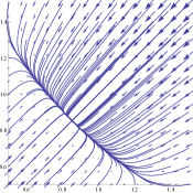
(a) $a=2$

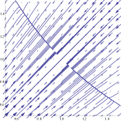
(b) $a=e$

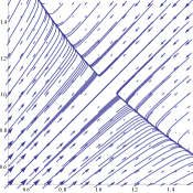
(c) $a=3$

Figure 2: Phase plane pictures

Theorem A.1.

On a scale of Banach spaces $\{\mathbb{B}_{s}:0<s\leq s_{0})$ consider the initial value problem

$$\frac{du(t)}{dt}=Au(t),\quad u(0)=u_{0}\in\mathbb{B}_{s_{0}}$$ (A.1)

where, for each $s\in(0,s_{0})$ fixed and for each pair $s^{\prime},s^{\prime\prime}$ such that $s\leq s^{\prime}<s^{\prime\prime}\leq s_{0}$, $A:\mathbb{B}_{s^{\prime\prime}}\to\mathbb{B}_{s^{\prime}}$ is a linear mapping so that there is an $M>0$ such that for all $u\in\mathbb{B}_{s^{\prime\prime}}$

$$\|Au\|_{s^{\prime}}\leq\frac{M}{s^{\prime\prime}-s^{\prime}}\|u\|_{s^{\prime\prime}}.$$

Here $M$ is independent of $s^{\prime},s^{\prime\prime}$ and $u$, however it might depend continuously on $s,s_{0}$.

Then, for each $s\in(0,s_{0})$, there is a constant $\delta>0$ (i.e., $\delta=\frac{1}{eM}$) such that there is a unique function $u:\bigl{[}0,\delta(s_{0}-s)\bigr{)}\rightarrow\mathbb{B}_{s}$ which is continuously differentiable on $\bigl{(}0,\delta(s_{0}-s)\bigr{)}$ in $\mathbb{B}_{s}$, $Au\in\mathbb{B}_{s}$, and solves (A.1) in the time-interval $0\leq t<\delta(s_{0}-s)$.

Theorem A.2.

On a scale of Banach spaces $\{\mathbb{B}_{s}:0<s\leq s_{0})$ consider a family of initial value problems

$$\frac{du_{\varepsilon}(t)}{dt}=A_{\varepsilon}u_{\varepsilon}(t),\quad u_{\varepsilon}(0)=u_{\varepsilon}\in\mathbb{B}_{s_{0}},\quad\varepsilon\geq 0,$$ (A.2)

where, for each $s\in(0,s_{0})$ fixed and for each pair $s^{\prime},s^{\prime\prime}$ such that $s\leq s^{\prime}<s^{\prime\prime}\leq s_{0}$, $A_{\varepsilon}:\mathbb{B}_{s^{\prime\prime}}\to\mathbb{B}_{s^{\prime}}$ is a linear mapping so that there is an $M>0$ such that for all $u\in\mathbb{B}_{s^{\prime\prime}}$

$$\|A_{\varepsilon}u\|_{s^{\prime}}\leq\frac{M}{s^{\prime\prime}-s^{\prime}}\|u\|_{s^{\prime\prime}}.$$

Here $M$ is independent of $\varepsilon,s^{\prime},s^{\prime\prime}$ and $u$, however it might depend continuously on $s,s_{0}$. Assume that there is a $p\in\mathbb{N}$ and for each $\varepsilon>0$ there is an $N_{\varepsilon}>0$ such that for each pair $s^{\prime},s^{\prime\prime}$, $s\leq s^{\prime}<s^{\prime\prime}\leq s_{0}$, and all $u\in\mathbb{B}_{s^{\prime\prime}}$

$$\|A_{\varepsilon}u-A_{0}u\|_{s^{\prime}}\leq\sum_{k=1}^{p}\frac{N_{\varepsilon}}{(s^{\prime\prime}-s^{\prime})^{k}}\|u\|_{s^{\prime\prime}}.$$

In addition, assume that $\lim_{\varepsilon\rightarrow 0}N_{\varepsilon}=0$ and $\lim_{\varepsilon\rightarrow 0}\|u_{\varepsilon}(0)-u_{0}(0)\|_{s_{0}}=0$.

Then, for each $s\in(0,s_{0})$, there is a constant $\delta>0$ (i.e., $\delta=\frac{1}{eM}$) such that there is a unique solution $u_{\varepsilon}:\left[0,\delta(s_{0}-s)\right)\to\mathbb{B}_{s}$, $\varepsilon\geq 0$, to each initial value problem (A.2) and for all $t\in\left[0,\delta(s_{0}-s)\right)$ we have

$$\lim_{\varepsilon\rightarrow 0}\|u_{\varepsilon}(t)-u_{0}(t)\|_{s}=0.$$

References

- [1] S. Albeverio, Y. Kondratiev, and M. Röckner. Analysis and geometry on configuration spaces. J. Funct. Anal., 154(2):444–500, 1998.
- [2] E. A. Carlen, M. C. Carvalho, R. Esposito, J. L. Lebowitz, and R. Marra. Displacement convexity and minimal fronts at phase boundaries. Arch. Ration. Mech. Anal., 194(3):823–847, 2009.
- [3] E. A. Carlen, M. C. Carvalho, R. Esposito, J. Lebowitz, and R. Marra. Phase transitions in equilibrium systems: Microscopic models and mesoscopic free energies. Molecular Physics, 103:3141–3151, 2005.
- [4] A. De Masi, I. Merola, E. Presutti, and Y. Vignaud. Potts models in the continuum. Uniqueness and exponential decay in the restricted ensembles. J. Stat. Phys., 133(2):281–345, 2008.
- [5] A. De Masi, I. Merola, E. Presutti, and Y. Vignaud. Coexistence of ordered and disordered phases in Potts models in the continuum. J. Stat. Phys., 134(2):243–306, 2009.
- [6] D. Finkelshtein. Measures on two-component configuration spaces. Condensed Matter Physics, 12(1):5–18, 2009.
- [7] D. Finkelshtein, Y. Kondratiev, and O. Kutoviy. Vlasov scaling for stochastic dynamics of continuous systems. J. Stat. Phys., 141(1):158–178, 2010.
- [8] D. Finkelshtein, Y. Kondratiev, and O. Kutoviy. Vlasov scaling for the Glauber dynamics in continuum. Infin. Dimens. Anal. Quantum Probab. Relat. Top., 14(4):537–569, 2011.
- [9] D. Finkelshtein, Y. Kondratiev, and O. Kutoviy. Correlation functions evolution for the Glauber dynamics in continuum. Semigroup Forum, 85:289–306, 2012.
- [10] D. Finkelshtein, Y. Kondratiev, and O. Kutoviy. Semigroup approach to non-equilibrium birth-and-death stochastic dynamics in continuum. J. Funct. Anal., 262(3):1274–1308, 2012.
- [11] D. Finkelshtein, Y. Kondratiev, and M. J. Oliveira. Glauber dynamics in the continuum via generating functionals evolution. Complex Anal. Oper. Theory, 6(4):923–945, 2012.
- [12] D. Finkelshtein, Y. Kondratiev, and M. J. Oliveira. Markov evolutions and hierarchical equations in the continuum. II. Multicomponent systems. Rep. Math. Phys., 71(1):123–148, 2013.
- [13] H.-O. Georgii and O. Häggström. Phase transition in continuum Potts models. Comm. Math. Phys., 181(2):507–528, 1996.
- [14] H.-O. Georgii, S. Miracle-Sole, J. Ruiz, and V. A. Zagrebnov. Mean-field theory of the Potts gas. J. Phys. A, 39(29):9045–9053, 2006.
- [15] M. W. Hirsch, S. Smale, and R. L. Devaney. Differential Equations, Dynamical Systems, and an Introduction to Chaos, volume 60 of Pure and Applied Mathematics (Amsterdam). Elsevier/Academic Press, Amsterdam, second edition, 2004.
- [16] C. Kipnis and C. Landim. Scaling Limits of Interacting Particle Systems, volume 320 of Grundlehren der Mathematischen Wissenschaften. Springer-Verlag, Berlin, 1999.
- [17] Y. Kondratiev and T. Kuna. Harmonic analysis on configuration space. I. General theory. Infin. Dimens. Anal. Quantum Probab. Relat. Top., 5(2):201–233, 2002.
- [18] Y. Kondratiev, T. Kuna, and M. J. Oliveira. Analytic aspects of Poissonian white noise analysis. Methods Funct. Anal. Topology, 8(4):15–48, 2002.
- [19] Y. Kondratiev, T. Kuna, and M. J. Oliveira. Holomorphic Bogoliubov functionals for interacting particle systems in continuum. J. Funct. Anal., 238(2):375–404, 2006.
- [20] S. G. Krantz. Function Theory of Several Complex Variables. Pure and Applied Mathematics. John Wiley & Sons, 1982.
- [21] T. Kuna. Studies in Configuration Space Analysis and Applications. PhD Thesis, Bonner Mathematische Schriften [Bonn Mathematical Publications], Nr. 324. Universität Bonn Mathematisches Institut, Bonn, 1999.
- [22] J. Lebowitz and E. Lieb. Phase transition in a continuum classical system with finite interactions. Physics Letters A, 39, 98–100, 1972
- [23] E. Presutti. Scaling Limits in Statistical Mechanics and Microstructures in Continuum Mechanics. Theoretical and Mathematical Physics. Springer, Berlin, 2009.
- [24] D. Ruelle. Existence of a phase transition in a continuous classical system. Phys. Rev. Letters, 27:1040–1041, 1971.
- [25] H. Spohn. Kinetic equations from Hamiltonian dynamics: Markovian limits. Rev. Modern Phys., 52(3):569–615, 1980.
- [26] B. Widom and J. Rowlinson. New model for the study of liquid-vapor phase transitions. J. Chem. Phys., 52(4):1670–1684, 1970.