py-oopsi: the python implementation of the fast-oopsi algorithm

Abstract

Fast-oopsi was developed by joshua vogelstein in 2009, which is now widely used to extract neuron spike activities from calcium fluorescence signals. Here, we propose detailed implementation of the fast-oopsi algorithm in python programming language. Some corrections are also made to the original fast-oopsi paper.

I Fast-oopsi, a brief view

Oopsi, from vogelstein [1, 2], is a family of optimal optical spike inference algorithms. Here, we focus on the development of the fast-oopsi, which was originally published in [2]. We will port the MATLAB implementation to python. Sec II, III, IV, V and VI are digests from the original paper by vogelstein [1].

The python implementation, py-oopsi, can be obtained at https://github.com/liubenyuan/py-oopsi.

II Calcium fluorescence model

Let $\mathbf{{F}}$ be a one-dimensional fluorescence trace. At time $t$, the fluorescence measurement $F_{t}$ is a linear Gaussian function of the intracellular calcium concentration $[\mathrm{Ca}^{2+}]_{t}$ at that time:

$$F_{t}=\alpha[\mathrm{Ca}^{2+}]_{t}+\beta+e_{t},\qquad e_{t}\sim\mathcal{N}(0,\sigma^{2})$$ (1)

$\alpha$ determines the scale of the signal, $\beta$ absorbs the offset. $\alpha$ and $\beta$ may be learned independently per neuron. The noise $e_{t}$ is assumed to be i.i.d distributed.

The calcium concentration jumps $A$ $\mu$M after each spike and decays back down to baseline $C_{b}$ $\mu$M, with time constant $\tau$,

$$[\mathrm{Ca}^{2+}]_{t+1}=(1-\Delta/\tau)[\mathrm{Ca}^{2+}]_{t}+(\Delta/\tau)C_{b}+An_{t},$$ (2)

where $\Delta$ is the frame interval. The scale $A$ and $\alpha$, baseline $C_{b}$ and $\beta$ are not identifiable, therefore, we may let $A=1$ and $C_{b}=0$ without loss of generality. $n_{t}$ indicates the number of times the neuron spiked in time $t$, we may also write it as a delta function $\delta_{t}$.

Finally, letting $\gamma=(1-\Delta/\tau)$, we have

$$C_{t}=\gamma C_{t-1}+n_{t}$$ (3)

and (the filtering model)

$$C[z]=\frac{1}{1-\gamma z^{-1}}N[z]$$ (4)

Note that $C_{t}$ does not refer to the absolute intracellular concentration, but rather, a relative measure[2]. The simulated calcium trace can be generated if we synthetically generate $n_{t}$ from a probability distribution. To complete the generative model, we assume spikes are sampled according to a Poisson distribution,

$$n_{t}\sim\text{Poisson}(\lambda\Delta)$$ (5)

where $\lambda\Delta$ is the expected firing rate per bin, $\Delta$ is included to ensure that the expected firing rate is independent of the frame rate[2].

III Bayes Model

We aim to find the most likely spike trains $\hat{\mathbf{{n}}}$ given the fluorescence $\mathbf{{F}}$,

$$\hat{\mathbf{{n}}}=\operatorname*{arg\,max}_{n_{t}\in\mathcal{N}_{0},\forall t}p(\mathbf{{n}}|\mathbf{{F}})$$ (6)

Using Bayes’ rule,

$$p(\mathbf{{n}}|\mathbf{{F}})=\frac{1}{p(\mathbf{{F}})}\cdot p(\mathbf{{F}}|\mathbf{{n}})p(\mathbf{{n}})$$ (7)

given that $p(\mathbf{{F}})$ merely scales the results, we rewrite (6) as,

$$\hat{\mathbf{{n}}}=\operatorname*{arg\,max}_{n_{t}\in\mathcal{N}_{0},\forall t}p(\mathbf{{F}}|\mathbf{{n}})p(\mathbf{{n}})$$ (8)

and we already have,

$$p(\mathbf{{F}}|\mathbf{{n}}) =p(\mathbf{{F}}|\mathbf{{C}})=\prod p(F_{t}|C_{t}),$$ (9)

$$p(\mathbf{{n}}) =\prod p(n_{t}),$$ (10)

where,

$$p(F_{t}|C_{t}) =\mathcal{N}(\alpha C_{t}+\beta,\sigma^{2}),$$ (11)

$$p(n_{t}) =\mathrm{Poisson}(\lambda\Delta)$$ (12)

The Poisson distribution penalize sparsity (a sparse prior).

Finally, we have the cost function,

$$\hat{\mathbf{{n}}} =\operatorname*{arg\,max}_{n_{t}\in\mathcal{N}_{0}}\prod_{t=1}^{T}\frac{1}{\sqrt{2\pi\sigma^{2}}}\exp\left\{-\frac{1}{2}\frac{(F_{t}-\alpha C_{t}-\beta)^{2}}{\sigma^{2}}\right\}\frac{\exp\left\{-\lambda\Delta\right\}(\lambda\Delta)^{n_{t}}}{n_{t}!}$$ (13)

$$=\operatorname*{arg\,max}_{n_{t}\in\mathcal{N}_{0}}\sum_{t=1}^{T}-\frac{1}{2\sigma^{2}}(F_{t}-\alpha C_{t}-\beta)^{2}+n_{t}\ln\lambda\Delta-\ln n_{t}!$$ (14)

However, solving for this discretized optimization problem is computational intractable.

IV Approximate Bayes Filter

We can approximate the Poisson distribution with an exponential distribution of the same mean,

$$\frac{\exp\{-\lambda\Delta\}(\lambda\Delta)^{n_{t}}}{n_{t}!}\rightarrow(\lambda\Delta)\exp\{-n_{t}\lambda\Delta\}$$ (15)

and consequently,

$$\hat{\mathbf{{n}}}=\operatorname*{arg\,max}_{n_{t}>0}\sum_{t=1}^{T}-\frac{1}{2\sigma^{2}}(F_{t}-\alpha C_{t}-\beta)^{2}-n_{t}\lambda\Delta$$ (16)

note that $n_{t}\in\mathcal{N}_{0}$ has been replaced by $n_{t}>0$, since exponential distribution can yield any nonnegative number[2]. The exponential approximation imposes a sparsening effect, and also, it makes the optimization problem concave in $\mathbf{{C}}$, meaning that any gradient descent algorithm guarantees achieving the global maxima (because there are no local minima).

We may further drop the constraint (nonnegative) by adopting interior point method,

$$\hat{\mathbf{{n}}}=\operatorname*{arg\,max}_{n_{t}}\sum_{t=1}^{T}-\frac{1}{2\sigma^{2}}(F_{t}-\alpha C_{t}-\beta)^{2}-n_{t}\lambda\Delta+z\ln n_{t}$$ (17)

where we add a weighted barrier term that approaches $-\infty$ as $n_{t}$ approaches zero, by solving for a series of $z$ going down to nearly zero. The goal is to efficiently solve,

$$\hat{\mathbf{{C}}}=\operatorname*{arg\,max}_{C}\sum_{t=1}^{T}-\frac{1}{2\sigma^{2}}(F_{t}-\alpha C_{t}-\beta)^{2}-(C_{t}-\gamma C_{t-1})\lambda\Delta+z\ln(C_{t}-\gamma C_{t-1})$$ (18)

this cost function is twice differentiable, one can use the Newton-Raphson technique to ascend the surface.

V Matrix Notation and the Newton-Raphson solver

To proceed, we have

$$\mathbf{{M}}\mathbf{{C}}=\begin{bmatrix}-\lambda&1&0&0&\cdots&0\\ 0&-\lambda&1&0&\cdots&0\\ \vdots&\ddots&\ddots&\ddots&\ddots&\vdots\\ 0&\cdots&0&-\lambda&1&0\\ 0&\cdots&0&0&-\lambda&1\end{bmatrix}\begin{bmatrix}C_{1}\\ C_{2}\\ \vdots\\ C_{T-1}\\ C_{T}\end{bmatrix}=\begin{bmatrix}n_{1}\\ n_{2}\\ \vdots\\ n_{T-1}\end{bmatrix}$$ (19)

$\mathbf{{M}}$ is a $(T-1)\times T$ matrix. Now letting $\mathbf{{1}}$ be a $(T-1)\times 1$ column vector, $\bm{\lambda}=(\lambda\Delta)\mathbf{{1}}$, $\bm{\alpha}$ and $\bm{\beta}$ a $T$-dimensional vector, $\odot$ to indicate element-wise operations, then

$$\hat{\mathbf{{C}}}=\operatorname*{arg\,max}_{\mathbf{{MC}}\geq_{\odot}\mathbf{{0}}}-\frac{1}{2\sigma^{2}}\|\mathbf{{F}}-\bm{\alpha}\mathbf{{C}}-\bm{\beta}\|_{2}^{2}-(\mathbf{{MC}})^{T}\bm{\lambda}+z\ln_{\odot}(\mathbf{{MC}})^{T}\mathbf{{1}}$$ (20)

We instead iteratively minimize the cost function $\mathcal{L}$ (called post in our python implementation) where,

$$\hat{\mathbf{{C}}}_{z}=\operatorname*{arg\,min}_{\mathbf{{C}}}\mathcal{L},\quad\mathcal{L}=\frac{1}{2\sigma^{2}}\|\mathbf{{F}}-\bm{\alpha}\mathbf{{C}}-\bm{\beta}\|_{2}^{2}+(\mathbf{{MC}})^{T}\bm{\lambda}-z\ln_{\odot}(\mathbf{{MC}})^{T}\mathbf{{1}}$$ (21)

$\mathcal{L}$ is convex, when using Newton-Raphson method to descend a surface, one iteratively computes the gradient $\mathbf{{g}}=\nabla\mathcal{L}$ (first derivative) and Hessian $\mathbf{{H}}=\nabla^{2}\mathcal{L}$ (second derivative) of the argument to be optimized. Then, $\mathbf{{C}}=\mathbf{{C}}-s\mathbf{{d}}$, where $s$ is the step size and $\mathbf{{d}}$ is the step direction by solving $\mathbf{{H}}\mathbf{{d}}=\mathbf{{g}}$. The gradient and Hessian, with respect to $\mathbf{{C}}$, are

$$\mathbf{{g}} =-\frac{\bm{\alpha}}{\sigma^{2}}(\mathbf{{F}}-\bm{\alpha}\mathbf{{C}}-\bm{\beta})+\mathbf{{M}}^{T}\bm{\lambda}-z\mathbf{{M}}^{T}(\mathbf{{MC}})_{\odot}^{-1}$$ (22)

$$\mathbf{{H}} =\frac{\alpha^{2}}{\sigma^{2}}\mathbf{{I}}+z\mathbf{{M}}^{T}(\mathbf{{MC}})_{\odot}^{-2}\mathbf{{M}}$$ (23)

$s$ is found via backtracking linesearches. $\mathbf{{M}}$ is bidiagonal, so $\mathbf{{H}}$ is tridiagonal, $\mathbf{{d}}=\mathbf{{H}}^{-1}\mathbf{{g}}$ can be efficiently implemented in matlab by assuming $\mathbf{{H}}$ is a sparse matrix. In python, we may use sparse linsolvers (linsolve.spsolve) to efficiently find $\mathbf{{d}}$. Once $\hat{\mathbf{{C}}}$ is obtained, it is a simple linear transform to obtain $\hat{\mathbf{{n}}}$, via $\hat{\mathbf{{n}}}=\mathbf{{M}}\hat{\mathbf{{C}}}$. We will normalize $\mathbf{{n}}$ by $\mathbf{{n}}=\mathbf{{n}}/\mathrm{max}(\mathbf{{n}})$ after convergence.

VI Parameters initialize and update

The parameters $\bm{\theta}=\{\alpha,\beta,\sigma,\gamma,\lambda\}$ are unknown. We may use pseudo expectation-maximization method, (1), initialize the parameters, (2) recursively computes $\hat{\mathbf{{n}}}$ and updating $\bm{\theta}$ given the new $\hat{\mathbf{{n}}}$ until the convergence is met.

The scale of $\mathbf{{F}}$ relative to $\mathbf{{n}}$ is arbitrary, therefore, $\mathbf{{F}}$ is firstly detrended, and then linearly mapped between $0$ and $1$.

$$\mathbf{{F}}=\mathrm{detrend}(\mathbf{{F}}),\quad\mathbf{{F}}=(\mathbf{{F}}-F_{min})/(F_{max}-F_{min}),$$ (24)

Next, because spiking is sparse in many experimental settings, $\mathbf{{F}}$ tends to be around baseline, $\beta$ is set to the median of $\mathbf{{F}}$. We use median absolute deviation (MAD) and correction factor $K$, as a robust normal scale estimator of $\mathbf{{F}}$ where $K=1.4826$. Previous works showed that the results $\hat{\mathbf{{n}}}$ and $\hat{\mathbf{{C}}}_{z}$ are robust to minor variations in the time constant, we let $\gamma=1-\Delta$. Finally, $\lambda$ is set to $1$Hz, which is between baseline and evoked spike rate for data of interest .

$$\alpha =1,$$ (25)

$$\beta =\mathrm{median}(\mathbf{{F}}),$$ (26)

$$\sigma =\mathrm{MAD}(\mathbf{{F}})\cdot K=\mathrm{median}(|\mathbf{{F}}-\beta|)\cdot K,\quad K=1.4826$$ (27)

$$\gamma =1-\Delta/(1\mathrm{sec}),$$ (28)

$$\lambda =1\mathrm{Hz}$$ (29)

Then, given $\hat{\mathbf{{C}}}$ and $\hat{\mathbf{{n}}}$, we may (approximately) update $\bm{\theta}$ by,

$$\hat{\bm{\theta}}\approx\operatorname*{arg\,max}_{\bm{\theta}}p(\mathbf{{F}},\hat{\mathbf{{C}}}|\bm{\theta})=\operatorname*{arg\,max}_{\bm{\theta}}\ln p(\mathbf{{F}}|\hat{\mathbf{{C}}};\{\alpha,\beta,\sigma\})+\ln p(\hat{\mathbf{{n}}}|\lambda)$$ (30)

where,

$$\hat{\lambda} =\operatorname*{arg\,max}_{\lambda>0}\sum_{i=1}^{T}\left[\ln(\lambda\Delta)+\hat{n_{t}}\lambda\Delta\right]$$ (31)

$$\{\hat{\alpha},\hat{\beta},\hat{\sigma}\} =\operatorname*{arg\,max}_{\alpha,\beta,\sigma>0}\sum_{i=1}^{T}\left[-\frac{1}{2}\ln(2\pi\sigma^{2})-\frac{1}{2}\left(\frac{F_{t}-\alpha C_{t}-\beta}{\sigma}\right)^{2}\right]$$ (32)

We have (by taking the derivatives and letting them equal zero),

$$\hat{\lambda} =\frac{T}{\Delta\sum_{t}n_{t}},$$ (33)

$$\hat{\alpha} =1,$$ (34)

$$\hat{\beta} =\frac{\sum_{t}(F_{t}-C_{t})}{T},$$ (35)

$$\hat{\sigma}^{2} =\frac{\sum_{t}(F_{t}-C_{t}-\beta)^{2}}{T}=\frac{\|\mathbf{{F}}-\mathbf{{C}}-\bm{\beta}\|_{2}^{2}}{T}$$ (36)

where $\hat{\lambda}$ is the inverse of the inferred firing rate, $\hat{\alpha}$ can be set to $1.0$ because the scale of $\mathbf{{C}}$ is arbitrary, $\hat{\beta}$ is the mean bias, $\hat{\sigma}$ is the root-mean-square of the residual error.

VII Implementation of oopsi

Matlab implementation is available, here we focus on the python migrant, and correct some typos in [2] as needed. The python code itself explains all, see IV, V, and VI for detailed documentary. Pseudo code can be found in Algo 1. Algo 2 describe the subroutine MAP, Algo 3 describe the subroutine update.

Algorithm 1 Pseudo code (python) for fast-oopsi

1:  Initialize parameters $\mathbf{{P}}$: $\mathbf{{F}}=\mathrm{detrend}(\mathbf{{F}})$, $\mathbf{{F}}=(\mathbf{{F}}-\mathrm{min}(\mathbf{{F}}))/(\mathrm{max}(\mathbf{{F}})-\mathrm{min}(\mathbf{{F}}))$, $\alpha=1.0$, $\beta=\mathrm{median}(\mathbf{{F}})$, $\lambda=1.0$, $\gamma=1-\Delta$, $\sigma=\mathrm{MAD}(\mathbf{{F}})\cdot 1.4826$, $T=\mathrm{len}(\mathbf{{F}})$

2:  one-shot Newton-Raphson $\mathbf{{n}}$, $\mathbf{{C}}$, $\mathcal{L}$ = MAP($\mathbf{{F}}$,$\mathbf{{P}}$), see Algo 2.

3:  for $i$ in $1\cdots\mathrm{iterMax}$ do

4:     update parameters $\mathbf{{P}}$ = update($\mathbf{{n}}$,$\mathbf{{C}}$,$\mathbf{{F}}$,$\mathbf{{P}}$), see Algo 3.

5:     iterative through $\mathbf{{n}}$, $\mathbf{{C}}$, $\mathcal{L}$ = MAP($\mathbf{{F}}$,$\mathbf{{P}}$),

6:     let $\mathcal{L}^{(k)}=\{\mathcal{L}_{1},\cdots,\mathcal{L}_{k}\}$

7:     if $|\frac{\mathcal{L}_{i}-\mathcal{L}_{i-1}}{\mathcal{L}_{i}}|<\mathrm{ltol}$ or $\mathrm{any}(|\mathcal{L}^{(i)}-\mathcal{L}_{i}|)<\mathrm{gtol}$ then

8:        break

9:     end if

10:  end for

Algorithm 2 Pseudo code of subroutine MAP

1:  Initialize $\mathbf{{n}}=0.01\mathbf{{1}}$

2:  Initialize $\mathbf{{C}}(z)=1/(1-\gamma)\mathbf{{N}}(z)$

3:  Initialize $\bm{\lambda}=\lambda\Delta\mathbf{{1}}$

4:  for $z=1.0$, $z>1e-13$, $z=z/10$ do

5:     calculate $\mathcal{L}_{z}$

6:     while $s>1e-3$ or $\|\mathbf{{d}}\|>5e-2$ do

7:        Calculate $\mathbf{{g}}$, $\mathbf{{H}}$ and $\mathbf{{d}}=\mathrm{spsolve}(\mathbf{{H}},\mathbf{{g}})$

8:        Find $s$ : $\mathbf{{h}}=-\mathbf{{n}}/(\mathbf{{M}}\mathbf{{d}})$, $s=\min(0.99\mathbf{{s}}[\mathbf{{s}}>0],1.0)$

9:        Initialize $\mathcal{L}_{s}=\mathcal{L}_{z}+1$

10:        while $\mathcal{L}_{s}>\mathcal{L}_{z}+1e-7$ do

11:           $\mathbf{{C}}=\mathbf{{C}}+s\mathbf{{d}}$

12:           $\mathbf{{n}}=\mathbf{{MC}}$

13:           update $\mathcal{L}_{s}$

14:           decrease $s=s/5.0$

15:           if $s<1e-20$ then

16:              break

17:           end if

18:        end while

19:     end while

20:  end for

Algorithm 3 Pseudo code of subroutine update

1:  $\alpha=1.0$

2:  $\beta=\sum_{i}(F_{i}-C_{i})/T$

3:  $\sigma^{2}=\|\mathbf{{F}}-\alpha\mathbf{{C}}-\beta\|_{2}^{2}/T$

4:  $\lambda=T/(\Delta\sum_{i}n_{i})$

VIII Wiener filter (linear regression, simple convex optimization)

In the wiener filter, we approximate the Poisson distribution with a Gaussian distribution,

$$p(n_{t})\sim\mathcal{N}(\lambda\Delta,\lambda\Delta)$$ (37)

then, the MAP estimator yields,

$$\hat{\mathbf{{n}}}=\operatorname*{arg\,max}_{n_{t}}\sum_{t=1}^{T}\left[-\frac{1}{2\sigma^{2}}(F_{t}-\alpha C_{t}-\beta)^{2}-\frac{1}{2\lambda\Delta}(n_{t}-\lambda\Delta)^{2}\right]$$ (38)

and its matrix notation,

$$\hat{\mathbf{{C}}}=\operatorname*{arg\,max}_{\mathbf{{C}}}-\frac{1}{2\sigma^{2}}\|\mathbf{{F}}-\alpha\mathbf{{C}}-\beta\mathbf{{1}}\|_{2}^{2}-\frac{1}{2\lambda\Delta}\|\mathbf{{MC}}-\lambda\Delta\mathbf{{1}}\|_{2}^{2}$$ (39)

which is quadratic, concave in $\mathbf{{C}}$.

Finally, we aim to optimize (minimize, quadratic, convex optimization),

$$\hat{\mathbf{{C}}}=\operatorname*{arg\,min}_{\mathbf{{C}}}\mathcal{L},\quad\mathcal{L}=\frac{1}{2\sigma^{2}}\|\mathbf{{F}}-\alpha\mathbf{{C}}-\beta\mathbf{{1}}\|_{2}^{2}+\frac{1}{2\lambda\Delta}\|\mathbf{{MC}}-\lambda\Delta\mathbf{{1}}\|_{2}^{2}$$ (40)

where $\mathcal{L}$ is convex in $\mathbf{{C}}$. Using Newton-Raphson update, we find $\mathbf{{C}}=\mathbf{{C}}-\mathbf{{d}}$, $\mathbf{{H}}\mathbf{{d}}=\mathbf{{g}}$ and $\mathbf{{g}}=\nabla\mathcal{L}$, $\mathbf{{H}}=\nabla^{2}\mathcal{L}$. The gradient $\mathbf{{g}}$ and Hessian $\mathbf{{H}}$ are,

$$\mathbf{{g}} =-\frac{\alpha}{\sigma^{2}}(\mathbf{{F}}-\alpha\mathbf{{C}}-\beta\mathbf{{1}})+\frac{1}{\lambda\Delta}\left[\mathbf{{M}}^{T}(\mathbf{{MC}})+\lambda\Delta\mathbf{{M}}^{T}\mathbf{{1}}\right]$$ (41)

$$\mathbf{{H}} =\frac{\alpha^{2}}{\sigma^{2}}\mathbf{{I}}+\frac{1}{\lambda\Delta}\mathbf{{M}}^{T}\mathbf{{M}}$$ (42)

In the python implementation, we let $\alpha=1.0$ and $\beta=0.0$. Pseudo code can be found in Algo 4.

Algorithm 4 Pseudo code (python) for wiener filter

1:  Initialize $\mathbf{{F}}=(\mathbf{{F}}-\mathrm{mean}(\mathbf{{F}}))/\mathrm{max}(|\mathbf{{F}}|)$, $\sigma=0.1\|\mathbf{{F}}\|_{2}$

2:  Calculate $\mathcal{L}_{0}$

3:  for $i$ in $1\cdots$ iterMax do

4:     Calculate $\mathbf{{g}}$, $\mathbf{{H}}$ and $\mathbf{{d}}=\mathrm{spsolve}(\mathbf{{H}},\mathbf{{g}})$

5:     Calculate $\mathbf{{C}}=\mathbf{{C}}-\mathbf{{d}}$

6:     Calculate $\mathcal{L}_{i}$

7:     if $\mathcal{L}_{i}<\mathcal{L}_{i-1}+\mathrm{gtol}$ then

8:        $\mathbf{{n}}=\mathbf{{N}}$

9:        $\sigma=\sqrt{\|\mathbf{{F}}-\mathbf{{C}}\|_{2}^{2}/T}$

10:     end if

11:  end for

12:  $\mathbf{{n}}=\mathbf{{n}}/\mathrm{max}(\mathbf{{n}})$

IX Simulation Results

We generated synthetic calcium traces with $T=2000$, $\Delta=20$ms, $\lambda=0.1$, $\tau=1.5$. Randomized noise were added with $0.2$ standard deviation. Py-oopsi and wiener filter are used to reconstruct the spikes from calcium fluorescence, where only $\Delta$ is known a prior. The results are shown in Figure 1

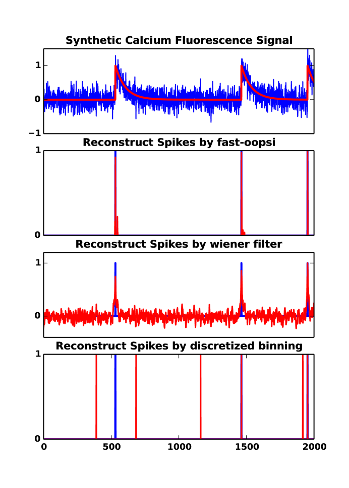
Figure 1: Reconstruct spikes from calcium fluorescence. (a) The synthetic calcium trace. (b), (c), (d) are reconstructed spikes by py-oopsi, wiener filter and discretized binning, respectively.

References

• [1] J. T. Vogelstein, OOPSI: A family of optimal optical spike inference algorithms for inferring neural connectivity from population calcium imaging.   THE JOHNS HOPKINS UNIVERSITY, 2010.
• [2] J. Vogelstein, A. Packer, T. Machado, T. Sippy, B. Babadi, R. Yuste, and L. Paninski, “Fast nonnegative deconvolution for spike train inference from population calcium imaging.” Journal of neurophysiology, vol. 104, no. 6, pp. 3691–3704, 2010.