Development of the method of computer analogy for studying and solving complex nonlinear systems
11institutetext: Dorodnicyn Computing Centre of Russian Academy of Sciences,
11email: aristovvl@yandex.ru,
11email: savthe@gmail.com
Abstract
A method of representation of a solution as segments of the series in powers of the step of the independent variable is expanded for solving complex systems of ordinary differential equations (ODE): the Lorenz system and other systems. A new procedure of reduction of the representation of the solution to a sum of two parts (regular and random) is performed. A shifting procedure is applied in each level of the independent variable to the random part and it acts as the filter that extracts the values to the regular part. In certain cases it is possible to omit the random part and construct the approximation which does not converge but still provides the qualitative information about the full solution (a linear approximation provides a simple exact solution). Evaluation of the error for this case is performed. Constructing the analytical representation of the solutions for these systems by the developed method is presented.
Keywords:
theoretical computer model; digit shifting; the method of computer analogy; nonlinear differential equations1 Introduction
In papers [1-2] we proposed a new approach for solving nonlinear differential equations which utilizes two main principles of storing the numbers in the digital computers: 1) the numbers are represented as the segments of a power series; 2) there is a digit shifting procedure. In each level the numerical solution is presented as the segment of a series in the powers of the step of the independent variable. The digit shifting procedure is applied in each level to change the values of the coefficients of the terms so each coefficient would not exceed . We have shown that the digit shifting can produce quasi-random numbers which have been used to exclude the intermediate levels of computations. This method can provide a solution in the explicit form (as a computer provides a solution in the numerical form, after executing many intermediate and ”hidden” operations). Some examples of solving different nonlinear equations and simple systems have been demonstrated.
In the present paper we consider nonlinear systems which have the physical sense. Namely the Van der Pol equation (equivalent to a system of two ODE) and the well-known Lorenz system of the three ODE. We prove that for ODE where the right hand part is a polynomial of degree , it is sufficient to retain the terms up to plus the order of accuracy of the numerical method.
2 The method of computer analogy
2.1 Problem statement
In most cases the nonlinear differential equations can not be solved analytically, but usually they can be solved numerically instead. However one of the main distinctions between analytical and numerical solutions is that the numerical solution is not conceivable without a computer — a physical device which performs routine computations.
Consider the following Cauchy problem:
| (1) |
Let there be a -th order explicit finite-difference scheme which approximates the solution, it can be written as:
where is a step of the independent variable , is determined by function a and by the chosen finite difference method. Note that for the first order method is equivalent to .
When solving the numerical solution the computer acts as a black box, which runs an algorithm and after performing a large amount of steps of the algorithm provides a result as the array of numbers. The computer operations are fairly simple, but due to nonlinearity (in general) of the problem under consideration it is difficult to understand how the values will be changed after few operations.
From a certain point of view the computer solves the numerical analog of the analytical problem, and instead of the analysis and analytical computations it executes an algorithm. But on the other hand we can consider a numerical solution as the independent problem and search for an analytical solution (or approximation) for this particular problem. First, we will formalize the numbers representation in computers. The following aspects are essential: 1) the numbers are stored as the segments of the power series, 2) there is the digit shifting procedure which shifts a part of the value to the left digit.
2.2 Solution representation
The power series in powers of can be obtained from the explicit finite differece scheme and the Taylor expansion.
Theorem 2.1
Let is infinitely differentiable function with bounded derivatives. Then can be represented by the series in powers of :
| (2) |
This follows from the Taylor expansion of at :
Using this expansion we find . Comparison of the coefficients in the sequential layers gives the following recurrent relations:
| (3) |
and so on.
The expansion of can not be truncated after a fixed number of terms because the truncated value will be of a greater order than the accuracy of the finite-difference method, and such a solution would diverge.
Let us construct a procedure of redistribution of the values of the coefficients so that
1) the value of remains unchanged;
2) for any : .
Consider the following example. Let and in -th layer is written as follows:
Let after applying the finite-difference formula we got
The coefficient at is greater than which leads to the eventual divergence. In order to avoid this we apply the digit shifting procedure. It can be done in different ways, but following to how we do it in common positional numeral systems, we take from and add to (at ):
As we see, the value is not changed, but the structure of the value is changed.
The digit shifting procedure allows us to hold the values when applying the numerical scheme which would otherwise be truncated.
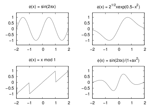
Now we will show how the shifting procedure can be constructed. To guarantee that series (2) is convergent we will restrain the absolute values of by . Let there is a piecewise function that maps to the segment . Consider a function We will refer to it as the shifting function. In Fig. 1 few possible choices of are shown.
Consider the expansion where the absolute values of the coefficients can be greater than :
Let is the shifting function. It should be applied for each coefficient. Let us consider its application for -th coefficient. First of all we must add to it the value shifted from -th coefficient, denote it as . Let us add and subtract the value
Since , we imply the following:
The shifting procedure guarantees that the absolute values of the coefficients of the power series are limited by the value which implies that the series may be truncated.
2.3 General solution representation
Consider series (2). Now, using the digit shifting procedure, we will construct the representation of the solution. Let us denote as and from and on as . Since all coefficients are limited by , we conclude that
thus is of order of . Let us show that can be approximated by with error . Consider the difference . Since , let us expand at
Since the derivatives of are bounded, we obtain that . This yields .
Let us expand at :
| (4) |
Consider the first order explicit finite-difference scheme for (1):
Combining (2) and (4) we obtain:
Then we get:
| (5) |
Theorem 2.2
If the right hand part of ODE is a polynomial of degree , then for the first order explicit scheme .
2.4 Solution splitting
Consider a problem (1). Let there is a solution
| (6) |
As we have already shown the convergence is achieved by applying the shifting functions to constrain the coefficients. But instead of applying the shifting function to each coefficient, we can split the segment of the series into two segments:
| (7) |
| (8) |
This allows to write the solution as the following sum:
where is the order of approximation and is the number of retained terms. These two parts are linked together via a single value shifting.
This approach simplifies constructing the solution. For example, could be equal to and could be the number greater, say , in this case the first term, namely describes the regular part of the solution and the second term would be the quasirandom part.
2.5 The basic shifting function
Let the shifting function is . Consider :
This expression conforms to the congruent random number generator formula:
We assume that coefficients are the uniformly distributed random integer numbers. Therefore the solution can be written as a sum of two parts:
deterministic: ,
random: .
These two parts are linked together by the value . If the probabilities of the values of are known, then we can exclude the intermediate layers of independent variable on which the deterministic part remains unchanged.
3 Linear approximation
Let us see how the method of computer analogy can be used to construct linear analytical approximations which in certain cases can be used to get qualitative (or maybe in some cases the quantitative) information about the solution. Let , thus the solution will contain only two terms. Denote them as and , thus:
Using (3) we get the value in the next layer (let ):
Now we apply the digit shifting procedure:
Let . We will use this shifting function by default. The choice of this function is based on the fact that for it follows that . Then can be written as follows:
Since , then possible values for are .
Comparing the coefficients on sequential layers we get the following reccurent relations:
We see that can be changed only when a non-zero digit shifting occures. Suppose that for several sequential layers equals to zero, so there are no values shifted to coefficient . This implyes that for these layers is constant and grows linearly. When the digit shifting takes place the coefficient changes, that leads to changing of angular coefficient of which is .
When reaches , will become or , this will change and consequently the angular coefficient .
Let us now obtain the formulae for constructing the linear approximation. Let
corresponds to some moment . Suppose equal to zero, so there are no shiftings in the first layers, and there is a shift in layer. Then we imply that for any that .
This means that due to the chosen shifting function for any such that because the absolute value of the argument is less than . This yields the reccurent relation for can be written as follows:
This relation can be written explicitly:
By substituting to we get:
Notice that is the value of time , thus:
This relation holds true for any value of such that , thus
Now we will show the value can be obtained. Denote and consider two cases: and . The first case implies that is linearly grows, the second one implies that is linearly descends. Let then the digit shifting occure when :
Thus
For we will use the smallest integer value of the right hand part, so . By analogy we get the following value for in a case : . And now we need to show how to get the new values of and after the shifting of the digit. Denote them as and . If digit shifting is triggered, is changed according to the shifting function, so:
And is changed on or according to :
4 Examples
Example 1
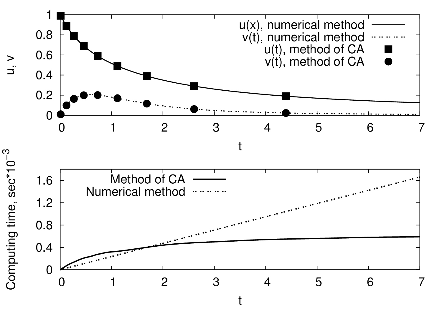
Consider the following Cauchy problem (see [2] for details):
We will use the explicit first-order scheme and represent and as the segments of the series in powers of .
The proposed method allows us to obtain the explicit expressions:
The solutions comparison is shown on Fig. 2.
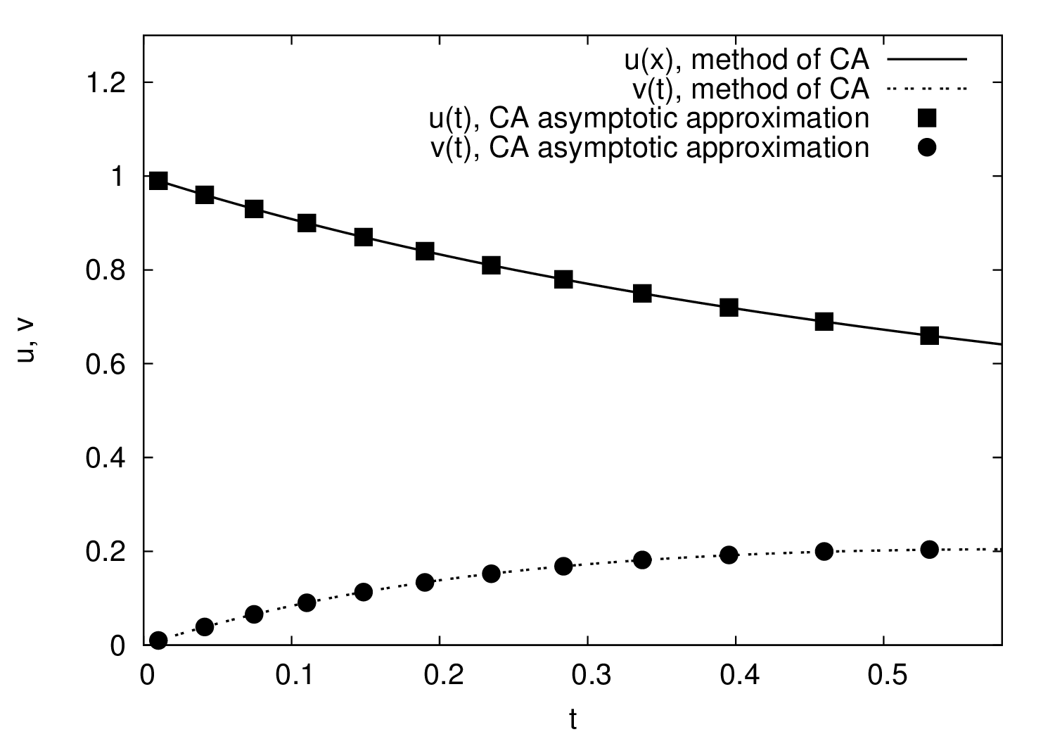
For small values of we can neglect the value (see Fig. 3):
Example 2
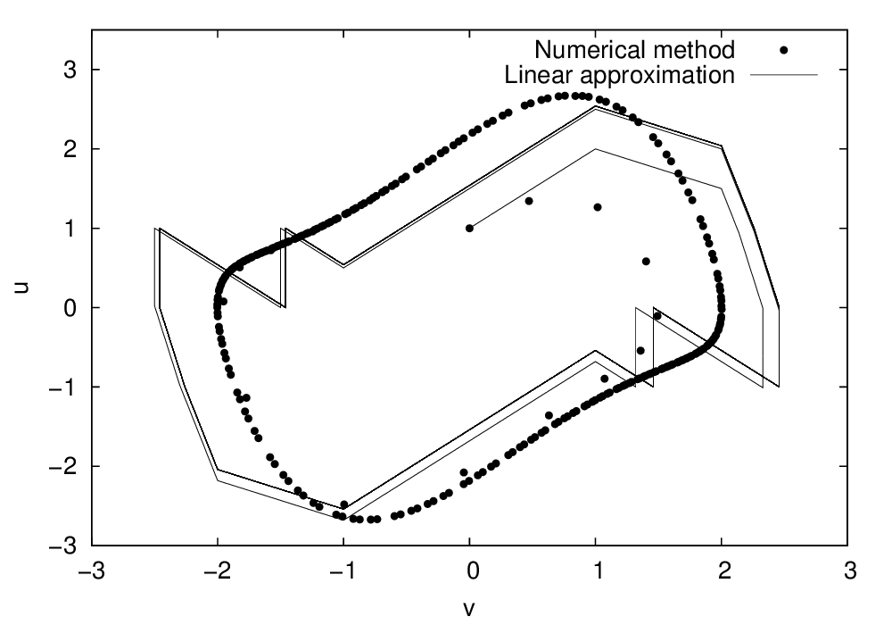
Consider the Van der Pol oscillator which is a second order differential equation:
For this problem there is no analytical solution. Let and rewrite the equation as a system of two differential equations:
Let and . The first order finite difference solution will be as follows:
We will represent the solution as a segment of the series in powers of . Theorem 1 implies that for and it is sufficient to retain terms until and respectively. We will retain only the terms up to for the both functions:
Taking into account the mentioned notices, this solution will not converge, but it is still useful because it allows us to construct linear a approximation which reproduces the behaviour of the solution. Using the finite-difference scheme and the digit shifting procedure we obtain:
Here the shifted values are given by the following expressions:
Let us see how a linear approximation can be constructed. From the initial condition we imply that
Layer 0
From the initial values we obtain and :
Now we calculate and :
A value will be the minimum of values and , namely:
A value defines :
Now we can write the linear approximation in a segment :
To get a solution in the next layer we must compute the initial values for it. Since and the new initial values for and will be and :
The initial values for and are found from and :
Layer 1
By analogy with Layer 0 we compute and :
Find and :
This yields and and we construct the following approximation in a segment :
The initial conditions for the next layer are as follows:
A coefficient is not changed because , so no shifting in occures. We note that this linear solution does not depend on a magnitude of the step .
Layer 2
Values of function are:
And we obtain :
We get the following approximation in a segment :
The explicit solutions can be written in the following table:
Table 1. Piecwise linear approximation for Van der Pol equation.
Figures 4 and 5 demonstrate that this solution converges to the cycle which roughly corresponds to the exact solution.
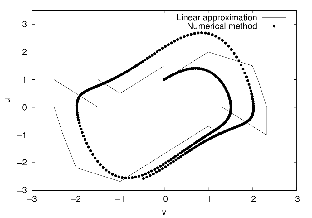
Thus we obtain an analytical solution of the first approximation which provides a qualitative information and reflects some quantitative features.
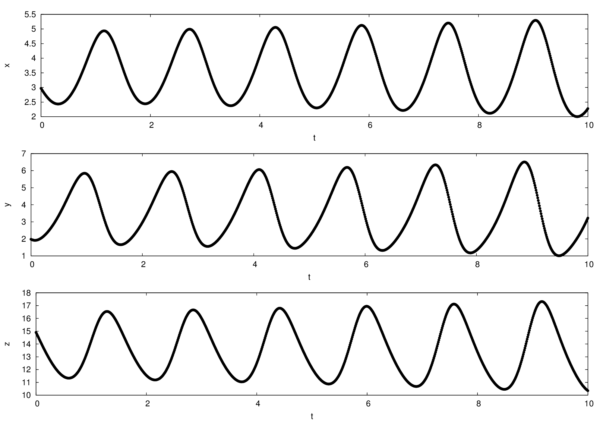
Example 3
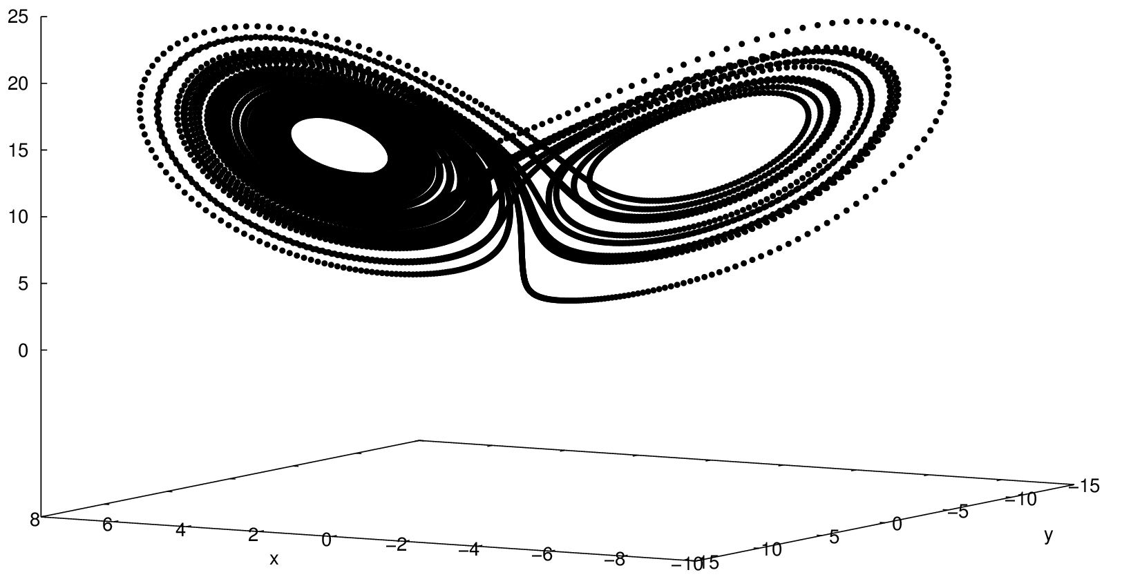
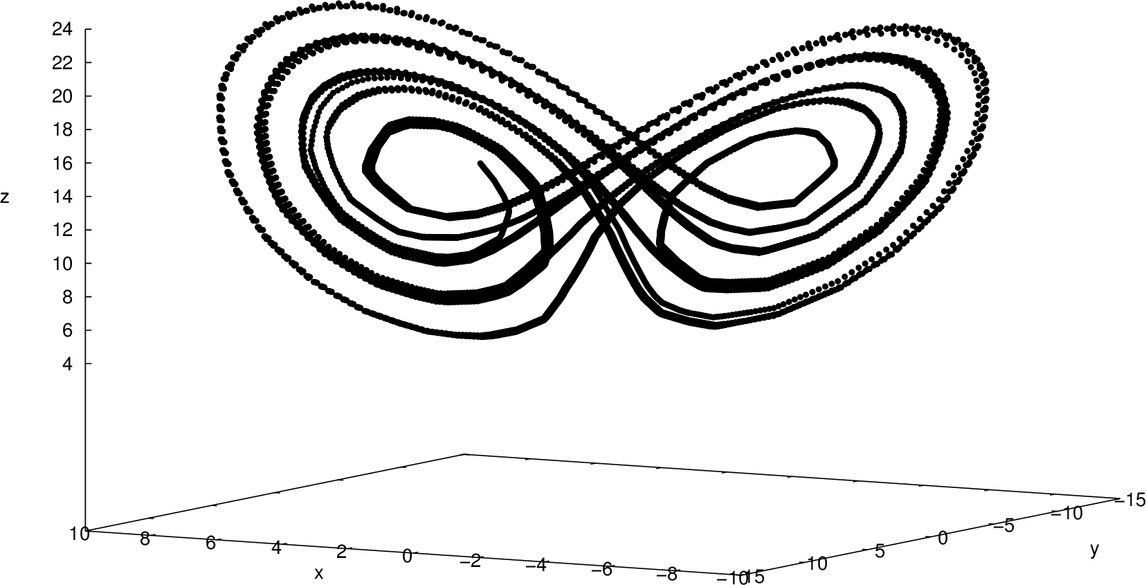
The Lorenz system is given by the following system of nonlinear differential equations:
Let us use the following parameters (which lead to solution with a strange attractor): . We represent according to 2.4:
The finite-difference method and the shifting procedure give:
Simulations confirm that this solution converges to the numerical solution.
Function is shown in Fig. 6. Simulations using method of CA shows the Lorenz attractor behaviour (Fig. 7).
Let us construct the linear approximation. We will retain only the linear terms:
Using the formulae from section 3 we get the following approximation
| t | x | y | z | t | x | y | z |
|---|---|---|---|---|---|---|---|
This solution doesn’t converge, but it still preserves some information about the exact solution. We can see that there is still periodic behavior (Fig. 8) which corresponds to the converging solution.
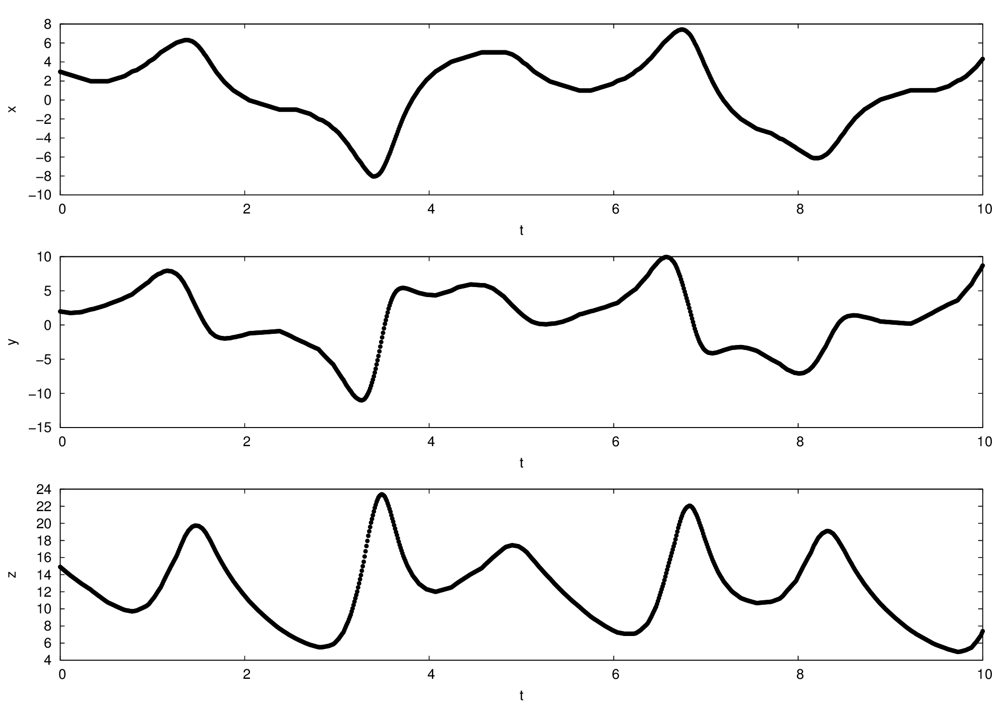
Linear approximation of the Lorenz attractor is shown in Fig. 9.
5 Conclusions
A theoretical model of the computer working with numbers was presented. We analyzed the possibility of formalizing the computer operations, and proposed a representation of a solution in the form of a segment of the series in the powers of the step of the independent variable. This technique involves analytical work for obtaining the probabilities. However, the main steps can be listed as follows: to choose a convergent finite-difference scheme, to find the number of terms to be retained, and to obtain the expressions for the main coefficients in the representation of the solution. The proposed method of the computer analogy allows us to represent the solution of the problem as a convergent series that can be analyzed.
References
- [1] Aristov, V.V., Stroganov, A.V.: Construction of solutions to differential equations by the method of computer analogy. Doklady Mathematics. 82, 151-157 (2010)
- [2] Aristov, V.V., Stroganov, A.V.: A method of formalizing computer operations for solving nonlinear differential equations. Applied Mathematics and Computation. 2012, Vol. 218, p. 8083-8089. doi:10.1016/j.amc.2011.09.029
- [3] Kahaner, D., Mouler, C., Nash, S.: Numerical Methods and Software. Prentice-Hall International Inc, NY, 1989.