Shiba states and zero-bias anomalies in the hybrid normal-superconductor Anderson model

Abstract

Hybrid semiconductor-superconductor systems are interesting melting pots where various fundamental effects in condensed matter physics coexist. For example, when a quantum dot is coupled to a superconducting electrode two very distinct phenomena, superconductivity and the Kondo effect, compete. As a result of this competition, the system undergoes a quantum phase transition when the superconducting gap $\Delta$ is of the order of the Kondo temperature $T_{K}$. The underlying physics behind such transition ultimately relies on the physics of the Anderson model where the standard metallic host is replaced by a superconducting one, namely the physics of a (quantum) magnetic impurity in a superconductor. A characteristic feature of this hybrid system is the emergence of sub-gap bound states, the so-called Yu-Shiba-Rusinov (YSR) states, which cross zero energy across the quantum phase transition, signaling a switching of the fermion parity and spin (doublet or singlet) of the ground state. Interestingly, similar hybrid devices based on semiconducting nanowires with spin-orbit coupling may host exotic zero-energy bound states with Majorana character. Both, parity crossings and Majorana bound states (MBS)s, are experimentally marked by zero bias anomalies in transport, which are detected by coupling the hybrid device with an extra normal contact. We here demonstrate theoretically that this extra contact, usually considered as a non-perturbing tunneling weak probe, leads to nontrivial effects. This conclusion is supported by numerical renormalization group calculations of the phase diagram of an Anderson impurity coupled to both superconducting and normal-state leads. We obtain this phase diagram for an arbitrary ratio $\Delta\over T_{K}$ for the first time, which allows us to analyze relevant experimental scenarios, such as parity crossings as well as novel Kondo features induced by the normal lead, as this ratio changes. Spectral functions at finite temperatures and magnetic fields, which can be directly linked to experimental tunneling transport characteristics, show zero-energy anomalies irrespective of whether the system is in the doublet or singlet regime. We also derive the analytical condition for the occurrence of Zeeman-induced fermion-parity switches in the presence of interactions which bears unexpected similarities with the condition for emergent MBSs in nanowires.

I Motivation and Introduction

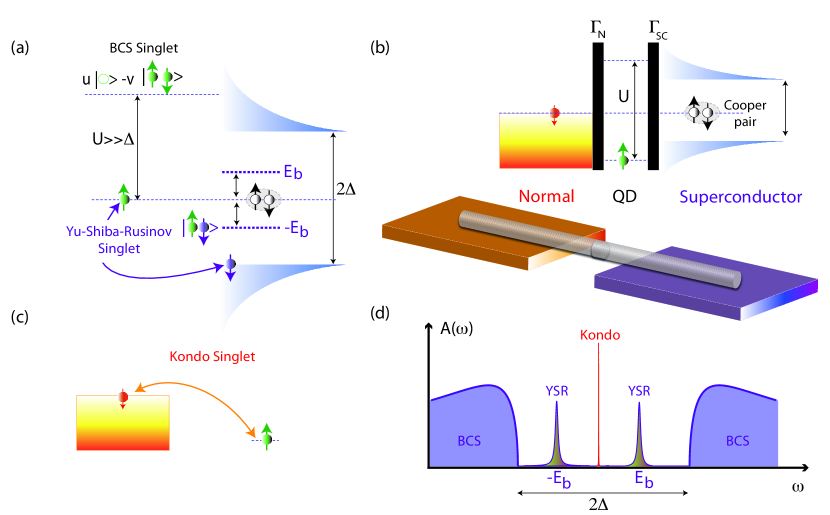
Figure 1: (Color online) (a) Lowest energy many-particle eigenstates of an Anderson impurity coupled to a superconductor with the typical BCS density of states $\sim[(\omega/\Delta)^{2}-1]^{-1/2}$ for large on-site interaction $U\gg\Delta$. The magnetic impurity ground state develops singlet correlations with the quasiparticles in the superconducting leads and forms a Yu-Shiba-Rusinov-like (YSR) singlet eigenstate. This excited state gives rise to subgap spectral peaks at energies $E_{b}$ and $-E_{b}$. When these subgap excitations cross zero energy, the system undergoes a parity-changing quantum phase transition and the YSR singlet becomes the new ground state. At higher energies there are BCS-like excited singlet states resulting from the hybridization between the empty and doubly occupied states of the quantum impurity. These singlets occur at subgap energies in the opposite limit $U\ll\Delta$ (not shown). (b) Top: Schematics of a normal-quantum dot-superconducting hybrid system with all the relevant energies involved in the problem. In odd-occupancy Coulomb blockade valleys (charging energy $U$), the unpaired spin (green) mimics the physics of a magnetic impurity coupled to a superconductor (coupling $\Gamma_{SC}$) with a BCS density of states (purple) with gap $\Delta$. This physics can be considerably modified by the weak coupling ($\Gamma_{N}$) to a normal probe (orange-yellow), as we discuss in this work. Bottom: this hybrid system can be realized with, e. g., nanowires deposited on top of normal and superconducting electrodes. (c) Standard Kondo singlets that occur as quasiparticles in the normal metal (red) screen the magnetic doublet. (d) Typical spectral density of the hybridized quantum dot in the magnetic doublet ground state regime showing the coexistence of YRS singlet subgap excitations and a Kondo resonance. The subgap excitations remove spectral weight from the BCS density of states.

The Kondo effect has been fundamental in furthering our understanding of strong correlations in condensed matter physics. First observed some 80 years ago Haas34 , the anomalous behavior of the low-temperature resistivity of dilute magnetic alloys can be understood as the many-body screening of magnetic moments in a metal. This screening occurs via quasiparticle spin exchange well below the Kondo temperature $T_{K}$ Kondo64a ; Hewson . During the last decades the interest in the Kondo effect has revived following its discovery in quantum dots based on semiconductors KondoreviewQD , carbon nanotubes KondoCNT and nanowires KondoNWs . Quantum dots behave as magnetic impurities but, in contrast to real ones, are fully tunable such that Kondo physics can be controlled in precise detail.

Interestingly, hybrid devices based on quantum dots coupled to superconductors can also be fabricated and the physics of magnetic impurities in a superconductor can be studied in an unprecedented manner Silvanoreview . A characteristic feature of these systems is the presence of sub-gap excitations, the so-called Yu-Shiba-Rusinov (YSR) bound states or simply Shiba states subgap ; Balatsky06 , that appear owing to the pair-breaking effects that magnetic moments have on superconductivity. Their physical meaning can be understood already at the level of a classical spin $S$ exchange-coupled to the superconductor by a coupling $J$. This interaction gives rise to an effective magnetic field $JS$ which lowers the energy for quasiparticle excitations by an amount:

$$E_{b}=\Delta\frac{1-(\pi JS\rho_{0})^{2}}{1+(\pi JS\rho_{0})^{2}},$$ (1)

where $\rho_{0}$ is the normal state density of states at the Fermi energy and $\Delta$ is the superconducting gap. For weak exchange, $JS\ll 1/\pi\rho_{0}$, the ground state is a standard BCS wave function, with all single particle states forming Cooper pairs, plus an unscreened impurity spin. Single quasiparticle excitations on top of this ground state, as described by Eq. (1), occur at energies close to the gap. For large enough $J$, however, $E_{b}$ can cross zero energy such that the state with one unpaired quasiparticle, which is a non-BCS state, becomes the new ground state. Zero energy crossings of the YRS state thus signal a quantum phase transition (QPT) where the fermionic parity of the ground state changes Sakurai .

Quantum fluctuations lead to a very complex scenario since exchange is mediated by Kondo processes. In a superconductor no quasiparticles are available below the gap $\Delta$, hence Kondo screening is incomplete. To analyze all possible ground states, let us consider a single, spin-degenerate quantum impurity level coupled to a superconductor. In general, two spin states are possible: a spin doublet (spin 1/2), $|D\rangle=\uparrow,\downarrow$ and a spin singlet (spin zero), $|S\rangle$. The latter can be of two types (apart from the standard Cooper pairs of the BCS ground state): Kondo-like superpositions between the spin doublet and Bogoliubov quasiparticles in the superconductor and BCS-like superpositions of zero and doubly occupied states of the impurity level (Fig. 1(a)). In the weak Kondo coupling regime ($T_{K}\ll\Delta$), the ground state is the doublet while Kondo-like singlet excitations give rise to YSR bound states (assuming large on-site interaction $U\gg\Delta$, such that the BCS-like singlets are higher in energy than the Kondo ones, Fig. 1(a)). The position in energy of these YSR excitations smoothly evolves from $E_{b}\simeq\Delta$ towards positions close to the Fermi level when $T_{K}\sim\Delta$. At larger $T_{K}$, the YRS cross zero energy and the system undergoes a parity-changing QPT where the new ground state is now the Kondo singlet Sakai93 .

Experimentally, these complicated correlations can be determined by the transport spectroscopy of a quantum dot (QD) coupled to, both, a superconductor and a weak normal lead (Fig. 1(b)). Sub-gap features in the differential conductance of this setup can be directly ascribed to YSRs Jespersen ; Eichler ; Grove-RasmussenPRB:09 ; Pillet10 ; Deacon10a ; Dirks11 ; AndersenPRL:11 ; Lee12 ; Kim13 ; Chang13 ; Rok13 ; Kumar14 ; Schindele14 ; Lee14 . Zero bias anomalies (ZBA)s, in particular, mark QPT parity crossings Deacon10a ; Franke11 ; Lee14 .

More recently, subgap states have attracted a great deal of attention in the context of topological superconductors containing Majorana bound states (MBS). These MBS are far more elusive than standard YRS and were predicted to appear as zero-energy bound states in effective spinless p-wave nanostructures, such as the ones resulting from the combined action of spin-orbit coupling and Zeeman splitting in nanowires proximized with s-wave superconductors Reviews . These nanowire devices, very similar to the ones where the YSR parity crossings have been reported, see, e. g., Refs. [Chang13, ] or [Lee14, ], are expected to become topological superconductors when the following criterion is satisfied Lutchyn:PRL10 ; Oreg:PRL10

$$E_{Z}^{2}=\Delta_{*}^{2}+\mu^{2}$$ (2)

where $E_{Z}=g\mu_{B}B/2$ is the Zeeman energy ($g$ is the $g$- factor and $\mu_{B}$ is the Bohr magneton), $\Delta_{*}$ is the proximity-induced superconducting pairing, and $\mu$ is the chemical potential. Indeed, recent experiments have reported ZBAs in transport through proximized nanowires that can be interpreted as signatures of Majorana states Mourik12 ; Das12ZBA ; Deng12 ; Finck:PRL13 ; Churchill:PRB13 . Alternative explanations involving Kondo physics and the associated YSR states were dismissed based on the expected shifts with increasing magnetic field $B$.

As we will discuss in this work, however, the interplay of strong Coulomb interaction, Zeeman splitting, as well as the hybridization to the normal-state tunneling probe, leads to unanticipated manifestations of Kondo physics, similar to the signatures of Majorana states. For YSR and MBS alike, the zero-bias anomalies can be induced by the magnetic field and split into two peaks under certain circumstances. For MBS, the field plays the crucial role of rendering the system effectively spinless Lutchyn:PRL10 ; Oreg:PRL10 , while the subsequent splitting could be due to finite-size effects long . For YSRs, the field can induce parity crossings in two ways: through the Kondo effect (by reducing the gap so that $\Delta(B)\lesssim T_{K}$ Lee12 ) or via Zeeman splitting of YSRs Lee14 . The analysis is additionally complicated by the presence of the tunneling probe which not only trivially broadens the sub-gap bound states into resonances of finite width, but also leads to further Kondo screening.

Interestingly, it has been shown Stanescu:PRB13 that Zeeman-induced crossings in very short quantum-dot-like noninteracting nanowires smoothly evolve towards the true MBS as the wire becomes longer. Along similar lines, recent proposals have discussed the possibility of obtaining MBSs in chains of magnetic atoms deposited on top of superconducting surfaces chain . In such proposals, the YSR bound states on each impurity overlap considerably and form a Shiba band along the chain. Remarkably, this Shiba band can support a topological phase with end MBS, which is yet another example where YSR bound states smoothly evolve towards MBS. The recent experimental observations reported in Ref. Nadj14 using spatially resolved scanning tunneling spectroscopy reveal the existence of nearly zero-energy quasi-bound energy states that, however, are too localized to be reconciled with the Shiba band picture of Majorana end states. A recent theoretical work arXiv:1412.0151 considers a linear chain of Anderson impurities on a superconductor as the minimal model that might explain the strong localization. While the above works suggest an interesting connection between the physics of magnetic impurities in superconductors and MBS, they neglect quantum fluctuations (and hence Kondo physics), which are essential for a proper understanding of the YSR bound states.

This state of affairs motivates a detailed study of the minimal Anderson model incorporating both superconducting lead and normal-state tunneling probe, and fully taking into account quantum fluctuations for an arbitrary ratio of the gap to the Kondo temperature. While many theoretical papers have already studied transport in normal-quantum dot-superconductor system Rodero11 ; KoertingPRB:10 ; Yamada:PRB11 ; BaranskiJPC:13 ; Zapalska:13 , the precise role that the coupling $\Gamma_{N}$ to the normal lead has on the phase diagram (beyond trivial broadening effects) remains largely unknown. The presence of the tunneling probe not only trivially broadens the sub-gap bound states into resonances of finite width, but also leads to further Kondo screening that generates an additional spectral peak pinned to zero frequency.

To address the investigation of the YSR subgap states in this minimal hybrid normal-superconductor Anderson model, we employ a sophisticated and almost exact theoretical technique: the numerical renormalization group (NRG) Wilson2 ; Krishna ; Hofstetter ; Bulla . The only NRG calculations of the system studied here were performed in the $\Delta\rightarrow\infty$ limit Tanaka:JPSJ07 ; Oguri:PRB13 , which is unsuitable for understanding realistic experimental situations (arbitrary ratios $\Delta/T_{K}$) since they exclude all effects of the quasiparticles in the superconductor. We discuss the equilibrium properties of hybrid QD systems such as the local density of states of the quantum dot that provides useful information for the interpretation of experimental findings for the nonlinear conductance Das12ZBA ; Deng12 ; Finck:PRL13 ; Churchill:PRB13 . Some of our main results are summarized in Fig. 2. Weak coupling to the normal lead, usually considered to be just a non-perturbing tunneling probe that may be ignored in the calculations, changes the phase diagram considerably by replacing the sharp doublet-singlet quantum phase transition line with a very broad cross-over region with properties intermediate between those in the respective limits. The spectral functions exhibit a rich phenomenology with zero bias anomalies of different origins. In the doublet (D) regime, where the impurity would remain unscreened for $\Gamma_{N}=0$ down to zero temperature, there is a needle-like resonance due to a Kondo effect with very low Kondo temperature $T_{K}^{N}\ll T_{K}$, which may already have been observed Chang13 . Here $T_{K}^{N}$ is the Kondo temperature associated with the screening from the weakly coupled normal-state lead, while $T_{K}$ is the standard Kondo temperature associated with the screening from the strongly-coupled superconducting lead. During the doublet-singlet (DS) cross-over the Shiba resonances merge with the needle Kondo peak to produce an enhanced ZBA of large amplitude. In the singlet (S) regime, this resonance splits into two Shiba states and there is no needle-like feature. In this regime, the magnetic field induces further ZBA through Zeeman splitting of the doublet YSR state, see Fig. 8. We derive the analytical condition for the occurrence of these Zeeman-induced fermion-parity switches in the presence of interactions. Interestingly, the equation describing these fermion-parity switches, Eq. (23), bears unexpected similarities to the inequality for MBS formation in nanowires (2).

This work is structured as follows. In Sec. II we describe the model and provide some details about the numerical technique. In Sec. III we present the results for the modifications of the phase diagram induced by the normal-state lead. In Sec. IV we discuss the effect of finite temperatures and in Sec. V those of the external magnetic field. Apart from NRG numerical results, this section also contains an analytical derivation of the condition for Zeeman-induced parity crossings in the presence of interactions. Some additional technical details are provided in the Appendices. They include a detailed discussion about the definition of the cross-over lines in the phase diagram (Appendix A) and a Schrieffer-Wolff transformation including both normal and superconducting leads (Appendix B).

II Model and method

The physical system under consideration is a nanodevice (such as a segment of a nanowire) where charge can be trapped under the effect of electric potentials. If the number of confined electrons is small, such that the separation between the energy levels is non-negligible, the device can be considered as a quantum dot. In the simplest case, there will be a single orbital. This orbital hybridizes with a superconducting substrate as well as with a tunneling probe, and it is exposed to an external magnetic field. We thus consider the following Anderson impurity model (see the schematic representation in Fig. 1(b))

$$H=\xi(n_{d}-1)+\frac{U}{2}(n_{d}-1)^{2}+g\mu_{B}BS_{z}+\sum_{k,\sigma,\alpha}\epsilon_{k_{\alpha}}c_{k_{\alpha}\sigma}^{\dagger}c_{k_{\alpha}\sigma}+\sum_{k,\sigma,\alpha}\left(V_{\alpha}d^{\dagger}_{\sigma}c_{k_{\alpha}\sigma}+h.c.\right)+\sum_{k}\left(\Delta c_{k_{SC}\uparrow}^{\dagger}c_{k_{SC}\downarrow}^{\dagger}+h.c.\right).$$ (3)

$c^{\dagger}$ creates an electron in the normal or superconducting lead ($\alpha=\{N,SC\}$ is the channel index) and $d^{\dagger}$ at the impurity level. The impurity occupation is $n_{d}=n_{d\uparrow}+n_{d\downarrow}$ with $n_{\sigma}=d_{\sigma}^{\dagger}d_{\sigma}$, while its spin is $S_{z}=(n_{\uparrow}-n_{\downarrow})/2$. The parameter $\xi\equiv\epsilon+\frac{U}{2}$, where $\epsilon$ is the impurity level and $U$ the on-site repulsion, measures deviations from the particle-hole symmetry when the occupancy is fixed exactly at 1. Here, for simplicity, we shall focus on electron-hole symmetric configurations $\xi=0$, unless stated otherwise. The coupling between the impurity and the leads is described by the amplitudes $V_{\alpha}$ which define two tunneling rates: $\Gamma_{\alpha}=\pi|V_{\alpha}|^{2}\rho_{\alpha}$, where $\rho_{\alpha}$ is the density of states of the lead. The energy unit is half the bandwidth. The Hamiltonian does not include any spin-orbit coupling which is known not to qualitatively affect Kondo physics because it does not break the Kramers degeneracy meir1994 ; zitko2010 ; malecki2007 ; zitko2011 .

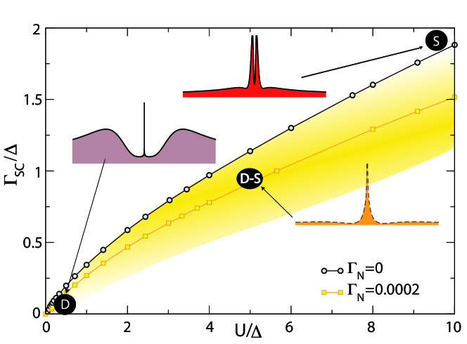
Figure 2: (Color online) Phase diagram for fixed $U=0.01$ and typical spectra for doublet (D), singlet (S) and doublet-singlet cross-over (DS) regimes. Shading indicates the estimated width of the cross-over region.

Since we are aiming at an accurate non-perturbative study of the problem, we adopt the NRG method Wilson2 ; Krishna ; Hofstetter ; Bulla . The NRG is essentially an exact diagonalization procedure where the only approximations are the discretization of the continuum of states in the leads, and the truncation of the almost decoupled high-energy excitations at each iteration step; both are controlled and, in principle, accuracies below 1% can be achieved. The calculations become numerically demanding as the number of “channels” (i.e., leads, here one normal and one superconducting) increases and as the symmetry is reduced (here the only remaining symmetry in the presence of the magnetic field is the conservation of the spin projection $S_{z}$). The present problem is at the very boarder of the currently feasible NRG computations. We employ an iterative diagonalization scheme which consists of including a single site from the Wilson chains in each NRG step, alternatively from the superconducting and from the normal-state lead; we have verified that the difference compared to the conventional approach where two sites are included at once is inconsequential (differences of a few percent). Here this approach works very well because the two channels have very asymmetric coupling and are different in nature, thus the alternating site adding does not lead to the breaking of the energy-scale separation that is necessary in the NRG approach. The discretization parameter was $\Lambda=4$ and we typically kept up to 6000 multiplets per NRG iteration. We made use of the spin symmetry: SU(2) in the absence of field, U(1) in its presence. The spectral function is calculated using the full-density matrix algorithm which is the most reliable approach at finite temperatures weichselbaum2007 .

All relevant physical quantities can be extracted from the QD Green’s functions in the Nambu space defined as

$$\hat{G}(t,t^{\prime})=-i\langle\Psi(t)\Psi^{\dagger}(t^{\prime})\rangle,$$ (4)

where $\Psi=(d_{\uparrow}\;d^{\dagger}_{\downarrow})^{T}$. The spectral function $A(\omega)$ is defined as

$$A(\omega)=-\frac{1}{\pi}\mathrm{Im}G^{r}_{dd}(\omega),$$ (5)

where $G^{r}_{dd}(\omega)$ is the Fourier transform of the QD retarded Green’s function, namely

$$G^{r}_{dd}(\omega)=-i\int_{0}^{\infty}\mathrm{d}t\,e^{i\omega t}\langle\{d_{\sigma}(t),d^{\dagger}_{\sigma}(0)\}\rangle.$$ (6)

The doublet-singlet transition can be characterized by the changes in the anomalous spectral function

$$B(\omega)=-\frac{1}{\pi}\mathrm{Im}F^{r}_{dd}(\omega)$$ (7)

of the anomalous component of the propagator

$$F^{r}_{dd}(\omega)=-i\int_{0}^{\infty}\mathrm{d}t\,e^{i\omega t}\langle\{d_{\uparrow}(t),d_{\downarrow}(0)\}\rangle.$$ (8)

For computing spectral functions we performed averaging over $N_{z}=8$ interleaved discretization grids. Since the impurity is coupled to both normal-state and superconducting channels, we performed the broadening using a standard log-Gaussian scheme with $b=0.6$.

III Phase diagram

For $\Gamma_{N}=0$, large $U$ favors a doublet ground state: in the analytically solvable $\Delta\rightarrow\infty$ limit, the doublet phase occurs for $\Gamma_{SC}$ below the line

$$U=2\sqrt{\xi^{2}+\Gamma_{SC}^{2}}.$$ (9)

For finite $\Delta$, the DS transition needs to be computed numerically (black line with circles in Fig. 2). Large $\Delta$ favors a superconducting singlet state, while for smaller $\Delta$ Kondo correlations mediated by quasiparticles above the superconducting gap are also possible and the singlet becomes predominantly of Kondo character as $\Gamma_{SC}$ increases. In this section we discuss how this picture is modified by the presence of the normal-state lead. We describe different criteria for identifying the doublet-singlet cross-over region, the origin of the additional zero-bias anomalies, and provide numerical results for the $\Gamma_{N}$ dependence.

III.1 Phase transition vs. cross-over behavior

For $\Gamma_{N}\neq 0$, Kondo screening leads to a singlet ground state for all parameter values. We emphasise that this is a statement about the true zero-temperature ground state and that the characteristic temperature scale for reaching such a ground state can be exponentially low, thus experimentally irrelevant. In such circumstances, it is more important to understand the properties at intermediate experimentally relevant temperature scales. We find that the sharp DS quantum phase transition for $\Gamma_{N}\to 0$ is replaced at $\Gamma_{N}\neq 0$ by a smooth cross-over between the “singlet” and “doublet regimes” which can be empirically distinguished by analogy with the $\Gamma_{N}=0$ case in several ways:

1. sign of the local pairing term $\langle d_{\uparrow}d_{\downarrow}\rangle$;

2. merging and splitting of Shiba resonances in the regular spectral function $A(\omega)$;

3. peak weights in the anomalous spectral function $B(\omega)$.

These criteria are fully equivalent for $\Gamma_{N}=0$ when the DS transition marks a true discontinuity in all physical properties, but they define three different lines for finite $\Gamma_{N}$ because the cross-over is smooth and extended. The line with squares in Fig. 2 corresponds to criterion a. The width of the cross-over region, indicated by the shading in Fig. 2, roughly indicates the range where the YSR resonances are merged (criterion b, which is experimentally the most relevant). Due to the significant width of the cross-over region even for small $\Gamma_{N}$, the normal-state electrode cannot be considered as a non-perturbing probe.

Further details about the conceptual and technical issues related to defining the position of the cross-over lines are given in Appendix A.

III.2 Origin of the zero bias anomalies

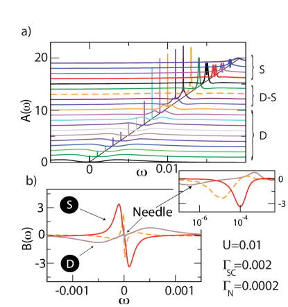
Figure 3: (Color online) a) Spectra for $\Delta$ ranging from $0.5$ (bottom) to $0$ (top). Offsets are added for clarity. b) Anomalous spectral function $B(\omega)$ for $\Delta=0.004$ (doublet), $\Delta=0.002$ (doublet-singlet cross-over, dashed line) and $\Delta=0.001$ (singlet). Inset: $B(\omega)$ for $\omega>0$ on the logarithmic frequency scale. The arrow indicates the peak with negative weight in the doublet regime, which is associated with the Kondo effect and the ultimate spin-singlet ground state.

Spectra exhibit features characteristic for the different regimes and ZBAs of different origins emerge as the gap $\Delta$ decreases, see Fig. 3(a). In the doublet regime, an extremely narrow needle-like Kondo resonance at $\omega=0$ coexists with Shiba resonances at $\omega\neq 0$. The needle is due to the Kondo screening of the magnetic doublet and has a very low Kondo temperature $T_{K}^{N}$ due to small $\Gamma_{N}$. In the DS cross-over region, the Shiba resonances merge with this needle Kondo resonance to produce an enhanced ZBA ($\Delta=0.002$, dashed line) with large height and spectral weight. The maximum weight of this peak corresponds quite accurately to the value of $\Delta$ where $\langle d_{\uparrow}d_{\downarrow}\rangle$ changes sign (criterion a). Decreasing $\Delta$ further, the peak first reduces in amplitude and then splits, signalling the end of the cross-over into the singlet phase, characterized by two Shiba resonances at finite energy. Surprisingly, the splitting happens precisely at the DS transition line of the $\Gamma_{N}=0$ case.

In Fig. 3(b), we plot the anomalous spectral function $B(\omega)$ which provides information about the induced pairing in the quantum dot. For $\Gamma_{N}=0$, inside the gap there would only be delta peaks corresponding to the YSR states with positive weight for $\omega>0$ in the doublet phase, and negative sign in the singlet phase. For finite $\Gamma_{N}$, the YRS delta peaks are broadened into resonances and the DS cross-over corresponds to a transition case featuring both positive and negative spectral weight in $B(\omega)$ for $\omega>0$. Deeper in the doublet phase ($\Delta=0.0004$ case), we observe an important detail: although the anomalous spectral function has predominately positive weight for $\omega>0$, corresponding to an overall doublet character, there is a negative low-weight peak at low frequencies which corresponds to the needle-like ZBA (inset, indicated by an arrow). This small peak allows to rigorously ascribe the needle ZBA to a Kondo singlet ground state. The anomalous spectrum changes sign at the DS point ($\Delta=0.002$, dashed). This sign change can be identified as the point where the integrated weights $\Omega^{\pm}\equiv\int_{0}^{\Delta}d\omega B^{\pm}(\omega)$, with $B^{\pm}(\omega)$ being the positive and negative parts of $B(\omega)$, are equal (criterion c). Beyond this point ($\Delta=0.001$ in the figure), $B(\omega)<0$ for $\omega>0$, as expected for a singlet.

III.3 $\Gamma_{N}$ dependence

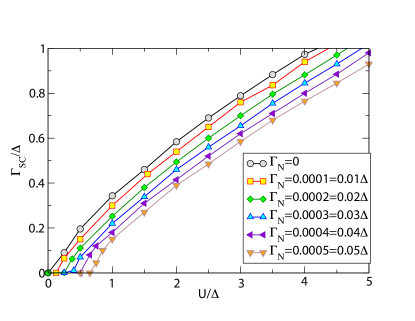
Figure 4: (Color online) Phase diagram (according to the criterion a) for the $DS$ cross-over when $\Gamma_{SC}$ and $U$ are tuned for different values of $\Gamma_{N}$. The gap is fixed to $\Delta=0.01$. Compared to Fig. 2, here $\Delta$ is fixed rather than $U$. For this reason, the behavior near the origin is different. In this figure, the origin corresponds to the non-interacting $U\to 0$ limit, while in Fig. 2 the origin corresponds to the large-gap $\Delta\to\infty$ limit.

To better understand the role of $\Gamma_{N}$, we summarize the results of comprehensive calculations in Fig. 4 where we distinguish the two regimes when both $\Gamma_{SC}$ and $U$ are tuned at fixed $\Delta=0.01$. Even weak coupling to the normal lead has a considerable effect on the phase diagram, the main effect being the significant downward shift (as a function of $\Gamma_{SC}$) of the boundary between the singlet and doublet regimes as $\Gamma_{N}$ increases from zero at a fixed value of $U$. Alternatively, one may study changes in the phase diagram as both $\Gamma_{N}$ and $\Delta$ vary for fixed $U$ and $\Gamma_{SC}$. These results are shown in Fig. 5. Again, small values of $\Gamma_{N}$ (the ranges shown on the vertical axis are always smaller than $\Gamma_{SC}$) can change the phase diagram and induce DS transitions.

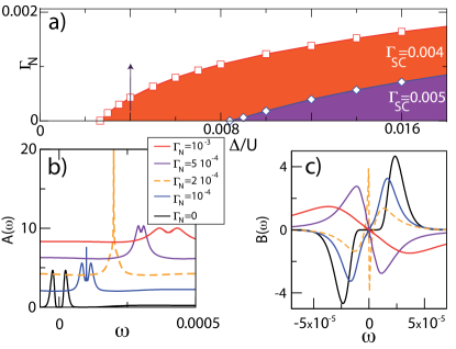
Figure 5: (Color online) a) Phase diagram for fixed $U=0.05$ and two values of $\Gamma_{SC}$ as a function of $\Gamma_{N}$ and $\Delta$. The colored areas denote doublet regions. b) Spectral function (curves offset) and c) anomalous spectrum as we increase $\Gamma_{N}$ along the direction of the arrow in panel a ($\Delta=0.0002$ and $\Gamma_{SC}=0.004$).

The effect of $\Gamma_{N}$ on the width of spectral features–and consequently on the extent of the cross-over region–is presented also in Fig. 6 through the $\Gamma_{SC}$ dependence of the spectral function computed for a range of couplings to the normal-state lead $\Gamma_{N}$. The plots very graphically demonstrate the broadening effect of finite $\Gamma_{N}$. While in the $\Gamma_{N}\to 0$ limit, the crossing of the doublet and singlet states at $\omega=0$ is a discrete event that occurs at a well-defined value of $\Gamma_{SC}$, for non-zero $\Gamma_{N}$ we see that there is an extended range of $\Gamma_{SC}$ for which an observable resonance is pinned at the Fermi level. This range corresponds to the extent of the DS cross-over, indicated in Fig. 2 by shading.

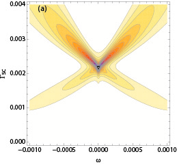
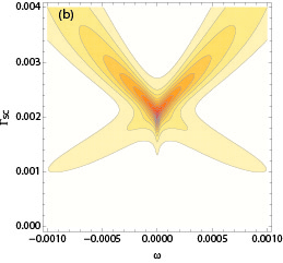
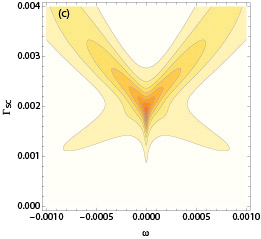
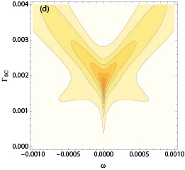
Figure 6: (Color online) Impurity spectral function $A(\omega)$ vs. coupling to the superconducting lead $\Gamma_{SC}$. Calculations are performed at fixed $U=0.01$ and $U/\Delta=5$, and plotted for a range of increasing coupling to the normal-state lead $\Gamma_{N}$: (a) $\Gamma_{N}$=0.0001, (b) $\Gamma_{N}$=0.0002, (c) $\Gamma_{N}$=0.0003 and (d) $\Gamma_{N}$=0.0004. Note the progressively wide range of $\Gamma_{SC}$ where a zero-bias resonance exsits as $\Gamma_{N}$ increases.

III.4 Strong Coulomb interaction regime

In the strong Coulomb interaction regime with large $U/\Delta$ ratio, one can reduce the gap to very small values before crossing over to the singlet ground state. The phase diagram in this regime, shown in Fig. 5 for two fixed values of $\Gamma_{SC}$, demonstrates the role of $\Gamma_{N}$: an increasing $\Gamma_{N}$ can drive a DS crossover (see also panels b and c) which, for the chosen parameter set, occurs at $\Gamma_{N}\approx 2\times 10^{-4}=5\times 10^{-2}\Gamma_{SC}$. For large $U$, the spectra are quite different from the ones shown in Fig. 2. Starting from a typical configuration with a needle (Fig. 7(a), bottom curves), the spectral function evolves for decreasing gap into a characteristic shape which, apart from the needle Kondo peak, has two large Coulomb blockade peaks, two BCS gap-edge singularities, and two emerging Shiba satellites (top curve). Despite the significant changes in the overall shape for varying $\Delta$, these spectra all belong to the doublet regime.

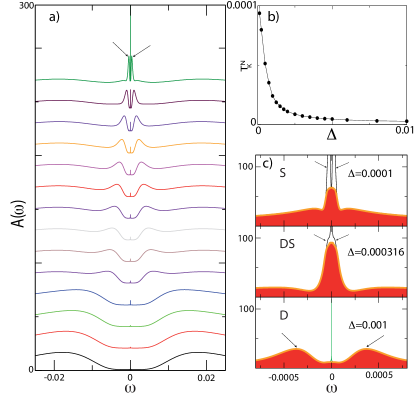
Figure 7: (Color online) Large $U$ case, $U=0.05$. a) Spectral densities for decreasing $\Delta$ (curves offset) from $\Delta=0.05$ (bottom) to $\Delta=0.001$ (top). Other parameters: $\Gamma_{SC}=0.004$, $\Gamma_{N}=0.0004$. b) $T_{K}^{N}$ versus $\Delta$ for the same parameters. c) Spectral functions at finite temperature $T=0.002U$ (shaded curves) as the gap decreases (for a typical charging energy of $U\sim 1\,\mathrm{meV}$, the temperature used in the calculations would correspond to $T\sim 2\,\mathrm{\mu eV}\sim 23\,\mathrm{mK}$). The corresponding zero-temperature results are shown as thin lines.

IV Role of finite temperatures

The role of finite $T$ is most pronounced in the doublet regime. The Kondo temperature of the needle peak, $T_{K}^{N}$, depends exponentially on $\Gamma_{N}$, but not in the standard way since $U$ is renormalized by the screening from the superconducting lead (see Appendix C). Importantly, $T_{K}^{N}$ grows as $\Delta$ decreases, as indicated by the numerical results in Fig. 7(b) and by the Schrieffer-Wolff transformation which shows an enhanced Kondo exchange coupling as $\Delta$ is reduced, as demonstrated in Appendix B. In the large-$U$ regime, this temperature scale may be of the order or larger than the splitting of YRS states after the DS transition. This results in large ZBAs as the gap closes, see Fig. 7(c). Similar features in the spectrum could be attributed to emergent MBS Das12ZBA ; Deng12 ; Finck:PRL13 . Therefore, a word of caution about this interpretation is in order.

V Role of magnetic fields

V.1 Field-induced zero-bias anomaly

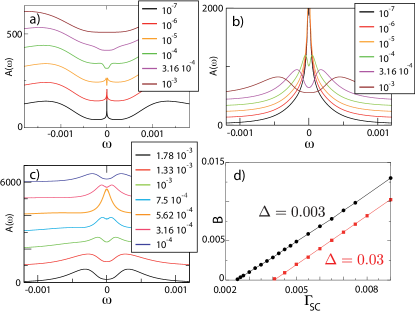
Figure 8: (Color online) Effect of the magnetic field on the spectral functions. We plot the spin-averaged spectral function for a range of magnetic fields $B$ in a) doublet ($\Gamma_{SC}=0.001$), b) DS crossover ($\Gamma_{SC}=0.00225$), and c) singlet ($\Gamma_{SC}=0.003$) regimes (curves vertically offset for clarity). Other parameters are $U=0.01$, $\Gamma_{N}=0.0002$, $\Delta=0.003$. d) Position of the parity crossing in magnetic field versus $\Gamma_{SC}$.

Magnetic field is used to induce topologically nontrivial phases with Majorana states in nanowires; hence it is interesting to see whether ZBAs can be generated by the field also in the quantum dot system. The spectra for a range of fields are presented in Fig. 8. In the doublet regime (panel a), we observe outward shift of the Shiba states induced by enlarged DS excitation energy as $B$ is increased, as well as the Zeeman splitting of the needle ZBA leading to a pronounced dip structure at moderate $B$. In the DS cross-over regime (panel b) where the Kondo peak is already merged with Shiba states, we see the splitting of this collective ZBA. The most interesting case is the S regime (panel c), where parity crossings occur as one of the Zeeman split doublet states becomes the new ground state at some finite $B$: at this point a sizeable ZBA is formed, in agreement with the experiments of Ref. [Lee14, ]. We note that the combined action of the above phenomenology with the previously discussed DS transitions as one reduces the gap would lead to ZBAs that split and re-form, similar to the observations in e.g. Ref. [Finck:PRL13, ].

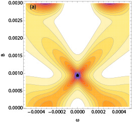
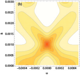
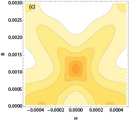
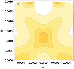
Figure 9: (Color online) Impurity spectral function $A(\omega)$ as a function of the magnetic field $B$. The calculations are performed at fixed $U=0.01$, $\Gamma_{SC}=0.003$, $\Delta/U=0.3$, and plotted for a range of increasing coupling to the normal-state lead $\Gamma_{N}$: (a) $\Gamma_{N}$=0.0001, (b) $\Gamma_{N}$=0.0002, (c) $\Gamma_{N}$=0.0003 and (d) $\Gamma_{N}$=0.0004. Note that $\Gamma_{N}\ll\Gamma_{SC}$ for all cases considered.

In Fig. 9 we plot the dependence of the spectral function on the external magnetic field for a range of hybridization strengths to the normal-state lead, $\Gamma_{N}$. For small $\Gamma_{N}$, the crossing of the lower doublet state with the single YSR state is characterized by a very pronounced zero-bias anomaly occuring at a well defined value of the magnetic field. As $\Gamma_{N}$ increases, the spectral features become more diffuse, thus there is an extended range of magnetic fields with enhanced spectral densities near the Fermi level. This is similar to the behavior observed in some experiments aiming at the detection of Majorana bound states.

V.2 Linear $B$ vs. $\Gamma_{SC}$ dependence

The Zeeman-induced ZBA in the singlet regime is continuously connected with the DS crossing at $B=0$ for a different value of $\Gamma_{SC}$. In fact, our numerical results show that the position in B field of this ZBA depends linearly on $\Gamma_{SC}$ for any value of $\Delta$ (Fig. 8(d)). This is highly surprising, since the singlet-doublet splitting is non-linear in $\Gamma_{SC}$, and the Zeeman splitting is non-linear in both $\Gamma_{SC}$ and $B$; nevertheless, the intersection happens along a straight line in the $(B,\Gamma_{SC})$ plane as long as the system is particle-hole symmetric.

This linear dependence can be obtained analytically in the small $\Gamma_{N}$ limit by studying the conditions for the occurence of the subgap states exactly at the Fermi level at $\omega=0$. We will thus focus on the $|\omega|\ll\Delta$ limit, noting that this is not at all the same as the $\Delta\to\infty$ limit. We assume that the magnetic field is applied along the $z$ axis.

The interaction effects are fully described by the self-energy matrix, introduced through the Dyson equation

$$\hat{G}(z)^{-1}=\hat{G}^{(0)}(z)^{-1}-\hat{\Sigma}(z),$$ (10)

where the non-interacting Green’s function matrix is

$$\hat{G}^{(0)}(z)^{-1}=z-\epsilon\tau_{3}-E_{Z}\sigma_{3}-V^{2}\tau_{3}\frac{1}{N}\sum_{k}g_{k}(z)\tau_{3}.$$ (11)

Here $z$ is the complex frequency argument (taken to be $z=\omega+i\delta$ at the end of the calculation to obtain the retarded Green’s functions), $E_{Z}=g\mu_{B}B/2$ is the Zeeman energy, $V$ is the coupling to the superconducting lead (the normal lead is not considered in this section), $N$ is the number of $k$ states in the lead, $g_{k}(z)$ is the Green’s function for an electron in the superconducting lead and, finally, $\tau_{i}$ are Pauli matrices in the Nambu (particle-hole) space, while $\sigma_{i}$ are Pauli matrices in the spin space. For magnetic field applied along the $z$ axis, it is possible to work either with the $2\times 2$ Nambu structure with $\Psi=(d_{\uparrow}d_{\downarrow}^{\dagger})^{T}$, or with the $4\times 4$ Nambu structure with $\Psi=(d_{\uparrow}d_{\downarrow}d_{\downarrow}^{\dagger}d_{\uparrow}^{\dagger})^{T}$. In the latter case, the $2\times 2$ submatrices are actually diagonal. In the former case, the $\sigma_{3}$ matrix in Eq. (11) needs to be replaced by the identity.

Since

$$g_{k}(z)^{-1}=z-\epsilon_{k}\tau_{3}+\Delta\tau_{1}\sigma_{3},$$ (12)

one finds

$$g_{k}(z)=\frac{z+\epsilon_{k}\tau_{3}-\Delta\tau_{1}\sigma_{3}}{z^{2}-(\epsilon_{k}^{2}+\Delta^{2})}.$$ (13)

Summing over $k$ in Eq. (11), one obtains

$$G^{(0)}(z)^{-1}=z-\epsilon\tau_{3}-E_{Z}\sigma_{3}+\Gamma_{SC}\frac{(z+\Delta\tau_{1}\sigma_{3})}{E(z)},$$ (14)

where the last term is the self-energy originating from the coupling with the superconducting lead. $E(z)$ can be analytically continued to $E(\omega)=\sqrt{\Delta^{2}-\omega^{2}}$. In the $\omega\to 0$ limit, $E(0)=\Delta$ and the coupling self-energy reduces to $\Gamma_{SC}\tau_{1}\sigma_{3}$. Note that in this limit the gap $\Delta$ disappears from the problem such that $\Gamma_{SC}$ plays the role of an effective pairing term.

The Shiba states are identified as the poles of the Green’s function inside the gap:

$$\text{det}[G^{-1}(z)]=0,$$ (15)

where $z$ needs to be on the real axis for a true bound state, while resonances correspond to true solutions with a small imaginary component (this would be the case for $\Gamma_{N}\neq 0$).

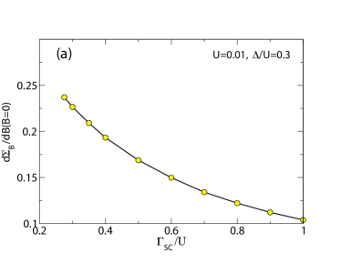
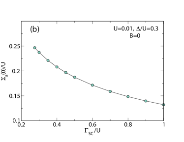
Figure 10: (Color online) (a) Slope of the real part of $\Sigma_{B}(B)$ self-energy function. This quantity can be interpreted as the renormalization of the effective $g$-factor due to interactions. (b) Zero-frequency value of the real part of the anomalous self-energy, $\mathrm{Re}\Sigma_{a}(\omega=0)$ in the singlet regime, $\Gamma>\Gamma_{DS}$.

In the absence of interactions, the condition for a sub-gap state takes the following form:

$$z^{2}-\epsilon^{2}-E_{Z}z+E_{Z}^{2}-\Gamma_{SC}^{2}\frac{\Delta^{2}-z^{2}}{E(z)^{2}}+\frac{2z(z-E_{Z})\Gamma_{SC}}{E(z)}=0.$$ (16)

Taking the $|z|\ll\Delta$ limit, this yields

$$E_{Z}^{2}=\Gamma_{SC}^{2}+\epsilon^{2}.$$ (17)

Interestingly, this condition for a Zeeman-induced zero-energy YSR state in a non-interacting quantum dot is the same as the one in Eq. (2) for obtaining the MBS in a nanowire (as we mentioned, in the $z\rightarrow 0$ limit $\Gamma_{SC}$ plays the role of an effective pairing term $\Delta_{*}$, while $\epsilon$ plays the role of a chemical potential in the quantum dot).

Eq. (17) can be easily generalized to the interacting case. The structure of the self-energy matrix is

$$\hat{\Sigma}(z)=\begin{pmatrix}\Sigma_{\uparrow}(z)&0&\Sigma_{a}(z)&0\\ 0&\Sigma_{\downarrow}(z)&0&-\Sigma_{a}(-z)\\ \Sigma_{a}(z)&0&-\Sigma_{\downarrow}(-z)&0\\ 0&-\Sigma_{a}(-z)&0&-\Sigma_{\uparrow}(-z)\end{pmatrix},$$ (18)

where $\Sigma_{\sigma}(z)$ are the regular self-energy components, while $\Sigma_{a}(z)$ is the anomalous component. To study the positions of the sub-gap peaks, a low-order expansion can be performed:

$$\hat{\Sigma}(z)=\hat{\Sigma}(0)+\hat{\Sigma}^{\prime}(0)z=\hat{\Sigma}(0)+(1-\hat{Z}^{-1})z,$$ (19)

where $\hat{Z}$ is the (matrix-valued) quasiparticle renormalization factor $\hat{Z}^{-1}=1-\hat{\Sigma}^{\prime}(0)$ whose deviation from the identity matrix quantifies the strength of the interaction effects. In fact, for our consideration of the zero-crossing, we truncate the expansion at the first term. This is an important observation which holds in general: the condition for the zero-energy Shiba state does not depend explicitly on the quasiparticle renormalization factor (i.e., on the Kondo temperature). We are thus only interested in the zero-frequency values, $\hat{\Sigma}(0)$. These are purely real, since the self-energy has zero imaginary part inside the superconducting gap. We insert the self-energy matrix in Eq. (11), evaluate the determinant in the $|\omega|\ll\Delta$ limit, and after some lengthy algebra obtain the following expression:

$$(E_{Z}+\Sigma_{B})^{2}=(\Gamma_{SC}-\Sigma_{a})^{2}+(\epsilon+\Sigma_{0})^{2},$$ (20)

where we have introduced the spin-averaged normal self-energy $\Sigma_{0}\equiv\frac{1}{2}(\Sigma_{\uparrow}(0)+\Sigma_{\downarrow}(0))$ and the spin component $\Sigma_{B}\equiv\frac{1}{2}(\Sigma_{\uparrow}(0)-\Sigma_{\downarrow}(0))$, with $\Sigma_{\sigma}(0)=Un_{\bar{\sigma}}$. This equation maintains the structure of Eq. (17), the only new effects are the interaction-induced shifts. In the particle-hole symmetric case, one has $\Sigma_{0}=U/2$ and $\epsilon=-U/2$, thus the last term drops out. Then

$$E_{Z}+\Sigma_{B}=\Gamma_{SC}-\Sigma_{a}.$$ (21)

This equation turns out to describe a linear relation between $E_{Z}$ (i.e., field $B$) and $\Gamma_{SC}$ despite the non-trivial $\Gamma_{SC}$-dependence of the self-energies $\Sigma_{B}$ and $\Sigma_{a}$, since $\Sigma_{B}$ is proportional to $B$ to a very good approximation, $\Sigma_{B}=c(\Gamma_{SC})B$, and there appears to be a connection between the Fermi-level derivative of the spin-dependent self-energy $c(\Gamma_{SC})=\mathrm{d}\Sigma_{B}/\mathrm{d}B|_{\omega=0}$ and the anomalous self-energy $\Sigma_{a}(\Gamma_{SC})$, see Figs. 10(a) and 10(b). Plotting $(\Gamma-\Sigma_{a}(\Gamma))/(1+\mathrm{d}\Sigma_{B}/\mathrm{d}B)$ as a function of $\Gamma$, one obtains a straight line with a slope close to 2.

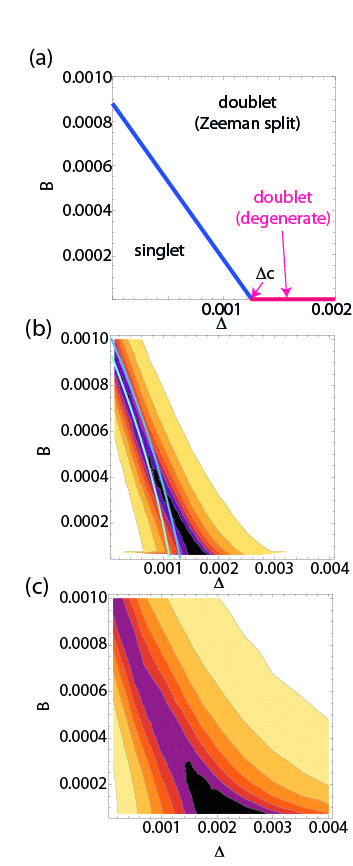
Figure 11: (Color online) (a) Phase diagram in the $(B,\Delta)$ plane for $\Gamma_{N}=0$. At $\Delta_{c}\sim 0.0012$, the ground state of the system at $B=0$ changes from singlet to doublet. (b,c) Zero-frequency spectral function $A(\omega=0)$ plotted as a function of the gap $\Delta$ and the external magnetic field $B$, revealing the behavior of the zero-bias anomaly in the $(\Delta,B)$ plane. The coupling to the normal-state lead is (b) $\Gamma_{N}=0.0002$, and (c) $\Gamma_{N}=0.0004$. In (b) we also plot (in blue) two possible lines for the evolution of the gap for increasing magnetic fields. We use the function $\Delta(B)\sim\Delta[1-0.32B-0.1B^{2}]$, based on a fitting of the experimental data from Ref. [Lee14, ]. Both curves correspond to gap values $\Delta=0.0011$ and $0.0013$, respectively, which are located on either side of the $\Gamma_{N}=0$ transition around $\Delta_{c}$. Rest of parameters: $\Gamma_{SC}=0.002$ and $U=0.01$.

We also note that for zero-field, the DS cross-over is defined through

$$\Gamma_{SC}=\Sigma_{a}(\Gamma_{SC}).$$ (22)

We conclude that the ZBA occurs for

$$\tilde{E}_{Z}^{2}=\tilde{\Gamma}_{SC}^{2}+\tilde{\epsilon}^{2}.$$ (23)

Here, tilde quantities represent parameters renormalized by interactions $X\rightarrow\tilde{X}\equiv X+Re\Sigma(\omega=0)$. At the particle-hole symmetric point the last term drops out so that

$$\pm\tilde{E}_{Z}=\tilde{\Gamma}_{SC}.$$ (24)

We stress again that this linear relation for arbitrary $U$ and $\Delta$ is remarkable since the corresponding self-energies renormalizing the bare parameters, like for instance the renormalized g-factor that can be extracted from $\tilde{E}_{Z}$, are themselves non-linear functions of $\Gamma_{SC}$.

Interestingly, Eq. (23) still has the same structure as Eq. (17). Therefore, the general condition for Zeeman-induced parity crossings of YSR bound states, fully taking into account interactions, and the condition for reaching a topological phase in a non-interacting nanowire (Eq. (2)) are still analogous.

V.3 Zero-bias anomalies studied in the $(\Delta,B)$ plane

In experiments performed on nanowires exposed to external magnetic field, the role of the field is two-fold: (a) it leads to Zeeman splitting of the doublet YSR states, and (b) it suppresses the BCS pairing parameter $\Delta$. Up to now, we have presented results computed for varying $B$ at fixed $\Delta$. For completeness, we now provide some results computed as a function of both $B$ and $\Delta$: the actual experimental situation corresponds to some $\Delta=\Delta(B)$ curve in this plane.

In Fig. 11(a) we present the phase diagram in the $\Gamma_{N}\to 0$ limit. For small $\Delta$, the ground state at zero field is a singlet. As $B$ increases, one of the Zeeman-split doublet levels is brought down in energy and eventually becomes the new ground state. In this part of the diagram, we observe linear dependence between $\Delta$ and $B$ at the doublet-singlet transition. Note that this is yet another unexpected linearity, different (but related) to the one in the $(\Gamma_{SC},B)$ plane discussed above.

The effect of the coupling to the normal-state leads is demonstrated in Fig. 11(b,c), where we plot the dependence of the spectral function at zero frequency, $A(0)$, on $\Delta$ and $B$. The spectra are strongly enhanced (i.e., feature a zero-bias anomaly) in two regions: (i) for small $\Delta<\Delta_{c}\approx 0.0012$ for magnetic fields where the singlet and doublet states cross at $\omega=0$, and (ii) for large $\Delta>\Delta_{c}$ near zero-field, due to the needle-like Kondo resonance induced directly by the normal-state tunneling probe. We note that in this case non-zero $\Gamma_{N}$ strongly suppresses the linearity of the ZBA in region (i).

The precise $\Delta(B)$ function form depends on the experimental details. To indicate the possible behavior, we overlayed two curves on Fig. 11(b,c). Both curves, based on realistic $\Delta(B)$ dependence for the particular experiment described in Ref. Lee14, , indicate that persisting ZBAs can be found in this parameter plane. Both curves correspond to gap values, at $B=0$, around $\Delta_{c}$. The lighter curve corresponds to the case where upon increasing $B$, the ZBA appears and persists practically until the gap closure. The darker curve corresponds to the case where the ZBA first appears and then splits again before the gap is ultimately closed.

VI Conclusion

We have calculated the phase diagram of an Anderson impurity in contact with superconducting and normal-state leads by means of the numerical renormalization group, and established that even a very weak coupling to the normal lead perturbs the system. Our results, valid for an arbitrary ratio $\Delta\over T_{K}$, are analyzed in the context of experimental scenarios such as zero-bias anomalies induced by parity crossing transitions of Yu-Shiba-Rusinov bound states and novel Kondo features induced by the normal lead. In particular, we have discussed how spectral functions at finite temperatures and magnetic fields, which can be directly linked to experimental tunneling transport characteristics, can show zero-energy anomalies irrespective of whether the system is in the doublet or singlet regime. These results indicate that due caution is needed in interpreting experiments aiming to detect Majorana bound states since in hybrid systems Kondo physics and parity crossings may manifest in unanticipated ways.

We have also derived the analytical condition for the occurrence of Zeeman-induced fermion-parity switches in the presence of interactions, Eq. (23), which bears unexpected similarities with the condition for emergent Majorana bound states in nanowires, Eq. (2). This result suggests that the physics of Zeeman-induced parity-crossings in the minimal Anderson model in contact with a superconductor is connected with the condition for emergent Majorana bound states. This similarity thus leads to an interesting question: Is this equivalence between Eq. (2) and Eq. (23) general? While we do not have a final answer for this, we note that the analogy persists for finite spin-orbit coupling in the non-interacting regime: it has been shown Stanescu:PRB13 that Zeeman-induced parity crossings in short non-interacting nanowires (with finite spin-orbit coupling) smoothly evolve towards true topological transitions as the wire becomes longer. Whether our interacting results are also smoothly connected with MBS physics in the finite spin-orbit case and beyond the single quantum impurity limit remains an open question worth to be investigated.

Appendix A Doublet-singlet transition induced by the normal-state lead

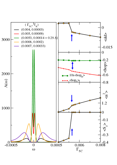
Figure 12: (Color online) Left panel: Impurity spectral functions for a range of hybridization strengths to the superconducting lead ($U=0.05$ and $\Delta/U=0.01$). Normal lead is nearly decoupled. The doublet-singlet transition occurs for $\Delta=3.6T_{K}$ or $T_{K}=0.3\Delta$, where $T_{K}$ is Wilson’s Kondo temperature. Right panel: Expectation values as a function of $\Gamma_{SC}$. All the criteria show a DS transition at $\Gamma_{SC}\approx 5.3\times 10^{-3}$ (arrows).

To better illustrate how the doublet-singlet (DS) transition occurs, we consider a situation in which the superconducting coupling $\Gamma_{SC}$ increases while the normal-lead coupling is fixed to a very small value $\Gamma_{N}=10^{-5}$ (effectively zero). Due to the smallness of $\Gamma_{N}$, this situation can be identified with an effective SC-QD setup. We plot in Fig. 12(a) the impurity spectral function when $U=0.05$, at a fixed superconductig gap value $\Delta/U=0.01$. In order to clearly identify the doublet regions, we include small but finite temperature and magnetic field. Finite $B$ field leads to a sizeable non-zero magnetization sufficiently deep in the doublet phase because the magnetic moment remains unscreend; the magnetization starts to increase at the DS transition. Also, because $T$ is finite, one may indeed characterize the small-$\Gamma_{SC}$ phase as the doublet phase (in the zero-temperature limit, the ground state is strictly speaking a singlet for any non-zero $\Gamma_{N}$). The impurity spectral function shows the DS transition when $\Gamma_{SC}\approx 5.3\times 10^{-3}$, which, as expected, corresponds to $T_{K}\approx 0.3\Delta$.

More rigorously, one may locate the DS transition point by employing several criteria based on the behavior of: (i) the pairing term $\langle d_{\uparrow}d_{\downarrow}\rangle$, (ii) the hopping functions $h_{\alpha}=\sum_{\sigma}\langle d_{\sigma}^{\dagger}f_{0\sigma\alpha}+\text{H.c.}\rangle$, where $f_{0\sigma\alpha}$ is the combination of the conduction band orbitals to which the impurity couples, (iii) charge fluctuations $\langle n^{2}\rangle$ (with $n=\sum_{\sigma}d_{\sigma}^{\dagger}d_{\sigma}$ as the total impurity occupation), and finally (iv) $S_{z}=1/2(n_{\uparrow}-n_{\downarrow})$ (the $z$ component of the impurity spin, i.e., the magnetization). All these quantities are displayed in Fig. 12(b) and show a transition at $\Gamma_{SC}\approx 5.3\times 10^{-3}$ (arrows), where all these quantities are discontinuous. In particular, $\langle d_{\uparrow}d_{\downarrow}\rangle$ changes sign, while $\langle S_{z}\rangle$ becomes large in the doublet phase (being essentially zero in the single phase) due to the weak but non-zero external magnetic field.

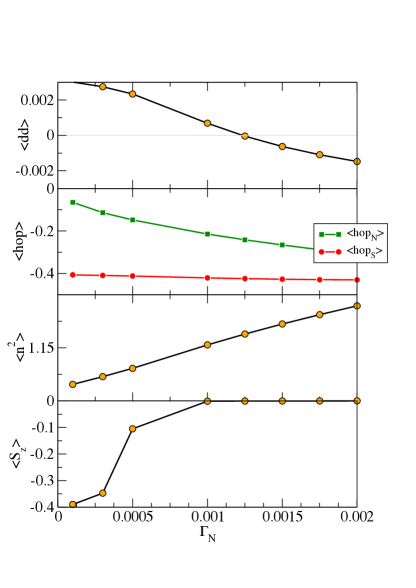
Figure 13: (Color online) Expectation values as a function of $\Gamma_{N}$ for a fixed $\Gamma_{SC}=0.004$ (the rest of parameters are the same as in Fig. 12). The pairing term (top panel) changes sign at $\Gamma_{N}\approx 1.25\times 10^{-3}$ whereas the magnetization (bottom panel) is non-zero for a slightly smaller value $\Gamma_{N}=10^{-3}$.

Now that we have established clear criteria for the DS transition, we study how the above quantities vary as we increase $\Gamma_{N}$ for a fixed $\Gamma_{SC}=0.004$ (Fig. 13). As argued above, different criteria define different values of $\Gamma_{N}$ at which the system crosses over from doublet to singlet regime. Here, for instance, the pairing term (top panel) changes sign at $\Gamma_{N}=1.25\times 10^{-3}$ while the magnetization (bottom panel) is non-zero already at $\Gamma_{N}=10^{-3}$. These different values of $\Gamma_{N}$ according to the different criteria define a sizable cross-over region in the phase diagram.

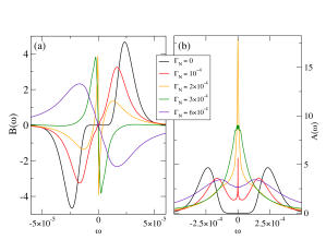
Figure 14: (Color online). (a) Characterization of the singlet phase by the anomalous spectral function $B(\omega)$ for a range of $\Gamma_{N}$. (b) Spectral function $A(\omega)$. The model parameters are $U=0.05$, $\Gamma_{SC}=0.004$, $\Delta=0.0002$.

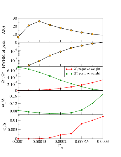
Figure 15: (Color online). From top to bottom: zero-bias peak in the spectral function $A(0)$, width of the peak at zero frequency, $\Omega^{\pm}\equiv\int_{0}^{\Delta}d\omega B^{\pm}(\omega)$ (with $B^{\pm}(\omega)$ being the positive and negative parts of $B(\omega)$), and positive and negative peak positions of $B(\omega)$.

One can also monitor the DS crossover via the anomalous spectral function, as the peak position changes from positive to negative side, indicating the occurence of the crossover. In Fig. 14(a) we have plotted the anomalous spectral function $B(\omega)$ when $\Gamma_{N}$ is varied for a fixed value of $\Gamma_{SC}=0.004$, and $U=0.05$ with $\Delta=2\times 10^{-4}$. For completeness we also provide in Fig. 14(b) the regular spectral function that has a pronounced $\omega=0$ peak precisely when the anomalous spectral function reverses sign. We note especially the case for $\Gamma_{N}=2\times 10^{-4}$ [orange curve in Fig. 14(a)]. The anomalous spectral function $B(\omega)$ has a complex behavior: there is one positive peak at $\omega>0$, just like in the doublet regime, but also one negative peak for $\omega>0$ (close to $\omega=0$), just like in the singlet regime, so this is truly where the crossover between the doublet and singlet regimes can be located. Note, however, that there are numerous possible ways to define the “crossover value” of $\Gamma_{N}$: zero-frequency spectral weight $A(0)$, crossing point of the integrated weights of the anomalous spectral function $W_{+}$ and $W_{-}$, or through peaks positions in $B(\omega)$. The alternative crossover values for $\Gamma_{N}$ attending to the previous criteria are illustrated in Fig. 15: the curves do not define a unique special $\Gamma_{N}$ point.

We note that for $\Gamma_{N}=0$, the DS transition curve is determined by the well-known $T_{K}=0.3\Delta$ rule, where $T_{K}$ is the Kondo temperature according to Wilson’s definition, calculated for the SC lead when the superconductivity is suppressed ($\Delta\to 0$) limit. A relevant question is whether this rule still holds for $\Gamma_{N}\neq 0$ with $T_{K}$ computed for $\Gamma_{\mathrm{eff}}=\Gamma_{N}+\Gamma_{SC}$. We find that this produces the shift of the cross-over line in the correct direction (toward smaller $\Gamma_{SC}$; see Figs. 2 and 4), although quantitatively we find that the effect of finite $\Gamma_{N}$ is more complex.

Appendix B The Schrieffer-Wolff transformation for a NS-impurity system

We perform here the Schrieffer-Wolff transformation Schrieffer66 for the NS-impurity system. By doing this we obtain the exchange couplings for the impurity spin-flip processes from which a functional form for the Kondo temperature can be inferred. Our starting point is a hybrid normal-superconductor Anderson Hamiltonian

$${\cal{H}}={\cal{H}}_{N}+{\cal{H}}_{S}+{\cal{H}}_{D}+{\cal{H}}_{T}={\cal{H}}_{0}+{\cal{H}}_{T}\,,$$ (25)

where

$${\cal{H}}_{N} =\sum_{k,\sigma}\epsilon_{k_{N}}c_{k_{N}\sigma}^{\dagger}c_{k_{N}\sigma}\,,$$ (26a)

$${\cal{H}}_{S} =\sum_{k,\sigma}\epsilon_{k_{SC}}c_{k_{SC}\sigma}^{\dagger}c_{k_{SC}\sigma}+\sum_{k}\left(\Delta c_{k_{SC}\uparrow}^{\dagger}c_{\bar{k}_{SC}\downarrow}^{\dagger}+\text{H.c.}\right)\,,$$ (26b)

$${\cal{H}}_{D} =\sum_{\sigma}\epsilon_{d\sigma}d_{\sigma}^{\dagger}d_{\sigma}+Un_{d\uparrow}n_{d\downarrow}\,,$$ (26c)

$${\cal{H}}_{T} =\sum_{\alpha,k,\sigma}\left(V_{\alpha}c_{k_{\alpha}\sigma}^{\dagger}d_{\sigma}+\text{H.c.}\right)\,.$$ (26d)

The operator $c_{k_{\alpha}\sigma}$ ($c_{k_{\alpha}\sigma}^{\dagger}$) annihilates (creates) an electron with wave-vector $k$ ($\bar{k}=-k$), energy $\epsilon_{k_{\alpha}}$ and spin $\sigma=\{\uparrow,\downarrow\}$ in the normal or superconducting lead ($\alpha=\{N,SC\}$). Similarly, $d_{\sigma}$ ($d_{\sigma}^{\dagger}$) destroys (creates) an electron with spin $\sigma$ and energy $\epsilon_{d\sigma}$ at the impurity level. $n_{d\sigma}=d_{\sigma}^{\dagger}d_{\sigma}$ is the impurity occupation and $U$ denotes the on-site Coulomb interaction. Tunneling amplitudes for normal-impurity and superconducting-impurity processes are indicated by $V_{N}$, and $V_{S}$, respectively. Here, $\Delta$ denotes the superconducting gap considered to be real.

It is convenient to introduce the Bogoliubov-Valatin transformation Bogoliubov58A ; Bogoliubov58B ; Valatin58

$$\begin{pmatrix}c_{k_{SC}\uparrow}\\ c_{\bar{k}_{SC}\downarrow}^{\dagger}\end{pmatrix}=\begin{pmatrix}u_{k}&-v_{k}\\ v_{k}&u_{k}\end{pmatrix}\begin{pmatrix}a_{k}\\ b_{\bar{k}}^{\dagger}\end{pmatrix}\,.$$ (27)

The superconducting coherence factors satisfy the relations

$$u_{k}^{2}=\frac{1}{2}\left(1+\frac{\epsilon_{k_{SC}}}{E_{k}}\right),\,\,v_{k}^{2}=\frac{1}{2}\left(1-\frac{\epsilon_{k_{SC}}}{E_{k}}\right)$$ (28)

with $E_{k}=\sqrt{\epsilon_{k_{SC}}^{2}+\Delta^{2}}$. $u_{k}=u_{\bar{k}}$, $v_{k}=v_{\bar{k}}$, and $E_{k}=E_{\bar{k}}$ are obeyed. Using the transformation, ${\cal{H}}_{S}$ becomes

$${\cal{H}}_{S}=\sum_{k}E_{k}(a_{k}^{\dagger}a_{k}+b_{k}^{\dagger}b_{k})\,,$$ (29)

while ${\cal{H}}_{T}$ is expressed in the form

$${\cal{H}}_{T}=\sum_{k}\left\{V_{S}\left[\left(u_{k}a_{k}^{\dagger}-v_{k}b_{\bar{k}}\right)d_{\uparrow}+\left(v_{k}a_{k}+u_{k}b_{\bar{k}}^{\dagger}\right)d_{\downarrow}\right]\right.\\ \left.+V_{S}\left[d_{\uparrow}^{\dagger}\left(u_{k}a_{k}-v_{k}b_{\bar{k}}^{\dagger}\right)+d_{\downarrow}^{\dagger}\left(v_{k}a_{k}^{\dagger}+u_{k}b_{\bar{k}}\right)\right]\right\}\\ +\sum_{k,\sigma}V_{N}\left(c_{k_{N}\sigma}^{\dagger}d_{\sigma}+d_{\sigma}^{\dagger}c_{k_{N}\sigma}\right)\,.$$ (30)

We make an unitary transformation to get an effective Hamiltonian

$${\cal{H}}_{eff}=e^{S}{\cal{H}}e^{-S}=\sum_{n=0}^{\infty}\frac{1}{n!}[S,{\cal{H}}]_{n}\approx\\ {\cal{H}}_{0}+{\cal{H}}_{T}+[S,{\cal{H}}_{0}]+[S,{\cal{H}}_{T}]+\frac{1}{2!}[S,[S,{\cal{H}}_{0}]]\,,$$ (31)

where $[S,{\cal{H}}]_{0}={\cal{H}}$ and $[S,{\cal{H}}]_{n}=[S,[S,[\cdots,[S,{\cal{H}}]]\cdots]]$. Our purpose is to find an $S$ which satisfies

$${\cal{H}}_{T}+[S,{\cal{H}}_{0}]=0$$ (32)

The effective Hamiltonian then becomes

$${\cal{H}}_{eff}={\cal{H}}_{0}+[S,{\cal{H}}_{T}]+\frac{1}{2!}[S,-{\cal{H}}_{T}]={\cal{H}}_{0}+\frac{1}{2}[S,{\cal{H}}_{T}]\,.$$ (33)

For our setup, the generator $S=S_{0}-S_{0}^{\dagger}$ reads Salomaa88

$$S_{0}=\sum_{k}V_{S}\left\{\left[\frac{n_{d\downarrow}}{E_{k}-\epsilon_{d\uparrow}-U}+\frac{1-n_{d\downarrow}}{E_{k}-\epsilon_{d\uparrow}}\right]u_{k}a_{k}^{\dagger}d_{\uparrow}+\left[\frac{n_{d\downarrow}}{E_{\bar{k}}+\epsilon_{d\uparrow}+U}+\frac{1-n_{d\downarrow}}{E_{\bar{k}}+\epsilon_{d\uparrow}}\right]v_{k}b_{\bar{k}}d_{\uparrow}\right.\\ \left.-\left[\frac{n_{d\uparrow}}{E_{\bar{k}}+\epsilon_{d\downarrow}+U}+\frac{1-n_{d\uparrow}}{E_{\bar{k}}+\epsilon_{d\downarrow}}\right]v_{k}a_{\bar{k}}d_{\downarrow}+\left[\frac{n_{d\uparrow}}{E_{k}-\epsilon_{d\downarrow}-U}+\frac{1-n_{d\uparrow}}{E_{k}-\epsilon_{d\downarrow}}\right]u_{k}b_{k}^{\dagger}d_{\downarrow}\right\}\\ +\sum_{k,\sigma}V_{N}\left[\frac{n_{d\bar{\sigma}}}{\epsilon_{k_{N}}-\epsilon_{d\sigma}-U}+\frac{1-n_{d\bar{\sigma}}}{\epsilon_{k_{N}}-\epsilon_{d\sigma}}\right]c_{k_{N}\sigma}^{\dagger}d_{\sigma}$$ (34)

where $\bar{\sigma}=\downarrow/\uparrow$ for $\sigma=\uparrow/\downarrow$. It is easy to check that the generator $S$ satisfies Eq. (32).

The transformed Hamiltonian can be arranged in a concise form

$${\cal{H}}_{eff}={\cal{H}}_{0}^{\prime}+{\cal{H}}_{PS}+{\cal{H}}_{SF}+{\cal{H}}_{QSF}\,.$$ (35)

Here, ${\cal{H}}_{0}^{\prime}$ corresponds to ${\cal{H}}_{0}$ with renormalized parameters and ${\cal{H}}_{PS}$ denotes the potential scattering of electrons off the impurity. The impurity-electron spin-flip processes are described by

$${\cal{H}}_{SF}=-\frac{1}{2}\sum_{k,p}\sum_{\sigma}J_{N,N,k,p}c_{k_{N}\sigma}^{\dagger}c_{p_{N}\bar{\sigma}}d_{\bar{\sigma}}^{\dagger}d_{\sigma}\\ -\frac{1}{2}\sum_{k,p}\sum_{\sigma}J_{N,S,k,p}c_{k_{N}\sigma}^{\dagger}c_{p_{SC}\bar{\sigma}}d_{\bar{\sigma}}^{\dagger}d_{\sigma}\\ -\frac{1}{2}\sum_{k,p}\sum_{\sigma}J_{S,N,k,p}c_{k_{SC}\sigma}^{\dagger}c_{p_{N}\bar{\sigma}}d_{\bar{\sigma}}^{\dagger}d_{\sigma}\\ -\frac{1}{2}\sum_{k,p}\sum_{\sigma}J_{S,S,k,p}c_{k_{SC}\sigma}^{\dagger}c_{p_{SC}\bar{\sigma}}d_{\bar{\sigma}}^{\dagger}d_{\sigma}\\ +\frac{1}{2}\sum_{\alpha}\sum_{k,p}\sum_{\sigma}{\rm sgn}(\sigma)\left(T_{S,\alpha,k,p}c_{p_{\alpha}\bar{\sigma}}c_{\bar{k}_{SC}\bar{\sigma}}d_{\bar{\sigma}}^{\dagger}d_{\sigma}+\text{H.c.}\right)\,,$$ (36)

where

$$J_{N,N,k,p}=V_{N}^{2}\left[\frac{1}{\epsilon_{k_{N}}-\epsilon_{d}-U}-\frac{1}{\epsilon_{k_{N}}-\epsilon_{d}}\right.\\ \left.+\frac{1}{\epsilon_{p_{N}}-\epsilon_{d}-U}-\frac{1}{\epsilon_{p_{N}}-\epsilon_{d}}\right]\,,$$ (37)

$$J_{N,S,k,p}=J_{S,N,p,k}=V_{N}V_{S}\left[\frac{1}{\epsilon_{k_{N}}-\epsilon_{d}-U}-\frac{1}{\epsilon_{k_{N}}-\epsilon_{d}}\right]\\ +V_{S}V_{N}\Big{[}\frac{u_{p}^{2}}{E_{p}-\epsilon_{d}-U}-\frac{u_{p}^{2}}{E_{p}-\epsilon_{d}}\\ -\frac{v_{p}^{2}}{E_{\bar{p}}+\epsilon_{d}+U}+\frac{v_{p}^{2}}{E_{\bar{p}}+\epsilon_{d}}\Big{]}\,,$$ (38)

$$J_{S,S,k,p}=V_{S}^{2}\Big{[}\frac{u_{k}^{2}}{E_{k}-\epsilon_{d}-U}-\frac{u_{k}^{2}}{E_{k}-\epsilon_{d}}\\ -\frac{v_{k}^{2}}{E_{\bar{k}}+\epsilon_{d}+U}+\frac{v_{k}^{2}}{E_{\bar{k}}+\epsilon_{d}}\\ +\frac{u_{p}^{2}}{E_{p}-\epsilon_{d}-U}-\frac{u_{p}^{2}}{E_{p}-\epsilon_{d}}\\ -\frac{v_{p}^{2}}{E_{\bar{p}}+\epsilon_{d}+U}+\frac{v_{p}^{2}}{E_{\bar{p}}+\epsilon_{d}}\Big{]}\,,$$ (39)

$$T_{S,\alpha,k,p}=V_{S}V_{\alpha}u_{k}v_{k}\Big{[}\frac{1}{E_{k}-\epsilon_{d}-U}-\frac{1}{E_{k}-\epsilon_{d}}\\ +\frac{1}{E_{\bar{k}}+\epsilon_{d}+U}-\frac{1}{E_{\bar{k}}+\epsilon_{d}}\Big{]}\,.$$ (40)

The final term shows the charge-transfer interaction given by

$${\cal{H}}_{QSF}=-\frac{1}{2}\sum_{\alpha}\sum_{k,p}\sum_{\sigma}\left(K_{N,\alpha,k,p}c_{k_{N}\sigma}^{\dagger}c_{p_{\alpha}\bar{\sigma}}^{\dagger}d_{\bar{\sigma}}d_{\sigma}+\text{H.c.}\right)\\ -\frac{1}{2}\sum_{\alpha}\sum_{k,p}\sum_{\sigma}\left(K_{S,\alpha,k,p}c_{k_{SC}\sigma}^{\dagger}c_{p_{\alpha}\bar{\sigma}}^{\dagger}d_{\bar{\sigma}}d_{\sigma}+\text{H.c.}\right)\\ +\frac{1}{2}\sum_{\alpha}\sum_{k,p}\sum_{\sigma}{\rm sgn}(\sigma)\left(L_{S,\alpha,k,p}c_{p_{\alpha}\bar{\sigma}}^{\dagger}c_{\bar{k}_{SC}\bar{\sigma}}d_{\bar{\sigma}}d_{\sigma}+\text{H.c.}\right)\,,$$ (41)

where

$$K_{N,\alpha,k,p}=V_{N}V_{\alpha}\left[\frac{1}{\epsilon_{k_{N}}-\epsilon_{d}-U}-\frac{1}{\epsilon_{k_{N}}-\epsilon_{d}}\right]\,,$$ (42a)

$$K_{S,\alpha,k,p}=V_{S}V_{\alpha}\Big{[}\frac{u_{k}^{2}}{E_{k}-\epsilon_{d}-U}-\frac{u_{k}^{2}}{E_{k}-\epsilon_{d}}\\ -\frac{v_{k}^{2}}{E_{\bar{k}}+\epsilon_{d}+U}+\frac{v_{k}^{2}}{E_{\bar{k}}+\epsilon_{d}}\Big{]}\,,$$ (42b)

$$L_{S,\alpha,k,p}=V_{S}V_{\alpha}u_{k}v_{k}\Big{[}\frac{1}{E_{k}-\epsilon_{d}-U}-\frac{1}{E_{k}-\epsilon_{d}}\\ +\frac{1}{E_{\bar{k}}+\epsilon_{d}+U}-\frac{1}{E_{\bar{k}}+\epsilon_{d}}\Big{]}\,.$$ (42c)

Since double occupation of the impurity site is suppressed for $U>0$, usually ${\cal{H}}_{QSF}$ is neglected Schrieffer66 ; Salomaa88 .

We focus on the spin-flip exchange interactions responsible for the occurrence of Kondo effect. First, for the normal spin-flip exchange constant $J_{N,N,k,p}$ it can be approximated as

$$J_{N,N,k,p}\approx 2V_{N}^{2}\frac{U}{(\epsilon_{d}+U)\epsilon_{d}}\,.$$ (43)

Second, by inserting Eqs. (28) into (39) the exchange constant $J_{S,S,k,p}$ mediated by the superconducting lead reads

$$J_{S,S,k,p}=\frac{V_{S}^{2}}{2}\Big{[}\frac{U}{(E_{k}-\epsilon_{d}-U)(E_{k}-\epsilon_{d})}\\ +\frac{U}{(E_{k}+\epsilon_{d}+U)(E_{k}+\epsilon_{d})}\Big{]}\\ +\frac{V_{S}^{2}}{2}\cdot\frac{\epsilon_{k_{SC}}}{E_{k}}\Big{[}\frac{U}{(E_{k}-\epsilon_{d}-U)(E_{k}-\epsilon_{d})}\\ -\frac{U}{(E_{k}+\epsilon_{d}+U)(E_{k}+\epsilon_{d})}\Big{]}+(k\leftrightarrow p)\,.$$ (44)

Notice that for $\Delta\to 0$ we recover the exchange constant equivalent to the normal lead

$$J_{S,S,k,p}\approx 2V_{S}^{2}\frac{U}{(\epsilon_{d}+U)\epsilon_{d}}\,.$$ (45)

In addition, it is worth to realize that at the particle-hole symmetric point ($U=-2\varepsilon_{d}$) $J_{S,S,k,p}$ can be simplified to

$$J_{S,S,k,p}=V_{S}^{2}\left[\frac{U}{E_{k}^{2}-U^{2}/4}\right]+(k\leftrightarrow p)\,.$$ (46)

Thus, if $\Delta\ll U$ we also recover the normal lead limit, i.e. $J_{S,S,k,p}\approx-8V_{S}^{2}/U$. On the other hand, in the limit of $\Delta\gg U$, $J_{S,S,k,p}$ can be neglected. The exchange couplings mediated by both the superconducting and normal leads are described by $J_{N,S,k,p}$ and $J_{S,N,k,p}$. Similar to $J_{S,S,k,p}$, at the particle-hole symmetric point it reduces to

$$J_{N,S,k,p}=J_{S,N,p,k}\approx-\frac{4V_{N}V_{S}}{U}+V_{S}V_{N}\left[\frac{U}{E_{p}^{2}-U^{2}/4}\right]\,.$$ (47)

We notice that the second term can be neglected in the limit of $\Delta\gg U$. Together with vanishing of $J_{S,S,k,p}$, this partially explains why we observe the needle Kondo peak in the doublet regime. Finally, the constant $T_{S,\alpha,k,p}$ manifests itself only when the superconducting lead is present since it is proportional to $u_{k}v_{k}\propto\Delta$. Also, observe that $T_{S,\alpha,k,p}$ vanishes at the particle-hole symmetric point.

We may contrast these results with the work based on the continuous unitary transformation (CUT) Zapalska:13 , which is essentially a continuous version of the Schrieffer-Wolff transformation. That work was done in the $\Delta\to\infty$ limit, resulting in the effective Kondo exchange coupling constant $J=-4U|V_{N}|^{2}/(U^{2}+4\Delta_{d}^{2})$, where $\Delta_{d}$ is the proximity-induced on-dot pairing $\Delta_{d}=\Gamma_{SC}/2$. This implies that with increasing coupling to the SC lead the exchange coupling grows weaker. That results is not general, however: it holds only in the limit of $\Delta\to\infty$. At the Fermi level, we find more generally (for $\epsilon_{d}=-U/2$):

$$\begin{split}J_{NN}&=-\frac{8V_{N}^{2}}{U},\\ J_{SS}&=\frac{2V_{S}^{2}U}{\Delta^{2}-U^{2}/4},\\ J_{NS}=J_{SN}&=-V_{N}V_{S}\left(\frac{4}{U}+\frac{U}{U^{2}/4-\Delta^{2}}\right).\end{split}$$ (48)

For $V_{S}\ll V_{N}$, the leading effect is that of the mixed term $J_{NS}$, since $J_{SS}$ is subleading in $V_{S}$. For small $\Delta$, the expression between the parenthesis is positive, thus finite $V_{S}$ leads to an enhancement of the exchange coupling. This is also explicity confirmed by our numerical NRG results in the $\Delta<U$ limit even for $V_{S}\sim V_{N}$, see Fig. 16. In fact, the numerical results indicate an enhancement of $T_{K}$ even for large $\Delta$ approaching the half-bandwidth $D=1$.

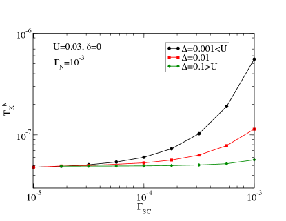
Figure 16: (Color online) NRG results for the Kondo temperature $T_{K}^{N}$ of the needle resonance as a function of the exchange coupling to the superconducting lead, $\Gamma_{SC}$, for several values of the BCS gap $\Delta$, both in the small $\Delta$ and large $\Delta$ limits.

Appendix C $\Gamma_{N}$ dependence of $T_{K}^{N}$

The $\Gamma_{N}$ dependence of the Kondo temperature $T_{K}^{N}$ is shown in Fig. 17. The behaviour for small $\Gamma_{N}$ is exponential, but with a non-standard factor in the exponent:

$$T_{K}^{N}\propto\exp\left(-c\frac{\pi U}{8\Gamma_{N}}\right),$$ (49)

where $c$ is a constant of order 1 which depends on $\Delta/U$ and $\Gamma_{SC}/U$ ratios; for parameters in the plot, we find $c=0.35$. For the standard single-impurity Anderson model with normal lead only, $c=1$. The deviation from $c=1$ (towards smaller values) indicates a renormalization of the charge fluctuation scale $U$ by the coupling to the superconducting lead. $c$ decreases ($U$ renormalizes more significantly) with increasing $\Gamma_{SC}$ and decreasing $\Delta$.

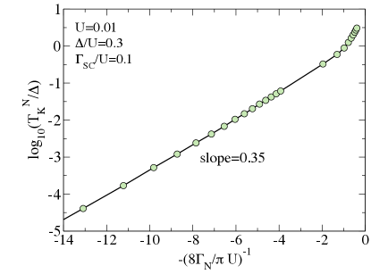
Figure 17: (Color online) NRG results for the Kondo temperature $T_{K}^{N}$ of the needle resonance as a function of the exchange coupling to the normal lead, $\Gamma_{N}$.

References

- (1) W.J. de Haas, J. de Boer and G. J. van dën Berg, The Electrical Resistance of Gold, Copper and Lead at Low Temperatures, Commun. Kamerlingh Onnes Lab., Leiden 233b; Physica, 1, 1115 (1934).
- (2) J. Kondo, Resistance Minimum in Dilute Magnetic Alloys, Prog. Theor. Phys. 32, 37 (1964).
- (3) A. C. Hewson, Renormalized Perturbation Expansions and Fermi Liquid Theory, Phys. Rev. Lett. 70, 4007 (1993).
- (4) D. Goldhaber-Gordon et al., Kondo Effect in a Single-Electron Transistor, Nature 391, 156 (1998); S. M. Cronenwett, T. H. Oosterkamp, and L. P. Kouwenhoven, A Tunable Kondo Effect in Quantum Dots, Science 281, 540 (1998); L. P. Kouwenhoven, and L. Glazman, The Revival of the Kondo Effect, Physics World 33 (2001).
- (5) Jesper Nygard, David Henry Cobden, and P. Erik Lindelof, Kondo Physics in Carbon Nanotubes, Nature 408, 342 (2000); C. H. L. Quay, J. Cumings, S. J. Gamble, R. de Picciotto, H. Kataura, and D. Goldhaber-Gordon, Magnetic Field Dependence of the Spin- and Spin-1 Kondo Effects in a Quantum Dot, Phys. Rev. B 76, 245311 (2007).
- (6) T. S. Jespersen, M. Aagesen, C. Sorensen, P. E. Lindelof, and J. Nygard, Kondo Physics in Tunable Semiconductor Nanowire Quantum Dots, Phys. Rev. B 74, 233304 (2006); S. Csonka, L. Hofstetter, F. Freitag, S. Oberholzer, C. Schoenenberger, T. S. Jespersen, M. Aagesen, and J. Nygard, Giant Fluctuations and Gate Control of the g-Factor in InAs Nanowire Quantum Dots, Nano Lett. 8, 3932 (2008); H. A. Nilsson, P. Caroff, C. Thelander, M. Larsson, J. B. Wagner, L.-E. Wernersson, L. Samuelson, and H. Q. Xu, Giant, Level-Dependent g Factors in InSb Nanowire Quantum Dots, Nano Lett. 9, 3151 (2009); A. V. Kretinin, R. Popovitz-Biro, D. Mahalu, and H. Shtrikman, Multimode Fabry-Perot Conductance Oscillations in Suspended Stacking-Faults-Free InAs Nanowires, Nano Lett. 10, 3439 (2010).
- (7) S. De Franceschi, L. P. Kouwenhoven, C. Schönenberg, and W. Wernsdorfer, Hybrid Superconductor-Quantum Dot Devices, Nature Nanotechnology 5, 703 (2010).
- (8) Yu Luh, Acta Phys. Sin. Bound State in Superconductors with Paramagnetic Impurities, 21, 75 (1965); H. Shiba, Classical Spins in Superconductors, Prog.Theor. Phys. 40, 435 (1968); A.I. Rusinov, On the Theory of Gapless Superconductivity in Alloys Containing Paramagnetic Impurites, Sov. Phys. JETP 29, 1101 (1969); H. Shiba and T. Soda, Superconducting Tunneling through the Barrier with Paramagnetic Impurities, Prog. Theor. Phys. 41, 25 (1969).
- (9) A.V. Balatsky, I. Vekhter, and J.-X. Zhu, Impurity-Induced States in Conventional and Unconventional Superconductors, Rev. Mod. Phys. 78, 373 (2006).
- (10) A. Sakurai, Comments on Superconductors with Magnetic Impurities, Prog. Theor. Phys. 44, 1472 (1970).
- (11) O. Sakai, Y. Shimizu, H. Shiba, and K. Satori, Numerical Renormalization Group Study of Magnetic Impurities in Superconductors. II. Dynamical Excitation Spectra and Spatial Variation of the Order Parameter, J. Phys. Soc. Jpn. 62, 3181 (1993).
- (12) T. Sand-Jespersen et al, Kondo-Enhanced Andreev Tunneling in InAs Nanowire Quantum Dots, Phys. Rev. Lett. 99,126603 (2007).
- (13) A. Eichler et al, Even-Odd Effect in Andreev Transport through a Carbon Nanotube Quantum Dot, Phys. Rev. Lett. 99,126602 (2007).
- (14) K. Grove-Rasmussen et al, Superconductivity-Enhanced Bias Spectroscopy in Carbon Nanotube Quantum Dots, Phys. Rev. B, 79, 134518 (2009).
- (15) J.-D. Pillet, C. H. L. Quay, P. Morfin, C. Bena, A. Levy-Yeyati, and P. Joyez, Andreev Bound States in Supercurrent-Carrying Carbon Nanotubes Revealed, Nat. Phys. 6, 965 (2010).
- (16) R. S. Deacon, Y. Tanaka, A. Oiwa, R. Sakano, K. Yoshida, K. Shibata, K. Hirakawa, and S. Tarucha, Tunneling Spectroscopy of Andreev Energy Levels in a Quantum Dot Coupled to a Superconductor, Phys. Rev. Lett. 104, 076805 (2010).
- (17) T. Dirks, T. L. Hughes, S. Lal, B. Uchoa, Y. Chen, C. Chialvo, P. M. Goldbart, and N. Mason, Transport through Andreev Bound States in a Graphene Quantum Dot, Nature Physics 7, 386, (2011).
- (18) B. M. Andersen, K. Flensberg, V. Koerting, and J. Paaske, Nonequilibrium Transport through a Spinful Quantum Dot with Superconducting Leads, Phys. Rev. Lett. 107, 256802 (2011).
- (19) E. J. H. Lee, X. Jiang, R. Aguado, G. Katsaros, C. M. Lieber, and S. De Franceschi, Zero-Bias Anomaly in a Nanowire Quantum Dot Coupled to Superconductors, Phys. Rev. Lett. 109, 186802 (2012).
- (20) B.-K. Kim, Y.-H. Ahn, J.-J. Kim, M.-S. Choi, M.-H. Bae, K. Kang, J. S. Lim, R. Lopez, and N. Kim, Transport Measurement of Andreev Bound States in a Kondo-Correlated Quantum Dot, Phys. Rev. Lett. 110, 076803 (2013).
- (21) W. Chang, V. E. Manucharyan, T. S. Jespersen, J. Nygard, and C. M. Marcus, Tunneling Spectroscopy of Quasiparticle Bound States in a Spinful Josephson Junction, Phys. Rev. Lett. 110, 217005 (2013).
- (22) J.-D. Pillet, P. Joyez, R. Žitko, and M. F. Goffman, Tunneling Spectroscopy of a Single Quantum Dot Coupled to a Superconductor: From Kondo Ridge to Andreev Bound States, Phys. Rev. B 88, 045101 (2013).
- (23) A. Kumar, M. Gaim, D. Steininger, A. Levy Yeyati, A. Martín-Rodero, A. K. Hüttel, and C. Strunk, Temperature Dependence of Andreev Spectra in a Superconducting Carbon Nanotube Quantum Dot, Phys. Rev. B 89, 075428 (2014).
- (24) J. Schindele, A. Baumgartner, R. Maurand, M. Weiss, and C. Schönenberger, Nonlocal Spectroscopy of Andreev Bound States, Phys. Rev. B 89, 045422 (2014).
- (25) E. J. H. Lee, X. Jiang, M. Houzet, R. Aguado, C. M. Lieber, and S. De Franceschi, Spin-Resolved Andreev Levels and Parity Crossings in Hybrid Superconductor-Semiconductor Nanostructures, Nature Nanotechnology 9, 79 (2014).
- (26) K. J. Franke, G. Schulze, and J. I. Pascual, Competition of Superconducting Phenomena nad Kondo Screening at the Nanoscale, Science 332, 940 (2011).
- (27) For reviews, see J. Alicea, New Directions in the Pursuit of Majoranan Fermions in Solid State Systems, Rep. Prog. Phys. 75, 076501, (2012); C. Beenakker, Search for Majorana Fermions in Superconductors, Annu. Rev. Cond. Mat. Phys. 4, 113, (2013); T. Stanescu and S. Tewari, Majorana Fermions in Semiconductor Nanowires: Fundamentals, Modeling, and Experiment, J. Phys. Condens. Matter 25, 233201, (2013).
- (28) R. M. Lutchyn, J. D. Sau and S. Das Sarma, Majorana Fermions and a Topological Phase Transition in Semiconductor-Superconductor Heterostructures, Phys. Rev. Lett. 105, 077001 (2010).
- (29) Y. Oreg, G. Refael, and F. von Oppen, Helical Liquids and Majorana Bound States in Quantum Wires, Phys. Rev. Lett. 105, 177002 (2010).
- (30) V. Mourik, K. Zuo, S. M. Frolov, S. R. Plissard, E. P. A. M. Bakkers, and L. P. Kouwenhoven, Signatures of Majorana Fermions in Hybrid Superconductor-Semiconductor Nanowire Devices, Science 336, 1003 (2012).
- (31) A. Das, Y. Ronen, Y. Most, Y. Oreg, M. Heiblum, and H. Shtrikman, Zero-Bias Peaks and Splitting in an Al-InAs Nanowire Topological Superconductor as a Signature of Majorana Fermions, Nat. Phys. 8, 887 (2012).
- (32) M. T. Deng, C. L. Yu, G. Y. Huang,. M. Larsson, P. Caroff, and H. Q. Xu, Anomalous Zero-Bias Conductance Peak in a Nb-InSb Nanowire-Nb Hybrid Device, Nano Lett. 12, 6414 (2012).
- (33) A. D. K. Finck, D. J. Van Harlingen, P. K. Mohseni, K. Jung, and X. Li, Anomalous Modulation of a Zero-Bias Peak in a Hybrid Nanowire-Superconductor Device, Phys. Rev. Lett. 110, 126406 (2013).
- (34) H. O. H. Churchill, V. Fatemi, K. Grove-Rasmussen, M. T. Deng, P. Caroff, H. Q. Xu, and C. M. Marcus, Superconductor-Nanowire Devices from Tunneling to the Multichannel Regime: Zero-Bias Oscillations and Magnetoconductance Crossover, Phys. Rev. B, 87, 241401 (2013).
- (35) In particular, single Zeeman crossings evolve into multiple crossing showing oscillatory behavior versus magnetic field, see also J. S. Lim, L. Serra, R. López, and R. Aguado, Magnetic-Field Instability of Majorana Modes in Multiband Semiconductor Wires, Phys. Rev. B 86, 121103 (2012); E. Prada, P. San-Jose and R. Aguado, Transport Spectroscopy of Nanowire Junctions with Majorana Fermions, Phys. Rev. B 86, 180503 (2012); D. Rainis, L. Trifunovic, J. Klinovaja, and D. Loss, Towards a Realistic Transport Modeling in a Superconducting Nanowire with Majorana Fermions, Phys. Rev. B 87, 024515 (2013); S. Das Sarma, Jay D. Sau and T. D. Stanescu, Splitting of the Zero-Bias Conductance Peak as Smoking Gun Evidence for the Existence of the Majorana Mode in a Superconductor-Semiconductor Nanowire, Phys. Rev. B 86, 220506 (2013).
- (36) T. D. Stanescu, R. M. Lutchyn, and S. Das Sarma, Dimensional Crossover in Spin-Orbit-Coupled Semiconductor Nanowires with Induced Superconducting Pairing, Phys. Rev. B 87, 094518 (2013).
- (37) T.-P. Choy, J. M. Edge, A. R. Akhmerov, and C. W. J. Beenakker, Majorana Fermions Emerging from Magnetic Nanoparticles on a Superconductor without Spin-Orbit Coupling, Phys. Rev. B 84, 195442 (2011); S. Nadj-Perge, I. K. Drozdov, B. A. Bernevig, and A. Yazdani, Proposal for Realizing Majorana Fermions in Chains of Magnetic Atoms on a Superconductor, Phys. Rev. B 88, 020407 (2013); B. Braunecker and P. Simon, Interplay between Classical Magnetic Moments and Superconductivity in Quantum One-Dimensional Conductors: Toward a Self-Sustained Topological Majorana Phase, Phys. Rev. Lett. 111, 147202 (2013); F. Pientka, L. I. Glazman and F. von Oppen, Topological Superconducting Phase in Helical Shiba Chains, Phys. Rev. B 88, 155420 (2013); J. Klinovaja, P. Stano, A. Yazdani, and D. Loss, Topological Superconductivity and Majorana Fermions in RKKY Systems, Phys. Rev. Lett. 111, 186805 (2013); S. Nakosai, Y. Tanaka, and N. Nagaosa, Two-Dimensional -Wave Superconducting States with Magnetic Moments on a Conventional -Wave Superconductor, Phys. Rev. B 88, 180503 (2013); M. M. Vazifeh and M. Franz, Self-Organized Topological State with Majorana Fermions, Phys. Rev. Lett. 111, 206802 (2013); P. M. R. Brydon, H. Hui and J. D. Sau, Topological Shiba Chain from Spin-Orbit Coupling, arXiv:1407.6345 (2014).
- (38) Stevan Nadj-Perge,Ilya K. Drozdov, Jian Li, Hua Chen, Sangjun Jeon, Jungpil Seo, Allan H. MacDonald, B. Andrei Bernevig, Ali Yazdani, Observation of Majorana Fermions in Ferromagnetic Atomic Chains on a Superconductor, Science 346, 602 (2014).
- (39) Yang Peng, Falko Pientka, Leonid I. Glazman, Felix von Oppen, Strong Localization of Majorana End States in Chains of Magnetic Adatoms, arXiv:1412.0151 (2014).
- (40) A. Martin-Rodero and A. Levy-Yeyati, Josephson and Andreev Transport through Quantum Dots, Adv. Phys. 60, 899 (2011).
- (41) V. Koerting, B. M. Andersen, K. Flensberg, and J. Paaske, Nonequilibrium Transport via Spin-Induced Subgap States in Superconductor/Quantum Dot/Normal Metal Cotunnel Junctions, Phys. Rev. B, 82, 245108 (2011).
- (42) Y. Yamada, Y. Tanaka and N. Kawakami, Interplay of Kondo and Superconducting Correlations in the Nonequilibrium Andreev Transport through a Quantum Dot, Phys. Rev. B, 84, 075484 (2011).
- (43) J. Barański and T. Domański, In-Gap States of a Quantum Dot Coupled between a Normal and a Superconducting Lead, J. Phys.: Condens. Matter 25, 435305 (2013).
- (44) M. Zapalska and T. Domanski, Kondo Impurity between Superconducting and Metallic Reservoir: the Flow Equation Approach, arXiv:1402.1291 (2014).
- (45) K. G. Wilson, The Renormalization Group: Critical Phenomena and the Kondo Problem, Rev. Mod. Phys. 47, 773 (1975).
- (46) H. R. Krishna-murthy, J. W. Wilkins, and K. G. Wilson, Renormalization-Group Approach to the Anderson Model of Dilute Magnetic Alloys. I. Static Properties for the Symmetric Case, Phys. Rev. B 21, 1003 (1980); Renormalization-Group Approach to the Anderson Model of Dilute Magnetic Alloys. II. Static Properties for the Asymmetric Case, ibid., 21, 1044 (1980).
- (47) W. Hofstetter, Generalized Numerical Renormalization Group for Dynamical Quantities, Phys. Rev. Lett. 85, 1508 (2000).
- (48) R. Bulla, T. A. Costi, and T. Pruschke, Numerical Renormalization Group Method for Quantum Impurity Systems, Rev. Mod. Phys. 80, 395 (2008).
- (49) Y. Tanaka, N. Kawakami and A. Oguri, Numerical Renormalization Group Approach to a Quantum Dot Coupled to Normal and Superconducting Leads, J. Phys. Soc. Japan, 76, 074701 (2007).
- (50) A. Oguri, Y. Tanaka and J. Bauer, Interplay between Kondo and Andreev-Josephson Effects in a Quantum Dot Coupled to One Normal and Two Superconducting Leads, Phys. Rev. B, 87, 075432 (2013).
- (51) Y. Meir and N. S. Wingreen, Spin-Orbit Scattering and the Kondo Effect, Phys. Rev. B 50, 4947 (1994).
- (52) R. Žitko, Quantum Impurity on the Surface of a Topological Insulator, Phys. Rev. B 81, 241414(R) (2010).
- (53) J. Malecki, The Two Dimensional Kondo Model with Rashba Spin-Orbit Coupling, J. Stat. Phys. 129, 741 (2007).
- (54) R. Žitko and J. Bonča, Kondo Effect in the Presence of Rashba Spin-Orbit Interaction, Phys. Rev. B 84, 193411 (2011).
- (55) A. Weichselbaum and Jan von Delft, Sum-Rule Conserving Spectral Functions from the Numerical Renormalization Group, Phys. Rev. Lett. 99, 076402 (2007).
- (56) J. R. Schrieffer and P. A. Wolff, Relation between the Anderson and Kondo Hamiltonians, Phys. Rev. 149, 491 (1996).
- (57) N. N. Bogoliubov, On a New Method in the Theory of Superconductivity, Nuovo Cimento 7, 794 (1958).
- (58) N. N. Bogoliubov, A New Method in the Theory of Superconductivity. I, Sov. Phys. JETP 7, 41 (1958).
- (59) J. G. Valatin, Comments on the Theory of Superconductivity, Nuovo Cimento 7, 843 (1958).
- (60) M. M. Salomaa, Schrieffer-Wolff Transformation for the Anderson Hamiltonian in a Superconductor, Phys. Rev. B 37, 9312 (1988).