Quantum critical point in the superconducting transition on the surface of topological insulator

Abstract

Pairing in the Weyl semi - metal appearing on the surface of topological insulator is considered. It is shown that due to an ”ultra-relativistic” dispersion relation there is a quantum critical point governing the zero temperature transition to a superconducting state. Starting from the microscopic Hamiltonian with local attraction, we calculated using the Gor’kov equations, the phase diagram of the superconducting transition at arbitrary chemical potential, its magnetic properties and critical exponents close to the quantum critical point. The Ginzburg - Landau effective theory is derived for small chemical potential allowing to consider effects of spatial dependence of order parameters in magnetic field. The GL equations are very different from the conventional ones reflecting the chiral universality class of the quantum phase transition. The order parameter distribution of a single vortex is found to be different as well. The magnetization near the upper critical field is found to be quadratic, not linear as usual. We discuss the application of these results to recent experiments in which surface superconductivity was found that some 3D topological insulators and estimate feasibility of the phonon pairing.

I Introduction

Topological insulator (TI) is a novel state of matter in materials with strong spin - orbit interactions that create topologically protected surface states Zhang . The electrons (holes) in these states have a linear dispersion relation and can be described approximately by a (pseudo) relativistic two dimensional (2D) Weyl Hamiltonian. The system with the chemical potential above or below the Weyl point realizes an ”ultra-relativistic” 2D electron or hole conducting liquid. It is known for a long time that similar 2D and quasi-2D metallic systems like the surface metal on twin planes Shapiro , layered materials (strongly anisotropic high $T_{c}$ cupratesWen or organic superconductorsorganic ) may develop 2D (surface) superconductivity. This phenomenon became known as ”localized superconductivity”Buzdin . Since best studied TIs possess a quite standard phonon spectrum phononexp , it was predicted recently DasSarma that they become superconducting TI (STI) (this should be distinguished from ”topological superconductors”, TSC, in which superconductivity appears in the bulk Zhang ). The predicted critical temperature of order of $1K$ is rather low (despite a fortunate suppression of the Coulomb repulsion due to a large dielectric constant $\varepsilon\sim 50$), the nature of the ”normal” state (so-called 2D Weyl semi-metal) might make the superconducting properties of the system unusual. The ultra-relativistic nature manifests itself mostly when the Weyl cone is very close to the Fermi surface. Especially interesting is the case (that actually was originally predicted for the [111] surface of $Bi_{2}Te_{3}$ and $Bi_{2}Se_{3}$Zhang1 ) when the chemical potential coincides with the Weyl point. Although subsequent ARPES experimentsZhang show the location of the cone of surface states order tenths of $eV$ off the Fermi surface; there are experimental means to shift the chemical potential, for example by the bias voltage bias .

Unlike the more customary poor 2D metals with several small pockets of electrons/holes on the Fermi surface (in semiconductor systems or even some high $T_{c}$ materialsWen ), the electron gas STI has two peculiarities especially important when pairing is contemplated. The first is the bipolar nature of the Weyl spectrum: there is no energy gap between the upper and lower cones. The second is that  the spin degree of freedom is a major player in the quasiparticle dynamics. This degree of freedom determines the pairing channel. The pairing channel problem was studied theoretically on the level of the Bogoliubov-deGennes equation Herbut . Both $s$-wave and $p$-wave are possible and compete due to the breaking of the bulk inversion symmetry by the surface. The spectrum of Andreev states of the Abrikosov vortex was obtainedNori in a related problem of TI in contact with an $s$-wave superconductor DasSarma1 . Various pairing interactions were considered to calculate the DOS measured in $Cu_{x}Bi_{2}Se_{3}$ to discriminate between STI and TSC using self-consistent analysis Sato . As mentioned above the most intriguing case is that of the small chemical potential that has not been addressed microscopically. It turns out that it is governed by a quantum critical point (QCP)Sachdev .

The concept of QCP at zero temperature and varying doping constitutes a very useful language for describing the microscopic origin of superconductivity in high $T_{c}$ cuprates and other ”unconventional” superconductorsWen . Superconducting transitions generally belong to the $U\left(1\right)$ class of second order phase transitionsLandau , however it was pointed out a long time agoRosenstein that, if the normal state dispersion relation is ”ultra-relativistic”, the transition at zero temperature as function of parameters like the pairing interaction strength is qualitatively distinct and belongs to chiral universality classes classified in ref. Gat . Attempts to experimentally identify second order transitions governed by QCP included quantum magnets Sachdev , superconductor - insulator transitionsSCinsulator and more recently chiral condensate in grapheneKatsnelson ; CastroNeto .

In this paper we study the thermodynamic and magnetic properties of the surface superconductivity in TI with local attraction pairing Hamiltonian characterized by the coupling strength $g$ and cutoff parameter $T_{D}$ within the self-consistent approximation. The phase diagram for $s$-wave pairing is obtained for arbitrary temperature $T$ and chemical potential $\mu<T_{D}$. The latter condition is the main difference from the conventional BCS model in which $\mu>>T_{D}$. We found a quantum critical point at $T=\mu=0$ when the coupling strength $g$ reaches a critical value $g_{c}$ dependent on the cutoff parameter. We concentrate on properties of the superconducting state in a part of the phase diagram that is dominated by the QCP. Various critical exponents are obtained. In particular, the coupling strength dependence of the coherence length is $\xi\propto\left(g-g_{c}\right)^{-\nu}$ with $\nu=1$ , the order parameter scales as $\Delta\propto\left(g-g_{c}\right)^{\beta}$, $\beta=1$. It is found that near the QCP the Ginzburg - Landau effective model is rather unconventional. The structure of the single vortex core is different from the usual Abrikosov vortex, while the magnetization curve near the upper critical magnetic field $H_{c2}$ is quadratic: $M=\left(H-H_{c2}\right)^{2}$, not linear.

The rest of the paper is organized as follows. The model and the method of its solution (in the Gorkov equations form) are presented in Section II. The phase diagram in the homogeneous case (no magnetic field) is established and the unusual nature of the phase transition discussed. The novel case of zero chemical potential (tuning to the Weyl point) is studied in detail. The Ginzburg-Landau energy is derived in Section III and exploited to determine magnetic properties of STI. The $H_{c2}$ line and magnetization curves for a dense vortex lattice as well as the single vortex texture are obtained. Section IV contains discussion on experimental feasibility of the phonon mediated surface superconductivity in TI, comparison with more familiar BEC and BCS scenarios and conclusion.

II The s-wave pairing model. The phase diagram.

II.1 TI in magnetic field with a local pairing interaction. Gor’kov equations.

Electrons on the surface of a TI perpendicular to $z$ axis, see Fig.1, are described by a Pauli spinor $\psi_{\alpha}\left(\mathbf{r}\right)$, where the upper plane, $\mathbf{r}=\left\{x,y\right\}$, is considered, with spin projections taking the values $\alpha=\uparrow,\downarrow$ with respect to $z$ axis. The Hamiltonian for electrons in TI subjected to a perpendicular external homogeneous magnetic field, and interacting via four-Fermi local coupling of strength $g$ is

$$H = \int d^{2}r\left\{\psi_{\alpha}^{+}\left(\mathbf{r}\right)\widehat{H}_{\alpha\beta}\psi_{\beta}\left(\mathbf{r}\right)\right.$$

$$\left.\mathbf{-}\frac{g}{2}\psi_{\alpha}^{+}\left(\mathbf{r}\right)\psi_{\beta}^{+}\left(\mathbf{r}\right)\psi_{\beta}\left(\mathbf{r}\right)\psi_{\alpha}\left(\mathbf{r}\right)\right\}+H_{mag}\text{.}$$

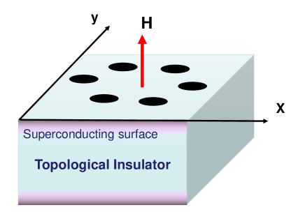
Figure 1: Topological insulator plate in magnetic field. Surfaces are populated by Weyl quasiparticles and holes that both can be paired by interactions. Magnetic field creates vortices with normal cores (dark areas on the surfaces) of the radius of order of coherence length $\xi$.

Here the surface Weyl Hamiltonian matrix Zhang ; Herbut is defined as

$$\widehat{H}_{\alpha\beta} = v_{F}\varepsilon_{ij}\widehat{P}_{i}\sigma_{\alpha\beta}^{j}-\mu\delta_{\alpha\beta}\text{;}$$ (2)

$$\widehat{\mathbf{P}} \equiv -i\hbar\mathbf{\nabla-}\frac{e^{\ast}}{c}\mathbf{A}\left(\mathbf{r}\right)\text{,}$$

where $i,j=x,y$; $v_{F}$ is the Fermi velocity of the TI and $\mu$ is the surface chemical potential. $\sigma^{j}$ are the Pauli matrices and $\varepsilon_{ij}$ is the antisymmetric tensor. Only one valley is explicitly considered (generalization to several ”flavors” is trivial). Vector potential $\mathbf{A}$ describes the 3D magnetic induction $\mathbf{B}=\mathbf{\nabla\times A}$ with magnetic energy given by

$$H_{mag}=\frac{1}{8\pi}\int d^{2}rdz\left(\mathbf{B}\left(\mathbf{r,}z\right)-\mathbf{H}_{ext}\right)^{2}\text{.}$$ (3)

The effective local interaction might be generated by a phonon exchange or perhaps other mechanisms and will be assumed to be weak coupling. Therefore the BCS type approximation can be employed. Using the standard formalism, the Matsubara Green’s functions ($\tau$ is the Matsubara time),

$$G_{\alpha\beta}\left(\mathbf{r},\tau;\mathbf{r}^{\prime},\tau^{\prime}\right) = -\left\langle T_{\tau}\psi_{\alpha}\left(\mathbf{r},\tau\right)\psi_{\beta}^{\dagger}\left(\mathbf{r}^{\prime},\tau^{\prime}\right)\right\rangle\text{;}$$ (4)

$$F_{\alpha\beta}^{\dagger}\left(\mathbf{r},\tau;\mathbf{r}^{\prime},\tau^{\prime}\right) = \left\langle T_{\tau}\psi_{\alpha}^{\dagger}\left(\mathbf{r},\tau\right)\psi_{\beta}^{\dagger}\left(\mathbf{r}^{\prime},\tau^{\prime}\right)\right\rangle\text{,}$$

obey the Gor’kov equationsAGD :

$$-\frac{\partial G_{\gamma\kappa}\left(\mathbf{r},\tau;\mathbf{r}^{\prime},\tau^{\prime}\right)}{\partial\tau}-\int_{\mathbf{r}^{\prime\prime}}\left\langle\mathbf{r}\left|\widehat{H}_{\gamma\beta}\right|\mathbf{r}^{\prime\prime}\right\rangle G_{\beta\kappa}\left(\mathbf{r}^{\prime\prime},\tau;\mathbf{r}^{\prime},\tau^{\prime}\right)$$ (5)

$$-gF_{\beta\gamma}\left(\mathbf{r},\tau;\mathbf{r},\tau\right)F_{\beta\kappa}^{\dagger}\left(\mathbf{r},\tau,\mathbf{r}^{\prime},\tau^{\prime}\right)=\delta^{\gamma\kappa}\delta\left(\mathbf{r-r}^{\prime}\right)\delta\left(\tau-\tau^{\prime}\right);$$

$$\frac{\partial F_{\gamma\kappa}^{\dagger}\left(\mathbf{r},\tau;\mathbf{r}^{\prime},\tau^{\prime}\right)}{\partial\tau}-\int_{\mathbf{r}^{\prime\prime}}\left\langle\mathbf{r}\left|\widehat{H}_{\gamma\beta}^{t}\right|\mathbf{r}^{\prime\prime}\right\rangle F_{\beta\kappa}^{\dagger}\left(\mathbf{r}^{\prime\prime},\tau;\mathbf{r}^{\prime},\tau^{\prime}\right)$$

$$-gF_{\gamma\beta}^{\dagger}\left(\mathbf{r},\tau;\mathbf{r},\tau\right)G_{\beta\kappa}\left(\mathbf{r},\tau,\mathbf{r}^{\prime},\tau^{\prime}\right)=0\text{.}$$

In the presence of magnetic field these equations are complicated by emergence of inhomogeneity pertinent to type II superconductors. This will be addressed in Section III. Here we solve the homogeneous case when no magnetic field is present.

II.2 Uniform condensate.

In the homogeneous case the Gor’kov equations for Fourier components of the Greens functions simplify considerably,

$$D_{\gamma\beta}^{-1}G_{\beta\kappa}\left(\omega,p\right)-\widehat{\Delta}_{\gamma\beta}F_{\beta\kappa}^{\dagger}\left(\omega,p\right) = \delta^{\gamma\kappa}\text{;}$$ (6)

$$D_{\beta\gamma}^{-1}F_{\beta\kappa}^{\dagger}\left(\omega,p\right)+\widehat{\Delta}_{\gamma\beta}^{\ast}G_{\beta\kappa}\left(\omega,p\right) = 0\text{,}$$

where $\omega=\pi T\left(2n+1\right)$ is the Matsubara frequency and$\ D_{\gamma\beta}^{-1}=\left(i\omega-\mu\right)\delta_{\gamma\beta}-v_{F}\varepsilon_{ij}p_{i}\sigma_{\alpha\beta}^{j}$. The matrix gap function can be chosen as ($\Delta$ real)

$$\widehat{\Delta}_{\beta\gamma}=gF_{\gamma\beta}\left(0\right)=\left(\begin{array}[]{cc}0&\Delta\\ -\Delta&0\end{array}\right)\text{.}$$ (7)

These equations are conveniently presented in matrix form (superscript $t$ denotes transposed and $I$ - the identity matrix):

$$D^{-1}G-\widehat{\Delta}F^{\dagger} = I\text{;}$$ (8)

$$D^{t-1}F^{\dagger}+\widehat{\Delta}^{\ast}G = 0\text{.}$$

Solving these equations one obtains

$$G^{-1} = D^{-1}+\widehat{\Delta}D^{t}\widehat{\Delta}^{\ast}\text{;}$$ (9)

$$F^{\dagger} = -D^{t}\widehat{\Delta}^{\ast}G\text{,}$$

with the gap function found from the consistency condition

$$\widehat{\Delta}^{\ast}=-g\sum\limits_{\omega q}D^{t}\widehat{\Delta}^{\ast}G\text{.}$$ (10)

The off-diagonal component of this equation is:

$$\Delta =g\Delta\sum\limits_{\omega q}\left(\Delta^{2}+v_{F}^{2}p^{2}+\mu^{2}+\hbar^{2}\omega^{2}\right)$$ (11)

$$\times\frac{1}{\left(\Delta^{2}+\hbar^{2}\omega^{2}+\left(v_{F}p-\mu\right)^{2}\right)\left(\Delta^{2}+\hbar^{2}\omega^{2}+\left(v_{F}p+\mu\right)^{2}\right)}\text{.}$$

The spectrum of elementary excitations obtained from the poles of the Greens function coincides with that found within the Bogoliubov - de Gennes approach Herbut

$$E_{p}=\pm\sqrt{\Delta^{2}+\left(v_{F}p-\mu\right)^{2}}\text{.}$$ (12)

The solutions of the gap equation are presented in the next subsection for a general chemical potential and zero temperature, while more general situations (arbitrary temperature and magnetic field) in the most interesting case of $\mu=0$ are addressed in the next section.

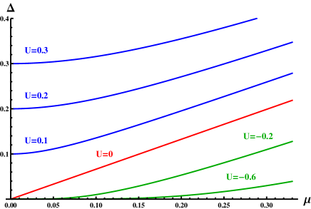
Figure 2: Order parameter at zero temperature as function of chemical potential of the TI surface Weyl semi-metal at various values of coupling parametrized by the renormalized energy $U$, Eq.(14). For positive $U$ (blue lines) the superconductivity is strong and does not vanish even for zero chemical potential. There exists the critical coupling, $U=0$ (red line), at which the second order transition occurs at quantum critical point $\mu=0$. For negative $U$ the superconductivity still exists at $\mu>0$, but is exponentially weak.

II.3 Zero temperature phase diagram and QCP.

At zero temperature the integrations over frequency and momentum limited by the UV cutoff $\Lambda$ result in (see Appendix A for details)

$$U\Delta=\Delta\left(\sqrt{\Delta^{2}+\mu^{2}}-\frac{\mu}{2}\log\frac{\sqrt{\Delta^{2}+\mu^{2}}+\mu}{\sqrt{\Delta^{2}+\mu^{2}}-\mu}\right)\text{,}$$ (13)

where the dependence on the cutoff is incorporated in the renormalized coupling with dimension of energy defined as

$$U=v_{F}\Lambda-\frac{4\pi\hbar^{2}v_{F}^{2}}{g}\text{.}$$ (14)

This can be interpreted as an effective binding energy of the Cooper pair in the Weyl semi - metal. For concreteness we consider only $\mu>0$, although the particle - hole symmetry makes the opposite case of the hole doping, $\mu<0$, identical. Of course the superconducting solution exists only for $g>0$. In Fig. 2 the dependence of the gap $\Delta$ as function of the chemical potential $\mu$ is presented for different values of $U$.

For an attractive coupling $g$ stronger than the critical one,

$$g_{c}=\frac{4\pi\hbar^{2}v_{F}}{\Lambda}\text{,}$$ (15)

(when $U>0$), blue lines in Fig. 2, there are two qualitatively different cases.

(i). When $\mu<<U$ the dependence of $\Delta$ on the chemical potential is parabolic, see Appendix B:

$$\frac{\Delta}{U}\approx 1+\left(\frac{\mu}{U}\right)^{2}\text{.}$$ (16)

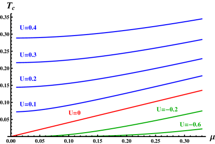
Figure 3: Transition temperature as function of chemical potential at supercritical ($U>0$, in blue), critical ($U=0$, in red) and subcritical values of coupling.

In particular, when $\mu=0,$ the gap equals $U$. As can be seen from Fig. 2, the chemical potential makes a very limited impact in the large portion of the phase diagram.

(ii) For the attraction just stronger than critical, $g>g_{c}$, namely for small positive $U$, the dependence becomes linear, see red line in Fig. 2, $\Delta=0.663\,\mu$. So that the already weak condensate becomes sensitive to $\mu$.

The case (i) is more interesting than (ii) since it exhibits stronger superconductivity (larger $T_{c}$, see below). Finally for $g<g_{c}\,$, namely negative $U$ (green lines in Fig. 2), the superconductivity is very weak with exponential dependence similar to the BCS one,

$$\Delta\approx\mu\text{ exp}\left[-\left(\left|U\right|/\mu-1\right)\right]\text{.}$$ (17)

More detailed comparisons will be performed in Section IV. As was mentioned above, in the more interesting cases of large $\Delta$ the dependence on the chemical potential is very weak. A peculiarity of superconductivity in TI is that electrons (and holes) in Cooper pairs are created themselves by the pairing interaction rather than being present in the sample as free electrons. Therefore it is shown that it is possible to neglect the effect of weak doping and consider directly the $\mu=0$ particle-hole symmetric case. This point in parameter space is the QCP Sachdev and will be studied in detail in what follows. Of course, at finite temperature at any attraction, $g>0$, there exists a (classical) superconducting critical point at certain temperature $T_{c}$ that is calculated next.

II.4 Dependence of the critical temperature $T_{c}$ on strength of pairing interaction.

Summation over Matsubara frequency and integrations over momenta in the gap equation, Eq.(13), at finite temperature and arbitrary chemical potential are performed in Appendix B. The critical temperature as a function of $\mu$ and (positive) $U$ is obtained numerically and presented in Fig. 3. Again at relatively large $U$ the dependence of $T_{c}$ on the chemical potential is very weak and parabolic. When $0<g<g_{c}$ the critical temperature is exponentially small albeit nonzero.

II.5 Zero chemical potential $\mu=0$.

At zero chemical potential the Hamiltonian Eq.(II.1) possesses a particle - hole symmetry. Microscopically, Cooper pairs of both electrons and holes are formed. The system is unique in this sense since the electron - hole symmetry is not spontaneously broken in both normal and superconducting phases. Supercurrent in such a system does not carry momentum or mass. Performing the sum and integral over momenta in the gap equation, Eq.(13), analytically (see Appendix A), it becomes (using the definition of $U$ given in Eq.(14)) for $U>0$:

$$U=2T\log\left[2\cosh\frac{\Delta}{2T}\right]\text{.}$$ (18)

At zero temperature $\Delta=U$, while $\Delta\rightarrow 0$ as a power of the parameter $U\propto g-g_{c}$ describing the deviation from quantum criticality

$$T_{c}=\frac{1}{2\log 2}U^{z\nu};\text{ \ }z\nu=1\text{.}$$ (19)

Here $z$ is the dynamical critical exponentSachdev . Therefore, as expected, the renormalized coupling describing the deviation from the QCP is proportional to the temperature at which the created condensate disappears.

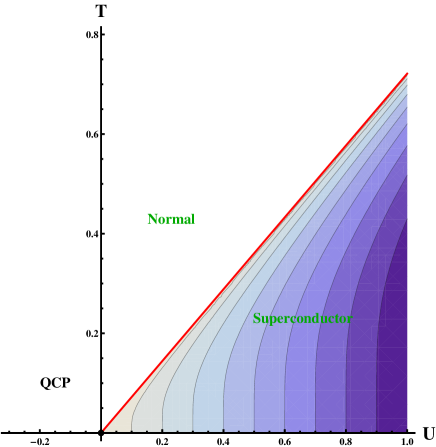
Figure 4: Phase diagram of  STI. Order parameter as function of chemical potential and temperature near the quantum critical point at $T=0$, $\mu=0$. The critical line is a strait line in mean field approximation.

The temperature dependence of the gap reads, see Fig. 4

$$\Delta\left(T\right)=2T\cosh^{-1}\left(\frac{1}{2}\exp\frac{U}{2T}\right)\text{.}$$ (20)

This it typical for chiral universality classes Sachdev ; Rosenstein .

It is interesting to compare this dependence with the conventional BCS for transition at finite temperature, namely away from QCP. At zero temperature $\Delta\left(0\right)/T_{c}=2\log 2$ $=\allowbreak 1.\,\allowbreak 39$ (within BCS - $1.76$), while near $T_{c}$ one gets $\Delta/T_{c}=2^{3/2}\log^{1/2}2\sqrt{1-t}=$ $2.\,\allowbreak 35\sqrt{1-t}$ (BCS - $3.07\sqrt{1-t}$), where $t=T/T_{c}$. To describe the behavior of the STI in inhomogeneous situations like the external magnetic field, boundaries, impurities or junction with metals or other superconductors, it is necessary to derive the effective theory in terms of the order parameter $\Delta\left(\mathbf{r}\right)$, where $\mathbf{r}$ varies on the mesoscopic scale.

III Ginzburg - Landau effective theory and magnetic properties of the superconductor near QCP

III.1 Coherence length and the condensation energy

Using the well known Gor’kov methodAGD , the quadratic term of the Ginzburg-Landau energy $F_{2}=\sum_{\mathbf{p}}\Delta_{p}^{\ast}\Gamma\left(p\right)\Delta_{p}$ is obtained exactly from expanding the gap equation to linear terms in $\Delta$ for arbitrary external momentum. The result derived in Appendix B reads:

$$\Gamma\left(p\right)=-\frac{U}{4\pi\hbar^{2}v_{F}^{2}}+\frac{\left|p\right|}{16v_{F}\hbar^{2}}\text{.}$$ (21)

The dependence on $\mathbf{p}$ is non-analytic and within our approximation higher powers of $p$ do not appear. The second term is very different from the quadratic term in the GL functional for conventional phase transitions at finite temperature Landau or even quantum phase transitions in models without Weyl fermions Sachdev and has a number of qualitative consequences. Comparing the two terms in Eq.(21), one obtains the coherence length as a power of parameter $U\propto g-g_{c}$ describing the deviation from criticality:

$$\xi\left(U\right)=\frac{\pi}{4}v_{F}\hbar U^{-\nu}\text{; \ \ \ \ }\nu=1\text{.}$$ (22)

This is different from the dependence in non-chiral universality classes that isLandau $\xi\left(T\right)\infty\left(T_{c}-T\right)^{-\nu},$ $\nu=1/2$ in mean field. Of course in the regime of critical fluctuations this exponent is corrected in both non-chiral Landau and chiralGat universality classes.

Local terms in the GL energy density are also calculable exactly (within our approximation, see Appendix C).

$$f_{cond}=\frac{1}{4\pi\hbar^{2}v_{F}^{2}}\left\{-U\Delta^{\ast}\Delta+\frac{2}{3}\left(\Delta^{\ast}\Delta\right)^{3/2}\right\}\text{.}$$ (23)

It is quite nonstandard compared to customary quartic term $\left(\Delta^{\ast}\Delta\right)^{2}$ in conventional universality classes. The GL equations in the homogeneous case for the condensate gives $\Delta_{0}=U^{\beta}$ with critical exponent $\beta=1,$ different from the mean field value $\beta=1/2$ for the $U\left(1\right)$ universality classLandau . The condensation energy density is $f_{0}=-\frac{1}{12\pi\hbar^{2}v_{F}^{2}}U^{2-\alpha}$ with $\alpha=-1$. The free energy critical exponent at QCP therefore is also different from the classical $\alpha=0$.

Having calculated both the local terms and the momentum dependence of the quadratic term in the Ginzburg - Landau energy, one is ready to formulate the GL energy in an inhomogeneous situations including magnetic field.

III.2 GL equations in the presence of magnetic field

In view of the local gauge invariance principle, replacing the momentum by a covariant derivative, the gradient term of the GL energy becomes

$$F_{grad}=\int d^{2}\mathbf{r}\frac{1}{16v_{F}\hbar}\Delta^{\ast}\left(\mathbf{r}\right)\sqrt{\left(-i\partial_{i}-\frac{e^{\ast}}{c\hbar}A_{i}\left(\mathbf{r}\right)\right)^{2}}\Delta\left(\mathbf{r}\right)\text{.}$$ (24)

This should be supplemented by the condensation energy Eq.(23) and magnetic energy Eq.(3). The GL equations are obtained by minimization with respect to 2D order parameter and 3D vector potential. In the present case the equation for the order parameter is nonlocal and nonanalytic:

$$\left\{\xi\sqrt{\left(-i\partial_{i}-\frac{e^{\ast}}{\hbar c}A_{i}\right)^{2}}-1\right\}\Delta+\frac{\Delta}{U}\left(\Delta^{\ast}\Delta\right)^{1/2}=0\text{.}$$ (25)

The supercurrent in the Maxwell equation,

$$\frac{c}{4\pi}\mathbf{\nabla}\times\mathbf{B}=\mathbf{J}\left(\mathbf{r}\right)\delta\left(z\right),$$ (26)

is also nonlocal: $J_{i}\left(\mathbf{r}\right)=\frac{1}{c}\frac{\delta F}{\delta A_{i}\left(\mathbf{r}\right)}$.

III.3 Upper critical field and the magnetization curve

The upper critical field is found from the spectrum of the gradient term operator in Eq.(25). The lowest eigenvalue of the operator for homogeneous induction $\mathbf{B}=\left\{0,0,B\right\}$ is $\xi\sqrt{e^{\ast}B/c\hbar}$ (the eigenvalue of the square root of an operator is a square root of the eigenvalue) and therefore the bifurcation occurs at

$$H_{c2}=\frac{\Phi_{0}}{2\pi\xi^{2}}\text{,}$$ (27)

with the coherence length $\xi$ found in Section II, Eq.(22). The formula is the same as in a more customary situation despite the fact that the coherence length has a different origin and different critical exponent at QCP.

Near $H_{c2}$ the Abrikosov hexagonal lattice is formed. Its energy density is approximated well using the lowest Landau level (LLL) approximation: $\Delta\left(\mathbf{r}\right)=\Delta_{A}\varphi\left(\mathbf{r}\right)$, where the Abrikosov hexagonal lattice function $\varphi$ is normalized by $\left\langle\left|\varphi\left(\mathbf{r}\right)\right|^{2}\right\rangle=1$ ($\left\langle...\right\rangle$ denotes here the space average). The strength of the condensate is determined by minimizing the energy (magnetic energy can be neglected):

$$\left\langle f\right\rangle = \frac{\left|\Delta_{A}\right|^{2}}{16v_{F}\hbar}\left\langle\varphi^{\ast}\left(\sqrt{\left(-i\partial_{i}-\frac{e^{\ast}}{c\hbar}A_{i}\left(\mathbf{r}\right)\right)^{2}}-\frac{4U}{\pi v_{F}\hbar}\right)\varphi\right\rangle$$

$$+\frac{\left|\Delta_{A}\right|^{3}}{6\pi\hbar^{2}v_{F}^{2}}\left\langle\left|\varphi\right|^{3}\right\rangle$$

$$= -\frac{\left|\Delta_{A}\right|^{2}}{32v_{F}\hbar}\sqrt{\frac{e^{\ast}}{c\hbar}}H_{c2}^{1/2}\left(1-H/H_{c2}\right)+\frac{\beta_{3}\left|\Delta_{A}\right|^{3}}{6\pi\hbar^{2}v_{F}^{2}}\text{.}$$

The number $\beta_{3}=\left\langle\left|\varphi\right|^{3}\right\rangle=1.07$ is analogous to $\beta_{A}$ for usual fourth power GL energy. The optimal $\Delta_{A}$ at external field $H$ close to $H_{c2}$ is:

$$\left|\Delta_{A}\right|=\frac{U}{2\sqrt{2\pi}\beta_{3}}\left(1-H/H_{c2}\right)^{\sigma}\text{; \ \ \ }\sigma=1\text{.}$$ (29)

This exponent for the transition on the $H_{c2}$ line is different from the ordinary Abrikosov latticeAbrikosov for which $\sigma=1/2$.

The magnetization is calculated from the averaged energy density for the optimal $\Delta_{A}$ given in Eq.(29) is ($B\simeq H$):

$$f\left(B\right)=-\frac{\sqrt{2\pi}}{3\cdot 2^{10}\beta_{3}}\frac{UH_{c2}}{\Phi_{0}}\left(1-H/H_{c2}\right)^{3}\text{.}$$ (30)

The dependence is quadratic,

$$M=-\frac{\pi^{3/2}}{2^{7}\sqrt{2}\beta_{3}}\frac{U}{\Phi_{0}}\left(1-H/H_{c2}\right)^{\tau}\text{, }\tau=2\text{, }$$ (31)

that should be contrasted with the usual linear dependenceAbrikosov , $\tau=1$. For smaller fields the vortex lattice becomes less dense and eventually the LLL approximation Li breaks down. However, since the superconductivity is confined to an atomic-width layer, there is no $H_{c1},$ and at small fields vortices become independent. Consequently the parabolic increase is halted and perfect diamagnetism appears only at $H=0$. Under these conditions we turn to a single vortex solution next.

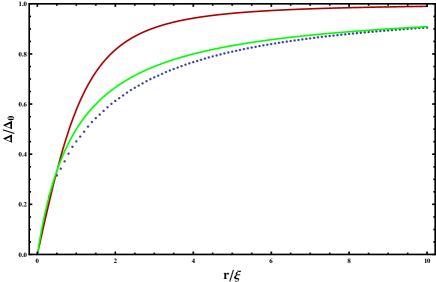
Figure 5: Vortex core structure near QCP. Order parameter in units of the bulk gap $\Delta_{0}$ as function of distance from the center in units of coherence length $\xi$. The blue line is the approximate formula, while the red line is the usual Abrikosov vortex profile.

III.4 Core structure of a single vortex

The single vortex solution for the order parameter can be found using the rotational symmetry in polar coordinates: $\Delta=Uf\left(r\right)e^{i\phi}$ with the homogeneous condensate value $\Delta=U$ found in Section II, so that at large distances the dimensionless order parameter $f\left(r\right)\rightarrow 1$. At the center of the vortex $f$ vanishes. The effects of the magnetic field, other than the phase rotation, are small in this extreme type II case of a surface superconductor Abrikosov . In this case the GL equation Eq.(25), using the coherence length $\xi$, Eq.(22) as unit of length, $\mathbf{r}\rightarrow\xi\mathbf{r\,}$, takes the form:

$$\left(\sqrt{\widehat{L}}-1\right)f\left(r\right)+f\left(r\right)^{2}=0\text{.}$$ (32)

The operator $\widehat{L}\equiv-\partial_{r}^{2}-\frac{1}{r}\partial_{r}+\frac{1}{r^{2}}$ has Bessel functions as its eigenvectors,

$$\left(-\partial_{r}^{2}-\frac{1}{r}\partial_{r}+\frac{1}{r^{2}}\right)J_{1}\left(\alpha r\right)=\alpha^{2}J_{1}\left(\alpha r\right)\text{.}$$ (33)

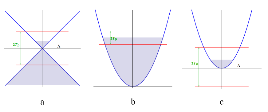
Figure 6: Schematic picture of the band reconstruction due to phonon pairing in three different 2D fermionic systems. a. Weyl semi-metal. b. BEC with parabolic dispersion law. c. Classic BCS.

Looking for the solution expanded in full set of these functions for all $\alpha$ satisfying our boundary conditions (Hankel transform) in the form

$$f\left(r\right)=1-\int_{\alpha=0}^{\infty}\alpha F\left(\alpha\right)J_{1}\left(\alpha r\right)\text{,}$$ (34)

the equation becomes

$$\int_{\alpha=0}^{\infty}F\left(\alpha\right)\alpha\left(\alpha+1\right)J_{1}\left(\alpha r\right)=\left(\int_{\beta=0}^{\infty}\beta F\left(\beta\right)J_{1}\left(\beta r\right)\right)^{2}\text{.}$$ (35)

To obtain an iterative form we multiply by $rJ_{1}\left(\gamma r\right),$ and integrating over $r$ using explicit formulas Auluck given in Appendix D results in

$$F\left(\gamma\right)=\frac{1}{\pi\left(\gamma+1\right)}\int_{\alpha,\beta=0}^{\infty}\frac{F\left(\alpha\right)F\left(\beta\right)(\alpha^{2}+\beta^{2}-\gamma^{2})}{\sqrt{\left(\gamma^{2}-\left(\alpha-\beta\right)^{2}\right)\left(\left(\alpha+\beta\right)^{2}-\gamma^{2}\right)}}\text{.}$$ (36)

The iteration converges very fast with the result presented in Fig. 5 (dots). The asymptotic at small $r$ is linear, $f\left(r\right)=r,$ while at large $r$ as expected it approaches the ”bulk” value $f\left(r\right)\rightarrow 1,$ and can be approximated by a formula $f\left(r\right)=\frac{r}{r+1}$ (green curve in Fig.5), simpler then the usual interpolation formula, $f\left(r\right)=\frac{r}{\sqrt{1+2r^{2}}}$ (orange curve in Fig.5). One observes that the relaxation of the order parameter away of the center of the vortex is much slower in STI..

IV Discussion and conclusions

IV.1 Comparison of renormalization of the coupling with BEC and BCS in 2D.

Let us contrast the coupling renormalization in a 2D Weyl semi-metal with momentum cutoff $\Lambda$ (for definiteness one can assume the phonon mechanism so that $\Lambda$ is the Debye cutoff $T_{D}$, under condition that the deviation from the Weyl point $\mu<<T_{D}$) with that in a 2D parabolic band, $E_{p}=\frac{p^{2}}{2m^{\ast}}$.The renormalized coupling, Eqs.(1514), can be written in the form

$$\frac{1}{g_{ren}}=\frac{1}{g}-\frac{\Lambda}{4\pi\hbar^{2}v_{F}}\text{,}$$ (37)

where $g_{ren}\equiv-4\pi\hbar^{2}v_{F}^{2}/U$. The linear renormalization (rather than the customary logarithmic cutoff dependence) of $\frac{1}{g}$ in Weyl semi-metal is pertinent to the so-called ”chiral universality classes” that sometimes appear in description of quantum critical points in 2DSachdev . It corresponds to finite coupling $g_{c}$ fixed points in Eqs.(14,15). This is the main difference from the more conventional cases that are briefly summarized next.

Within the parabolic case two cases are generally distinguishedStoof : the BCS, where the chemical potential $\mu$ is well above the bottom of the band, see Fig. 6, so that $T_{D}<<\mu$ (like in metallic superconductors), and the BEC when $\Lambda^{2}/2m^{\ast}>>\mu$, (like in cold atoms).

In BEC, that is closer to the STI considered here, the gap equation reads:

$$\frac{1}{g^{BEC}} = \frac{1}{2\pi}\int_{k=\hbar/L}^{\Lambda}\frac{k}{\sqrt{\left(k^{2}/2m^{\ast}-\mu\right)^{2}+\Delta^{2}}}$$ (38)

$$= \frac{m^{\ast}}{4\pi\hbar^{2}}\log\frac{\Lambda^{2}}{m^{\ast}\left(\sqrt{\mu_{ren}^{2}+\Delta^{2}}-\mu_{ren}\right)}\text{.}$$

Here $L$ is an infrared cutoff (needed in 2D) that is incorporated in $\mu_{ren}=\mu-\frac{\hbar^{2}}{2L^{2}m^{\ast}}$. The corresponding renormalized coupling depends on the reference (normalization) point $E_{ren}$ Shankar :

$$\frac{1}{g_{ren}^{BEC}}=\frac{1}{g^{BEC}}-\frac{m^{\ast}}{4\pi\hbar^{2}}\log\frac{\Lambda^{2}}{m^{\ast}E_{ren}}\text{.}$$ (39)

In terms of this coupling the theory becomes cutoff independent. For example, the gap equation reads:

$$\frac{1}{g_{ren}^{BEC}}=\frac{m^{\ast}}{4\pi\hbar^{2}}\log\frac{E_{ren}}{\sqrt{\mu_{ren}^{2}+\Delta^{2}}-\mu_{ren}}\text{.}$$ (40)

Table 1: Critical exponents of the chiral universality class of the TI QCP

critical exponent	order parameter	coherence length	energy	temperature
QCP $U_{1}\left(1\right)$ definition	$\Delta\propto U^{\beta}$	$\xi=U^{-\nu}$	$f\propto U^{2-\alpha}$	$T_{c}\propto U^{z\nu}$
meanfield value	$\beta=1$	$\nu=1$	$\alpha=-1$	$z\nu=1$
classical $U\left(1\right)$ definition	$\Delta\propto\left(T_{c}-T\right)^{\beta}$	$\xi\propto\left(T_{c}-T\right)^{-\nu}$	$f\propto\left(T_{c}-T\right)^{2-\alpha}$	–
mean field value	$\beta=\frac{1}{2}$	$\nu=\frac{1}{2}$	$\alpha=0$	–

Table 2: Critical exponents of the chiral universality class of the Abrikosov transition in external magnetic field at QCP.

critical exponent	magnetization	OP magnetic
QCP $U_{1}\left(1\right)$ definition	$M\propto\left(H_{c2}-H\right)^{\tau}$	$\Delta_{A}\propto\left(H_{c2}-H\right)^{\sigma}$
mean field value	$\tau=2$	$\sigma=1$
Abrikosov lattice definition	$M\propto\left(H_{c2}-H\right)^{\tau}$	$\Delta_{A}\propto\left(H_{c2}-H\right)^{\sigma}$
mean field value	$\tau=1$	$\sigma=\frac{1}{2}$

In BCS the gap equation, under the simplifying conditions $\mu>>T_{D}>\Delta$ (the dispersion relation near the Fermi level can be approximated by a ”flat” oneAGD ), is

$$\frac{1}{g^{BCS}} = \frac{1}{2\pi}\int_{k=\sqrt{2m^{\ast}\left(\mu-T_{D}\right)}}^{\sqrt{2m^{\ast}\left(\mu+T_{D}\right)}}\frac{k}{\sqrt{\left(k^{2}/2m^{\ast}-\mu\right)^{2}+\Delta^{2}}}$$ (41)

$$\simeq \frac{m^{\ast}}{2\pi\hbar^{2}}\log\frac{2T_{D}}{\Delta}\text{.}$$

The renormalized coupling is again dependent on an arbitrarily chosen normalization scale, $E_{ren}$,

$$\frac{1}{g_{ren}^{BCS}}=\frac{1}{g^{BCS}}-\frac{m^{\ast}}{2\pi\hbar^{2}}\log\frac{T_{D}}{E_{ren}}\text{.}$$

In both parabolic cases the coupling is logarithmically ”running” towards weak couplingShankar $g^{BCS}\rightarrow g_{c}=0$ (marginally irrelevant or asymptotically free) at large $\Lambda$. In the Weyl semimetal (where the dispersion is linear) with local interaction the criticality appears at small $U$ when $g$ approaches finite value $g_{c}$. Despite the fact that the UV cutoff does not appear logarithmically, the theory is still renormalizableRosenstein and any physical quantity can be expressed via renormalized coupling $U$.

IV.2 Experimental feasibility of the surface superconductivity due to phonon exchange

To estimate the pairing efficiency due to phonons, one should rely on recent studies of surface phonons in TI DasSarma . The coupling constant in the Hamiltonian, Eq.(II.1), is obtained from the exchange of acoustic (Rayleigh) surface phonons $g=\lambda v_{F}^{2}\hbar^{2}/2\pi\mu$, where $\lambda$ is the dimensionless effective electron - electron interaction constant of order $0.1$ (somewhat lower values are obtained in ref.Guinea ). It was shown in ref. DasSarma that at zero temperature the ratio of $\lambda$ and $\mu$ is constant with well defined $\mu\rightarrow 0$ limit with value $g=0.23$ $eV\ nm^{2}$ for $v_{F}\approx 7\ \cdot 10^{5}m/s$ (for $Bi_{2}Se_{3}$). The critical coupling constant $g_{c}$, Eq.(15), can be estimated from the Debye cutoff $T_{D}=200K$ determining the momentum cutoff $\Lambda=T_{D}/c_{s}$, where $c_{s}$ is the sound velocity. Taking value to be $c_{s}=2\cdot 10^{3}m/s$ (for $Bi_{2}Se_{3}$), one obtains $g_{c}=4\pi v_{F}c_{s}\hbar^{2}/\,T_{D}=0.20$ $eV$ $nm^{2}$. Therefore the stronger superconductivity, $g>g_{c}$, is realized (see Fig.3 and case (i) of Section IIC, $U>0$). Note that the superconductivity appears even for $0<g<g_{c}$ ($U>0$ in Fig. 3), although, as discussed in Section IIC case (ii), it is weaker.

Of course the Coulomb repulsion might weaken or even overpower the effect of the attraction due to phonons, so that superconductivity does not occur. In TI like $Bi_{2}Se_{3}$ however, the dielectric constant is very large $\varepsilon=50$, so that the Coulomb repulsion is weak. Moreover it was found in graphene (that has identical Coulomb interaction), that although the semi-metal does not screen CastroNeto , the effects of the Coulomb coupling are surprisingly small, even in leading order in perturbation theory.

Superconductivity was observed in otherwise nonsuperconducting TIs $Bi_{2}Te_{3}$ and $Bi_{2}Se_{3}$. It was noticed very recentlyLuo ; Koren that $Bi$ nanoclusters naturally aggregate on the surface of $Bi_{2}Te_{3}$ thin film and an explanation was put forward that the nanoclusters become superconducting and induce surface superconductivity in TI by the proximity effect. We speculate that the nanoclusters are not superconducting and their role might be to screen the Coulomb repulsion.

In this paper we focused on the qualitatively distinct case of Weyl fermions with small chemical potential. Although in the original proposal of TI in materials Zhang1 the chemical potential was zero, in experiments one finds often that the Dirac point is shifted away from the Fermi surface by a significant fraction of $eV$ Zhang . There are however experimental methods to shift the location of the point by doping, gating, pressure etc.bias . Note that a reasonable electron density of $n=3\cdot 10^{11}cm^{-2}$ in $Bi_{2}Te_{3}$ already conforms to the requirement that chemical potential $\mu=\sqrt{n}\hbar v_{F}/2\pi=100K$  is smaller that the Debye cutoff energy $T_{D}=200K$.

IV.3 Conclusions

We have studied the s-wave pairing on the surface of 3D topological insulator. The noninteracting system is characterized by (nearly) zero density of states on the 2D Fermi manifold. It degenerates into a point when the chemical potential coincides with the Weyl point of the surface states as in the original proposal for a major class of such materialsZhang1 . The pairing attraction (the most plausible candidate being surface phonons) therefore has two tasks in order to create the superconducting condensate. The first is to create a pair of electrons (that in the present circumstances means creating two holes as well) and the second is to pair them. To create the charges does not cost much energy since the spectrum of the Weyl semimetal is gapless (massless relativistic fermions); this is effective as long as the coupling $g$ is larger than the critical $g_{c}$, see Eq.(15). The situation is more reminiscent of the creation of the chiral condensate in relativistic massless four - fermion theory (a 2D versionRosenstein was recently contemplated for graphene CastroNeto ; Katsnelson ) than to the BCS or even BEC in condensed matter systems with parabolic dispersion law. Due to the special ”ultra-relativistic” nature of the pairing transition at zero temperature as a function of parameters like the pairing interaction strength is unusual: even the mean field critical exponents are different from the standard ones that generally belong to the $U\left(1\right)$ class of second order phase transitions.

To summarize, we calculated, using the Gor’kov theory, the phase diagram of the superconducting transition at arbitrary chemical potential $\mu$, effective coupling energy $U$ and temperature $T$, see Figs.2,3. The quantum ($T=0$) critical point appears at $\mu=0$, $U=0$ and belongs the $U_{1}\left(1\right)$ chiral universality class (the subscript denotes number of massless fermions at QCP) according to classification in Gat ; Sachdev . The critical exponents are summarized in Table 1 for the ”static” exponents and Table 2 for response to temperature and magnetic field (gauge coupling). The Ginzburg - Landau effective theory near the QCP, Eq.(25), was derived and is rather unusual. The magnetization curve near $H_{c2}$ due to vortex lattice is parabolic rather than linear. This might be important for experimental identification of QCP. The vortex core structure was determined, see Fig. 5, has some peculiarities that can be tested directly.

Acknowledgements. We are indebted to C. W. Luo, J. J. Lin and W.B. Jian for explaining details of experiments, and T. Maniv and M. Lewkowicz for valuable discussions. Work of B.R. and D.L. was supported by NSC of R.O.C. Grants No. 98-2112-M-009-014-MY3 and MOE ATU program. The work of D.L. also is supported by National Natural Science Foundation of China (No. 11274018),

V Appendix A. Integrals and sums for gap equation

The bubble integral in the gap equation Eq.(10), at finite temperature can be written as:

$$b = \frac{T}{2}\sum\limits_{n,\mathbf{p}}\left\{\frac{1}{\Delta^{2}+\hbar^{2}\omega_{n}^{2}+\left(v_{F}p+\mu\right)^{2}}\right.$$

$$\left.+\frac{1}{\Delta^{2}+\hbar^{2}\omega_{n}^{2}+\left(v_{F}p-\mu\right)^{2}}\right\}\text{.}$$

At zero temperature after integration over frequencies, it becomes (summation over momenta is replaced by integral with momentum cutoff $\Lambda$ in polar coordinates)

$$b = \frac{1}{8\pi\hbar^{2}}\int_{p=0}^{\Lambda}p\left\{\frac{1}{\sqrt{\Delta^{2}+\left(v_{F}p+\mu\right)^{2}}}\right.$$ (44)

$$\left.+\frac{1}{\sqrt{\Delta^{2}+\left(v_{F}p-\mu\right)^{2}}}\right\}\text{.}$$

The integral is readily performed and expanded in $1/\Lambda$

$$b = \frac{1}{8\pi\hbar^{2}v_{F}^{2}}\left\{\sqrt{\Delta^{2}+\left(v_{F}\Lambda+\mu\right)^{2}}+\sqrt{\Delta^{2}+\left(v_{F}\Lambda-\mu\right)^{2}}+\right.$$

$$\mu\log\frac{\left(\sqrt{\Delta^{2}+\mu^{2}}+\mu\right)\left(v_{F}\Lambda-\mu+\sqrt{\Delta^{2}+\left(v_{F}\Lambda-\mu\right)^{2}}\right)}{\left(\sqrt{\Delta^{2}+\mu^{2}}-\mu\right)\left(v_{F}\Lambda+\mu+\sqrt{\Delta^{2}+\left(v_{F}\Lambda+\mu\right)^{2}}\right)}$$

$$\left.-2\sqrt{\Delta^{2}+\mu^{2}}\right\}$$

$$\simeq \frac{1}{4\pi\hbar^{2}v_{F}^{2}}\left\{v_{F}\Lambda\ -\sqrt{\Delta^{2}+\mu^{2}}+\frac{\mu}{2}\log\frac{\mu+\sqrt{\Delta^{2}+\mu^{2}}}{\sqrt{\Delta^{2}+\mu^{2}}-\mu}\right\}$$

$$+O\left(\frac{1}{\Lambda}\right)\text{.}$$

At finite temperature, using the sum,

$$T\sum\limits_{n}\left(\omega_{n}^{2}+m^{2}\right)^{-1}=\frac{\tanh\left[m/\left(2T\right)\right]}{2m}\text{,}$$ (46)

one obtains

$$B = \frac{1}{8\pi}\int_{p=0}^{\Lambda}p\left\{\frac{\tanh\left[\sqrt{\Delta^{2}+\left(v_{F}p+\mu\right)^{2}}/\left(2T\right)\right]}{\sqrt{\Delta^{2}+\left(v_{F}p+\mu\right)^{2}}}\right.$$ (48)

$$\left.+\frac{\tanh\left[\sqrt{\Delta^{2}+\left(v_{F}p-\mu\right)^{2}}/\left(2T\right)\right]}{\sqrt{\Delta^{2}+\left(v_{F}p-\mu\right)^{2}}}\right\}\text{.}$$

For $\mu=0$ it simplifies,

$$b = \frac{1}{4\pi\hbar^{2}}\int_{p=0}^{\Lambda}p\frac{\tanh\left[\sqrt{\Delta^{2}+v_{F}^{2}p^{2}}/\left(2T\right)\right]}{\sqrt{\Delta^{2}+v_{F}^{2}p^{2}}}$$

$$= \frac{1}{4\pi\hbar^{2}v_{F}^{2}}\left\{v_{F}\Lambda-2T\log\left[2\cosh\left(\frac{\Delta}{2T}\right)\right]\right\}\text{,}$$

This was used in Eq.(18). For $\Delta=0$ and $\mu\not=0$

$$b = \frac{1}{8\pi\hbar^{2}}\int_{p=0}^{\Lambda}p\left\{\frac{\tanh\left[\left|v_{F}p+\mu\right|/\left(2T_{c}\right)\right]}{\left|v_{F}p+\mu\right|}\right.$$ (51)

$$\left.+\frac{\tanh\left[\left|v_{F}p-\mu\right|/\left(2T_{c}\right)\right]}{\left|v_{F}p-\mu\right|}\right\}\text{.}$$

VI Appendix B. Critical line and condensate

The dependence of the gap on chemical potential given in Eq.(11). For positive $U$ and $\mu<<\Delta$ the formula can be expanded as

$$U=\sqrt{\Delta^{2}+\mu^{2}}-\frac{\mu}{2}\log\frac{\sqrt{\Delta^{2}+\mu^{2}}+\mu}{\sqrt{\Delta^{2}+\mu^{2}}-\mu}=\Delta-\frac{\mu^{2}}{2\Delta}$$ (52)

from which Eq.(17) follows. In the case of $U=0$ the equation becomes homogeneous:

$$\sqrt{\Delta^{2}+\mu^{2}}=\frac{\mu}{2}\log\frac{\sqrt{\Delta^{2}+\mu^{2}}+\mu}{\sqrt{\Delta^{2}+\mu^{2}}-\mu}\rightarrow\frac{\Delta}{\mu}=0.663\text{.}$$ (53)

In the negative $U$ case $\Delta$ is exponentially small (so that $\mu>>\Delta$) and

$$U = \sqrt{\Delta^{2}+\mu^{2}}-\frac{\mu}{2}\log\frac{\sqrt{\Delta^{2}+\mu^{2}}+\mu}{\sqrt{\Delta^{2}+\mu^{2}}-\mu}$$

$$\simeq \mu-\mu\log\frac{\mu}{\Delta}\text{,}$$

from which Eq.(16) follows.

For critical temperature for arbitrary $\mu$ is obtained as the $\Delta\rightarrow 0$ limit of the gap equation Eq.(18).

$$U = \frac{v_{F}}{2}\int_{p=0}^{\Lambda}p\left\{\frac{\tanh\left[\left|v_{F}p+\mu\right|/\left(2T_{c}\right)\right]}{\left|v_{F}p+\mu\right|}\right.$$ (56)

$$\left.+\frac{\tanh\left[\left|v_{F}p-\mu\right|/\left(2T_{c}\right)\right]}{\left|v_{F}p-\mu\right|}-\frac{2}{\left|p\right|}\right\}\text{.}$$

This is presented in Fig. 3.

VII Appendix C. Derivation of the GL energy for at QCP

VII.1 Linear term in GL equation for arbitrary momentum $p$.

Expanding the right hand side of Eq.(10) to linear term, the expression for the kernel can be written as a trace:

$$\Gamma = \frac{1}{2}tr\left\{\sum\limits_{\omega q}\sigma^{y}D_{\omega q}^{t}\sigma^{y}D_{\omega,q-p}+\frac{1}{g}I\right\}$$

$$= \frac{1}{g}-\sum\limits_{\omega q}\frac{\hbar^{2}\omega^{2}-v_{F}^{2}p\cdot q+v_{F}^{2}q^{2}}{\left(\hbar^{2}\omega^{2}+v_{F}^{2}q^{2}\right)\left(\hbar^{2}\omega^{2}+v_{F}^{2}\left|\mathbf{q-p}\right|^{2}\right)}.$$

Integrating over $\omega$ (at zero temperature) one obtains

$$\Gamma = -\frac{U}{4\pi\hbar^{2}v_{F}^{2}}-\frac{1}{2v_{F}}\sum\limits_{q}\frac{p\cdot q-p^{2}}{q\left(q-p\right)^{2}+q^{2}\left|\mathbf{q-p}\right|}$$

$$= -\frac{1}{8\pi^{2}\hbar^{2}v_{F}}\int_{q,\phi}\frac{pq\cos\phi-p^{2}}{\left|\mathbf{q-p}\right|^{2}+q\left|\mathbf{q-p}\right|}-\frac{U}{4\pi\hbar^{2}v_{F}^{2}}$$

where

$$\left|\mathbf{q-p}\right|^{2}=q^{2}+p^{2}-2pq\cos\phi\text{.}$$

The integral is homogeneous in momentum and therefore is linear in $p=\left|\mathbf{p}\right|$ and one arrives at Eq.(21).

VII.2  Local terms in GL equation and energy

For $p=0$ the gap equation Eq.(13) reads

$$\frac{\Delta}{4\pi\hbar^{2}v_{F}^{2}}\left(-U+\sqrt{\Delta^{\ast}\Delta}\right)=0\text{,}$$ (59)

This is obtained from the energy functional

$$F=\frac{1}{4\pi\hbar^{2}v_{F}^{2}}\int d^{2}\mathbf{r}\left\{-U\Delta^{\ast}\Delta+\frac{2}{3}\left(\Delta^{\ast}\Delta\right)^{3/2}\right\}\text{.}$$ (60)

VIII Appendix D. Single vortex.

The basic integral of the Hankel transform is

$$I_{2}=\int_{r=0}^{\infty}rJ_{1}\left(ar\right)J_{1}\left(br\right)=\delta\left(a-b\right)\frac{1}{a}\text{.}$$ (61)

This has been generalized by AuluckAuluck to three functions,

$$I_{3} = \int_{r=0}^{\infty}rJ_{1}\left(ar\right)J_{1}\left(br\right)J_{1}\left(cr\right)$$

$$= \frac{\pi}{4c^{2}}\sin\phi P_{1}^{-1}\left(\cos\phi\right)=\frac{\pi}{4c^{2}}\sin^{2}\phi\text{.}$$

Here $c<a+b,a<b+c,b<a+c$ and $\phi$ is the angle between sides $a$ and $b$ of the triangle formed by $a,b,c$,

$$\sin^{2}\phi=\frac{\left(c^{2}-\left(a-b\right)^{2}\right)\left(\left(a+b\right)^{2}-c^{2}\right)}{4a^{2}b^{2}}\text{,}$$ (63)

and $P$ is Legendre spherical harmonic. Consequently

$$I_{3}=\pi\frac{\left(c^{2}-\left(a-b\right)^{2}\right)\left(\left(a+b\right)^{2}-c^{2}\right)}{16a^{2}b^{2}c^{2}}\text{.}$$ (64)

References

• (1) X.-L. Qi and S.-C. Zhang, Rev. Mod. Phys. 83, (2011).
• (2) V. M. Nabutovskii and B. Ya. Shapiro, Zh. Eksp. Teor. Fiz. 84, 42243 (Sov. Phys. JETP 57 (I)).
• (3) P. A. Lee, N. Nagaosa, X.-G. Wen, Rev. Mod. Phys. 78, 17 (2006); J. Orenstein and A. J. Millis, Science 288, 468 (2000).
• (4) J. Singleton and C. Mielke, Cont. Phys. 43, 63 (2002).
• (5) I.N. Khlyustikov and A.I. Buzdin, Adv. Phys. 36, 271 (1987).
• (6) X. Zhu, L. Santos, R. Sankar, S. Chikara, C. Howard, F.C. Chou, C. Chamon, M. El-Batanouny, Phys. Rev. Lett. 107, 186102 (2011); C. W. Luo, H. J. Wang, S. A. Ku, H.-J. Chen, T. T. Yeh, J.-Y. Lin, K. H. Wu, J. Y. Juang, B. L. Young, T. Kobayashi, C.-M. Cheng, C.-H. Chen, K.-D. Tsuei, R. Sankar, F. C. Chou, K. A. Kokh, O. E. Tereshchenko, E. V. Chulkov, Yu. M. Andreev, and G. D. Gu, Nano Lett. 13, 5797 (2013); X. Zhu, L. Santos, C. Howard, R. Sankar, F.C. Chou, C. Chamon, M. El-Batanouny, Phys. Rev. Lett. 108, 185501 (2012).
• (7) S. Das Sarma and Qiuzi Li, Phys. Rev. B 88, 081404(R) (2013).
• (8) H. Zhang, C.-X. Liu, X.-L. Qi, X. Dai, Z. Fang, and S.-C. Zhang, Nat. Phys. 5, 438 (2009).
• (9) J. G. Checkelsky, Y. S. Hor, R. J. Cava, and N. P. Ong, Phys. Rev. Lett. 106, 196801 (2011); D. Kim, S. Cho, N. P. Butch, P. Syers, K. Kirshenbaum, S. Adam, J. Paglione and M. S. Fuhrer, Nat. Phys. 8, 459 (2012).
• (10) Chi-Ken Lu and I. F. Herbut, Phys. Rev. B 82, 144505 (2010).
• (11) A. L. Rakhmanov, A. V. Rozhkov, and F. Nori, Phys. Rev B 84, 075141 (2011).
• (12) M. Cheng, R. M. Lutchyn, and S. Das Sarma, Phys. Rev B 85, 165124 (2012).
• (13) M. Sato and S. Fujimoto, Phys. Rev B 79, 094504 (2009).
• (14) S. Sachdev, ”Quantum Phase Transitions”, Second Edition, Cambridge University Press (2011).
• (15) B. Rosenstein, B.J. Warr and S.H. Park, Phys. Rev. Lett. 62, 1433 (1989); B. Rosenstein, B.J. Warr and S.H. Park, Phys. Reports 205, 59 (1991).
• (16) L. D. Landau and E. M. Lifshitz, ”Statistical Physics”, part 1, Pergamon Press, Oxford (1980).
• (17) G. Gat, A. Kovner and B. Rosenstein, Nucl. Phys. [FS] B 385, 76 (1992).
• (18) R. Schneider, A. G. Zaitsev, D. Fuchs, and H. v. Löhneysen, Phys. Rev. Lett. 108, 257003 (2012).
• (19) O. V. Gamayun, E. V. Gorbar, V. P. Gusynin, Phys. Rev. B 81, 075429 (2010); B. Rosenstein and B.J. Warr, Phys. Lett. B 218, 465 (1989); M. V. Ulybyshev, P. V. Buividovich, M. I. Katsnelson, M. I. Polikarpov, Phys. Rev. Lett. 111, 056801 (2013).
• (20) V. N. Kotov, B. Uchoa, V. M. Pereira, F. Guinea, and A. H. Castro Neto, Rev. Mod. Phys. 84, 1067 (2012).
• (21) A. A. Abrikosov, L. P. Gor’kov, I. E. Dzyaloshinskii, ”Quantum field theoretical methods in statistical physics”, Pergamon Press, New York (1965).
• (22) A. A. Abrikosov, Zh. Eksp. Teor. Fiz. 32, 1442 (1957) [Sov. Phys. JETP 5, 1174 (1957); J. D. Ketterson and S. N. Song, ”Superconductivity”, Cambridge University Press, Cambridge (1999).
• (23) B. Rosenstein and D. Li, Rev. Mod. Phys. 82, 109 (2010).
• (24) S. K. H. Auluck, The Mathematica J. 14, 1 (2012).
• (25) H.T.C. Stoof, K.B. Gubbels and D.B.M. Diskerscheid, ”Ultracold Quantum Fields”, Shpringer Science, The Netherlands, (2009).
• (26) R. Shankar, Rev. Mod. Phys. 66, 129 (1994).
• (27) Z.-H. Pan, A. V. Fedorov, D. Gardner, Y. S. Lee, S. Chu, T.Valla, Phys. Rev. Lett. 108, 187001 (2012); V. Parente, A. Tagliacozzo, F. von Oppen, and F. Guinea, Phys. Rev. B 88, 075432 (2013).
• (28) P. H. Le, W.-Y. Tzeng, H.-J. Chen, C. W. Luo, J.-Y. Lin, J. Leu, ”Superconductivity in Textured Bi clusters/Bi2Te3 Films”, in press;
• (29) G. Koren, T. Kirzhner, E. Lahoud, K. Chashka, and A. Kanigel, Phys. Rev. B 84, 224521 (2011).