Usefulness of an enhanced Kitaev phase-estimation algorithm in quantum metrology and computation

Abstract

We analyze the performance of a generalized Kitaev’s phase estimation algorithm where $N$ phase gates, acting on $M$ qubits prepared in a product state, may be distributed in an arbitrary way. Unlike the standard algorithm, where the mean square error scales as $1/N$, the optimal generalizations offer the Heisenberg $1/N^{2}$ error scaling and we show that they are in fact very close to the fundamental Bayesian estimation bound. We also demonstrate that the optimality of the algorithm breaks down when losses are taken into account, in which case the performance is inferior to the optimal entanglement-based estimation strategies. Finally, we show that when an alternative resource quantification is adopted, which describes the phase estimation in Shor’s algorithm more accurately, the standard Kitaev’s procedure is indeed optimal and there is no need to consider its generalized version.

I Introduction

Phase estimation is a key problem in many physical experiments involving quantum phenomena and, as such, is an important research topic in quantum metrology Giovannetti et al. (2006, 2011). Precise quantum-enhanced measurement of the optical phase is the cornerstone of quantum interferometry and finds impressive applications in, e.g., gravitational wave detection Abadie et al. (2011). Limits on phase-estimation precision in realistic scenarios have been determined using fundamental concepts of quantum estimation theory, such as quantum Fisher information Knysh et al. (2011); Escher et al. (2011); Demkowicz-Dobrzański et al. (2012); Knysh et al. (2014) as well as Bayesian inference Kolodyński and Demkowicz-Dobrzański (2010). They give valuable insight into how much information can be extracted in such experiments. Phase-estimation protocols may also be used as a subroutine in quantum algorithms. Most notably, Kitaev’s phase-estimation algorithm Kitaev (1997) lies at the heart of the famous Shor’s algorithm Shor (1997); Nielsen and Chuang (2000).

In this article we combine the algorithmic and metrological approaches to phase estimation by proposing a generalization of Kitaev’s algorithm and showing that it comes indiscernibly close to the Bayesian estimation optimum, even though no entanglement is present in the probe states used. The algorithm can be realized using single-photon multipass interferometric strategies similar to those studied in Higgins et al. (2007) and Higgins et al. (2009). Still, unlike Higgins et al. (2007) and Higgins et al. (2009) we assume the most general measurement-estimation scheme and hence obtain significantly better estimation performance under fewer available resources. Simultaneously we present a generic recipe for analyzing the performance of Kitaev-like algorithms in the Bayesian approach. We then show how it can be used to rederive results from Berry et al. (2009) on the asymptotic bounds on the performance of such algorithms and compare the bounds with numerical results. Our algorithm’s performance is also studied in the presence of photon losses, where we show that it, in general, falls behind the optimal, entanglement-based approaches. We demonstrate numerically that in this case its performance analyzed from the Bayesian perspective coincides, in the asymptotic limit of great resources, with the results of a simple analysis based on the concept of quantum Fisher information Demkowicz-Dobrzanski and Maccone (2014), where the suboptimality of such strategies had been proved. This observation supports the recently claimed asymptotic equivalence of Bayesian and quantum Fisher information approaches to quantum metrology in the presence of decoherence Jarzyna and Demkowicz-Dobrzanski (2014). Finally, we show that while the proposed generalizations are useful from the metrological standpoint, when considered from the point of view of Shor’s algorithm, they lose their advantage due to the different character of the relevant resource quantification.

II Phase estimation

Estimating the value of an evolution parameter based on the state of the evolved system is a common physical task. For the purpose of this paper we consider an estimation process consisting of the preparation of input state $\rho$; parameter-dependent evolution $U_{\varphi}$, which inscribes some unknown phase $\varphi$ onto the state ($\rho_{\varphi}=U_{\varphi}\rho U_{\varphi}^{\dagger}$); the measurement $\{\Pi_{x}\}$, yielding result $x$ with probability $p(x|\varphi)=\textrm{Tr}(\rho_{\varphi}\Pi_{x})$; and, finally, the estimation part, where the phase is estimated via the estimator function $\widetilde{\varphi}(x)$ based on the measurement result. The goal is to come up with an estimation procedure which allows us to infer $\varphi$ with minimal error.

In the Bayesian approach this corresponds to minimizing the mean estimation cost

$$\langle C\rangle=\int\mathrm{d}\varphi\,p(\varphi)\int\mathrm{d}x\,p(x|\varphi)\,C(\widetilde{\varphi}(x),\varphi),$$ (1)

where $p(\varphi)$ is the prior describing our knowledge of the parameter before the experiment was performed and $C(\widetilde{\varphi},\varphi)$ is an appropriate cost function. For a flat prior $p(\varphi)=1/2\pi$ and a phase-shift-invariant cost function $C(\widetilde{\varphi},\varphi)=C(\widetilde{\varphi}-\varphi)$, it is known that a covariant estimation-measurement strategy, where the measurement operators are labeled with the estimated values themselves and are expressed via a single seed operator $\Pi$, $\Pi_{\widetilde{\varphi}}=U_{\varphi}\Pi U_{\varphi}^{\dagger}$, is optimal Holevo (1982); Chiribella et al. (2004). In this case Eq. (1) simplifies to

$$\Delta^{2}\varphi:=\langle C\rangle=\mathrm{Tr}\left(\Pi\int\rho_{\varphi}C(\varphi)\,\tfrac{\mathrm{d}\varphi}{2\pi}\right).$$ (2)

Hence, for a given input state the optimization amounts to looking for $\Pi$ yielding the minimum of the above formula with the constraint following from the completeness and positivity of the measurement operators: $\int U_{\varphi}\Pi U_{\varphi}^{\dagger}\,\frac{\mathrm{d}\varphi}{2\pi}=\openone$ and $\Pi\geq 0$. As discussed later, this optimization poses no serious challenge, and following the standard reasoning from Holevo (1982), the minimal cost may be easily obtained. In what follows we use a simple cost function, $C(\varphi)=4\sin^{2}(\varphi/2)$, which is common in phase estimation, as it is periodic and converges to square error for small $\varphi$. In order to make the notation more appealing, we keep writing $\Delta^{2}\varphi$ instead of $\langle C\rangle$, remembering that the identification of the mean cost function with the mean square error is strictly valid only in the regime of precise estimation.

For the moment consider a situation where $\rho$ is an arbitrary $N$ qubit state and $U_{\varphi}=u_{\varphi}^{\otimes N}$ is a simple tensor product of single-qubit phase gates $u_{\varphi}=e^{\mathrm{i}\varphi}|1\rangle\langle 1|$, where {$|0\rangle$, $|1\rangle$} constitute the single-qubit computational basis. In this case, it is known that the optimal input state is an entangled state belonging to the $N$-qubit fully symmetric subspace, and the corresponding minimal cost Berry and Wiseman (2000)

$$\Delta^{2}\varphi^{\textrm{opt}}=2\left[1-\cos\left(\frac{\pi}{N+2}\right)\right]=\frac{\pi^{2}}{N^{2}}+O(N^{-4})$$ (3)

has the $1/N^{2}$ scaling referred to as the Heisenberg scaling. Moreover, it is known that this is the ultimate bound no matter how $N$ unitary gates act on the qubits, even if feedback schemes are allowed van Dam et al. (2007). Note that this bound differs by a factor $\pi^{2}$ from the bound derived using the quantum Fisher information approach Giovannetti et al. (2006) and is operationally better founded, as the explicit strategy reaching this bound is provided and requires no prior knowledge of the value of the estimated parameter.

Still, from a practical point of view it is interesting to investigate whether the above fundamental bound can be reached with more feasible schemes that do not require experimentally challenging preparation of a large number of entangled particles. A simple strategy based on sending a product input state $\rho=|+\rangle\langle+|^{\otimes N}$, where $|+\rangle=\frac{1}{\sqrt{2}}(|0\rangle+|1\rangle)$, through the $u_{\varphi}^{\otimes N}$ channel yields the mean square error $\Delta^{2}\varphi=\frac{1}{N}+O(N^{-2})$, which corresponds to the so-called shot-noise limit and clearly fails to approach the fundamental bound.

One can, however, consider a more general scenario parameterized by an $M$-dimensional multiplicity vector $\mathbf{m}=\{m_{0},\dots,m_{M-1}\}$, $N=\sum_{i}m_{i}$, where the product input state of $M$ qubits $\rho=|+\rangle\langle+|^{\otimes M}$ is subject to $U^{\mathbf{m}}_{\varphi}=\bigotimes_{i=0}^{M-1}u_{\varphi}^{m_{i}}$, $\sum_{i}m_{i}=N$, which consists of $N$ gates $u_{\varphi}$ such that $m_{i}$ gates act sequentially on the $i$-th qubit (see Fig. 1). If, instead of the Bayesian approach, we had used the quantum Fisher information as the figure of merit, then it is easy to see that the optimal value of the quantum Fisher information could be obtained equally well using the $N$-qubit entangled NOON state sent through the parallel channels $U_{\varphi}=u_{\varphi}^{\otimes N}$ as well as using a single qubit $\rho=|+\rangle\langle+|$ and a sequence of $N$ phase gates $U_{\varphi}=u_{\varphi}^{N}$ Giovannetti et al. (2006); Boixo et al. (2006); Higgins et al. (2007); Demkowicz-Dobrzański et al. (2012); Maccone (2013). In the Bayesian approach, however, mimicking the performance of the optimal entanglement-based parallel strategy using an unentangled one is not that straightforward.

III Kitaev’s algorithm

Kitaev’s algorithm for phase estimation is a key building block in Shor’s factorization procedure. Referring to the scheme in Fig. 1 it makes use of the phase gate distribution that corresponds to $m_{i}=2^{i}$, $N=2^{M}-1$, while the measurement consists of applying the inverse Fourier transform operator to the $M$ qubits and measuring the output register in the computational basis $|j\rangle=|j_{0}\dots j_{M-1}\rangle$. For further reference we denote the multiplicity vector $\mathbf{m}$ corresponding to the standard Kitaev’s algorithm as $\mathbf{m}_{1}$. The measured bits $j_{i}$ are then used to obtain the estimator $\widetilde{\varphi}=2\pi 0.j_{0}\dots j_{M-1}$ Kitaev (1997); Nielsen and Chuang (2000). If the underlying phase $\varphi$ is given exactly by an $M$-bit binary fraction $\varphi=2\pi 0.j_{0}j_{1}\cdots j_{M-1}$, the procedure yields it correctly with probability 1. However, as will immediately follow from the general framework presented in the next section, when averaged over the unknown phase $\varphi\in[0,2\pi)$, the procedure yields the mean average cost $\Delta^{2}\varphi$, which scales as $O(N^{-1})$, even when optimized over the measurements, and hence offers no advantage over the simple parallel strategy using product states. This concept was also analyzed in Higgins et al. (2007) using multiple passes of photons through wave plates, where it was shown that the Heisenberg scaling may be regained if each of the $u_{\varphi}^{2^{i}}$ gates is repeated at least $k\geq 4$ times. A theoretical foundation for this is given in Berry et al. (2009), where it is shown that Heisenberg scaling can be achieved for $k\geq 3$, while setting $k=2$ will yield an estimation cost that scales with $O\left(\frac{\log N}{N^{2}}\right)$, which is already a significant improvement over the shot-noise limit.

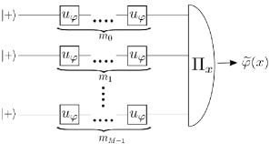
Figure 1: The circuit of a generalized Kitaev’s algorithm. The $i$-th qubit receives the phase shift $m_{i}\varphi$, while the total number of used gates is $\sum m_{i}=N$. A general POVM measurement is applied and the results are used to construct the phase estimator.

In the next section we present a generic extension of the Kitaev’s algorithm. The generalization together with the framework for quantifying the estimation performance not only will allow us to analyze the setups from Berry et al. (2009) using the general Bayesian approach, but also will take into account algorithms where the repetition constraints are relaxed. The framework is robust in that, for a given gate configuration, it provides the optimal end measurement and the achieved estimation cost. Using it we analytically derive the upper bounds for $k=2$ and $k=3$, which are in line with the findings in Berry et al. (2009), and compare them with the numerically obtained optimal strategies.

IV Enhanced Kitaev’s algorithm

For a general Kitaev-like strategy parameterized with the vector $\mathbf{m}$, the output state $|\psi_{\varphi}\rangle=U^{\mathbf{m}}_{\varphi}|+\rangle^{\otimes M}$, $\rho_{\varphi}=|\psi_{\varphi}\rangle\langle\psi_{\varphi}|$, reads explicitly

$$|\psi_{\varphi}\rangle=\frac{1}{\sqrt{2^{M}}}\sum_{j=0}^{2^{M}-1}e^{\mathrm{i}n_{\mathbf{m}}(j)\varphi}|j\rangle,$$ (4)

where $|j\rangle=|j_{0}\dots j_{M-1}\rangle$ denotes a state from the computational basis and $n_{\mathbf{m}}(j)=\sum_{i}m_{i}j_{i}$ represents the multiplicity of phase $\varphi$ that is acquired by the state. The above formula may be rewritten in the more appealing form

$$|\psi_{\varphi}\rangle=\frac{1}{\sqrt{2^{M}}}\sum_{n=0}^{N}e^{\mathrm{i}n\varphi}\sqrt{J_{\mathbf{m}}(n)}|n\rangle,$$ (5)

where $J_{\mathbf{m}}(n)=\sum_{j=0}^{2^{M}-1}\delta_{n,n_{\mathbf{m}}(j)}$ corresponds to the number of basis vectors that evolve with a given phase multiplicity $n$, while

$$|n\rangle=\frac{1}{\sqrt{J_{\mathbf{m}}(n)}}\sum_{j=0}^{2^{M}-1}\delta_{n,n_{\mathbf{m}}(j)}|j\rangle$$ (6)

is the normalized equally weighted superposition of these vectors. Plugging Eq. (5) into Eq. (2) and performing the integration we arrive at the formula for the average cost,

$$\begin{split}\Delta^{2}\varphi_{\mathbf{m}}&=\frac{1}{2^{M-1}}\Big{(}\sum_{n=0}^{N}J_{\mathbf{m}}(n)\Pi_{n,n}+\\ &-\sum_{n=0}^{N-1}\Pi_{n,n+1}\sqrt{J_{\mathbf{m}}(n)J_{\mathbf{m}}(n+1)}\Big{)},\end{split}$$ (7)

where $\Pi_{n,m}=\langle n|\Pi|m\rangle$. The completeness condition $\int U^{\mathbf{m}}_{\varphi}\Pi U^{\mathbf{m}\dagger}_{\varphi}\frac{\textrm{d}\varphi}{2\pi}=\openone$ implies $\Pi_{n,n}=1$, while the positivity constraint $\Pi\geq 0$ implies that $|\Pi_{n,m}|\leq\sqrt{\Pi_{n,n}\Pi_{m,m}}=1$. Hence, the optimal choice for the seed operator $\Pi$, which minimizes $\Delta^{2}\varphi$ in Eq. (7), corresponds to the choice $\Pi_{n,m}=1$. Vectors $\{|n\rangle\}$ do not, in general, span the whole $2^{M}$-dimensional Hilbert space, so the explicit form of the optimal seed operator $\Pi$ reads

$$\Pi=\sum_{n,m}|n\rangle\langle m|+\openone_{\bot},$$ (8)

where $\openone_{\bot}$ represents the identity operator on the subspace orthogonal to the one spanned by $\{|n\rangle\}$. This allows us to produce the set of POVMs $\{\Pi_{\varphi}\}$ parameterized by the continuous index $\varphi$, which, if required, can also be replaced with a finite number of operators Derka et al. (1998); van Dam et al. (2007). The resulting minimal cost reads

$$\Delta^{2}\varphi_{\mathbf{m}}=2-\frac{1}{2^{M-1}}\sum\limits_{n=0}^{N-1}\sqrt{J_{\mathbf{m}}(n)J_{\mathbf{m}}(n+1)}.$$ (9)

From the above formula it readily follows that for the standard Kitaev’s algorithm, parameterized by $\mathbf{m}=\mathbf{m}_{1}$ where $m_{i}=2^{i}$, we have $N=2^{M}-1$ and $J_{\mathbf{m}_{1}}(n)=1$, which results in

$$\Delta^{2}\varphi_{\mathbf{m}_{1}}=2-\frac{2^{M}-1}{2^{M-1}}=\frac{1}{2^{M-1}}=\frac{2}{N+1}.$$ (10)

Hence, as mentioned before, the strategy offers no advantage over the basic parallel product-state-based strategy.

Let us now focus on two more interesting cases, $\mathbf{m}_{2}=\mathbf{m}_{1}\wedge\mathbf{m}_{1}$ and $\mathbf{m}_{3}=\mathbf{m}_{1}\wedge\mathbf{m}_{1}\wedge\mathbf{m}_{1}$, where $\wedge$ denotes vector concatenation. The cases are extensions of the original Kitaev’s algorithm, where each of the $u_{\varphi}^{2^{i}}$ phase shifts is applied to two or three different qubits, respectively. Using Eq. (9) it is possible to obtain analytical bounds on the achievable precision in terms of the total consumed resources $N$ for these two cases, whose derivations are described in more detail in the Appendix, and read

$$\Delta^{2}\varphi_{\mathbf{m}_{2}}\leq 4\frac{\ln(N+2)-\ln 2+3}{(N+2)^{2}}=O\left(\frac{\log N}{N^{2}}\right),$$ (11)

$$\Delta^{2}\varphi_{\mathbf{m}_{3}}\leq\frac{27}{(N+3)^{2}}\frac{N+1}{N+3}=O\left(\frac{1}{N^{2}}\right).$$ (12)

This shows that our estimation costs in these two simple extensions of Kitaev’s algorithm are asymptotically equivalent to those presented in Berry et al. (2009).

V Cost analysis

The upper bounds in the previous section were derived using simple inequalities between means, which raises the question how much more efficient the estimation costs actually are. It would also be insightful to find out how much improvement can be gained by allowing more general gate configurations. In order to address these problems to some extent, numerical simulations for tractable space sizes were carried out. For a given $\mathbf{m}$, the corresponding $J_{\mathbf{m}}(n)$ were calculated, which in turn allowed us to compute the estimation cost using (9). In order to cut down on computation time, only a subspace of nondecreasing vectors $\mathbf{m}$ was considered. We constrained the problem by allowing only powers of 2 as multiplicities. We looked into cases where $M\leq 32$. To further cut down on computation time we enforced at least two repetitions of each multiplicity for $M\in[21,25]$ and at least three for $M\in[26,32]$. The outcomes were then aggregated with respect to $N=\sum m_{i}$ and the lowest cost was stored as the best result found.

The results are presented in Fig. 2. They are compared with the optimal cost given by (3) and a shot-noise benchmark obtained using $\mathbf{m}=\mathbf{m}_{\otimes}$, where $m_{i}=1$, which mimics a classical experiment with repeated estimation using single passes through a $u_{\varphi}$ gate. The numerically obtained cost values for resource numbers $N$ are indeed visibly lower than the analytical bounds, although the asymptotic behavior seems to be preserved.

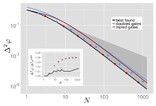
Figure 2: Plot showing the estimation costs with respect to the number of used resources. The black line connects the best numerically found solutions. Filled blue (red) circles show the results for $\mathbf{m}_{2}$ ($\mathbf{m}_{3}$), while lines are the corresponding analytical upper bounds. The dark-gray ribbon depicts the area between the Bayesian estimation optimum and the shot-noise limit given by $\mathbf{m}_{\otimes}$. Inset: Cost ratios of the best found parameter $\mathbf{m}$ to the Bayesian optimum. Ratios correspond to the costs presented in the main plot.

The costs found by the algorithm are nearly optimal. Even though the general structure of the best $\mathbf{m}$ for an arbitrary $N$ seems contrived, for $\mathbf{m}_{3}$ (filled red circles) the costs are already barely discernible from the Bayesian optimum, which is a new finding. For $\mathbf{m}_{2}$ the computed cost is lower than the corresponding bound, yet visibly worse than the optimum. Under the above conditions we only searched through all viable $\mathbf{m}$ values for $N\leq 20$, however, we obtained consistent results for up to $N=1000$ resources. As shown in the inset in Fig. 2 the found results are worse than the optimum by only less than $2\%$. The slightly saw-like shape of the ratios stems from the constraints on $\mathbf{m}$. The value of $\Delta^{2}\varphi/\Delta^{2}\varphi^{\textrm{opt}}$ for $\mathbf{m}_{3}$ was also computed for $N\leq 10^{5}$ and it seems to converge around $1.04$. Our algorithm enhancement can thus deliver estimation costs within a very few percent of the optimum.

VI Setup with photon losses

The efficiency of quantum measurements and algorithms is highly dependent on external noise factors. In this article we focus on one particular noise model, namely, photon losses. The topic has been considered in previous works Kolodyński and Demkowicz-Dobrzański (2010); Knysh et al. (2011); Demkowicz-Dobrzański (2010); Escher et al. (2011); Demkowicz-Dobrzanski and Maccone (2014); Jarzyna and Demkowicz-Dobrzanski (2014) and optimal estimation bounds for the most general strategies are known. Here we want to investigate the ultimate performance of Kitaev-like protocols in the presence of losses from the Bayesian perspective. In our analysis we assume that each phase shift gate has probability $\eta$ of functioning correctly. For the repeated $u_{\varphi}^{m}$ gates the success probability decreases exponentially to $\eta^{m}$ and the chances of losing the photon become $1-\eta^{m}$. This is equivalent to modeling $u_{\varphi}$ as a Mach-Zender interferometer with phase delay $\varphi$ and with power transmission equal to $\eta$ in both arms.

It turns out that we can present the costs for the lossy scenario using noiseless cost values. This follows directly from the formula

$$\Delta^{2}\varphi_{\mathbf{m},\eta}=\displaystyle\sum\limits_{\mathbf{n}\in\{0,1\}^{M}}\Delta^{2}\varphi_{\mathbf{m}\mathbf{n}}\prod_{i=0}^{M-1}\eta^{m_{i}n_{i}}(1-\eta^{m_{i}})^{1-n_{i}},$$ (13)

where vector multiplication is element-wise. The cost is simply a weighted average of noiseless costs where the parameter vectors $\mathbf{m}\mathbf{n}$ are obtained by removing dissipated photons from $\mathbf{m}$. Note that a faulty gate eradicates all information about the phase contained in a particular qubit. By intuition it seems natural to expect that the stronger the noise factor, the lower the phase gate multiplicities of optimal circuits will be.

Simulating Eq. (13) would be computationally infeasible for $N>>10$; instead we propose the following approximation. Each $u_{\varphi}^{m}$ gate is a Bernoulli trial with a probability of success equal to $\eta^{m}$. Repeating it $\eta^{-m}$ times will, on average, yield a successful phase windup, as it is the expected number of trials until first success. This translates to a modified resource expense of $N=\sum_{i}\eta^{-m_{i}}m_{i}$. The estimation variance is naturally not exact for a single experiment, but it holds in the regime of numerous repetitions. Note that losing a photon is equivalent to its entering an orthogonal vacuum state, hence we always have information, whether a trial ends in success or failure. The repetitions might require fresh resources; i.e., in the multipass setting additional photons would be required.

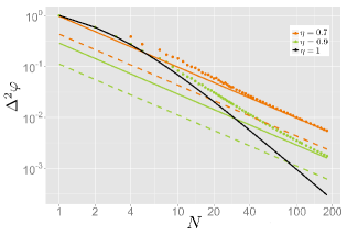
Figure 3: Plot showing the approximate performance of the enhanced Kitaev’s algorithm for two lossy setups. Filled circles reveal the numerically computed cost values of the algorithm, solid lines are the cost limits for entanglement-free strategies, and dashed lines depict the ultimate bounds for the lossy setup where any entangled start states are permitted.

Figure 3 presents the results of numerical simulations for photon losses. Two transmission factors have been considered; the Bayesian noiseless optimum given by Eq. (3) is juxtaposed for comparison. Filled circles depict the numerically found estimation costs, using the same algorithm as in Sec. V, yet with updated resource expenditure. They visibly converge to the solid lines given by

$$\Delta^{2}\varphi_{\eta}^{\mathrm{unentangled}}=\frac{e\ln\left(1/\eta\right)}{N},$$ (14)

which represent the asymptotic optimal cost obtained within the quantum Fisher information approach for unentangled systems Demkowicz-Dobrzanski and Maccone (2014). The convergence of the numerical Bayesian results to the asymptotic cost obtained within the quantum Fisher information approach should be viewed as an illustration of a general claim of asymptotic equivalence of the two approaches in the case where asymptotic scaling of the mean square error is limited to $O(N^{-1})$ Jarzyna and Demkowicz-Dobrzanski (2014). The ultimate bounds (dashed lines), which are valid for any input states including highly entangled ones, are equal to Kolodyński and Demkowicz-Dobrzański (2010); Knysh et al. (2011); Escher et al. (2011); Demkowicz-Dobrzański et al. (2012)

$$\Delta^{2}\varphi_{\eta}^{\mathrm{general}}=\frac{1-\eta}{\eta N}$$ (15)

and are clearly out of reach of the presented strategy. This proves that in the presence of losses, unlike in the decoherence-free case, entanglement is essential for reaching the ultimate precision bound—a fact demonstrated before only within the quantum Fisher information approach Demkowicz-Dobrzański (2010); Demkowicz-Dobrzanski and Maccone (2014).

VII Quantum resources and Shor’s algorithm

The phase estimation procedure is a crucial part of Shor’s algorithm Shor (1997), hence this article would be incomplete if no reference to the famous factorization algorithm were made. Unfortunately, as promptly shown, the proposed enhancements to the phase-estimation algorithm, while useful from the metrological perspective, are of little use from the computational point of view. We do not discuss the whole of Shor’s algorithm, as it is available in the original article and in other works Nielsen and Chuang (2000); Ekert and Jozsa (1996) with detailed examples; we only touch on the parts of the procedure which directly relate to our subject.

The core of Shor’s algorithm is the subroutine for order finding. The task is as follows: given integers $x$ and $N$, $x<N$, we are to find the smallest positive integer $r$ such that $x^{r}\equiv 1\ (\textrm{mod }N)$. This problem is equivalent to factorizing $N$ in the sense that, with an additional expense of polynomial (classical) computation time, we can obtain the solution of one using the other. To embed order finding in the phase estimation setting we utilize the following gate: $u_{x}|y\rangle=|xy\mod N\rangle$. Regardless of the value of $x$ the operator has eigenstates $|e_{s}\rangle,s\in\{0,1,\dots,r-1\}$, where

$$u_{x}|e_{s}\rangle=e^{\frac{\mathrm{i}2\pi s}{r}}|e_{s}\rangle.$$ (16)

By employing Kitaev’s algorithm with $u_{x}$ as the phase imprinting gate (with $x$ selected randomly) and further quantum-mechanical and number-theoretic transformations the algorithm produces $r$ with a high probability.

The intrinsic structure of operator $u_{x}$ underpins the computational power of the algorithm in that we have $u_{x}^{m}=u_{x^{m}\textrm{ mod }N}$. Hence the sequences of controlled $u_{x}^{2^{i}}$ gates can be implemented in the time polynomial with respect to $L=\lceil\log(N)\rceil$ using modular exponentiation. We juxtapose this case with general phase estimation as discussed in earlier sections. Previously we assumed the expense of utilizing a gate $u_{\varphi}^{m}$ to be $m$ (e.g., $m$ photon passes). Here, operating gate $u_{x}^{m}$ will still cost us 1, plus the additional computation time to obtain $x^{m}\mod N$. Using the standard “elementary” multiplication algorithm and modular exponentiation we can perform this computation in time $O\left(L^{2}\log m\right)$, which can also be bounded by $O\left(L^{3}\right)$. We see that in this case a gate $u_{x}^{m}$ can be implemented with a single resource unit, regardless of $m$, and at the cost of computation, whose time is bounded by a constant for a set value of $L$. The approach with repeating gates with lower phase multiplication factors would be counter-productive here.

To conclude this section we remark that when we equate physical resources with the number of qubits $M$ involved, irrespective of the multiplicity of the phase shifts they experience, that is, set $N:=M$, then the original Kitaev’s algorithm parameterized by $\mathbf{m}_{1}$ is indeed the optimal one in terms of cost in the Bayesian approach, and it is also the only optimal solution. A proof of this statement is easily obtained as follows. We assume without loss of generality that $m_{i}>0$. Then $J_{\mathbf{m}}(0)=J_{\mathbf{m}}(N)=1$, and again applying the inequality between the arithmetic and the geometric mean to Eq. (9) and using $\sum_{n}J_{\mathbf{m}}(n)=2^{M}$, we obtain $\forall_{\mathbf{m}}\Delta^{2}\varphi_{\mathbf{m}}\geq\Delta^{2}\varphi_{\mathbf{m}_{1}}$. We have equality iff $J_{\mathbf{m}}(n)=1$, which is only true when $\mathbf{m}=\mathbf{m}_{1}$.

VIII Conclusions

We have found that Kitaev’s phase-estimation algorithm can be naturally generalized to reach optimality in the sense of the Bayesian estimation theory. The enhancement is based on repeated applications of the phase gates and does not require entanglement, although it makes use of general measurements, whose experimental implementation may still pose a challenge. We introduced a framework for analyzing generalizations of Kitaev’s algorithm with the ready-to-use recipe for calculating their costs. We then rederived the analytical bounds first presented in Berry et al. (2009) for Kitaev’s algorithm with doubled and tripled gates. For moderate resource numbers we found algorithm enhancements which approach closely the Bayesian estimation optimum. The behavior of our algorithm was also analyzed in a setup with photon losses where it was shown that they cannot match the performance of the optimal entanglement-based strategies. We have also confirmed the asymptotic equivalence of Bayesian and quantum Fisher information approaches in the problem analyzed. Finally, we considered the enhancement from the point of view of Shor’s factorization procedure. A negative conclusion was reached as to its usefulness for this purpose and the original Kitaev’s algorithm was found to be the only optimal solution, thus revealing an interesting side to the understanding of quantum resources and their utilization in various measurement schemes, including quantum algorithms.

Appendix: Derivation of estimation bounds for doubled and tripled gates

In this section we give examples of how Eq. (9) can be used to obtain costs for various generalizations of Kitaev’s algorithm. Earlier we calculated the cost for $\mathbf{m}_{1}$; here we investigate the cases of $\mathbf{m}_{2}$ and $\mathbf{m}_{3}$, which are of interest from the point of view of this article. Before we do so, however, we take a brief look at what happens when $\mathbf{m}=\mathbf{m}_{\otimes}$; this corresponds to the tensor product of single-qubit phase shift gates, which we have used as a “classical” benchmark before. Using our framework and noting that $J_{\mathbf{m}_{\otimes}}(n)=\binom{N}{n}$ we obtain the cost $\Delta^{2}\varphi_{\mathbf{m}_{\otimes}}$, which, as expected, can be shown to approach $N^{-1}$ for large $N$.

The key to making practical use of Eq. (9) is finding the structure of $J_{\mathbf{m}}(n)$. It is the number of vectors evolving at phase multiplicity $n\varphi$ and also the number of representations of $n$ in a positional system given by $\mathbf{m}$. For $\mathbf{m}_{2}$ it is a “pseudobinary” system where each position is repeated twice. The function can be written in the following recursive form for $0\leq n<2^{\frac{M}{2}}$:

$$J_{\mathbf{m}_{2}}(n)=\left\{\begin{array}[]{ll}J_{\mathbf{m}_{2}}\left(\frac{n}{2}\right)+J_{\mathbf{m}_{2}}\left(\frac{n-2}{2}\right)&:2\mid n\\ 2J_{\mathbf{m}_{2}}\left(\frac{n-1}{2}\right)&:2\centernot\mid n\end{array}\right..$$ (17)

For even $n$ all valid representations either have 0’s at the two least significant bits (of our modified positional system) or have them both set to 1 and use the remainder to represent $n-2$. If $n$ is odd, we have to set exactly one of the two least significant bits, while the rest represent $n-1$. In both cases we can equivalently discard the two fixed bits and look at values shifted to the right by two positions, which is the same as dividing the value by 2. By further noting that $J_{\mathbf{m}_{2}}(0)=1$ we get $J_{\mathbf{m}_{2}}(n)=n+1$ for $0\leq n<2^{\frac{M}{2}}$. On the other hand, for $2^{\frac{M}{2}}\leq n<2^{\frac{M}{2}+1}-1$ the case is analogous when we swap 0’s and 1’s, and we then get $J_{\mathbf{m}_{2}}(n)=J_{\mathbf{m}_{2}}\left(2^{\frac{M}{2}+1}-n-2\right)$.

We can now present the cost formula for $\mathbf{m}_{2}$

$$\Delta^{2}\varphi_{\mathbf{m}_{2}}=2-\frac{1}{2^{M-2}}\sum_{n=0}^{2^{\frac{M}{2}}-1}\sqrt{n(n+1)}.$$ (18)

The sum can be bounded using the inequality between the geometric and the harmonic mean,

$$\sum\limits_{n=0}^{2^{\frac{M}{2}}-1}\sqrt{n(n+1)}\geq\sum\limits_{n=0}^{2^{\frac{M}{2}}-1}\left(n+\frac{n}{2n+1}\right)=2^{M-1}-\frac{1}{2}\sum\limits_{n=0}^{2^{\frac{M}{2}}-1}\frac{1}{2n+1}\geq 2^{M-1}-\frac{1}{4}H(2^{{\frac{M}{2}}})-\frac{1}{2},$$ (19)

where $H(n)$ is the $n$th harmonic number. Using $H(n)\leq\ln n+1$ and setting $N:=2\left(2^{\frac{M}{2}}-1\right)$, we get the bound from Sec. IV.

For $\mathbf{m}_{3}$ the derivation is analogous, although considerably more laborious. The formula, Eq. (9), reads

$$\Delta^{2}\varphi_{\mathbf{m}_{3}}=2-\frac{1}{2^{M-1}}S_{\mathbf{m}_{3}},$$ (20)

where

$$\begin{split}S_{\mathbf{m}_{3}}&=\sum\limits_{k=1}^{2^{{\frac{M}{3}}-1}}(k+1)\sqrt{k(k+2)}+\frac{3}{4}2^{{\frac{2M}{3}}}+\frac{3}{2}\sum\limits_{k=1}^{2^{{\frac{M}{3}}-1}-1}\sqrt{\left(2^{\frac{2M}{3}}-\frac{4k(k-1)}{3}\right)\left(2^{\frac{2M}{3}}-\frac{4k(k+1)}{3}\right)}\\ &\geq 2^{M}-2^{\frac{M}{3}}-\frac{8}{3}\sum\limits_{k=1}^{2^{\frac{M}{3}-1}-1}\frac{k^{2}}{2^{\frac{2M}{3}}-\frac{4k^{2}}{3}}\geq 2^{M}-\frac{3}{2}2^{\frac{M}{3}}+1.\end{split}$$ (21)

Combined with $N:=3\left(2^{\frac{M}{3}}-1\right)$ the above is then easily transformed to Eq. (12).

References

- Giovannetti et al. (2006) V. Giovannetti, S. Lloyd, and L. Maccone, Phys. Rev. Lett. 96, 010401 (2006).
- Giovannetti et al. (2011) V. Giovannetti, S. Lloyd, and L. Maccone, Nature Photonics 5, 222 (2011).
- Abadie et al. (2011) J. Abadie et al. (The LIGO Scientific Collaboration), Nature Phys. 7, 962 (2011).
- Knysh et al. (2011) S. Knysh, V. N. Smelyanskiy, and G. A. Durkin, Phys. Rev. A 83, 021804 (2011).
- Escher et al. (2011) B. Escher, R. de Matos Filho, and L. Davidovich, Nature Physics 7, 406 (2011).
- Demkowicz-Dobrzański et al. (2012) R. Demkowicz-Dobrzański, J. Kołodyński, and M. Guţă, Nat. Commun. 3, 1063 (2012).
- Knysh et al. (2014) S. I. Knysh, E. H. Chen, and G. A. Durkin, ArXiv e-prints (2014), arXiv:1402.0495 [quant-ph] .
- Kolodyński and Demkowicz-Dobrzański (2010) J. Kolodyński and R. Demkowicz-Dobrzański, Phys. Rev. A 82, 053804 (2010).
- Kitaev (1997) A. Y. Kitaev, Russ. Math. Surv. 52, 1191 (1997).
- Shor (1997) P. W. Shor, SIAM journal on computing 26, 1484 (1997).
- Nielsen and Chuang (2000) M. A. Nielsen and I. L. Chuang, Quantum computation and quantum information (Cambridge university press, 2000).
- Higgins et al. (2007) B. L. Higgins, D. W. Berry, S. D. Bartlett, H. M. Wiseman, and G. J. Pryde, Nature 450, 393 (2007).
- Higgins et al. (2009) B. L. Higgins, D. W. Berry, S. D. Bartlett, M. W. Mitchell, H. M. Wiseman, and G. J. Pryde, New Journal of Physics 11, 073023 (2009).
- Berry et al. (2009) D. W. Berry, B. L. Higgins, S. D. Bartlett, M. W. Mitchell, G. J. Pryde, and H. M. Wiseman, Physical Review A 80, 052114 (2009).
- Demkowicz-Dobrzanski and Maccone (2014) R. Demkowicz-Dobrzanski and L. Maccone, ArXiv e-prints (2014), arXiv:1407.2934 [quant-ph] .
- Jarzyna and Demkowicz-Dobrzanski (2014) M. Jarzyna and R. Demkowicz-Dobrzanski, ArXiv e-prints (2014), arXiv:1407.4805 [quant-ph] .
- Holevo (1982) A. S. Holevo, Probabilistic and statistical aspects of quantum theory, Vol. 1 (North-Holland Publishing Company, 1982).
- Chiribella et al. (2004) G. Chiribella, G. M. D’Ariano, P. Perinotti, and M. F. Sacchi, Phys. Rev. A 70, 062105 (2004).
- Berry and Wiseman (2000) D. W. Berry and H. M. Wiseman, Phys. Rev. Lett. 85, 5098 (2000).
- van Dam et al. (2007) W. van Dam, G. M. D’Ariano, A. Ekert, C. Macchiavello, and M. Mosca, Phys. Rev. Lett. 98, 090501 (2007).
- Boixo et al. (2006) S. Boixo, C. M. Caves, A. Datta, and A. Shaji, Laser Physics 16, 1525 (2006).
- Maccone (2013) L. Maccone, Phys. Rev. A 88, 042109 (2013).
- Derka et al. (1998) R. Derka, V. Buzek, and A. K. Ekert, Phys. Rev. Lett. 80, 1571 (1998).
- Demkowicz-Dobrzański (2010) R. Demkowicz-Dobrzański, Laser Physics 20, 1197 (2010).
- Ekert and Jozsa (1996) A. Ekert and R. Jozsa, Rev. Mod. Phys. 68, 733 (1996).