The Black Hole Mass Function Derived from Local Spiral Galaxies

Abstract

We present our determination of the nuclear supermassive black hole mass (SMBH) function for spiral galaxies in the local universe, established from a volume-limited sample consisting of a statistically complete collection of the brightest spiral galaxies in the southern ($\delta<0^{\circ}$) hemisphere. Our SMBH mass function agrees well at the high-mass end with previous values given in the literature. At the low-mass end, inconsistencies exist in previous works that still need to be resolved, but our work is more in line with expectations based on modeling of black hole evolution. This low-mass end of the spectrum is critical to our understanding of the mass function and evolution of black holes since the epoch of maximum quasar activity. A limiting luminosity (redshift-independent) distance, $D_{\rm L}=25.4$ Mpc ($z=0.00572$) and a limiting absolute $B$-band magnitude, $\mathfrak{M}_{\rm B}=-19.12$ define the sample. These limits define a sample of 140 spiral galaxies, with 128 measurable pitch angles to establish the pitch angle distribution for this sample. This pitch angle distribution function may be useful in the study of the morphology of late-type galaxies. We then use an established relationship between the logarithmic spiral arm pitch angle and the mass of the central SMBH in a host galaxy in order to estimate the mass of the 128 respective SMBHs in this volume-limited sample. This result effectively gives us the distribution of mass for SMBHs residing in spiral galaxies over a lookback time, $t_{\rm L}\leq 82.1$ $h_{67.77}^{-1}$ Myr and contained within a comoving volume, $V_{\rm C}=3.37$ $\times$ $10^{4}$ $h_{67.77}^{-3}$ Mpc³. We estimate that the density of SMBHs residing in spiral galaxies in the local universe is $\rho=5.54_{-2.73}^{+6.55}$ $\times$ $10^{4}$ $h_{67.77}^{3}$ $M_{\odot}$ Mpc^-3. Thus, our derived cosmological SMBH mass density for spiral galaxies is $\Omega_{\rm BH}=4.35_{-2.15}^{+5.14}$ $\times$ $10^{-7}$ $h_{67.77}$. Assuming that black holes grow via baryonic accretion, we predict that $0.020_{-0.010}^{+0.023}$ $h_{67.77}^{3}$ $\permil$ of the universal baryonic inventory ($\Omega_{\rm BH}/\omega_{\rm b}$) is confined within nuclear SMBHs at the center of spiral galaxies.

I. Introduction

Strong evidence suggests that supermassive black holes (SMBHs) reside in the nuclei of most galaxies and that correlations exist between the mass of the SMBH and certain properties of the host galaxy (Kormendy & Richstone, 1995; Kormendy & Gebhardt, 2001). It is therefore possible to conduct a census by studying the numerous observable galaxies in our universe in order to estimate demographic information (i.e., mass) for the population of SMBHs in our universe. Following the discovery of quasars (Schmidt, 1963) and the early suspicion that their power sources were in fact SMBHs (Salpeter, 1964; Lynden-Bell, 1969), the study of quasar evolution via quasar luminosity functions (QLFs) has resulted in notable successes in understanding the population of SMBHs in the universe and their mass function. But, studies of the supermassive black hole mass function (BHMF) have left us with no clear consensus, especially at the low-mass end of the spectrum.

It is of particular interest to understand the low-mass end of the BHMF in order to understand how the QLF of past epochs evolves into the BHMF of today (Shankar, 2009). It is now widely accepted that black holes in active galactic nuclei (AGN) do not generally accrete at the Eddington limit (Shankar, 2009). This is not a problem for the brightest and most visible AGN, presumably powered by large black holes accreting at a considerable fraction of their Eddington limit. Smaller black holes cannot imitate this luminosity without accreting at super-Eddington rates. However, one cannot know whether a relatively dim quasar contains a small black hole accreting strongly or a larger black hole accreting at a relatively low rate (a small fraction of its Eddington limit). It is therefore not easy to tell what the BHMF was for AGN in the past, because it is non-trivial to count the number of lower-mass black holes (those with masses in the range of less than a million to ten million solar masses). However, if we counted the number of local lower-mass black holes, the requirement that the BHMF from the quasar epochs evolve into the local BHMF could significantly constrain the BHMF in the past, as well as determine a more complete local picture. Thus, one should pay attention to late-type (spiral) galaxies, since a significant fraction of these lower-mass black holes are found in such galaxies (our own Milky Way being an example).

Some indicators of SMBH mass such as the central stellar velocity dispersion (Gebhardt et al., 2000; Ferrarese & Merritt, 2000) or Sérsic index (Graham & Driver, 2007) have been used to construct BHMFs for early-type galaxies (e.g., Graham et al., 2007). They have been used also to study late-type galaxies, but not always with success because these quantities are defined for the bulge component of galaxies, measuring them in disk galaxies requires decomposition into separate components of the galactic bulge, disk, and bar. Thus, we are currently handicapped in the study of the low-mass end of the BHMF by the relative scarcity of information on the mass function of spiral galaxies. One approach has been to use luminosity or other functions available for all galaxy types in a sample to produce a mass function based upon the relevant scaling relation (Salucci et al., 1999; Aller & Richstone, 2002; Shankar et al., 2004, 2009; Tundo et al., 2007). Our approach contrasts with this one by taking individual measurements of a quantity for each galaxy individually in a carefully selected and complete local sample.

Recently, it has been shown that there is a strong correlation between SMBH mass and spiral arm pitch angle in disk galaxies (Seigar et al., 2008; Berrier et al., 2013). This correlation presents a number of potential advantages for the purposes of developing the BHMF at lower masses. First, there is evidence that it has lower scatter when applied to disk galaxies than any of the other correlations that have been presented (Berrier et al., 2013). Second, the pitch angle is less problematically measured in disk galaxies than the other features, which is likely the explanation for the lower scatter. It does not require any decomposition of the bulge, disk, or bar components besides a trivial exclusion of the central region of the galaxy before the analysis (described below in §II.1). Finally, it can be derived from imaging data alone, which is already available in high quality for many nearby galaxies.

It may be objected that the spiral arm structure of a disk galaxy spans tens of thousands of light years, many orders of magnitude greater than the scale (some few light years) over which the SMBH is the dominating influence at the center of a galaxy. However, as with other correlations of this type, the spiral arm pitch angle does not directly measure the black hole mass, rather it is a measure of the mass of the central region of the galaxy (the bulge in disk-dominated galaxies). The modal density wave theory (Lin & Shu, 1964) describes the spiral arm structure as a standing wave pattern created by density waves propagating through the disk of the galaxy. The density waves are generated by resonances between orbits at certain radii in the disk. As with other standing wave patterns, the wavelength, and therefore the pitch angle of the spiral arms, depends on a ratio of the mass density in the disk to the “tension” provided by the central gravitational well, and thus to the mass of the galaxy’s central region. In the case of spiral density waves in Saturn’s rings, the dependence of the pitch angle on the ratio of the disk mass density to the mass of the central planet has been conclusively shown (Shu, 1984). In galaxies, the central bulge provides (in most cases) the largest part of this central mass. Since it is well known that the mass of the central SMBH correlates with the mass of the central bulge component, it is not at all surprising to find that it also correlates with the spiral arm pitch angle (further details can be found in Berrier et al. 2013).

The pitch angle ($P$) of the spiral arms of a galaxy is inversely proportional to the mass of the central bulge of a galaxy; specifically

$$\cot\left|P\right|\propto M_{\rm Bulge},$$ (1)

where $M_{\rm Bulge}$ is the bulge mass of the galaxy. This is a requirement of all current theories regarding the origin of a spiral structure in galaxies. Since the bulge mass is directly proportional to the velocity dispersion of the bulge via the virial theorem, i.e.,

$$\sigma^{2}\approx\frac{GM_{\rm Bulge}}{R},$$ (2)

where $G$ is the universal gravitational constant and $R$ is the radius of the bulge; and the nuclear SMBH mass is directly proportional to the velocity dispersion via the $M$–$\sigma$ relation, i.e.,

$$M\propto\sigma^{\alpha},$$ (3)

with $\alpha=4.8\pm 0.5$ (Ferrarese & Merritt, 2000); it therefore follows that the mass ($M$) of the nuclear SMBH must be indirectly proportional to the pitch angle of its host galaxy’s spiral arms, i.e.,

$$M\propto 10^{-(0.062\pm 0.009)\left|P\right|},$$ (4)

as shown in Equation (6).

Admittedly, galaxies are complex structures. However, a number of measurable features of disk galaxies are now known to correlate with each other, even though they are measured on very different length scales (e.g., $\sigma$, bulge luminosity, Sérsic Index, and spiral arm pitch angle). Each of these quantities is influenced, or even determined, by the mass of the central bulge of the disk galaxy, and this quantity in turn seems to correlate quite well with the mass of the central black hole. The precise details of how this nexus of what we might call “traits” of the host galaxy correlate to the black hole mass is still subject to debate (see for instance Läsker et al. (2014), which shows that central black hole may correlate equally well with total galaxy luminosity as with central bulge luminosity). Nevertheless, what seems to link the various galaxy “traits” (such as pitch angle, $\sigma$, and so on) is that they are all measures of the mass in the central regions of the galaxy.

That this hidden feature of galaxies, the black hole mass, should be indirectly estimable from measurements of highly visible morphological features, such as pitch angle, is a considerable boon to astronomers. Pitch angle, as a marker for black hole mass, has a number of distinct advantages over other possible markers. It is obtainable from imaging data alone. It is quite unambiguous for many spiral galaxies, whereas other quantities, such as $\sigma$ or Sérsic index, depend upon the astronomer’s ability to disentangle bulge components from bar and disk components. Finally, while $\sigma$ or stellar velocity dispersion depends on the size of the slit used in spectroscopy, with one particular size giving the desired correlation with black hole mass, pitch angle can be considered relatively constant for any annulus-shaped portion of the disk (as long as the spiral arm pattern is truly logarithmic, which is usually the case for all but the very outermost part of the disk). This combination of advantages may permit pitch angle to be used on even larger samples in the future, yielding a better understanding of the evolution of the black hole mass function and its properties in different parts of the universe.

It is worth mentioning the point made by Kormendy et al. (2011); Kormendy & Ho (2013) that the $M$–$\sigma$ relation may not work at all for spiral galaxies with pseudo-bulges rather than classical bulges. This viewpoint has been controversial (e.g., Graham, 2011), but it is born out of the observation that $\sigma$ is defined with “hot” bulges rather than pseudo-bulges in mind in the first place. It can be observed that density wave theory still expects that pitch angle should depend on the central mass of the galaxy, regardless of whether or not the galaxy has a bulge or pseudo-bulge (Roberts et al., 1975). Unfortunately, it is not always trivial to determine which spirals have pseudo-bulges, but it is worth noting that four of the sample used in defining the $M$–$P$ relation in Berrier et al. (2013) are specifically classified by Kormendy et al. (2011) as pseudo-bulges. In addition, Kormendy et al. (2011) feel that a Sérsic index of two can be a good indication that a galaxy has a pseudo-bulge. Berrier et al. (2013) report Sérsic indices for the majority of the galaxies used in their determination of the $M$–$P$ relation and roughly half of them have Sérsic indices less than two. Thus, there are some grounds for expecting that the $M$–$P$ relation may work about as well for pseudo-bulges as for galaxies with classical bulges.

In this paper, we present our determination of the BHMF for local spiral galaxies. We conducted our analysis from a statistically complete sample of local spiral galaxies by measuring their pitch angles using the method of Davis et al. (2012) and use the well-established $M$–$P$ relation (Berrier et al., 2013) to convert the pitch angles ($P$) to SMBH masses ($M$). The paper is outlined as follows. §II discusses the importance of spiral galaxies, our methodology for measuring pitch angles, and presents the $M$–$P$ relation as found by Berrier et al. (2013). §III details our volume-limited sample of spiral galaxies. §IV discusses the results of our pitch angle measurements and their resulting distribution. §V details the conversion of our pitch angle distribution to a black hole mass distribution. §VI reveals our BHMF for spiral galaxies. §VII provides a discussion on the implication of our results. Finally, §VIII contains concluding remarks and a summary of results. We also include in the Appendix, sections discussing the pitch angle of the Golden Spiral (§A), the Milky Way (§B), and listing details of our full sample (§C). Throughout this paper, we adopt a $\Lambda$CDM (Lambda-Cold Dark Matter) cosmology with the best-fit Planck+WP+highL+BAO cosmographic parameters estimated by the Planck mission (Planck Collaboration et al., 2013): $\omega_{\rm b}=0.022161$, $\Omega_{\rm M}=0.3071$, $\Omega_{\Lambda}=0.6914$, and $h_{67.77}=h/0.6777=H_{0}/(67.77$ km s^-1 Mpc${}^{-1})\equiv 1$.

II. Methodology

Our goal of assembling a BHMF for the local universe is accomplished by using pitch angle measurements to estimate black hole masses. Using a well-defined sample, we can construct a representative BHMF. We have completed pitch angle measurements for a volume-limited set of local spiral galaxies, with the aim of ultimately determining the BHMF for the local universe,

$$\frac{\partial{N}}{\partial{M}}=\frac{\partial{N}}{\partial{P}}\frac{\partial{P}}{\partial{M}},$$ (5)

where $N$ is the number of galaxies and $M$ is SMBH mass. The pitch angle measurements for the volume-limited sample give us $\frac{\partial{N}}{\partial{P}}$, while $\frac{\partial{P}}{\partial{M}}$ for spiral galaxies in the local universe has already been discussed and evaluated in the literature (Seigar et al., 2008; Berrier et al., 2013).

II.1. How We Measure Pitch Angle

The best geometric measure for logarithmic spirals is the pitch angle, and this can be measured for any galaxy in which a spiral structure can be discerned, independently of the distance to the galaxy (Davis et al., 2012). We measure galactic logarithmic spiral arm pitch angle by implementing a modified two-dimensional (2D) fast Fourier transform (FFT) software called 2DFFT to decompose charge-coupled device (CCD) images of spiral galaxies into superpositions of logarithmic spirals of different pitch angles and numbers of arms, or harmonic modes ($m$). Galaxies with random inclinations between the plane of their disk and the plane of the sky are deprojected to a face-on orientation. Although Ryden (2004) has argued that disk galaxies are inherently non-circular in outline, their typical ellipticity is not large and, as has been shown by Davis et al. (2012), a small ($\lessapprox 10^{\circ}$ error in inclination angle) departure from circularity does not adversely affect the measurement of the pitch angle. From a user-defined measurement annulus centered on the center of the galaxy, pitch angles are computed for all combinations of measurement annuli, where the inner radius is made to vary by consecutive increasing integer pixel values from zero to one less than the selected outer radius. The pitch angle corresponding to the frequency with the maximum amplitude is captured for the first six non-zero harmonic modes (i.e., for spiral arm patterns containing up to six arms). A mean pitch angle for a galaxy is found by examining the pitch angles measured for different inner radii, selecting a sizable radial region over which the pitch angle is stable. The error depends mostly on the amount of variation in the pitch angle over this selected region. Full details of our methodology for measuring galactic logarithmic spiral arm pitch angle via 2D FFT decomposition can be found in Davis et al. (2012).

II.2. The $M$–$P$ Relation

The pitch angle of a spiral galaxy has been shown to correlate well with the mass of the central SMBH residing in that galaxy (Berrier et al., 2013). Thus, using the linear best-fit $M$–$P$ relation established by Berrier et al. (2013) for local spiral galaxies,

$$\log(M/M_{\odot})=(b\pm\delta b)-(k\pm\delta k)\left|P\right|,$$ (6)

with $b=8.21$, $\delta b=0.16$, $k=0.062$, and $\delta k=0.009$, we can estimate the SMBH masses for a sample of local spiral galaxies merely by measuring their pitch angles using the method of Davis et al. (2012). The linear fit of Berrier et al. (2013) has a reduced $\chi^{2}=4.68$ with a scatter of $0.38$ dex, which is lower than the intrinsic scatter ($\Delta=0.53\pm 0.10$ dex) of the $M$–$\sigma$ relation for late-type galaxies (Gültekin et al., 2009) and the rms residual (0.90 dex) for the SMBH mass–spheroid stellar mass relation for Sérsic galaxies (Scott et al., 2013) in the $\log{M}$ direction. Ultimately, by determining the product of the mass distribution and the pitch angle distribution of a sample with a given volume, we may construct a BHMF for local late-type galaxies.

III. Data

In order to quote a meaningful BHMF, it is first necessary to identify an appropriate sample of host galaxies. We have elected to pursue a volume-limited sample; that is, a population of host galaxies that are contained within a defined volume of space and are brighter than a limiting luminosity. For the sake of defining a statistically complete, magnitude-limited sample, we select southern hemisphere ($\delta<0^{\circ}$) galaxies with a magnitude limit, $B_{\rm T}\leq 12.9$, based on the Carnegie-Irvine Galaxy Survey (CGS); this results in 605 galaxies (Ho et al., 2011). Our sample is selected from galaxies included in the CGS sample, because it is a very complete sample of nearby galaxies for which excellent imaging is freely available (we used a small number of CGS images, whose pitch angles were previously reported in Davis et al. 2012, other images were obtained from the NASA/IPAC Extragalactic Database (NED)). Using this as our parent sample plus the Milky Way gives us a total of 385 spiral galaxies; we then select only spiral galaxies within a volume-limited sample defined by a limiting luminosity (redshift-independent) distance, $D_{\rm L}=25.4$ Mpc ($z=0.00572$) and a limiting absolute $B$-band magnitude, $\mathfrak{M}_{\rm B}=-19.12$ (see Figure 1).

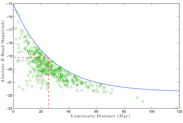
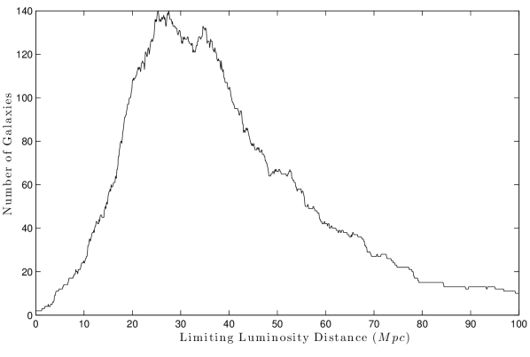
Figure 1.— Top: luminosity distance vs. absolute $B$-band magnitude for all of the spiral galaxies (385) found using the magnitude-limiting selection criteria ($B_{\rm T}\leq 12.9$ and $\delta<0^{\circ}$). The upper limit absolute magnitude can be modeled as an exponential and is plotted here as the solid blue line. The dashed red rectangle is constructed to maximize the number of galaxies in the volume-limited sample. The limiting luminosity distance and absolute $B$-band magnitude are set to be $25.4$ Mpc and $-19.12$, respectively. Bottom: histogram showing the number of galaxies contained in the box in the top panel as the box is allowed to slide to new positions based on the limiting luminosity distance. Note there is a double peak in the histogram maximizing the sample each at 140 galaxies. The two possible combinations are $D_{\rm L}=25.4$ Mpc and $\mathfrak{M}_{\rm B}=-19.12$ or $D_{\rm L}=27.6$ Mpc and $\mathfrak{M}_{\rm B}=-19.33$. We chose to use the former (leftmost peak) because its volume-limiting sample is complete for galaxies with dimmer intrinsic brightness. In total, the two samples differed by only 20 non-mutual galaxies, a difference of $\approx 14\%$. Complete volume-limited samples were computed for limiting luminosity distances ranging from $0.001$ Mpc to $100.000$ Mpc in increments of $0.001$ Mpc.

This results in a volume-limited sample of 140 spiral galaxies within a region of space with a comoving volume, $V_{\rm C}=3.37$ $\times$ $10^{4}$ $h_{67.77}^{-3}$ Mpc³ and a lookback time, $t_{\rm L}\leq 82.1$ $h_{67.77}^{-1}$ Myr. The dimmest (absolute magnitude) and most distant galaxies included in the volume-limited sample are PGC 48179 ($\mathfrak{M}_{\rm B}=-19.12$) and IC 5240 ($D_{\rm L}=25.4$ Mpc), respectively.

In addition, we have determined the luminosity function

$$\phi(\mathfrak{M}_{\rm B})=\frac{\partial{N}}{\partial{\mathfrak{M}_{\rm B}}},$$ (7)

where $N$ is the number of galaxies in the sample for the volume-limited sample in terms of the absolute $B$-band magnitude of each galaxy and dividing by the comoving volume of the volume-limited sample (see Figure 2).

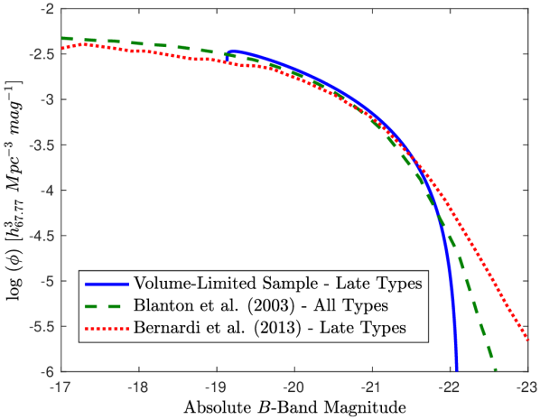
Figure 2.— Luminosity function for the 140 member, volume-limited sample of galaxies obtained from the larger CGS sample. The function is given here (solid blue line) in terms of the probability density function, fit to the results of Equation (7). The function abruptly stops on the dim end due to our exclusion of galaxies with $\mathfrak{M}_{\rm B}>-19.12$. Superimposed for comparison is the $r$-band luminosity functions of $z\approx 0.1$ galaxies selected from the Sloan Digital Sky Survey (SDSS) for all galaxy types (Blanton et al., 2003) and late types (Bernardi et al., 2013); illustrated as green dashed and red dotted lines, respectively. These have all been shifted by $B-r=0.67$ mag, the average color of an Sbc spiral (Fukugita et al., 1995), which is roughly the median Hubble type of both the CGS and our derivative volume-limited sample.

The overall CGS sample has a luminosity function very similar to that found for the much larger Sloan Digital Sky Survey (SDSS) sample (Blanton et al., 2003), indicating that it is a representative sample, in addition to being complete or very near complete. The luminosity function for our sample (a subset of the CGS sample) is shown in Figure 2. Since we imposed a magnitude limit of $\mathfrak{M}_{\rm B}=-19.12$ in order to maintain completeness, our luminosity function does not extend below that limit. Above that limit, our function seems very similar, in outline, to the luminosity function of Blanton et al. (2003) or the late-type galaxies from Bernardi et al. (2013), except for an apparent dearth of spiral galaxies brighter than $\mathfrak{M}_{\rm B}=-22$ in the local universe at distances closer than 25.4 Mpc. Additionally, our selection of the volume-limited sample preserved the distribution of Hubble types in the CGS sample, as shown in Figure 3.

The only notable difference between our luminosity function and that of Blanton et al. (2003) is found at the high-luminosity end, where our function falls off more abruptly. The most likely explanation is that this end of the luminosity function is dominated by a small number of very bright spiral galaxies. It is plausible that the volume in which our sample is found is simply too small to feature a representative number of these relatively uncommon galaxies. This fact is obviously of some relevance to our later analysis of our black hole mass function at the high-mass end, since we would expect very bright spirals to have relatively large black holes.

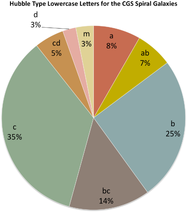
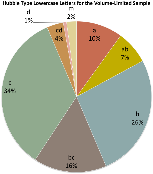
Figure 3.— Top: distribution of the Hubble type subdivisions (lowercase letters) for the 385 spiral galaxies contained in the CGS sample. Bottom: distribution of the Hubble type subdivisions (lowercase letters) for the 140 spiral galaxies contained in the volume-limited subsection of the CGS sample.

We used imaging data taken from various sources as listed in Table LABEL:Sample_Table. Absolute magnitudes were calculated from apparent magnitudes, distance moduli, extinction factors, and $K$-corrections. Only $B$-band absolute magnitudes were used to create a volume-limited sample. For our local sample, the $K$-correction can be neglected. Galactic extinction was determined from the NED Coordinate Transformation & Galactic Extinction Calculator, using the extinctions values for the $B$-band from Schlafly & Finkbeiner (2011).

IV. Pitch Angle Distribution

Pitch angle measurements were attempted for all 140 spiral galaxies in the volume-limited sample according to the method of Davis et al. (2012). However, pitch angles were successfully measured for only 128 of those 140 galaxies ($\approx 91\%$) due to a combination of high inclination angles (10), disturbed morphology due to galaxy-galaxy interaction (1), and bright foreground star contamination (1). Overall, we achieved good coverage of the southern celestial hemisphere with our measurements (see Figure 4)

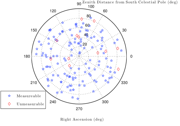
Figure 4.— Location of galaxies on the southern celestial hemisphere. Galaxies with measurable pitch angles are marked with blue stars and galaxies with unmeasurable pitch angles are marked with red diamonds.

and the unmeasurable galaxies are randomly distributed across the southern sky. Since galaxies must first be deprojected to a face-on orientation before their pitch angle can be measured, it becomes increasingly difficult to measure galaxies where the plane of the galaxy is inclined significantly with respect to the plane of the sky. For edge-on galaxies and galaxies with extreme inclinations, it becomes impossible to recover the hidden spiral structure that is angled away from our point-of-view. Additionally, it becomes difficult to resolve spiral arms for low-surface brightness galaxies and galaxies which are too flocculent to ascertain definable spiral arms, although we avoided the former problem by deliberately excluding the dimmest galaxies from our volume-limited sample.

All measured data for individual galaxies included in the volume-limited sample are listed in Table LABEL:Sample_Table. Approximately $55\%$ of the measurable galaxies in the volume-limited sample are observed to have positive pitch angles or clockwise chirality, with the radius of the spiral arms increasing as $\theta\to\infty$ (negative pitch angle implies counterclockwise chirality, with the radius of the spiral arms increasing as $\theta\to-\infty$). This is as expected due to the fact the sign of the pitch angle is merely a line-of-sight effect and thus, should be evenly distributed. Concerning the harmonic modes (see Figure 5),

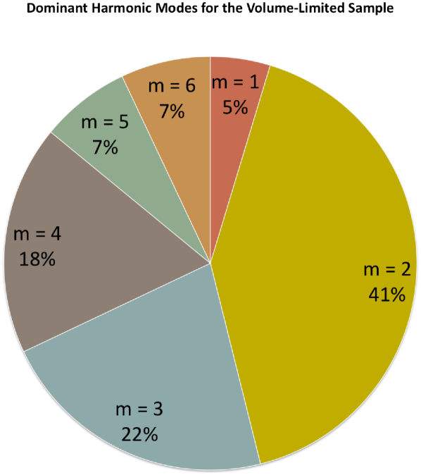
Figure 5.— Dominant harmonic modes ($m$) resulting from the number of spiral arms yielding the highest stability in the resulting pitch angles measured by the 2DFFT software for the sample of 128 measurable spiral galaxies from the volume-limited sample.

the $m=2$ mode (two-armed spirals) was the most common mode ($41\%$) and the even modes constituted the majority ($66\%$). The average error on pitch angle measurements is $\pm 4.81^{\circ}$.

NGC 5792 has the highest inclination angle amongst the galaxies with measurable pitch angles from the volume-limited sample, with an inclination angle $i=80.44^{\circ}$ with respect to the plane of the sky. It is important to note that this is an extreme case, and that pitch angle recovery is usually not possible for galaxies with this inclination. Only galaxies with very high resolution images, like NGC 5792, can hope to have their pitch angles determined when they are so highly inclined. Usually, a more reasonable inclination limit is $i\lessapprox 60^{\circ}$ for galaxies with average or less than average resolution. Using NGC 5792’s inclination angle as a predictor of measurable inclined galaxies, the percentage of randomly inclined galaxies that would satisfy $i\leq 80.44^{\circ}$ is $\approx 89\%$. This is very similar to the percentage of the volume-limited sample that we were able to measure. Of the unmeasurable 12 galaxies, 10 were too highly inclined to measure, 1 galaxy (NGC 275) was overly disturbed due to galaxy-galaxy interaction, and 1 galaxy (NGC 988) was blocked by a very bright foreground star. Due to the random nature of the unmeasurable galaxies, we still consider our volume-limited sample analysis to be statistically complete.

In an effort to minimize the effect of Eddington bias (Eddington, 1913) on our data as a result of binning, we have created a nominally “binless” pitch angle distribution from our sample of 128 galaxies, each with their individual associated errors in measurement (see Figure 6).

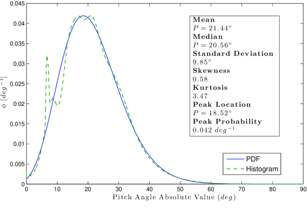
Figure 6.— Pitch angle distribution (dashed green line) and a probability density function (PDF; solid blue line) fit to the data. The pitch angle distribution is a “binless” histogram that we modeled by allowing each data point to be a Gaussian, where the pitch angle absolute value is the mean and the error bar is the standard deviation. The pitch angle distribution is then the normalized sum of all the Gaussians. The resulting PDF is defined by $\mu=21.44^{\circ}$, ${\rm median}=20.56^{\circ}$, $\sigma=9.85^{\circ}$, ${\rm skewness}=0.58$, ${\rm kurtosis}=3.47$, and a most probable pitch angle absolute value of $18.52^{\circ}$ with a probability density value of $\phi=0.042$ deg^-1.

To do this, we constructed a routine to model each data point as a normalized Gaussian, where the pitch angle absolute value is the mean and the error bar is the standard deviation. Subsequently, the pitch angle distribution is then the normalized sum of all the Gaussians. From the resulting pitch angle distribution, we were able to compute the statistical standardized moments of a probability distribution; mean ($\mu$), variance ($\sigma^{2}$, quoted here by means of its square root, $\sigma$, the standard deviation), skewness, and kurtosis by analyzing the distribution with bin widths equal to the maximum resolution of our pitch angle software, $0.01^{\circ}$. Furthermore, the dimensions of the derived data array were scaled by a factor of $10^{5}$ to effectively smooth out the data and give the appearance of a “binless” histogram.

In addition, we also fit a probability density function (PDF) to the pitch angle distribution, according to the computational results of the statistical properties of the sample ($\mu=21.44^{\circ}$, ${\rm median}=20.56^{\circ}$, $\sigma=9.85^{\circ}$, ${\rm skewness}=0.58$, and the ${\rm kurtosis}=3.47$). From the skew-kurtotic-normal fit to the data as seen in Figure 6, it is shown that the most probable pitch angle absolute value for a galaxy is $18.52^{\circ}$, with an associated probability density value of $\phi=0.042$ deg^-1. It is interesting to note that the most probable pitch angle is within $1.5^{\circ}$ of the pitch angle ($\left|P\right|\approx 17.03^{\circ}$) of the Golden Spiral (see Appendix A) and close to the pitch angle ($\left|P\right|=22.5^{\circ}\pm 2.5^{\circ}$) of the Milky Way (see Appendix B). The Milky Way is a better representative of the mean pitch angle of the distribution, being only slightly greater than one degree different.

V. Black Hole Mass Distribution

The measured pitch angle values (Table LABEL:Sample_Table, Column 8) were converted to SMBH mass estimates (Table LABEL:Sample_Table, Column 11) via Equation (6) with fully independent errors propagated as follows:

$$\delta\log(M/M_{\odot})=\sqrt{(\delta b)^{2}+(kP)^{2}[(\frac{\delta k}{k})^{2}+(\frac{\delta P}{P})^{2}]},$$ (8)

where $\delta P$ is the error associated with the pitch angle measurement. Following the procedure for creating the pitch angle distribution (see §IV), we produced a similar black hole mass distribution of the masses listed in Column 11 of Table LABEL:Sample_Table and fit a PDF to the data (see Figure 7).

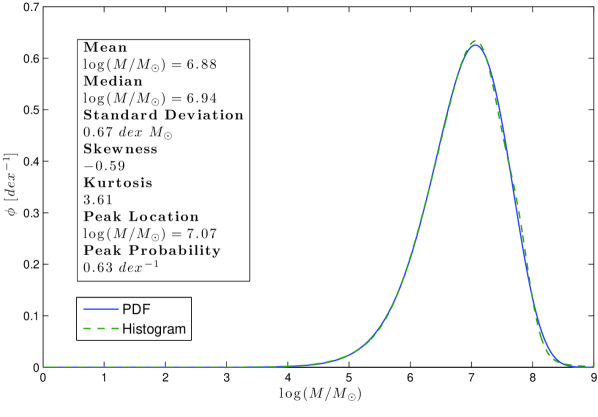
Figure 7.— Black hole mass distribution (dashed green line) and a PDF (solid blue line) fit to the data. The black hole mass distribution is a “binless” histogram that we modeled by allowing each data point to be a Gaussian, where the black hole mass (converted from pitch angle measurements via Equation (6)) is the mean and the error bar is the standard deviation. The black hole mass distribution is then the normalized sum of all the Gaussians. The resulting PDF is defined by $\mu=6.88$ dex $M_{\odot}$, ${\rm median}=6.94$ dex $M_{\odot}$, $\sigma=0.67$ dex $M_{\odot}$, ${\rm skewness}=-0.59$, ${\rm kurtosis}=3.61$, and a most probable SMBH mass of $\log(M/M_{\odot})=7.07$ with a probability density value of $\phi=0.63$ dex^-1.

The resulting PDF, in terms of SMBH mass, is defined by $\mu=6.88$ dex $M_{\odot}$, ${\rm median}=6.94$ dex $M_{\odot}$, $\sigma=0.67$ dex $M_{\odot}$, ${\rm skewness}=-0.59$, ${\rm kurtosis}=3.61$, and a most probable SMBH mass of $\log(M/M_{\odot})=7.07$ with a probability density value of $\phi=0.63$ dex^-1. Conversion to mass has effectively smoothed out the previous pitch angle distribution (see Figure 6), and produced a slightly more pointed (higher kurtosis) distribution. This smoothing is due to propagation of errors through Equation (6), with its errors in slope and $Y$-intercept, leading to wider individual Gaussians assigned to each measurement with subsequent summation to form the black hole mass distribution in Figure 7.

Nine galaxies in the sample have independently estimated SMBH masses from the literature (see Table V) and were included in the construction of the $M$–$P$ relation of Berrier et al. (2013). Rather than using these masses in our black hole mass distribution or subsequent BHMF, we chose to consistently use masses determined from the $M$–$P$ relation defined by Berrier et al. (2013). Our estimated masses agree with the measured masses within the listed uncertainties in all cases, as shown in Table V. This is not surprising given that they are included in the Berrier et al. (2013) sample, which is defined by the directly measured masses of these galaxies (amongst others).

Table 1Black Hole Masses from Independent Literature Sources

	This Work		Literature
Galaxy Name	$\log(M/M_{\odot})$		$\log(M/M_{\odot})$	Method	Reference
(1)	(2)		(3)	(4)	(5)
ESO 097-G013	$6.55\pm 0.42$		$6.23_{-0.08}^{+0.07}$	1	1
Milky Way	$6.82\pm 0.30$		$6.63\pm 0.04$	2	2
NGC 253	$6.92\pm 0.54$		$\approx 6.94$	1	3
NGC 1068	$6.93\pm 0.37$		$6.88\pm 0.02$	1	4
NGC 1300	$7.42\pm 0.23$		$7.80\pm 0.29$	3	5
NGC 1353	$7.36\pm 0.25$		$6.64\pm 0.71$	4	6
NGC 1357	$7.21\pm 0.31$		$7.19\pm 0.71$	4	6
NGC 3621	$7.43\pm 0.21$		$\gtrapprox 3.64$	5	7
NGC 7582	$7.30\pm 0.51$		$7.75_{-0.18}^{+0.17}$	3	8

Note. — Columns: (1) Galaxy name (in order of increasing R.A.). (2) SMBH mass in $\log(M/M_{\odot})$, converted from the pitch angle by Equation (6). (3) SMBH mass in $\log(M/M_{\odot})$, as listed by independent literature sources (when applicable, masses have been adjusted to conform with our defined cosmology). (4) SMBH mass estimation method used by independent literature source. (5) Literature source of SMBH mass. Method: (1) ${\rm H_{2}O}$ maser; (2) stellar orbits; (3) gas dynamics; (4) $M$–$\sigma$ relation; (5) Eddington limit.

References. — (1) Greenhill et al. (2003); (2) Levine et al. (2006); (3) Rodríguez-Rico et al. (2006); (4) Lodato & Bertin (2003); (5) Atkinson et al. (2005); (6) Ferrarese (2002); (7) Satyapal et al. (2007); (8) Wold et al. (2006).

It is also worth noting that half a dozen galaxies included in our volume-limited sample harbor nuclear star clusters (NSC) with well-determined masses (Erwin & Gadotti, 2012). The existence of a NSC in a galaxy does not rule out the coexistence of a SMBH and vice versa. For instance, the Milky Way and M31 have been shown to both contain a NSC and a SMBH, all with well-determined masses (Erwin & Gadotti, 2012). It has been shown that NSCs and SMBHs do not follow the same host-galaxy correlations; SMBH mass correlates with the stellar mass of the bulge component of galaxies, while NSC mass correlates much better with the total galaxy stellar mass (Erwin & Gadotti, 2012). Because of this, our implied SMBH masses for these seven galaxies is not equivalent to the known masses of their NSCs, their only known central massive objects (see Table V). By comparing the central massive objects in Table V, it can be seen that the average NSC mass is higher than the average SMBH mass for this sample; $\log(M/M_{\odot})=7.55\pm 0.16$ and $\log(M/M_{\odot})=7.04_{-0.25}^{+0.28}$, respectively.

Table 2Galaxies with Well-determined NSC Masses

	SMBHs		NSCs
Galaxy Name	$\log(M/M_{\odot})$		$\log(M/M_{\odot})$		Reference
(1)	(2)		(3)		(4)
Milky Way	$6.82\pm 0.30$		$7.48_{-0.30}^{+0.18}$		1
NGC 1325	$7.35\pm 0.21$		$7.12\pm 0.30$		2
NGC 1385	$5.99\pm 0.49$		$6.30\pm 0.30$		2
NGC 3621	$7.43\pm 0.21$		$\approx 7.01$		3
NGC 4030	$6.75\pm 0.44$		$8.05\pm 0.30$		2
NGC 7418	$6.58\pm 0.59$		$7.75\pm 0.19$		4

Note. — Columns: (1) Galaxy name. (2) SMBH mass in $\log(M/M_{\odot})$, converted from the pitch angle by Equation (6). (3) NSC mass in $\log(M/M_{\odot})$. (4) Source of NSC measurement.

References. — (1) Launhardt et al. (2002); (2) Rossa et al. (2006); (3) Barth et al. (2009); (4) Walcher et al. (2005).

Ultimately, Figure 7 provides us with a look at a simple 1:1 conversion from pitch angle to SMBH mass via the $M$–$P$ relation. Since this only applies to the 128 measurable galaxies (out of the total volume-limited sample of 140 galaxies), it offers the most direct look at the distribution of SMBH masses in the Local Universe. The subsequent section will extend the results into the complete BHMF via extrapolation to the full 140 member volume-limited sample and full treatment of sampling from probability distributions.

VI. Black Hole Mass Function for Local Spiral Galaxies

The pitch angle function $\phi(P)$ is defined as

$$\phi(P)=\frac{\partial{N}}{\partial{P}},$$ (9)

where $\phi(P)dP$ is defined to be the number of galaxies that have pitch angles between $P$ and $P+dP$. That should be $\frac{\partial{N}}{\partial{P}}dP$ because

$$N=\int_{0}^{\pi}\frac{\partial{n}}{\partial{P}}dP$$ (10)

is the total number of galaxies in the sample. Then the BHMF is

$$\phi(M)=\frac{\partial{N}}{\partial{M}}=\frac{\partial{N}}{\partial{P}}\frac{\partial{P}}{\partial{M}}=\phi(P)\frac{\partial{P}}{\partial{M}}.$$ (11)

Therefore, by taking the derivative of Equation (6) we find

$$\frac{1}{M\ln(10)}=-(k\pm\delta k)\frac{\partial{P}}{\partial{M}}$$ (12)

or

$$\frac{\partial{P}}{\partial{M}}=-\frac{1}{M\ln(10)(k\pm\delta k)}.$$ (13)

Therefore,

$$\phi(M)=-\frac{\phi(P)}{M\ln(10)(k\pm\delta k)}.$$ (14)

Alternatively, we could calculate

$$\phi(\log M)=\frac{\partial{N}}{\partial{\log M}}=\frac{\partial{N}}{\partial{P}}\frac{\partial{P}}{\partial{\log M}}=-\frac{\phi(P)}{k\pm\delta k}.$$ (15)

Through the implementation of Equation (15) and dividing by the comoving volume of the volume-limited sample ($V_{\rm C}=3.37$ $\times$ $10^{4}$ $h_{67.77}^{-3}$ Mpc³), the pitch angle PDF in Figure 6 can be transformed into a BHMF. Using the probabilities established by the PDF in Figure 6, we can predict probable masses for the remaining 12 unmeasurable galaxies in the volume-limited sample, in order to extrapolate the BHMF and related parameters for the full sample size. The evaluation of BHMF with the summation of all SMBH masses and total densities for both the measurable sample of 128 SMBHs and the extrapolated full volume-limited sample of 140 SMBHs are listed in Table 3.

Table 3Black Hole Mass Function Evaluation

N	$M_{\rm Total}$	$\rho$	$\Omega_{\rm BH}$	$\Omega_{\rm BH}/\omega_{\rm b}$
	($10^{9}$ $M_{\odot}$)	($10^{4}$ $h_{67.77}^{3}$ $M_{\odot}$ Mpc-3)	($10^{-7}$ $h_{67.77}$)	($h_{67.77}^{3}$ $\permil$)
(1)	(2)	(3)	(4)	(5)
128	$1.75_{-0.85}^{+2.05}$	$5.17_{-2.52}^{+6.07}$	$4.06_{-1.98}^{+4.76}$	$0.018_{-0.009}^{+0.022}$
140	$1.87_{-0.92}^{+2.21}$	$5.54_{-2.73}^{+6.55}$	$4.35_{-2.15}^{+5.14}$	$0.020_{-0.010}^{+0.023}$

Note. — Columns: (1) Number of galaxies (measurable 128 SMBHs or an extrapolation for the full volume-limited sample of 140 SMBHs). (2) Total mass from the summation of all the SMBHs in units of $10^{9}$ $M_{\odot}$. (3) Density (Column (2) divided by $3.37$ $\times$ $10^{4}$ $h_{67.77}^{-3}$ Mpc³) of SMBHs in units of $10^{4}$ $h_{67.77}^{3}$ $M_{\odot}$ Mpc^-3. (4) Cosmological SMBH mass density for spiral galaxies ($\Omega_{\rm BH}=\rho/\rho_{0}$), assuming $\rho_{0}\equiv 3H_{0}^{2}/8\pi G=1.274$ $\times$ $10^{11}$ $M_{\odot}$ Mpc^-3 when $H_{0}=67.77$ km s^-1 Mpc^-3. (5) Fraction of the universal baryonic inventory locked up in SMBHs residing in spiral galaxies ($\Omega_{\rm BH}/\omega_{\rm b}$).

In order to determine errors on the calculated late-type BHMF, we ran a Markov Chain Monte Carlo (MCMC) sampling of the late-type BHMF. The sampling consisted of $10^{5}$ realizations for each of the 128 measured galaxies, with pitch angles randomly generated from the data with a Gaussian Distribution within $5\sigma$ of each measured pitch angle value. In addition, the fit to the $M$–$P$ relation (Equation (6)) was also allowed to vary based on the intrinsic errors in slope and $Y$-intercept, which again assumes a Gaussian distribution around the fiducial values. Ultimately, SMBHs are determined from pitch angle values using both the fiducial and randomly adjusted fit. Comparison between the two samples allowed us to represent the fit to the late-type BHMF with error regions. We display the results both as a PDF and a cumulative density function (CDF) fit to the data (see Figure 8).

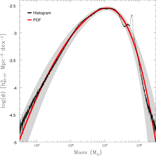
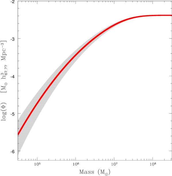
Figure 8.— Top: MCMC sampling of the late-type BHMF (rough black line) with the best fit model PDF (solid red line) surrounded by a $\pm 1\sigma$ error region (gray shading). When integrated, the area under the curve yields the number density for the entire volume-limited sample, 4.15 $\times$ $10^{-3}$ $h_{67.77}^{3}$ Mpc^-3. The plotted data for the top panel is listed for convenience in Table 4. Bottom: MCMC sampling of the late-type BHMF with the best fit model CDF (solid red line) surrounded by a $\pm 1\sigma$ error region (gray shading). The CDF visually depicts the integration of the above PDF in the top panel from $M=0$ until any desired reference point. Here, $\Phi$ is used to indicate an integrated probability, elsewhere $\phi$ is used to indicate a probability density. The upper asymptote approaches the number density for the entire volume-limited sample, 4.15 $\times$ $10^{-3}$ $h_{67.77}^{3}$ Mpc^-3.

The plotted data for Figure 8 (top) is listed for convenience in Table 4. The location of the peak and its value for the MCMC PDF are $\log(M/M_{\odot})=7.07_{-0.09}^{+0.09}$ and $\phi=2.84_{-0.23}^{+0.26}$ $\times$ $10^{-3}$ $h_{67.77}^{3}$ Mpc^-3 dex^-1, respectively. Additionally, we provide a proportional plot for Figure 8 (top), in terms of the product of the BHMF probability density and the SMBH mass ($\phi M$), showing the contribution by the SMBH mass to the cosmic SMBH mass density (see Figure 9).

Table 4BHMF MCMC PDF Values

$\log(M/M_{\odot})$	$\phi$ ($10^{-4}$ $h_{67.77}^{3}$ Mpc-3 dex-1)
(1)	(2)
5.00	$0.65_{-0.36}^{+0.52}$
5.25	$1.38_{-0.67}^{+0.87}$
5.50	$2.74_{-1.14}^{+1.34}$
5.75	$5.01_{-1.72}^{+1.88}$
6.00	$8.46_{-2.33}^{+2.39}$
6.25	$13.19_{-2.82}^{+2.76}$
6.50	$18.92_{-3.01}^{+2.83}$
6.75	$24.67_{-2.83}^{+2.47}$
7.00	$28.23_{-2.58}^{+2.18}$
7.25	$26.53_{-3.02}^{+2.62}$
7.50	$18.90_{-3.21}^{+3.06}$
7.75	$9.49_{-2.91}^{+3.22}$
8.00	$3.19_{-1.77}^{+2.34}$
8.25	$0.69_{-0.58}^{+1.07}$
8.50	$0.09_{-0.09}^{+0.32}$

Note. — Columns: (1) SMBH mass listed as $\log(M/M_{\odot})$ in $0.25$ dex intervals. (2) BHMF number density values from the resulting PDF fit to the MCMC sampling at the given mass in units of $10^{-4}$ $h_{67.77}^{3}$ Mpc^-3 dex^-1.

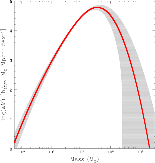
Figure 9.— Contribution by the SMBH mass to the cosmic SMBH mass density (solid red line) surrounded by a $\pm 1\sigma$ error region (gray shading). This plot is proportional to Figure 8 (top), in that this is the product of the BHMF and the SMBH mass ($\phi M$). When integrated, the area under the curve for this plot yields the SMBH mass density, $\rho=5.54_{-2.73}^{+6.55}$ $\times$ $10^{4}$ $h_{67.77}^{3}$ $M_{\odot}$ Mpc^-3.

Since the role played by the intrinsic error in the $M$–$P$ relation is of particular interest, we also adopted the procedure described in (Marconi et al., 2004) (see Equation (3) of that paper and the surrounding discussion) which convolves the distribution function of (in our case) pitch angles in our sample with a Gaussian distribution representing the intrinsic scatter of the $M$–$P$ relation. Since the true intrinsic scatter of this relation is unknown, we simply used the maximum dispersion of 0.38 dex found in (Berrier et al., 2013). In reality, the intrinsic dispersion is presumably somewhat less than this, since at least some of the scatter found in that paper must be due to measurement errors (of both pitch angle and black hole mass). The result of this calculation is a mass function that is broader than that discussed previously because we allow for the possibility that some galaxies are misplaced due to an intrinsic uncertainty in translating from a pitch angle measurement to a black hole mass. The natural result is to broaden the mass function, as compared to one with no intrinsic dispersion assumed. In Figure 10,

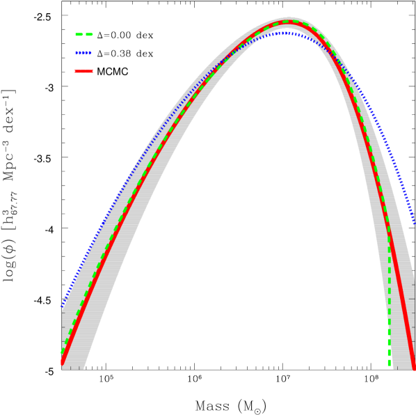
Figure 10.— Comparison of the BHMFs generated through MCMC sampling (solid red line with gray shading) and through convolution of the probabilities associated with zero (dashed green line) and 0.38 dex (dotted blue line) intrinsic dispersions.

we see that on the low-mass side this calculation agrees very well with the outer $1\sigma$ error region from the MCMC calculation. This is not surprising since both the convolution technique and the MCMC calculation account for intrinsic dispersion as well as measurement error in pitch angle. It is evident that the zero intrinsic dispersion BHMF is very similar to the MCMC BHMF, except for the abrupt stop of the zero intrinsic dispersion BHMF at $\log(M/M_{\odot})=8.21$, due to the $Y$-intercept of the $M$–$P$ relation. On the high-mass side, the convolution technique actually broadens the mass function even more and this is significant, as we will see in the next section, in view of comparisons to be made with mass function derived from other techniques.

VII. Discussion

Compared to the attention focused on the early-type mass function, there have been notably less efforts to estimate the local BHMF for spiral or late-type galaxies. Even studies that produce a BHMF for all types of galaxies will often use a different procedure for producing the late-type portion of it. An example is that of Marconi et al. (2004), which uses a velocity dispersion relation for early-type galaxies in the SDSS based on actual measurements of $\sigma$. They include a BHMF for all galaxy types as well, from which one can deduce their late-type BHMF (see Figure 11).

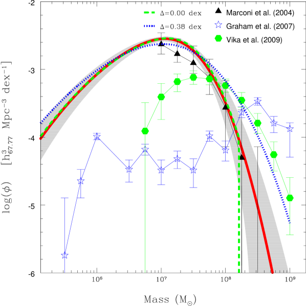
Figure 11.— Comparison between our determination of the BHMF for late-type galaxies with our MCMC fit in red with a gray shaded $\pm 1\sigma$ error region, zero intrinsic dispersion (dashed green line), and 0.38 dex intrinsic dispersion (dotted blue line); with those of Marconi et al. (2004), depicted by black triangles (a late-type BHMF is not provided in Marconi et al. (2004), we have merely subtracted their early-type function from their all-type function); Graham et al. (2007), depicted by blue stars; and Vika et al. (2009), depicted by green hexagons. The BHMF of Vika et al. (2009) is derived using a relationship between SMBH mass and the luminosity of the host galaxy spheroid, applied to a dust-corrected sample of 312 late-type galaxies from the Millennium Galaxy Catalogue in the redshift range $0.013\leq z\leq 0.18$. The peak of our BHMF is located at $\log(M/M_{\odot})=7.06$, whereas theirs is located at $\log(M/M_{\odot})=7.50$. However, Vika et al. (2009) consider BHMF data for $\log(M/M_{\odot})<7.67$ to be unreliable because it is derived from galaxies with $\mathfrak{M}_{\rm B}>-18$, according to their relationship. Note that our entire sample consists of galaxies with $\mathfrak{M}_{\rm B}\leq-19.12$.

Their data for late-type galaxies is based on a velocity dispersion function given by Sheth et al. (2003), who appear to define late types as being spiral galaxies, as we do, including lenticulars with the early types. They make use of the Tully–Fisher relation (Tully & Fisher, 1977) to convert the luminosity function of late types in the SDSS into a function of the circular velocities of these galaxies (meaning that the typical rotational velocity of each of their galactic disks) and then use an observed and expected correlation between these circular velocities and the velocity dispersion ($\sigma$) of their bulges to obtain a velocity dispersion relation for late types. Marconi et al. (2004) then invoke the $M$–$\sigma$ relation to convert this into a BHMF. It is worth noting the number of steps involved in this process and the fact that the final product does not incorporate any data from the SDSS beyond the luminosity function of the galaxies involved. It is obviously encouraging that the results of Marconi et al. (2004) agree so well with our mass function (assuming zero intrinsic dispersion in the $M$–$P$ relation) at the high-mass end (see Figure 11). We cannot compare at the low-mass end, where Marconi et al. (2004) do not provide any data.

In Figure 11, we also compare to the work of Graham et al. (2007), which is based on measurements of the Sérsic index of the galactic bulge. As can be seen in Figure 11, it is difficult to interpret the data of Graham et al. (2007) for late-type galaxies and this may be due to the increased difficulty in extracting Sérsic index values for this type of galaxy, where one must disentangle multiple galactic components (disk and often bar) in order to obtain the Sérsic index (A. Graham 2012, private communication). Our numbers agree far better with those found in Marconi et al. (2004).

An example of more recent work with which we can compare is the late-type BHMF presented in Vika et al. (2009), which is based upon measurements of bulge luminosities in late-type galaxies in the SDSS. Figure 11 also compares our BHMF with theirs. At the very high-mass end our mass function, allowing for the intrinsic dispersion of the $M$–$P$ relation, it comes quite close to the mass function of Vika et al. (2009). At the middle and low-mass end, in contrast, their mass function is far below what we find.

Vika et al. (2009) use the SDSS while our sample is based upon the selection in the CGS, which is considerably more local. Our most distant galaxy has (in our cosmology) a redshift of 0.00572. Their nearest galaxy has a redshift of 0.013 and their most distant is close to $z=0.18$. They have 312 objects in their late-type sample, we have roughly half that. However, the volume of their sample is considerably larger than ours ($\approx 41$ times), so we would expect more late-types in theirs if they were sampling the same types of galaxies as ours. Given that their sample is more distant, it seems likely that they are missing the dimmer galaxies, which would tend to explain the relative scarcity of smaller black holes in their BHMF. On the other hand, their much larger sample volume makes it more likely that they have observed the brighter spirals that may be missing from our sample, based on the luminosity function comparison shown in Figure 2.

Comparing the Vika et al. (2009) late-type mass function with ours (from Figure 11), we are struck overall by the generally good agreement we find. Although there is some disagreement between Marconi et al. (2004) and Vika et al. (2009) at the high-mass end, the comparison with our results sheds some light on a possible reason. We agree very closely with Marconi et al. (2004) when assuming no error in the $M$–$P$ relation, and are quite close to Vika et al. (2009) when we assume that all of the scatter in the $M$–$P$ relation is due to an intrinsic dispersion in that correlation. Since presumably at least some of that scatter is merely due to measurement error in either $M$ or $P$, it is natural to expect that the true SMBH at the high-mass end falls somewhere between the curves given by Marconi et al. (2004) and Vika et al. (2009). It should be kept in mind that the evidence of a deficit in very bright spirals in our volume-limited sample does lend credence to the view that the final result may be close to the line given by Vika et al. (2009) at the very high-mass end. However, in addition, the fact that the high-mass end of the black hole spectrum is dominated by a relatively small number of large objects is one explanation of why a certain level of disagreement is not altogether unexpected in this regime. In short, it looks as if Marconi et al. (2004) and Vika et al. (2009) each fall at opposite limits of our error bars in this regime, which suggests that none of the three results are in severe conflict with each other.

In the low-mass end, there is much less data with which we can compare. Vika et al. (2009) disagree strongly with us on the low-mass end. Their data is based on a sample drawn from the SDSS, which covers a much larger volume of space than our sample, which is based on the most local part of the CGS. In spite of this, Vika et al. (2009) have only twice as many late-type galaxies in their total sample as we do. It seems likely that Vika et al. (2009) miss many galaxies because they are too dim to be easily observed at the greater range of their sample. This could explain the fact that we see far more smaller black holes than they do. Therefore, we conclude that we are not yet in a position to compare with any similarly complete surveys in this particular regime. The good agreement we enjoy with other results at the high-mass end obviously gives grounds for optimism on the low-mass end. We have made a considerable effort to provide a complete local sample precisely because of our interest in producing reliable data on the low-mass end of the black hole spectrum. Obviously, since we have a luminosity cutoff, we must accept that we could be missing black holes at the low-mass end, black holes which would reside in dimmer galaxies and thus might be expected to be relatively small.

We chose to apply our luminosity cutoff firstly for the sake of completeness, because we cannot see many of the dimmer spiral galaxies that must lie in our cosmic neighborhood (see Figure 1). Additionally, we foresee our sample being used to make comparisons with more distant samples, for instance, to study the evolution of the SMBH. It seems likely that those distant samples will not be able to observe these dim galaxies either. Providing a clear luminosity limit may make such comparisons easier. Of course, ultimately we do aim to study the extent to which these dimmer spirals do contribute to the BHMF, but there is an important caveat. It is by no means certain that all such galaxies actually do contain black holes. They have been studied very little and there have been claims that at least some such galaxies do not contain central black holes, but only nuclear star clusters (Ferrarese et al., 2006). For instance, a large majority of the galaxies used to establish the $M$–$P$ relation in (Berrier et al., 2013) had a black hole with mass greater than 6.5 million solar masses (the lowest mass SMBH in the sample use to define the $M$–$P$ relation was found in NGC 4395 with $\log(M/M_{\odot})=5.56_{-0.16}^{+0.12}$), so it clear that the relation is much better constrained at the high-mass end than the low-mass end, as with all other such relations. Caution seems to be warranted in exploring this part of the sample and we pass over it in this paper in the face of such uncertainty.

Ultimately, a total BHMF for all types of galaxies is desired. In Figure 12,

Figure 12.— Visualization of all-type BHMF mass functions generated by the addition of the MCMC PDF of our late-type BHMF with the early-type BHMFs of Marconi et al. (2004), Graham et al. (2007), and Vika et al. (2009) represented by black triangles, blue stars, and green hexagons, respectively.

we add the MCMC PDF of our late-type BHMF to the early-type BHMFs found in Marconi et al. (2004), Vika et al. (2009), and Graham et al. (2007). It is of particular interest to note that all three of these quite varied sources (Marconi et al. 2004 uses $\sigma$, Vika et al. 2009 uses bulge luminosity, and Graham et al. 2007 uses the Sérsic index to derive their BHMFs) agree near the peak of the BHMF, although there are considerable disagreements on the high-mass end. This does suggest that if we could become more confident of the true state of the late-type BHMF, then we would be in a position to have a thorough understanding of the low-mass end of the all-type BHMF.

VIII. Conclusions

Through the application of our established relationship between the mass of central SMBHs and the spiral arm pitch angle of their host galaxies (Berrier et al., 2013), we have been able to establish a robust BHMF for SMBHs residing in spiral galaxies in the local universe. Berrier et al. (2013) demonstrate that the $M$–$P$ relation has the lowest scatter of any method currently used to estimate the mass of SMBHs residing in spiral galaxies. Its strength resides in the relationship being statistically tight, relative ease of implementation, and its independence from cosmographic parameters. We have also ascertained the distribution of pitch angles in the local universe, finding that our Milky Way has a pitch angle slightly higher than the average nearby spiral galaxy. Intriguingly, the discovery that the most probable geometry of spiral arms is close to that of the Golden Spiral was a serendipitous result.

We have now implemented the first major use of the $M$–$P$ relation in this determination. We are encouraged that our estimate of the local mass density of SMBHs in late-type galaxies agrees within order of magnitude with other published values. Our generation of a pitch angle distribution function demonstrates that the most probable mass of a SMBH residing in a spiral galaxy is $\approx 1.16\times 10^{7}M_{\odot}$. This is approximately an order of magnitude less than the most probable mass of a SMBH residing in an early-type galaxy (Marconi et al., 2004). Furthermore, our result is consistent with the current galactic evolutionary construct that galaxies evolve across the Hubble Sequence (Hubble, 1926) from late-type toward early-type galaxies.

The low-mass end of the BHMF presents a number of challenges. Since high-mass black holes are found in more luminous galaxies, they are naturally easier to study since data is easier to acquire. As long as we are interested in local galaxies, this is not an insurmountable obstacle in itself. We have, for the moment, not dealt with the dimmest class of spiral galaxies, for the sake of completeness. Nevertheless, our sample is still peaked at the region (from a million solar masses to 50 million solar masses) that has been identified as the key region within which, if we better understood the local SMBH function, we could learn more about the accretion rates of quasars and AGN in the past. Specifically, it would be possible to constrain the fractions of the Eddington accretion rate at which low-mass or high-mass black holes had accreted in the past (Shankar, 2009).

A natural assumption seen in early work on the continuity equation was that all AGN accrete at the Eddington limit. Convenient though this would be for modern astronomers, there is substantial evidence now that it is untrue. If we could assume that all black holes accrete at the same constant fraction of their Eddington limit, then it would be easy to work out the evolution of the BHMF. This is because each quasar luminosity observed would correspond to a given mass of black hole. One could work out the mass and accretion rate of each black hole and determine at what point in the local BHMF it would ultimately appear. However, more realistically, suppose that there is a random distribution about a mean for each black hole, so that for instance, every black hole accretes at a set fraction of the Eddington limit (the mean of the distribution) plus or minus some random amount (determined by the width of the distribution). Then, it follows that some large black holes will in fact accrete at a relatively small rate. When they do, they can be mistaken for smaller black holes accreting at the normal rate or better for a black hole of that size. The result is that if large black holes often radiate at too small a rate, then we will tend to overestimate the number of small black holes and their rate of accretion. It is hard to tell the difference between large black holes underperforming and small black holes over-performing. One way to check is to count the number of small black holes that actually exist today.

As discussed in the previous section, the quantity and results of studies on the BHMF in spiral galaxies leaves much to be desired. We present ours as of particular interest because it is a complete sample within set limits. As such it may prove easier for future studies to compare their results to ours. Even if they have a broader sample, it should be possible for them to compare with our sample within our known limits. Of the other BHMF’s available for comparison, it is encouraging that we have good agreement, at the high-mass end, with those of Marconi et al. (2004) and Vika et al. (2009). This gives us confidence that our numbers our generally reliable and we argue that we thus have the first dependable estimate of the low-mass end of the spiral galaxy black home mass function. Previous studies of the late-type mass function either have acknowledged problems with spiral galaxies (Graham et al., 2007), do not cover the low-mass end at all (Marconi et al., 2004), or do so with a sample which is likely to suffer strongly from Malmquist bias and be very incomplete for dimmer galaxies (Vika et al., 2009). We hope that our sample will thus be useful to those studying the evolution of the BHMF as a way of constraining the final population of relatively low mass black holes in the universe. One important lesson already stands out. Previous estimates of the low-mass end of the late-type mass function (Graham et al., 2007; Vika et al., 2009) found evidence of far fewer low-mass black holes than we do. Studies based on accretion models (e.g., Shankar et al., 2013) and semi-analytic models (e.g., Marulli et al., 2008) have presented results which suggest that at the low-mass end of the local BHMF does not fall away at all from the maximum height reached at the high-mass end of the function. Thus there is no peak in the BHMF according to these models, but rather a relatively flat (or even rising) distribution from about $10^{8}$ solar masses downward in mass. Our results are clearly far closer to these models than the earlier observational results were. Therefore, there are grounds to be optimistic that ultimately local measurements of the BHMF will be brought into line with efforts to model its evolution from what is known of quasars in the past.

Appendix A The Golden Spiral

The pitch angle for the Golden Spiral ($P_{\varphi}$) is determined by starting with the definition of a logarithmic spiral in polar coordinates

$$r=r_{0}e^{b\theta},$$ (A1)

where $r$ is the radius, $\theta$ is the central angle, $r_{0}$ is the initial radius when $\theta=0^{\circ}$, and $b$ is a growth factor such that

$$b=\tan(P).$$ (A2)

The golden ratio ($\varphi$) of two quantities applies when the ratio of the sum of the quantities to the larger quantity ($A$) is equal to the ratio of the larger quantity to the smaller one ($B$), that is

$$\frac{A+B}{A}=\frac{A}{B}\equiv\varphi.$$ (A3)

Solving algebraically, the golden ratio can be found via the only positive root of the quadratic equation with

$$\varphi=\frac{1+\sqrt{5}}{2}=1.6180339887...$$ (A4)

The Golden Spiral is a unique logarithmic spiral, defined such that its radius grows every quarter turn in either direction ($\pm\pi/2$) by a factor of $\varphi$. A simple solution of the pitch angle of the Golden Spiral can be yielded first by application of Equation (A1)

$$\varphi=e^{b(\pm\pi/2)},$$ (A5)

rearranging and taking the natural logarithm

$$\left|b\right|=\frac{\ln{\varphi}}{\pm\pi/2}=0.3063489625...,$$ (A6)

and finally application of Equation (A2) yields

$$\left|P_{\varphi}\right|=\arctan\left|b\right|\approx 17.03239113^{\circ}...$$ (A7)

Within the errors associated with the $M$–$P$ relation (Equation (6)), the associated mass of a SMBH residing in a spiral galaxy with pitch angle equal to that of the Golden Spiral and the most probable pitch angle from the PDF in Figure 6 are equivalent with $\log(M/M_{\odot})=7.15\pm 0.22$ and $\log(M/M_{\odot})=7.06\pm 0.23$, respectively. Perhaps the most famous spiral galaxy, M51a or the “Whirlpool” galaxy, also exhibits spiral arms close to the Golden Spiral with a pitch angle of $P=16.26^{\circ}\pm 2.36^{\circ}$ (Davis et al., 2012) and an implied SMBH mass of $\log(M/M_{\odot})=7.20\pm 0.26$.

The Golden Spiral plays a significant role in both the history and lore of mathematics and art. It is closely approximated by the Fibonacci Spiral, which is not a true logarithmic spiral. Rather, it consists of a series of quarter-circle arcs whose radii are the consecutively increasing numbers of the Fibonacci Sequence. Both the Golden Ratio and Fibonacci Sequence are manifested in the geometry and growth rates of many structures in nature; both physical and biological. It is not surprising, therefore, that spiral galaxies should also have morphologies clustering about this aesthetically appealing case. Another situation similar in superficial appearance occurs in cyclogenesis in planetary atmospheres (e.g., hurricanes). This rate of radial growth is most familiar in the anatomical geometry of organisms. Well-known examples of roughly Golden Spirals are found in the horns of some animals (e.g., rams) and belonging to the shells of mollusks such as the nautilus, snail, and a rare squid which retains its shell, Spirula spirula. Of course, spiral density waves are not required to have pitch angles close to the Golden Spiral. Their pitch angle depends on the ration of mass density in the disk (where the waves propagate) to the central mass. In the case of Saturn’s rings, where this ration is far smaller than it is in disk galaxies, pitch angles are measured in tenths of degrees. The fact that spiral arms in galaxies happen to cluster about the aesthetically appealing example of the Golden Spiral may help explain the enduring fascination that images of spiral galaxies have had on the public for decades.

Appendix B The Milky Way

Our own Milky Way has $m=4$ and $|P|=22.5^{\circ}\pm 2.5^{\circ}$, as measured from neutral hydrogen observations (Levine et al., 2006). This implies a SMBH mass of $\log(M/M_{\odot})=6.82\pm 0.30$ from the $M$–$P$ relation, compared to a direct measurement mass estimate from stellar orbits around Sgr A* (Gillessen et al., 2009) of $\log(M/M_{\odot})=6.63\pm 0.04$. Although our Milky Way does not have a pitch angle close to the most probable pitch angle from our distribution, it is very similar to the mean pitch angle from Figure 6 ($\mu=21.44^{\circ}$), with an associated SMBH mass of $\log(M/M_{\odot})=6.88\pm 0.25$. However, the mean of the black hole mass distribution from Figure 7 is even closer with $\log(M/M_{\odot})=6.72$. Our Milky Way is somewhat atypical in that it has four spiral arms, which is only the third most probable harmonic mode for a galaxy (see Figure 5).

Appendix C Sample

ESO 027-G001	Sbc	12.78	18.3	0.723	$-19.26$	2	$-15.67\pm 5.30$	468.0 nm	1	$7.24\pm 0.39$
ESO 060-G019	SBcd	12.80	22.4	0.364	$-19.31$	1	$-6.20\pm 1.63$	$B$	4	$7.83\pm 0.20$
ESO 097-G013	Sb	12.03	4.2	5.277	$-21.37$	6	$26.74\pm 5.00$	790.4 nm	10	$6.55\pm 0.42$
ESO 121-G006	Sc	10.74	20.6	0.186	$-21.01$	$\cdots$	$\cdots$	$\cdots$	$\cdots$	$\cdots$
ESO 138-G010	Sd	11.62	14.7	0.797	$-20.01$	2	$-43.68\pm 10.10$	468.0 nm	3	$5.50\pm 0.76$
ESO 209-G009	SBc	12.44	15.0	0.935	$-19.37$	$\cdots$	$\cdots$	$\cdots$	$\cdots$	$\cdots$
ESO 494-G026	SABb	12.63	11.1	1.528	$-19.13$	2	$29.49\pm 3.91$	468.0 nm	1	$6.38\pm 0.39$
IC 1953	Scd	12.71	24.6	0.110	$-19.36$	3	$-14.21\pm 1.98$	$I$	8	$7.33\pm 0.24$
IC 2051	SBbc	11.89	23.9	0.411	$-20.41$	2	$-10.38\pm 2.43$	$R$	4	$7.57\pm 0.24$
IC 2163	Sc	12.00	24.7	0.314	$-20.28$	4	$21.10\pm 4.54$	468.0 nm	1	$6.90\pm 0.38$
IC 2469	SBab	12.00	23.1	0.511	$-20.33$	$\cdots$	$\cdots$	$\cdots$	$\cdots$	$\cdots$
IC 2554	SBbc	12.64	21.2	0.743	$-19.73$	2	$38.72\pm 11.21$	565.0 nm	1	$5.81\pm 0.79$
IC 4402	Sb	12.06	19.0	0.403	$-19.74$	$\cdots$	$\cdots$	$\cdots$	$\cdots$	$\cdots$
IC 4444	SABb	12.07	18.0	0.609	$-19.82$	2	$-31.50\pm 2.06$	468.0 nm	3	$6.26\pm 0.35$
IC 4721	SBc	12.39	23.2	0.283	$-19.72$	3	$-6.55\pm 0.23$	468.0 nm	3	$7.80\pm 0.17$
IC 4901	SABc	12.28	23.7	0.200	$-19.79$	5	$-15.57\pm 1.93$	H$\alpha$	6	$7.24\pm 0.24$
IC 5240	SBa	12.69	25.4	0.054	$-19.38$	2	$-11.41\pm 4.01$	468.0 nm	3	$7.50\pm 0.31$
IC 5325	Sbc	12.23	18.1	0.074	$-19.13$	4	$-19.98\pm 6.77$	468.0 nm	3	$6.97\pm 0.48$
Milky Way	SBc	$\cdots$	0.00833	$\cdots$	$-20.3$	4	$22.5\pm 2.5$	21 cm	11	$6.82\pm 0.30$
NGC 134	SABb	11.26	18.9	0.065	$-20.19$	3	$28.54\pm 6.61$	468.0 nm	1	$6.44\pm 0.51$
NGC 150	SBb	12.13	21.0	0.052	$-19.54$	2	$14.29\pm 4.26$	$B$	2	$7.32\pm 0.33$
NGC 157	SABb	11.05	19.5	0.161	$-20.56$	3	$8.66\pm 0.89$	$B$	2	$7.67\pm 0.19$
NGC 210	SABb	11.80	21.0	0.079	$-19.89$	2	$-15.81\pm 3.25$	468.0 nm	1	$7.23\pm 0.29$
NGC 253	SABc	8.16	3.1	0.068	$-19.39$	2	$-20.78\pm 7.71$	$R$	4	$6.92\pm 0.54$
NGC 255	Sbc	12.31	20.0	0.097	$-19.29$	2	$-13.14\pm 6.57$	468.0 nm	1	$7.40\pm 0.45$
NGC 275	SBc	12.72	21.9	0.203	$-19.19$	$\cdots$	$\cdots$	$\cdots$	$\cdots$	$\cdots$
NGC 289	SBbc	11.79	22.8	0.071	$-20.07$	5	$19.71\pm 1.95$	$B$	2	$6.99\pm 0.27$
NGC 337	SBcd	12.12	22.1	0.407	$-20.01$	3	$-15.90\pm 5.18$	$B$	6	$7.22\pm 0.39$
NGC 578	Sc	11.60	21.8	0.044	$-20.14$	3	$16.51\pm 1.88$	$B$	2	$7.19\pm 0.25$
NGC 613	Sbc	10.99	25.1	0.070	$-21.08$	3	$21.57\pm 1.77$	$B$	2	$6.87\pm 0.27$
NGC 685	Sc	11.75	15.2	0.083	$-19.24$	3	$15.71\pm 4.67$	468.0 nm	1	$7.24\pm 0.36$
NGC 908	SABc	10.93	17.6	0.091	$-20.39$	3	$15.26\pm 2.61$	$B$	2	$7.26\pm 0.27$
NGC 986	Sab	11.70	17.2	0.069	$-19.54$	2	$46.60\pm 6.32$	468.0 nm	1	$5.32\pm 0.60$
NGC 988	Sc	11.42	17.2	0.098	$-19.85$	$\cdots$	$\cdots$	$\cdots$	$\cdots$	$\cdots$
NGC 1068	Sb	9.46	13.5	0.122	$-21.31$	2	$20.61\pm 4.45$	468.0 nm	1	$6.93\pm 0.37$
NGC 1084	Sc	11.61	21.2	0.096	$-20.12$	2	$15.74\pm 2.15$	$H$	12	$7.23\pm 0.25$
NGC 1087	SABc	11.65	17.5	0.125	$-19.69$	2	$39.90\pm 4.44$	$R$	9	$5.74\pm 0.48$
NGC 1097	SBb	10.16	20.0	0.097	$-21.45$	2	$15.80\pm 3.62$	I	2	$7.23\pm 0.31$
NGC 1187	Sc	11.39	18.8	0.078	$-20.06$	4	$-21.96\pm 3.61$	$B$	2	$6.85\pm 0.34$
NGC 1232	SABc	10.65	18.7	0.095	$-20.80$	3	$-25.71\pm 5.43$	$B$	2	$6.62\pm 0.44$
NGC 1253	SABc	12.65	22.7	0.326	$-19.46$	2	$-19.71\pm 7.66$	468.0 nm	1	$6.99\pm 0.53$
NGC 1255	SABb	11.62	21.5	0.050	$-20.09$	3	$13.09\pm 2.57$	468.0 nm	1	$7.40\pm 0.25$
NGC 1300	Sbc	11.22	18.1	0.110	$-20.17$	2	$-12.71\pm 1.99$	$B$	2	$7.42\pm 0.23$
NGC 1317	SABa	11.92	16.9	0.076	$-19.30$	1	$-9.12\pm 1.41$	468.0 nm	1	$7.64\pm 0.20$
NGC 1325	SBbc	12.26	22.0	0.079	$-19.53$	4	$13.84\pm 1.05$	468.0 nm	1	$7.35\pm 0.21$
NGC 1350	Sab	11.22	24.7	0.044	$-20.43$	1	$-20.57\pm 5.38$	468.0 nm	1	$6.93\pm 0.41$
NGC 1353	Sb	12.41	24.4	0.118	$-19.64$	4	$13.68\pm 2.31$	$B$	2	$7.36\pm 0.25$
NGC 1357	Sab	12.44	24.7	0.157	$-19.68$	2	$-16.16\pm 3.48$	468.0 nm	1	$7.21\pm 0.31$
NGC 1365	Sb	10.32	17.9	0.074	$-21.02$	2	$-34.81\pm 2.80$	$B$	2	$6.05\pm 0.39$
NGC 1367	Sa	11.56	23.3	0.089	$-20.36$	2	$32.90\pm 5.92$	468.0 nm	1	$6.17\pm 0.50$
NGC 1385	Sc	11.52	15.0	0.073	$-19.43$	3	$35.83\pm 5.43$	468.0 nm	1	$5.99\pm 0.49$
NGC 1398	SBab	10.53	21.0	0.049	$-21.13$	4	$19.61\pm 3.07$	$V$	2	$6.99\pm 0.30$
NGC 1425	Sb	11.44	21.3	0.047	$-20.24$	6	$-27.70\pm 4.78$	468.0 nm	3	$6.49\pm 0.42$
NGC 1433	SBab	10.76	10.0	0.033	$-19.26$	6	$-25.82\pm 3.79$	468.0 nm	3	$6.61\pm 0.37$
NGC 1448	Sc	11.45	17.4	0.051	$-19.80$	2	$8.19\pm 1.50$	468.0 nm	3	$7.70\pm 0.20$
NGC 1511	Sa	11.86	16.5	0.223	$-19.45$	$\cdots$	$\cdots$	$\cdots$	$\cdots$	$\cdots$
NGC 1512	Sa	11.04	12.3	0.039	$-19.45$	2	$-7.00\pm 1.45$	468.0 nm	3	$7.78\pm 0.19$
NGC 1515	SABb	11.92	16.9	0.051	$-19.26$	1	$-21.65\pm 4.31$	468.0 nm	1	$6.87\pm 0.37$
NGC 1532	SBb	10.68	17.1	0.055	$-20.53$	$\cdots$	$\cdots$	$\cdots$	$\cdots$	$\cdots$
NGC 1559	SBc	11.03	15.7	0.108	$-20.05$	2	$-26.61\pm 9.69$	$B$	2	$6.56\pm 0.67$
NGC 1566	SABb	10.30	12.2	0.033	$-20.17$	2	$-17.81\pm 3.67$	$B$	2	$7.11\pm 0.32$
NGC 1617	SBa	11.26	13.4	0.027	$-19.40$	4	$18.72\pm 2.97$	$B$	5	$7.05\pm 0.30$
NGC 1640	Sb	12.38	19.1	0.125	$-19.15$	4	$22.12\pm 8.13$	468.0 nm	1	$6.84\pm 0.57$
NGC 1672	Sb	10.33	14.5	0.085	$-20.56$	2	$18.22\pm 14.07$	468.0 nm	1	$7.08\pm 0.90$
NGC 1703	SBb	12.06	17.4	0.121	$-19.26$	2	$19.30\pm 5.15$	$B$	4	$7.01\pm 0.40$
NGC 1792	Sbc	10.82	13.2	0.082	$-19.86$	3	$-20.86\pm 3.79$	$B$	2	$6.92\pm 0.34$
NGC 1808	Sa	10.76	11.6	0.110	$-19.66$	2	$23.68\pm 7.77$	468.0 nm	3	$6.74\pm 0.55$
NGC 1832	Sbc	12.12	25.1	0.265	$-20.15$	3	$21.61\pm 1.72$	468.0 nm	7	$6.87\pm 0.27$
NGC 1964	SABb	11.54	21.4	0.125	$-20.24$	2	$-12.86\pm 3.49$	$B$	2	$7.41\pm 0.29$
NGC 2280	Sc	11.03	24.5	0.369	$-21.29$	4	$21.47\pm 2.87$	$B$	2	$6.88\pm 0.31$
NGC 2397	SBb	12.85	22.7	0.743	$-19.67$	6	$-33.20\pm 4.57$	468.0 nm	1	$6.15\pm 0.44$
NGC 2442	Sbc	11.34	17.1	0.734	$-20.56$	2	$14.95\pm 4.20$	$V$	2	$7.28\pm 0.33$
NGC 2525	Sc	12.23	18.8	0.211	$-19.36$	2	$-23.09\pm 11.12$	H$\alpha$	8	$6.78\pm 0.74$
NGC 2559	SBc	11.71	19.0	0.793	$-20.48$	2	$-25.26\pm 14.93$	$B$	5	$6.64\pm 0.97$
NGC 2566	Sb	11.86	12.5	0.522	$-19.15$	2	$5.90\pm 2.28$	468.0 nm	1	$7.84\pm 0.22$
NGC 2835	Sc	11.04	10.8	0.365	$-19.50$	3	$-23.97\pm 2.22$	$B$	2	$6.72\pm 0.30$
NGC 2997	SABc	10.06	10.8	0.394	$-20.50$	2	$-38.16\pm 10.53$	468.0 nm	1	$5.84\pm 0.75$
NGC 3059	SBbc	11.72	14.8	0.884	$-20.02$	5	$-22.77\pm 5.20$	$B$	5	$6.80\pm 0.41$
NGC 3137	SABc	12.27	17.4	0.252	$-19.18$	3	$7.00\pm 1.51$	468.0 nm	1	$7.78\pm 0.20$
NGC 3175	Sab	12.29	17.6	0.268	$-19.21$	2	$22.37\pm 12.45$	$R$	13	$6.82\pm 0.81$
NGC 3511	SABc	11.53	14.3	0.247	$-19.49$	2	$28.21\pm 2.27$	468.0 nm	1	$6.46\pm 0.33$
NGC 3521	SABb	9.73	12.1	0.210	$-20.89$	6	$21.86\pm 8.41$	$B$	14	$6.85\pm 0.58$
NGC 3621	SBcd	10.10	6.8	0.291	$-19.34$	2	$-12.66\pm 1.21$	468.0 nm	1	$7.43\pm 0.21$

Volume-limited Sample

Table A1(Continued)

Galaxy Name	Hubble Type	$B_{\rm T}$	$D_{\rm L}$ (Mpc)	$A_{\rm B}$	$\mathfrak{M}_{B}$	$m$	$P$ (deg)	Band	Image Source	$\log(M/M_{\odot})$
(1)	(2)	(3)	(4)	(5)	(6)	(7)	(8)	(9)	(10)	(11)
NGC 3673	Sb	12.62	24.8	0.203	$-19.55$	5	$19.34\pm 4.58$	$B$	4	$7.01\pm 0.37$
NGC 3717	Sb	12.22	18.9	0.238	$-19.40$	$\cdots$	$\cdots$	$\cdots$	$\cdots$	$\cdots$
NGC 3882	SBbc	12.80	20.2	1.404	$-20.13$	2	$19.30\pm 2.69$	645.0 nm	7	$7.01\pm 0.29$
NGC 3887	Sbc	11.42	19.3	0.124	$-20.13$	4	$-29.16\pm 4.82$	$B$	2	$6.40\pm 0.43$
NGC 3936	SBbc	12.83	22.6	0.293	$-19.24$	2	$17.21\pm 3.40$	468.0 nm	1	$7.14\pm 0.31$
NGC 3981	Sbc	12.55	23.8	0.145	$-19.48$	4	$19.96\pm 14.20$	468.0 nm	1	$6.97\pm 0.91$
NGC 4030	Sbc	11.67	24.5	0.096	$-20.37$	3	$23.48\pm 5.76$	$B$	2	$6.75\pm 0.44$
NGC 4038	SBm	10.93	20.9	0.168	$-20.84$	2	$35.55\pm 6.50$	468.0 nm	1	$6.01\pm 0.54$
NGC 4039	SBm	11.19	20.9	0.168	$-20.58$	1	$-14.38\pm 5.37$	468.0 nm	1	$7.32\pm 0.39$
NGC 4094	Sc	12.51	20.8	0.205	$-19.28$	3	$14.96\pm 4.82$	468.0 nm	1	$7.28\pm 0.36$
NGC 4219	Sbc	12.69	23.7	0.477	$-19.66$	4	$-26.50\pm 6.96$	468.0 nm	3	$6.57\pm 0.52$
NGC 4487	Sc	12.21	20.0	0.077	$-19.38$	2	$28.27\pm 9.02$	$R$	9	$6.46\pm 0.63$
NGC 4504	SABc	12.45	21.8	0.090	$-19.33$	3	$-28.26\pm 4.23$	468.0 nm	1	$6.46\pm 0.40$
NGC 4594	Sa	9.08	10.4	0.186	$-21.19$	$\cdots$	$\cdots$	$\cdots$	$\cdots$	$\cdots$
NGC 4666	SABc	11.80	18.2	0.090	$-19.59$	4	$25.34\pm 4.49$	468.0 nm	1	$6.64\pm 0.39$
NGC 4699	SABb	10.56	24.7	0.125	$-21.53$	5	$17.72\pm 3.97$	$B$	5	$7.11\pm 0.33$
NGC 4731	SBc	12.12	19.8	0.117	$-19.47$	5	$35.57\pm 7.06$	468.0 nm	1	$6.00\pm 0.57$
NGC 4781	Scd	11.66	16.1	0.173	$-19.55$	3	$28.34\pm 6.21$	468.0 nm	1	$6.45\pm 0.49$
NGC 4818	SABa	12.06	20.1	0.120	$-19.57$	3	$-25.14\pm 5.28$	468.0 nm	1	$6.65\pm 0.43$
NGC 4835	Sbc	12.64	24.9	0.369	$-19.71$	3	$23.70\pm 3.71$	468.0 nm	1	$6.74\pm 0.35$
NGC 4930	Sb	12.07	24.1	0.400	$-21.08$	3	$30.29\pm 3.45$	$B$	2	$6.33\pm 0.38$
NGC 4941	SABa	12.05	18.2	0.132	$-19.38$	4	$20.42\pm 3.37$	$B$	5	$6.94\pm 0.32$
NGC 4945	SBc	9.29	4.0	0.640	$-19.34$	$\cdots$	$\cdots$	$\cdots$	$\cdots$	$\cdots$
NGC 4981	Sbc	12.33	24.7	0.153	$-19.79$	3	$20.47\pm 11.66$	$B$	1	$6.94\pm 0.76$
NGC 5042	SABc	12.49	15.6	0.660	$-19.14$	3	$15.01\pm 3.68$	468.0 nm	3	$7.28\pm 0.31$
NGC 5054	Sbc	11.85	19.9	0.299	$-19.94$	3	$-25.57\pm 3.72$	$B$	2	$6.62\pm 0.36$
NGC 5121	Sa	12.47	25.2	0.259	$-19.79$	2	$-13.39\pm 4.85$	468.0 nm	3	$7.38\pm 0.36$
NGC 5161	Sc	12.01	24.3	0.214	$-20.13$	6	$28.01\pm 4.04$	468.0 nm	3	$6.47\pm 0.39$
NGC 5236	Sc	7.91	7.0	0.239	$-21.54$	6	$-16.04\pm 1.74$	$B$	2	$7.22\pm 0.24$
NGC 5247	SABb	11.17	22.2	0.321	$-20.88$	2	$-31.94\pm 5.75$	$B$	2	$6.23\pm 0.49$
NGC 5483	Sc	11.90	24.7	0.298	$-20.36$	2	$-22.98\pm 4.52$	$B$	2	$6.79\pm 0.38$
NGC 5506	Sab	12.88	23.8	0.216	$-19.22$	$\cdots$	$\cdots$	$\cdots$	$\cdots$	$\cdots$
NGC 5530	SABb	11.86	14.3	0.422	$-19.34$	4	$30.59\pm 3.27$	468.0 nm	3	$6.31\pm 0.38$
NGC 5643	Sc	10.77	16.9	0.430	$-20.80$	4	$30.77\pm 4.29$	$B$	6	$6.30\pm 0.42$
NGC 5713	SABb	12.09	23.8	0.142	$-19.93$	2	$-31.00\pm 6.41$	$R$	15	$6.29\pm 0.51$
NGC 5792	Sb	12.52	24.4	0.210	$-19.63$	2	$16.77\pm 7.95$	645.0 nm	7	$7.17\pm 0.54$
NGC 6118	Sc	12.30	23.4	0.571	$-20.11$	2	$13.63\pm 6.09$	468.0 nm	1	$7.36\pm 0.43$
NGC 6215	Sc	11.99	20.5	0.599	$-20.17$	4	$-27.43\pm 5.85$	$B$	2	$6.51\pm 0.47$
NGC 6221	Sc	10.77	12.3	0.598	$-20.28$	6	$-27.18\pm 2.14$	$B$	2	$6.52\pm 0.32$
NGC 6300	SBb	11.01	15.1	0.353	$-20.23$	4	$-16.58\pm 1.52$	$B$	2	$7.18\pm 0.24$
NGC 6744	SABb	9.13	9.5	0.155	$-20.91$	5	$21.28\pm 3.80$	468.0 nm	3	$6.89\pm 0.34$
NGC 6814	SABb	12.30	22.8	0.664	$-20.15$	4	$26.05\pm 6.48$	$B$	16	$6.59\pm 0.49$
NGC 7205	Sbc	11.64	19.4	0.082	$-19.88$	4	$-24.66\pm 4.88$	$B$	4	$6.68\pm 0.41$
NGC 7213	Sa	11.71	22.0	0.055	$-20.06$	4	$7.05\pm 0.28$	468.0 nm	1	$7.77\pm 0.17$
NGC 7218	Sc	12.50	24.8	0.119	$-19.59$	4	$18.53\pm 3.57$	468.0 nm	1	$7.06\pm 0.32$
NGC 7314	SABb	11.68	18.5	0.078	$-19.73$	5	$22.23\pm 2.60$	$R$	4	$6.83\pm 0.30$
NGC 7410	SBa	11.95	20.1	0.042	$-19.61$	1	$-5.63\pm 2.42$	$R$	4	$7.86\pm 0.23$
NGC 7418	Sc	11.84	19.9	0.058	$-19.71$	2	$26.30\pm 8.39$	$R$	4	$6.58\pm 0.59$
NGC 7531	SABb	11.89	22.8	0.038	$-19.94$	2	$18.31\pm 9.06$	$R$	4	$7.07\pm 0.61$
NGC 7552	Sab	11.19	17.2	0.051	$-20.03$	2	$-15.08\pm 4.21$	$R$	4	$7.28\pm 0.33$
NGC 7582	SBab	11.37	20.6	0.051	$-20.25$	2	$-14.66\pm 7.44$	$R$	4	$7.30\pm 0.51$
NGC 7590	Sbc	12.11	25.3	0.062	$-19.97$	5	$-28.16\pm 4.84$	468.0 nm	3	$6.46\pm 0.42$
NGC 7599	SBc	12.05	20.3	0.063	$-19.55$	3	$-27.89\pm 7.72$	$R$	4	$6.48\pm 0.56$
NGC 7689	SABc	12.14	25.2	0.043	$-19.91$	3	$19.32\pm 3.82$	468.0 nm	3	$7.01\pm 0.33$
NGC 7721	Sc	12.42	22.3	0.121	$-19.44$	2	$-21.55\pm 2.59$	$R$	4	$6.87\pm 0.30$
NGC 7727	SABa	11.60	23.3	0.123	$-20.36$	2	$15.94\pm 6.39$	468.0 nm	1	$7.22\pm 0.45$
PGC 48179	SBm	12.83	22.7	0.174	$-19.12$	6	$37.80\pm 5.49$	468.0 nm	1	$5.87\pm 0.51$

Note. — Columns: (1) Galaxy name. (2) Hubble type, from HyperLeda (Paturel et al., 2003). (3) Total $B$-band apparent magnitude, from HyperLeda (Paturel et al., 2003). (4) Luminosity distance in Mpc, compiled from the mean redshift-independent distance from the NED. (5) Galactic extinction in the $B$-band from Schlafly & Finkbeiner (2011), as compiled by the NED. (6) $B$-band absolute magnitude, determined from the formula: $\mathfrak{M}_{B}=B_{\rm T}-5\log(D_{\rm L})+5-A_{\rm B}-K$, with $D_{\rm L}$ in units of $pc$ and $K$-corrections ($K$) set to zero for $z<0.02$. (7) Harmonic mode. (8) Pitch angle in degrees. (9) Filter waveband/wavelength used for pitch angle calculation. (10) Telescope/literature source of imaging used for pitch angle calculation. (11) SMBH mass in $\log(M/M_{\odot})$, converted from the pitch angle via Equation (6). Image Sources: (1) UK Schmidt (new optics); (2) Davis et al. (2012); (3) UK 48 inch Schmidt; (4) ESO 1 m Schmidt; (5) CTIO 0.9 m; (6) CTIO 1.5 m; (7) Palomar 48 inch Schmidt; (8) OAN Martir 2.12 m; (9) La Palma JKT 1 m; (10) HST-WFPC2; (11) Levine et al. (2006); (12) 1.8 m Perkins; (13) MSSSO 1 m; (14) CTIO 4.0 m; (15) KP 2.1 m CFIM; (16) INT 2.5 m.

References

- Aller & Richstone (2002) Aller, M. C. & Richstone, D. 2002, AJ, 124, 3035
- Atkinson et al. (2005) Atkinson, J. W., Collett, J. L., Marconi, A., Axon, D. J., Alonso-Herrero, A., Batcheldor, D., Binney, J. J., Capetti, A., Carollo, C. M., Dressel, L., Ford, H., Gerssen, J., Hughes, M. A., Macchetto, D., Maciejewski, W., Merrifield, M. R., Scarlata, C., Sparks, W., Stiavelli, M., Tsvetanov, Z., & van der Marel, R. P. 2005, MNRAS, 359, 504
- Barth et al. (2009) Barth, A. J., Strigari, L. E., Bentz, M. C., Greene, J. E., & Ho, L. C. 2009, ApJ, 690, 1031
- Bernardi et al. (2013) Bernardi, M., Meert, A., Sheth, R. K., Vikram, V., Huertas-Company, M., Mei, S., & Shankar, F. 2013, Monthly Notices of the Royal Astronomical Society, 436, 697
- Berrier et al. (2013) Berrier, J. C., Davis, B. L., Kennefick, D., Kennefick, J. D., Seigar, M. S., Barrows, R. S., Hartley, M., Shields, D., Bentz, M. C., & Lacy, C. H. S. 2013, The Astrophysical Journal, 769, 132
- Blanton et al. (2003) Blanton, M. R., Hogg, D. W., Bahcall, N. A., Brinkmann, J., Britton, M., Connolly, A. J., Csabai, I., Fukugita, M., Loveday, J., Meiksin, A., Munn, J. A., Nichol, R. C., Okamura, S., Quinn, T., Schneider, D. P., Shimasaku, K., Strauss, M. A., Tegmark, M., Vogeley, M. S., & Weinberg, D. H. 2003, ApJ, 592, 819
- Davis et al. (2012) Davis, B. L., Berrier, J. C., Shields, D. W., Kennefick, J., Kennefick, D., Seigar, M. S., Lacy, C. H. S., & Puerari, I. 2012, ApJS, 199, 33
- Eddington (1913) Eddington, A. S. 1913, MNRAS, 73, 359
- Erwin & Gadotti (2012) Erwin, P. & Gadotti, D. A. 2012, Advances in Astronomy, 2012
- Ferrarese (2002) Ferrarese, L. 2002, ApJ, 578, 90
- Ferrarese et al. (2006) Ferrarese, L., Côté, P., Dalla Bontà, E., Peng, E. W., Merritt, D., Jordán, A., Blakeslee, J. P., Haşegan, M., Mei, S., Piatek, S., Tonry, J. L., & West, M. J. 2006, ApJ, 644, L21
- Ferrarese & Merritt (2000) Ferrarese, L. & Merritt, D. 2000, ApJ, 539, L9
- Foreman-Mackey et al. (2013) Foreman-Mackey, D., Hogg, D. W., Lang, D., & Goodman, J. 2013, PASP, 125, 306
- Fukugita et al. (1995) Fukugita, M., Shimasaku, K., & Ichikawa, T. 1995, PASP, 107, 945
- Gebhardt et al. (2000) Gebhardt, K., Bender, R., Bower, G., Dressler, A., Faber, S. M., Filippenko, A. V., Green, R., Grillmair, C., Ho, L. C., Kormendy, J., Lauer, T. R., Magorrian, J., Pinkney, J., Richstone, D., & Tremaine, S. 2000, ApJ, 539, L13
- Gillessen et al. (2009) Gillessen, S., Eisenhauer, F., Trippe, S., Alexander, T., Genzel, R., Martins, F., & Ott, T. 2009, ApJ, 692, 1075
- Graham (2011) Graham, A. W. 2011, ArXiv e-prints
- Graham & Driver (2007) Graham, A. W. & Driver, S. P. 2007, ApJ, 655, 77
- Graham et al. (2007) Graham, A. W., Driver, S. P., Allen, P. D., & Liske, J. 2007, MNRAS, 378, 198
- Greenhill et al. (2003) Greenhill, L. J., Booth, R. S., Ellingsen, S. P., Herrnstein, J. R., Jauncey, D. L., McCulloch, P. M., Moran, J. M., Norris, R. P., Reynolds, J. E., & Tzioumis, A. K. 2003, ApJ, 590, 162
- Gültekin et al. (2009) Gültekin, K., Richstone, D. O., Gebhardt, K., Lauer, T. R., Tremaine, S., Aller, M. C., Bender, R., Dressler, A., Faber, S. M., Filippenko, A. V., Green, R., Ho, L. C., Kormendy, J., Magorrian, J., Pinkney, J., & Siopis, C. 2009, ApJ, 698, 198
- Ho et al. (2011) Ho, L. C., Li, Z.-Y., Barth, A. J., Seigar, M. S., & Peng, C. Y. 2011, ApJS, 197, 21
- Hou et al. (2012) Hou, F., Goodman, J., Hogg, D. W., Weare, J., & Schwab, C. 2012, ApJ, 745, 198
- Hubble (1926) Hubble, E. P. 1926, ApJ, 64, 321
- Kormendy et al. (2011) Kormendy, J., Bender, R., & Cornell, M. E. 2011, Nature, 469, 374
- Kormendy & Gebhardt (2001) Kormendy, J. & Gebhardt, K. 2001, in American Institute of Physics Conference Series, Vol. 586, 20th Texas Symposium on relativistic astrophysics, ed. J. C. Wheeler & H. Martel, 363–381
- Kormendy & Ho (2013) Kormendy, J. & Ho, L. C. 2013, ARA&A, 51, 511
- Kormendy & Richstone (1995) Kormendy, J. & Richstone, D. 1995, ARA&A, 33, 581
- Läsker et al. (2014) Läsker, R., Ferrarese, L., van de Ven, G., & Shankar, F. 2014, ApJ, 780, 70
- Launhardt et al. (2002) Launhardt, R., Zylka, R., & Mezger, P. G. 2002, A&A, 384, 112
- Levine et al. (2006) Levine, E. S., Blitz, L., & Heiles, C. 2006, Science, 312, 1773
- Lin & Shu (1964) Lin, C. C. & Shu, F. H. 1964, ApJ, 140, 646
- Lodato & Bertin (2003) Lodato, G. & Bertin, G. 2003, A&A, 398, 517
- Lynden-Bell (1969) Lynden-Bell, D. 1969, Nature, 223, 690
- Marconi et al. (2004) Marconi, A., Risaliti, G., Gilli, R., Hunt, L. K., Maiolino, R., & Salvati, M. 2004, MNRAS, 351, 169
- Marulli et al. (2008) Marulli, F., Bonoli, S., Branchini, E., Moscardini, L., & Springel, V. 2008, MNRAS, 385, 1846
- Paturel et al. (2003) Paturel, G., Petit, C., Prugniel, P., Theureau, G., Rousseau, J., Brouty, M., Dubois, P., & Cambrésy, L. 2003, A&A, 412, 45
- Planck Collaboration et al. (2013) Planck Collaboration, Ade, P. A. R., Aghanim, N., Armitage-Caplan, C., Arnaud, M., Ashdown, M., Atrio-Barandela, F., Aumont, J., Baccigalupi, C., Banday, A. J., & et al. 2013, ArXiv e-prints
- Roberts et al. (1975) Roberts, Jr., W. W., Roberts, M. S., & Shu, F. H. 1975, ApJ, 196, 381
- Rodríguez-Rico et al. (2006) Rodríguez-Rico, C. A., Goss, W. M., Zhao, J.-H., Gómez, Y., & Anantharamaiah, K. R. 2006, ApJ, 644, 914
- Rossa et al. (2006) Rossa, J., van der Marel, R. P., Böker, T., Gerssen, J., Ho, L. C., Rix, H.-W., Shields, J. C., & Walcher, C.-J. 2006, AJ, 132, 1074
- Ryden (2004) Ryden, B. S. 2004, ApJ, 601, 214
- Salpeter (1964) Salpeter, E. E. 1964, ApJ, 140, 796
- Salucci et al. (1999) Salucci, P., Szuszkiewicz, E., Monaco, P., & Danese, L. 1999, MNRAS, 307, 637
- Satyapal et al. (2007) Satyapal, S., Vega, D., Heckman, T., O’Halloran, B., & Dudik, R. 2007, ApJ, 663, L9
- Schlafly & Finkbeiner (2011) Schlafly, E. F. & Finkbeiner, D. P. 2011, ApJ, 737, 103
- Schmidt (1963) Schmidt, M. 1963, Nature, 197, 1040
- Scott et al. (2013) Scott, N., Graham, A. W., & Schombert, J. 2013, ApJ, 768, 76
- Seigar et al. (2008) Seigar, M. S., Kennefick, D., Kennefick, J., & Lacy, C. H. S. 2008, ApJ, 678, L93
- Shankar (2009) Shankar, F. 2009, New Astronomy Reviews, 53, 57
- Shankar et al. (2004) Shankar, F., Salucci, P., Granato, G. L., De Zotti, G., & Danese, L. 2004, MNRAS, 354, 1020
- Shankar et al. (2009) Shankar, F., Weinberg, D. H., & Miralda-Escudé, J. 2009, ApJ, 690, 20
- Shankar et al. (2013) —. 2013, MNRAS, 428, 421
- Sheth et al. (2003) Sheth, R. K., Bernardi, M., Schechter, P. L., Burles, S., Eisenstein, D. J., Finkbeiner, D. P., Frieman, J., Lupton, R. H., Schlegel, D. J., Subbarao, M., Shimasaku, K., Bahcall, N. A., Brinkmann, J., & Ivezić, Ž. 2003, ApJ, 594, 225
- Shu (1984) Shu, F. H. 1984, in IAU Colloq. 75: Planetary Rings, ed. R. Greenberg & A. Brahic (Tuscon, AZ: Univ. Arizona Press), 513–561
- Tully & Fisher (1977) Tully, R. B. & Fisher, J. R. 1977, A&A, 54, 661
- Tundo et al. (2007) Tundo, E., Bernardi, M., Hyde, J. B., Sheth, R. K., & Pizzella, A. 2007, ApJ, 663, 53
- van der Kruit (1986) van der Kruit, P. C. 1986, A&A, 157, 230
- Vika et al. (2009) Vika, M., Driver, S. P., Graham, A. W., & Liske, J. 2009, MNRAS, 400, 1451
- Walcher et al. (2005) Walcher, C. J., van der Marel, R. P., McLaughlin, D., Rix, H.-W., Böker, T., Häring, N., Ho, L. C., Sarzi, M., & Shields, J. C. 2005, ApJ, 618, 237
- Wold et al. (2006) Wold, M., Lacy, M., Käufl, H. U., & Siebenmorgen, R. 2006, A&A, 460, 449