Nature of the Wiggle Instability of Galactic Spiral Shocks

Abstract

Gas in disk galaxies interacts nonlinearly with a underlying stellar spiral potential to form galactic spiral shocks. While numerical simulations typically show that spiral shocks are unstable to wiggle instability (WI) even in the absence of magnetic fields and self-gravity, its physical nature has remained uncertain. To clarify the mechanism behind the WI, we conduct a normal-mode linear stability analysis as well as nonlinear simulations assuming that the disk is isothermal and infinitesimally thin. We find that the WI is physical, originating from the generation of potential vorticity at a deformed shock front, rather than Kelvin-Helmholtz instabilities as previously thought. Since gas in galaxy rotation periodically passes through the shocks multiple times, the potential vorticity can accumulate successively, setting up a normal mode that grows exponentially with time. Eigenfunctions of the WI decay exponentially downstream from the shock front. Both shock compression of acoustic waves and a discontinuity of shear across the shock stabilize the WI. The wavelength and growth time of the WI depend on the arm strength quite sensitively. When the stellar-arm forcing is moderate at 5%, the wavelength of the most unstable mode is about 0.07 times the arm-to-arm spacing, with the growth rate comparable to the orbital angular frequency, which is found to be in good agreement with the results of numerical simulations.

1. Introduction

Spiral arms are the most prominent structures in disk galaxies, playing a vital role in their secular evolution (e.g., Buta & Combes 1996; Kormendy & Kennicutt 2004; Buta 2013; Sellwood 2014). They possess secondary structures such as young stellar complexes and H II regions distributed in a “beads on a string” fashion along them (e.g., Baade 1963; Elmegreen & Elmegreen 1983; Elmegreen et al. 2006; Shetty et al. 2007) as well as giant molecular clouds in which new star formation takes place (e.g., Vogel et al 1988; Rand 1993; Sakamoto et al 1999; Koda et al. 2009; Schinnerer et al. 2013; Meidt et al. 2013). Another secondary feature includes gaseous feathers, referring to filamentary structures that protrude almost perpendicularly from the arms and are swept into a trailing configuration in the interarm regions, seen in optical or infrared images of nearby spiral galaxies (e.g., Scoville & Rector 2001; Scoville et al. 2001; Kennicutt 2004; Willner et al. 2004; La Vigne et al. 2006; Corder et al. 2008; Silva-Villa, & Larsen 2012; Schinnerer et al. 2013). These are in close geometrical association with narrow dust lanes that represent shocked interstellar gas due to its gravitational interaction with the stellar spiral arms. This strongly suggests that the shock compression of gas in galaxy rotation may trigger formation of the secondary structures and ensuing star formation in galactic disks.

One of the unsolved problems regarding galactic spiral shocks is what mechanism is responsible for the secondary structure formation after the shock compression. There have been a number of studies on this issue (e.g., Balbus & Cowie 1985; Balbus 1988; Elmegreen 1994; Kim & Ostriker 2002, 2006; Wada & Koda 2004; Shetty & Ostriker 2006, 2008; Dobbs & Bonnell 2006, 2007; Lee & Shu 2012), but they differ in the relative importance of gas self-gravity, magnetic fields, and other hydrodynamic processes. For example, Balbus (1988) used a Lagrangian linear stability analysis of postshock flows and showed that self-gravity allows hydrodynamic disturbances to grow transiently via swing amplifier. Elmegreen (1994) found that an inclusion of azimuthal magnetic fields gets rid of a stabilizing effect of epicycle motions, making self-gravity more powerful in gathering the gas.

Kim & Ostriker (2002, 2006) ran direct numerical simulations using local shearing-box models and found that magnetized disturbances indeed grow much faster than the case of pure swing amplification, rapidly forming perpendicular structures that resemble observed feathers. They further showed that these feather-like structures experience fragmentation at the nonlinear stage and form gravitationally bound clouds. These results based on local models were shown valid also in global simulations of Shetty & Ostriker (2006). More recently, Lee & Shu (2012) performed an Eulerian linear stability analysis of the shearing-box models considered by Kim & Ostriker (2002, 2006), and found that feathers represent parasitic instabilities intrinsic to a self-gravitating, magnetized spiral shock. Interestingly, these feather-forming instabilities are referred to differently as azimuthal instability, magneto-Jeans instability, and feathering instability in Elmegreen (1994), Kim & Ostriker (2002), and Lee & Shu (2012), respectively.

On the other hand, numerical studies of Johns & Nelson (1986), Wada & Koda (2004), Dobbs et al. (2006), and Dobbs & Bonnell (2006, 2007) have shown that self-gravity is not prerequisite to the formation of secondary structures. In particular, Wada & Koda (2004) ran global, non-self-gravitating simulations of galactic disks with no magnetic field, and found that spiral shocks are unstable to wiggling perturbations and form dense clumps in the shock-compressed layer, provided that the shocks are strong. They termed this clump-forming hydrodynamic instability the wiggle instability (WI), and suggested it as a feather formation mechanism. Dobbs & Bonnell (2006) also observed formation of clumps along the arms and feathers projecting into the interarm regions in their smoothed particle hydrodynamics (SPH) simulations, which they attributed to orbit crowding of particles with non-uniform density that change their angular momenta in the shock. In the models of Dobbs & Bonnell (2006), it is necessary for the gas to be cold to grow into interarm features. In a more recent high-resolution numerical study with self-gravity and star-formation feedback included, Renaud et al. (2013) found that spiral shocks produce regularly-spaced, star-forming clumps due to a strong velocity gradient near the arms.

The WI of large-scale galactic shocks appears ubiquitous in hydrodynamic simulations of disk galaxies with non-axisymmetric patterns as long as resolution is large enough to resolve it. For instance, recent grid-based simulations of Kim & Kim (2014) for radial mass drift by spiral shocks found a strong development of the WI at the shock fronts that grows faster at smaller radii except near the corotation resonance. This suggests that the WI directly involves shock fronts and grows within an orbital time scale (see also Shetty & Ostriker 2006). In addition to spiral shocks, dust-lane shocks surrounding a nuclear ring in barred galaxies are found to suffer from WI to form dense clumps along them (e.g., Kim et al. 2012a, b; Kim & Stone 2012; Seo & Kim 2013). The WI seems to be suppressed by magnetic fields pervasive in the interstellar medium (Shetty & Ostriker, 2006; Dobbs & Price, 2008) and by shock flapping motions that naturally occur in a vertically stratified disk (Kim & Ostriker, 2006; Kim et al., 2006, 2010).

Despite these numerical efforts, however, the physical nature of the WI has remained elusive so far. Based on a Richardson-number criterion, Wada & Koda (2004) proposed that the WI originates in Kelvin-Helmholtz instabilities (KHI) occurring in a shear layer behind the shock. Renaud et al. (2013) also noted that the morphologies of clumps formed in their simulations are similar to the patterns in the KHI. However, the numerical simulations mentioned above show that the instability grows from the shock front distortion itself, and an isolated shock front has been known unconditionally stable to distortional perturbations (see below). In addition, as Wada & Koda (2004) noted, the Richardson-number criterion is only a necessary condition for stability (Chandrasekhar, 1961), so that one should be cautious when applying it as an instability criterion. Moreover, Dwarkadas & Balbus (1996) showed that the postshock flow of a spiral shock is linearly stable to the KHI. Wang (2010) also argued that shear in the postshock flow can be removed by choosing a frame moving at the tangential velocity at the shock front, implying that the postshock layer is stable to the KHI. On the other hand, Kim et al. (2012a) found that the WI of dust-lane shocks in barred galaxies is deeply related to the growth of potential vorticity (PV) from curved spiral shocks. In a quite different perspective, Hanawa & Kikuchi (2012) raised a possibility that the WI may be due entirely to numerical artifacts arising from the inability to resolve a shock inclined to numerical grids.

In this paper, we perform a linear stability analysis of galactic spiral shocks, aiming to clarify the physical nature of the WI. We adopt a local shearing-box model of an infinitesimally-thin galactic gaseous disk, and assume that the gas is isothermal, unmagnetized, and non-self-gravitating. This simple disk model is of course unrealistic in the sense that it cannot handle important physics related to the multi-phase, turbulent interstellar medium (e.g., Field, Goldsmith, & Habing 1969; McKee & Ostriker 1977; Wolfire et al. 2003; Elmegreen & Scalo 2004), star formation, feedback, etc., and is unable to capture the curvature effect of large-scale shocks. Nevertheless, it incorporates all necessary ingredients to explore spiral shocks (e.g., Hawley et al. 1995; Kim & Ostriker 2002), and allows to study WI at a fixed angular frequency of galaxy rotation. Technically, we follow the Eulerian linear stability analysis presented by Lee & Shu (2012), but neglect the effects of magnetic fields and self-gravity in the present work.

Stability of an isolated, planar, two-dimensional shock front in an inviscid medium has been studied intensively in the fluid dynamics community (e.g., D’yakov 1954; Freeman 1957; van Moorhem & George 1975; Swan & Fowles 1975; see also Landau & Lifshitz 1987). Here, the term “isolated” indicates a situation where a shock is located far away from its driving source and the upstream supersonic flow is completely unperturbed. The general result is that sinusoidal wiggling perturbations to an otherwise planar shock decay asymptotically with time as an inverse power law, and such shocks are unconditionally stable if the gas follows an isothermal or an ideal-gas equation of state (e.g., Robinet et al. 2000; Bates 2007). This suggests that the WI of an isothermal spiral shock, if it is physical, must involve perturbations in the preshock regions. We shall show below that it makes use of PV generated from a perturbed shock front. Spiral shocks cannot be treated isolated since gas in galaxies crosses them multiple times in the course of galaxy rotation. If perturbations remain coherent before and after the shock fronts, PV can grow continuously through successive passages of spiral shocks, leading to the WI. In addition to galactic disks, the PV generation by curved shocks also actively engages in the dynamics of protoplanetary disks. The PV accumulation by repeated passages of shocks produced by an embedded planet is known to give rise to a secondary instability near the corotation resonance, changing the gravitational torque on and thus the migration time scale of the planet (e.g., Balmforth & Korycansky 2001; Koller 2003; Li et al. 2005; de Val-Borro et al. 2007; Lin 2012).

The remainder of this paper is organized as follows. In Section 2, we describe the basic equations we solve and specify the parameters we adopt. In Section 3, we obtain the steady equilibrium solutions of spiral shocks that we use as a background state of the WI. In Section 4, we present the formulation of our normal-mode stability analysis, the shock jump conditions, and the spatial behavior of PV that perturbations should obey, and the computation method to find eigenvalues. The resulting dispersion relations for one- and two-dimensional modes together with physical interpretation in terms of PV are presented in Section 5. In Section 6, we run direct numerical simulations of the WI, and compare the results with those of the linear stability analysis. In Section 7, we conclude with a summary and discussion of our results in comparison with the previous studies.

2. Basic Equations

We consider an infinitesimally-thin, non-self-gravitating galactic gaseous disk with no magnetic field, and study its responses to an imposed stellar spiral-arm potential. The disk is rotating at angular frequency $\Omega$ at the galactocentric radius $R$. We assume that the gas is isothermal with a sound speed of $c_{s}$. The arms rotate rigidly about the galaxy center at a fixed pattern speed $\Omega_{p}$.

For problems involving spiral arms, it is advantageous to employ a local Cartesian frame $(x,y)$ corotating with the arms lying at $R$, introduced by Roberts (1969). In this frame, the two orthogonal $x$- and $y$-axes correspond to the directions perpendicular and parallel to the local spiral arm, respectively (see also Roberts & Yuan 1970; Shu et al. 1973; Balbus 1988; Kim & Ostriker 2002; Lee & Shu 2012). We make a local approximation ($|x|,|y|\ll R$) and assume that the arms are tightly wound with a pitch angle $i$. In the absence of the spiral-arm potential, the gas has the uniform surface density $\Sigma_{c}$ and the velocity $\mathbf{v}_{c}\equiv(u_{c},v_{c})$, where

$$u_{c}=R(\Omega-\Omega_{p})\sin i,\;\;\;\text{and}\;\;\;v_{c}=R(\Omega-\Omega_{p})-q\Omega x,$$ (1)

arising from galaxy rotation. Here, $q\equiv-d\ln\Omega/d\ln R$ measures local shear rate and is equal to unity for flat rotation. The basic equations of ideal hydrodynamics expanded in this local frame read

$$\frac{\partial\Sigma}{\partial t}+\nabla\cdot(\Sigma\mathbf{v}_{T})=0,$$ (2)

$$\frac{\partial\mathbf{v}}{\partial t}+\mathbf{v}_{T}\cdot\nabla\mathbf{v}=-{c_{s}^{2}}\nabla\ln\Sigma+q\Omega u\mathbf{\hat{y}}-2\mathbf{\Omega}\times\mathbf{v}-\nabla\Phi_{s},$$ (3)

where $\Sigma$ is the gas surface density, $\mathbf{v}\equiv(u,v)$ is the velocity induced by the arms, $\mathbf{v}_{T}=\mathbf{v}+\mathbf{v}_{c}$ is the total velocity in the local frame, and $\Phi_{s}$ is the stellar spiral-arm potential (e.g., Kim & Ostriker 2002).

For an $m$-armed spiral, the arm-to-arm distance along the $x$-direction is $L=2\pi R\sin i/m$. To be consistent with the local approximation, gas flows should be periodic in the $x$-direction, with period $L$ in length. For the external spiral potential, therefore, we take a simple form

$$\Phi_{s}=\Phi_{0}\cos\left(\frac{2\pi x}{L}\right),$$ (4)

with amplitude $\Phi_{0}~{}(>0)$, which is a local analog of a logarithmic potential considered by Roberts (1969) and Shu et al. (1973). We confine to the domain with $0\leq x\leq L$, so that the potential minimum occurs at the center of the domain (i.e., $x=L/2$). We parameterize $\Phi_{0}$ using a dimensionless parameter

$$\mathcal{F}\equiv\frac{m}{\sin i}\left(\frac{\Phi_{0}}{R^{2}\Omega^{2}}\right),$$ (5)

which measures the maximum force due to the spiral arm relative to the centrifugal force of galaxy rotation (e.g., Roberts 1969).

In two-dimensional gas flows, conservation of both angular momentum and mass leads to conservation of PV defined by

$$\boldsymbol{\xi}\equiv\frac{\nabla\times\mathbf{v}_{T}+2{\boldsymbol{\Omega}}}{\Sigma}.$$ (6)

Using equations (2) and (3), one can directly show that

$$\left(\frac{\partial}{\partial t}+\mathbf{v}_{T}\cdot\nabla\right)\boldsymbol{\xi}=0,$$ (7)

indicating that $\boldsymbol{\xi}$ remains unchanged along a given streamline (e.g., Hunter 1964; Gammie 1996), provided that it does not intersect curved discontinuities such as shocks or contact discontinuities. We will show in Section 5 that a deformed shock front can serve as a source of PV, which in turn renders the shock prone to the WI.

Equations (2)–(5) are completely specified by six dimensionless parameters: $q$, $m$, $\sin i$, $\Omega_{p}/\Omega$, $\mathcal{F}$, and $c_{s}/(R\Omega)$. For our numerical examples presented below, we take $q=1$, $m=2$, $\sin i=0.1$, $\Omega_{p}/\Omega=0.5$, $\mathcal{F}=3$–$10\%$, and $c_{s}/(R\Omega)=0.027(c_{s}/7{\rm\,km\,s^{-1}})(\Omega/26{\rm\,km\,s^{-1}\,kpc^{-1}})^{-1}(R/10{\rm\,kpc})^{-1}$, which represents conditions in normal disk galaxies fairly well.

We remark a few limitations of our local models. First, they neglect terms arising from curvature effects in the coordinates that may be important for forming large-scale shocks associated with arms with a large pitch angle. Second, the local approximation with $\sin i\ll 1$ tends to make $\mathcal{F}$ smaller than realistic values in disk galaxies with not-so-tightly-wound arms (see Eq. [5]). Third, limited to the galactic midplane, our two-dimensional models are unable to capture non-planar dynamics, such as shock flapping motions (Kim & Ostriker, 2006), involving the vertical dimension. Nevertheless, our models under the shearing box approximation naturally incorporate large scale shear, and can thus well describe periodic gas flows as well as epicycle motions, which are the essential ingredients of galactic spiral shocks. Our local models are in fact ideal to identify the physical mechanism behind the WI qualitatively, as we will present in Section 5.

3. Background State

As a first step, we seek for steady-state solutions, $\Sigma_{0}(x)$, $u_{0}(x)$, $v_{0}(x)$, of equations (2) and (3). Here and hereafter, we use the subscript “0” to indicate the time-independent shock solutions. Such solutions were obtained by previous studies (e.g., Roberts 1969; Shu et al. 1972, 1973; Kim & Ostriker 2002; Gittins & Clarke 2004). We revisit this issue here in order to obtain a background state of the WI.

The steady solutions of spiral shocks satisfy

$$\Sigma_{0}u_{T0}=\Sigma_{c}u_{c}=\text{constant},$$ (8)

$$u_{T0}\frac{du_{0}}{dx}=-\frac{c_{s}^{2}}{\Sigma_{0}}\frac{d\Sigma_{0}}{dx}+2\Omega v_{0}-\frac{d\Phi_{s}}{dx},$$ (9)

and

$$u_{T0}\frac{dv_{0}}{dx}=-\frac{\kappa^{2}}{2\Omega}u_{0},$$ (10)

where $\kappa^{2}=R^{-3}d(\Omega^{2}R^{4})/dR=(4-2q)\Omega^{2}$ is the square of the epicycle frequency. Equations (8) and (9) are combined to give

$$\left(u_{T0}-\frac{c_{s}^{2}}{u_{T0}}\right)\frac{du_{T0}}{dx}=2\Omega v_{0}+R\Omega^{2}\mathcal{F}\sin\left(\frac{2\pi x}{L}\right).$$ (11)

Equations (10) and (11) can be solved numerically over $0\leq x\leq L$ subject to the periodic boundary conditions at $x=0$ and $L$.

Since

$$\frac{dv_{T0}}{dx}=\frac{\kappa^{2}}{2\Omega}\frac{u_{c}}{u_{T0}}-2\Omega,$$ (12)

it follows that

$$\xi_{0}=\frac{|\nabla\times\mathbf{v}_{T0}+2\mathbf{\Omega}|}{\Sigma_{0}}=\frac{\kappa^{2}}{2\Omega\Sigma_{c}},$$ (13)

showing that the PV of the steady spiral shocks is constant everywhere.

3.1. Expansion near the Sonic Point

Shu et al. (1973) showed that even a very weak spiral forcing ($\mathcal{F}>0.9\%$ for their model parameters) results in shocks in the gas flow. In order to meet the periodic boundary conditions, spiral shocks should involve a sonic point where $u_{T0}=c_{s}$, through which a subsonic gas accelerates to supersonic speeds. Let $x_{\rm sp}$ denote the location of the sonic point. The right-hand side of equation (11) should vanish at $x=x_{\rm sp}$ for a transonic solution to exist. Let us expand $u_{T0}$ and $v_{0}$ around the sonic point as

$$u_{T0}/(R\Omega) = a+\alpha_{1}\delta\eta+\alpha_{2}\delta\eta^{2}+\mathcal{O}(\delta\eta^{3}),$$ (14a)

$$v_{0}/(R\Omega) = \beta_{0}+\beta_{1}\delta\eta+\beta_{2}\delta\eta^{2}+\mathcal{O}(\delta\eta^{3}),$$ (14b)

where $a\equiv c_{s}/(R\Omega)$, $\delta\eta\equiv(x-x_{\rm sp})/R$, and the coefficients $\alpha_{1,2}$ and $\beta_{0,1,2}$ are to be determined. Here, we keep up to second-order terms in the series expansion of the velocities since they are needed in the expansion of the perturbation variables in Section 4.4.

Plugging equation (14) into equations (10) and (11), we find that

$$\beta_{0}=-\frac{\mathcal{F}}{2}\sin\left(\frac{2\pi x_{\rm sp}}{L}\right),$$ (15)

$$\alpha_{1}=\left[\beta_{1}+\frac{\mathcal{F}}{\sin i}\cos\left(\frac{2\pi x_{\rm sp}}{L}\right)\right]^{1/2},$$ (16)

$$\beta_{1}=\frac{u_{c}-c_{s}}{c_{s}},$$ (17)

$$\alpha_{2}=\frac{\alpha_{1}^{2}}{6a}-\frac{u_{c}/(R\Omega)}{6a^{2}}+\frac{2\beta_{0}}{3\alpha_{1}\sin^{2}i},$$ (18)

and

$$\beta_{2}=-\frac{1+\beta_{1}}{2a}\alpha_{1}.$$ (19)

Note that we take a positive sign for $\alpha_{1}$ in equation (16) since $u_{T0}$ should increase across the sonic point for a transonic solution.

3.2. Jump Conditions

In addition to the periodic boundary conditions at $x/L=0$ and $1$, the spiral-shock solutions should satisfy the following jump conditions at the shock front, $x=x_{\rm sh}$:

$$\Delta_{s}\left(u_{T0}\Sigma_{0}\right) = 0,$$ (20a)

$$\Delta_{s}\left((c_{s}^{2}+u_{T0}^{2})\Sigma_{0}\right) = 0,$$ (20b)

$$\Delta_{s}\left(v_{0}\right) = 0,$$ (20c)

where $\Delta_{s}\left(f\right)\equiv f^{s+}-f^{s-}$, with the superscripts “${s+}$” and “${s-}$” indicating the quantities evaluated at the immediate behind ($x=x_{\rm sh}+0$) and ahead ($x=x_{\rm sh}-0$) of the shock front, respectively.

Equation (20a) is automatically satisfied from equation (8). Equation (20b) is equivalent to

$$u_{T0}^{s+}u_{T0}^{s-}=c_{s}^{2},$$ (21)

a jump condition for the perpendicular velocity in an isothermal shock, while equation (20c) states that the parallel component of the velocity should be continuous across the shock.

Table 1Properties of Equilibrium Spiral Shocks

$\mathcal{F}$	$x_{\rm sp}/L$	$x_{\rm sh}/L$	$\mu$
0.03	0.458	0.402	5.67
0.05	0.507	0.431	11.6
0.10	0.615	0.495	34.5
0.20	0.699	0.560	97.3

Note. — For the arm and galaxy parameters of $q=1$, $m=2$, $\sin i=0.1$, $\Omega_{p}/\Omega=0.5$, and $c_{s}/(R\Omega)=0.027$.

3.3. Equilibrium Shock Structure

Since we do not know the locations of the sonic point and the shock a priori, we first choose $x_{\rm sp}$ arbitrarily for given $\mathcal{F}$ and then integrate equations (10) and (11) starting from $x_{\rm sp}$ in both forward and backward directions, noting that $u_{0}$ and $v_{0}$ are periodic at $x/L=0$ and $1$. We determine $x_{\rm sh}$ from equation (20c), and check the jump condition for the perpendicular velocity at that location. If equation (21) is not satisfied, we return to the first step, and repeat the calculation by changing $x_{\rm sp}$ iteratively until all the jump conditions are met within tolerance (typically $\sim 10^{-5}$). Table 1 lists the values of $x_{\rm sp}$, $x_{\rm sh}$, and the density jump defined by

$$\mu=\Sigma_{0}^{s+}/\Sigma_{0}^{s-},$$ (22)

for a few selected values of $\mathcal{F}$.

Figure 1.— One-dimensional steady-state shock profiles for $\mathcal{F}=3$, 5, and 10%. In (b), the horizontal dotted line indicates the sound speed. Each dot marks the sonic point for the corresponding $\mathcal{F}$.

Figure 1 illustrates equilibrium structures of one-dimensional spiral shocks for $\mathcal{F}=3$, 5, and 10%. The gas is flowing from left to right. In each panel, dots mark the sonic points. The dotted line in Figure 1(b) indicates the sound speed $c_{s}$. When a gas element hits the shock front, it is compressed to suffer a density jump, which occurs at the expense of a decrease in $u_{T0}$. In order for the flow to be periodic, the gas should be accelerated downstream and pass through the sonic point, increasing $u_{T0}$. The constraint of the potential vorticity conservation requires the velocity parallel to the shock to increase as $\Omega^{-1}dv_{T0}/dx=(2-q)(\Sigma_{0}/\Sigma_{c})-2$ after the shock, making shear reversed wherever $\Sigma_{0}/\Sigma_{c}>2/(2-q)$ (Balbus & Cowie, 1985; Kim & Ostriker, 2001, 2002). Since $\Sigma_{0}(x_{\rm sp})/\Sigma_{c}=u_{c}/c_{s}=1.86$ for our adopted set of parameters, the sonic point lies just outside the region of shear reversal.

To further understand the behaviors of the steady solutions near the sonic point, it is useful to consider the problem in analogy with a flow through the De Laval nozzle of a jet engine, for which any smooth sonic transition occurs only when the cross-sectional area $\mathcal{A}(x)$ achieves a local minimum at the sonic point (see, e.g., Shu 1992). By comparing equation (6.28) of Shu (1992) with equation (11), one can see that two processes (epicycle shaking and gravitational focusing of the arm) shape $\mathcal{A}(x)$ for galactic gas flows. The two conditions ($d\mathcal{A}/dx=0$ and $d^{2}\mathcal{A}/dx^{2}>0$) for the minimum cross-sectional area at the sonic point give $\beta_{0}$ in equation (15) and require the positivity of the terms inside the square brackets in equation (16). Obviously, the gravitational focusing term increases (or decreases) $\mathcal{A}$ with $x$ where $x_{\rm sp}<L/2$ (or where $x_{\rm sp}>L/2$), which in turn requires the Coriolis term should decrease (or increase) $\mathcal{A}$. Thus, $v_{0}(x_{\rm sp})<0$ when $x_{\rm sp}<L/2$, which happens when the spiral forcing is weak with $\mathcal{F}<5\%$, while $v_{0}(x_{\rm sp})>0$ when $x_{\rm sp}>L/2$, as Figure 1 shows. In the former (latter) case, the effect of the gravitating focusing relative the Coriolis term becomes smaller (larger) as $\mathcal{F}$ increases, which tends to shift the sonic point toward the downstream side.

4. Normal-mode Linear Stability Analysis

4.1. Perturbation Equation

We now focus on the main theme, the normal-mode linear stability analysis of one-dimensional steady solutions of spiral shocks found in the preceding section. Upon top of the equilibrium profiles $\Sigma_{0}$, $u_{0}$, and $v_{0}$, we impose small-amplitude perturbations $\Sigma_{1}$, $u_{1}$, and $v_{1}$. Assuming that the perturbed quantities are much smaller than the background values, we linearize equations (2) and (3) to obtain

$$\frac{\partial}{\partial t}\left(\frac{\Sigma_{1}}{\Sigma_{0}}\right) +\left(u_{T0}\frac{\partial}{\partial x}+v_{T0}\frac{\partial}{\partial y}\right)\left(\frac{\Sigma_{1}}{\Sigma_{0}}\right)$$

$$+\frac{\partial u_{1}}{\partial x}+\frac{d\ln\Sigma_{0}}{dx}u_{1}+\frac{\partial v_{1}}{\partial y}=0,$$ (23)

$$\frac{\partial u_{1}}{\partial t} +\left(u_{T0}\frac{\partial u_{1}}{\partial x}+v_{T0}\frac{\partial u_{1}}{\partial y}\right)$$

$$+\frac{du_{0}}{dx}u_{1}+c_{s}^{2}\frac{\partial}{\partial x}\left(\frac{\Sigma_{1}}{\Sigma_{0}}\right)-2\Omega v_{1}=0,$$ (24)

$$\frac{\partial v_{1}}{\partial t} +\left(u_{T0}\frac{\partial v_{1}}{\partial x}+v_{T0}\frac{\partial v_{1}}{\partial y}\right)$$

$$+c_{s}^{2}\frac{\partial}{\partial y}\left(\frac{\Sigma_{1}}{\Sigma_{0}}\right)+\left(\frac{\kappa^{2}}{2\Omega}\right)\frac{u_{c}}{u_{T0}}u_{1}=0.$$ (25)

Since the coefficients in equations (4.1)–(4.1) depend only on $x$ and are independent of $t$ and $y$, we consider perturbations of the form

$$\left(\begin{array}[]{c}\Sigma_{1}/\Sigma_{0}\\ u_{1}\\ v_{1}\end{array}\right)=\left(\begin{array}[]{c}S_{1}(x)\\ U_{1}(x)\\ V_{1}(x)\end{array}\right)\exp(-i\omega t+ik_{y}y),$$ (26)

where $\omega$ and $k_{y}$ denote the perturbation frequency and wavenumber in the $y$-direction, respectively. Equations (4.1)–(4.1) then reduce to

$$(u_{T0}^{2} -c_{s}^{2})\frac{dS_{1}}{dx}=iu_{T0}\omega_{D}S_{1}$$

$$+\left(2\frac{du_{0}}{dx}-i\omega_{D}\right)U_{1}-(ik_{y}u_{T0}+2\Omega)V_{1},$$ (27)

$$(u_{T0}^{2}-c_{s}^{2})\frac{dU_{1}}{dx}=-ic_{s}^{2}\omega_{D}S_{1}$$

$$-\left[\frac{c_{s}^{2}}{u_{T0}}\frac{du_{0}}{dx}-u_{T0}\left(i\omega_{D}-\frac{du_{0}}{dx}\right)\right]U_{1}+(ik_{y}c_{s}^{2}+2u_{T0}\Omega)V_{1},$$ (28)

$$u_{T0}\frac{dV_{1}}{dx}=-ik_{y}c_{s}^{2}S_{1}-\frac{\kappa^{2}}{2\Omega}\frac{u_{c}}{u_{T0}}U_{1}+i\omega_{D}V_{1},$$ (29)

where

$$\omega_{D}(x)=\omega-k_{y}v_{T0},$$ (30)

is the Doppler-shifted frequency. These are our perturbation equations that can be integrated over $x$ as an eigenvalue problem to find eigenvalue $\omega$, subject to the proper boundary conditions. We take a convention that $\omega$ is complex, while $k_{y}$ is a pure real number.

4.2. Perturbed Potential Vorticity

By applying perturbations to equation (6), we obtain the perturbed PV

$$\xi_{1}=\frac{|\nabla\times\mathbf{v_{1}}|}{\Sigma_{0}}-\xi_{0}\frac{\Sigma_{1}}{\Sigma_{0}}.$$ (31)

Analogous to equation (26), we define the amplitude $\Xi_{1}$ of $\xi_{1}$ as $\Xi_{1}(x)\equiv\xi_{1}(x,y,t)e^{i\omega t-ik_{y}y}$. In terms of the perturbation variables, equation (7) then becomes

$$\left(-i\omega_{D}+u_{T0}\frac{d}{dx}\right)\Xi_{1}=0,$$ (32)

where

$$\Xi_{1}=\frac{1}{\Sigma_{0}}\left(\frac{dV_{1}}{dx}-ik_{y}U_{1}\right)-\xi_{0}S_{1}.$$ (33)

Equation (32) is integrated to yield

$$\frac{\Xi_{1}(x)}{\Xi_{1}^{s+}}=e^{-\tau{\rm Im}(\omega)}\exp\left(i\int_{x_{\rm sh}}^{x}k_{x,v}(x)dx\right),$$ (34)

where $\tau$ is the Lagrangian time

$$\tau\equiv\int_{x_{\rm sh}}^{x}\frac{dx}{u_{T0}},$$ (35)

starting from the shock front, and

$$k_{x,v}\equiv\frac{{\rm Re}(\omega)-v_{T0}k_{y}}{u_{T0}},$$ (36)

represents the local $x$-wavenumber of the perturbed PV (or, more generally, the entropy-vortex mode).

It is straightforward to show that the trajectory of constant phase of the perturbed PV on the $x$-$y$ plane is described by $dy/dx=-k_{x,v}/k_{y}=\mathcal{T}(\tau)$ with

$$\mathcal{T}\equiv\frac{1}{\mathcal{R}}\left(\frac{\kappa^{2}\Sigma_{0}^{s+}}{2\Omega\Sigma_{c}}\tau-2\Omega\int_{0}^{\tau}\mathcal{R}d\tau-\frac{k_{x,v}^{s+}}{k_{y}}\right),$$ (37)

where $\mathcal{R}\equiv\Sigma_{0}^{s+}/\Sigma_{0}=u_{T0}/u_{T0}^{s+}$ is the local expansion factor, and

$$\frac{k_{x,v}^{s+}}{k_{y}}=\frac{\mu^{1/2}}{c_{s}}\left[\frac{{\rm Re}(\omega)}{k_{y}}-v_{T0}(x_{\rm sh})\right].$$ (38)

Note that $\mathcal{T}$ defined in equation (37) is identical to that given in equation (2.20) of Balbus (1988). It governs the spatial (or temporal in the Lagrangian sense) behavior of $k_{x,v}$ of perturbations in shearing and expanding flows.

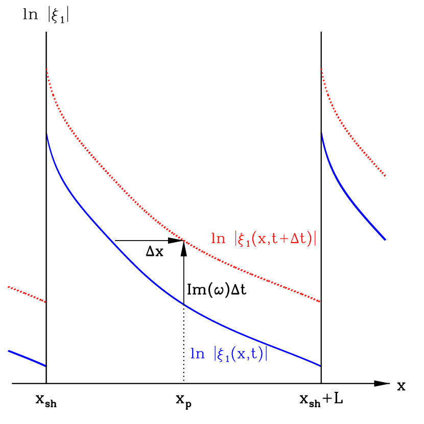
Figure 2.— Schematic profile of the perturbed PV for an unstable mode with ${\rm Im}(\omega)>0$ in between two consecutive shocks located at $x=x_{\rm sh}$ and $x_{\rm sh}+L$. The solid and dotted curves plot the amplitude of $\xi_{1}$ at time $t$ and $t+\Delta t$, respectively. The PV conservation requires that the increased PV at $x=x_{p}$ during the time interval $\Delta t$ should be equal to that advected from $x=x_{p}+\Delta x$, with $\Delta x=-u_{T0}\Delta t$.

Equation (34) states that the amplitude of PV is constant only for purely oscillatory modes with ${\rm Im}(\omega)=0$, whereas it keeps decreasing (increasing) with $x$ away from the shock for unstable (decaying) modes. Figure 2 exemplifies the situation with an unstable mode with ${\rm Im}(\omega)>0$, for which $\Xi_{1}$ grows in time. Since PV is preserved along a streamline, the increased PV at a certain position $x=x_{p}$ during the time interval $\Delta t$ due to instability should be equal to the advected PV from the upstream position separated by $\Delta x=-u_{T0}\Delta t$. This is possible when $\Xi_{1}$ is a decreasing function of $x$ for unstable modes.

In order for PV to be periodic in $x$, the spatial variation of $\Xi_{1}$ inevitably requires a sudden change of the PV amplitude at the shock front:

$$\left|\frac{\Xi_{1}^{s+}}{\Xi_{1}^{s-}}\right|=e^{2\pi{\rm Im}(\omega)/\Omega},$$ (39)

indicating that $|\Xi_{1}|$ should be enhanced (reduced) at the shock for unstable (decaying) modes. The PV conservation in between spiral shocks also requires that its phase should be different before and after the shock. Since the elapsed time between two successive shocks corresponds to $\tau=2\pi/\Omega$ and since $\int_{0}^{2\pi/\Omega}\mathcal{R}d\tau=\Sigma_{0}^{s+}L/(\Sigma_{c}u_{c})=2\pi\Sigma_{0}^{s+}/(\Sigma_{c}\Omega)$, equation (37) demands that $k_{x,v}/\Sigma_{0}$ should change at the shock as

$$\frac{k_{x,v}^{s-}}{\Sigma_{0}^{s-}}-\frac{k_{x,v}^{s+}}{\Sigma_{0}^{s+}}=\frac{q\Omega L}{u_{T0}\Sigma_{0}}k_{y}>0.$$ (40)

These changes in the amplitude and phase of the perturbed PV ought to be consistent with the shock jump conditions that we derive in the next subsection.

4.3. Shock Jump Conditions

4.3.1 Perturbed Shock Front

Perturbations of the form given in equation (26), applied to the background gas flow, also perturb the shock front into a sinusoidal shape. Define the shape of the perturbed shock front as

$$\zeta_{1}(x,y,t)=Z_{1}\exp(-i\omega t+ik_{y}y),$$ (41)

with amplitude $Z_{1}$. Then,

$$s\equiv x-x_{\rm sh}-\zeta_{1}$$ (42)

measures the displacement from the moving shock front, with $s=0$ corresponding to the instantaneous shock location (Lee & Shu, 2012).

The unit vector normal to the instantaneous shock front is given by

$$\hat{\bf n}=\frac{\nabla s}{|\nabla s|}\simeq(1,-ik_{y}\zeta_{1}),$$ (43)

to the first order in $\zeta_{1}$. On the other hand, the unit vector tangent to the shock front is

$$\hat{\bf t}=\left(\left.\frac{dx}{dy}\right|_{s},1\right)=(ik_{y}\zeta_{1},1),$$ (44)

(see Dwarkadas & Balbus 1996; Lee & Shu 2012). Thus, the velocity of the shock front is given as

$${\bf v}_{\rm sh}=\frac{\partial\zeta_{1}}{\partial t}\hat{\bf n}=(-i\omega\zeta_{1},0),$$ (45)

to the first order in $\zeta_{1}$.

The total gas surface density at the perturbed shock location can be written as

$$\Sigma(x_{\rm sh}+\zeta_{1})=\Sigma_{0}(x_{\rm sh})+\Sigma_{1}(x_{\rm sh})+\zeta_{1}\left.\frac{d\Sigma_{0}}{dx}\right|_{x_{\rm sh}},$$ (46)

where the last term denotes the Taylor expansion of $\Sigma_{0}$ to the perturbed shock position. The total gas velocity can similarly be expanded to yield expressions for $\mathbf{v}_{T}(x_{\rm sh}+\zeta_{1})$.

In the frame moving locally with the perturbed shock front, the perpendicular component of the total velocity relative to the shock front becomes

$$\begin{split}v_{\perp}=&\mathbf{v}_{T0}(x_{\rm sh}+\zeta_{1})\cdot\hat{\bf n}-{\bf v}_{\rm sh}\cdot\hat{\bf n}\\ =&u_{T0}+u_{1}+\zeta_{1}\frac{du_{T0}}{dx}+i\omega_{D}\zeta_{1},\end{split}$$ (47)

while the parallel component is

$$\begin{split}v_{\parallel}=&\mathbf{v}_{T0}(x_{\rm sh}+\zeta_{1})\cdot\hat{\bf t}-{\bf v}_{\rm sh}\cdot\hat{\bf t}\\ =&v_{T0}+v_{1}+\zeta_{1}\frac{dv_{T0}}{dx}+ik_{y}\zeta_{1}u_{T0}.\end{split}$$ (48)

Note that all quantities are evaluated at $x=x_{\rm sh}$ in equations (47) and (48).

4.3.2 Jump Conditions

Now we are ready to apply the Rankine-Hugoniot jump conditions across the shock fronts:

$$\Delta_{s}\left(v_{\perp}\Sigma\right) = 0,$$ (49a)

$$\Delta_{s}\left((c_{s}^{2}+v_{\perp}^{2})\Sigma\right) = 0,$$ (49b)

$$\Delta_{s}\left(v_{\parallel}\right) = 0,$$ (49c)

where $\Delta_{s}(f)$ again denotes the difference of $f$ between the immediate preshock and postshock regions.

Plugging equations (46), (47), and (48) into equations (49), one can show that the zeroth-order terms are identical to equations (20). Taking the first-order terms, equations (49) are simplified to

$$\Sigma_{0}u_{T0}\Delta_{s}\left(S_{1}\right)+\Delta_{s}\left(\Sigma_{0}U_{1}\right)+iZ_{1}\omega_{D}^{s}\Delta_{s}\left(\Sigma_{0}\right)=0,$$ (50a)

$$\left(\frac{u_{T0}^{2}+c_{s}^{2}}{2u_{T0}}\right)\Delta_{s}\left(S_{1}\right)+\Delta_{s}\left(U_{1}\right)+Z_{1}\Delta_{s}\left[\left(\frac{u_{T0}^{2}-c_{s}^{2}}{2u_{T0}^{2}}\right)\frac{du_{T0}}{dx}\right]=0,$$ (50b)

$$\Delta_{s}\left(V_{1}\right)-Z_{1}\left(\frac{\kappa^{2}}{2\Omega}\frac{u_{c}}{c_{s}^{2}}-ik_{y}\right)\Delta_{s}\left(u_{T0}\right)=0,$$ (50c)

where $\omega_{D}^{s}=\omega_{D}(x_{\rm sh})$.

4.4. Expansion near the Sonic Point

Equations (4.1) and (4.1) indicate that just like in the background steady spiral shocks, there are certain conditions that the perturbed quantities should obey at the sonic point to give regular solutions for the perturbation variables. To obtain these conditions, we expand $S_{1}$, $U_{1}$, and $V_{1}$ near $x=x_{\rm sp}$ as

$$S_{1} = A_{0}+A_{1}\delta\eta+\mathcal{O}(\delta\eta^{2}),$$ (51a)

$$U_{1}/(R\Omega) = B_{0}+B_{1}\delta\eta+\mathcal{O}(\delta\eta^{2}),$$ (51b)

$$V_{1}/(R\Omega) = C_{0}+C_{1}\delta\eta+\mathcal{O}(\delta\eta^{2}),$$ (51c)

with $A_{0,1}$, $B_{0,1}$, and $C_{0,1}$ being dimensionless constants.

Plugging equations (14) and (51) into equation (4.1), one can show that the zeroth-order and first-order terms in $\delta\eta$, respectively, yield

$$C_{0}=\frac{ia\tilde{\omega}_{D,\rm sp}A_{0}-(i\tilde{\omega}_{D,\rm sp}-2\alpha_{1})B_{0}}{(2+i\tilde{k}_{y}a)},$$ (52)

and

$$\begin{split}&a(2\alpha_{1}-i\tilde{\omega}_{D,\rm sp})A_{1}-(2\alpha_{1}-i\tilde{\omega}_{D,\rm sp})B_{1}\\ &=(i\tilde{\omega}_{D,\rm sp}\alpha_{1}-ia\tilde{k}_{y}\beta_{1m})A_{0}+(4\alpha_{2}+i\tilde{k}_{y}\beta_{1m})B_{0}\\ &-i\tilde{k}_{y}\alpha_{1}C_{0}-(2+i\tilde{k}_{y}a)C_{1},\end{split}$$ (53)

where $\tilde{\omega}_{D,\rm sp}=\omega/\Omega-(0.5-x_{\rm sp}/R+\beta_{0})\tilde{k}_{y}$, $\tilde{k}_{y}=Rk_{y}$, and $\beta_{1m}=\beta_{1}-1$. Equation (52) implies that $V_{1}$ at the sonic point cannot be taken arbitrarily: it should depend on $S_{1}$ and $U_{1}$ for transonic solutions to exist.

The zeroth-order terms of equation (4.1) are identical to equation (52). Its first-order terms give

$$\begin{split}&ia^{2}\tilde{\omega}_{D,\rm sp}A_{1}+a(4\alpha_{1}-i\tilde{\omega}_{D,\rm sp})B_{1}\\ &=i\tilde{k}_{y}a^{2}\beta_{1m}A_{0}+(i\tilde{\omega}_{D,\rm sp}\alpha_{1}-4a\alpha_{2}-i\tilde{k}_{y}a\beta_{1m})B_{0}\\ &+2\alpha_{1}C_{0}+a(i\tilde{k}_{y}a+2)C_{1}.\end{split}$$ (54)

On the other hand, the zeroth-order terms of equation (29) result in

$$C_{1}=-i\tilde{k}_{y}aA_{0}-\frac{u_{c}/(R\Omega)}{a^{2}}B_{0}+\frac{i\tilde{\omega}_{D,\rm sp}}{a}C_{0}.$$ (55)

Once $A_{0}$ and $B_{0}$ are known, therefore, $C_{0}$ and $C_{1}$ can be calculated from equations (52) and (55), respectively, and $A_{1}$ and $B_{1}$ by solving equations (53) and (54) simultaneously. This implies that the solutions near the sonic point are completely specified by two constants $A_{0}$ and $B_{0}$.

4.5. Method of Computation

Our problem involves four perturbation variables ($S_{1},U_{1},V_{1},Z_{1}$), one eigenvalue ($\omega$), three boundary conditions (eqs. [50a]–[50c]) and one constraint at the sonic point (eq. [52]). Since all the equations are linear, we may arbitrarily take the amplitude of one variable at the sonic point. Thus, the problem poses a well-defined eigenvalue problem, with four unknowns and four constraints.

In practice, we fix ${\rm Re}(A_{0})={\rm Im}(A_{0})=1$ at the sonic point, and choose two trial complex values for $\omega$ and $B_{0}$, which give the values of $S_{1}$, $U_{1}$, and $V_{1}$ as well as their derivatives at $x=x_{\rm sp}$. We integrate equations (4.1)–(29) from the sonic point both in the forward direction to $x=x_{\rm sh}+L$ and in the backward direction to $x=x_{\rm sh}$, and then apply the periodic conditions for the perturbation variables. At the shock front, equation (50c) gives $Z_{1}$, which can be used to check the first boundary condition (50a). If equation (50a) is not satisfied within a tolerance, we return to the first step and repeat the calculation by changing $B_{0}$. After equation (50a) is satisfied, we check the second boundary condition (50b). If equation (50b) is not fulfilled, we again return to the first step to change $\omega$, and continue the calculation iteratively until all the perturbed shock jump conditions are satisfied.

Table 2Eigenfrequencies of One-dimensional Perturbations

	$\mathcal{F}=0.03$			$\mathcal{F}=0.05$			$\mathcal{F}=0.1$
mode	${\rm Re}(\omega)/\Omega$	${\rm Im}(\omega)/\Omega$		${\rm Re}(\omega)/\Omega$	${\rm Im}(\omega)/\Omega$		${\rm Re}(\omega)/\Omega$	${\rm Im}(\omega)/\Omega$
1	$0.000$	$-2.657\times 10^{-1}$		0.000	$-3.727\times 10^{-1}$		0.354	$-6.363\times 10^{-1}$
2	$0.628$	$-9.230\times 10^{-2}$		0.692	$-1.782\times 10^{-1}$		0.809	$-3.897\times 10^{-1}$
3	$1.448$	$+4.438\times 10^{-4}$		1.496	$+1.222\times 10^{-3}$		1.614	$-1.078\times 10^{-2}$
4	$2.573$	$-6.212\times 10^{-3}$		2.628	$-1.380\times 10^{-2}$		2.740	$+7.693\times 10^{-3}$
5	$3.907$	$-5.982\times 10^{-3}$		4.023	$-2.758\times 10^{-2}$		4.316	$-3.565\times 10^{-2}$
6	$5.349$	$-1.120\times 10^{-2}$		5.554	$-2.543\times 10^{-2}$		6.019	$-5.747\times 10^{-2}$
7	$6.853$	$-1.560\times 10^{-2}$		7.144	$-2.618\times 10^{-2}$		7.846	$-5.831\times 10^{-2}$
8	$8.391$	$-1.935\times 10^{-2}$		8.759	$-3.077\times 10^{-2}$		9.663	$-8.771\times 10^{-2}$
9	$9.946$	$-1.537\times 10^{-2}$		10.389	$-2.555\times 10^{-2}$		11.509	$-7.421\times 10^{-2}$
10	$11.521$	$-1.941\times 10^{-2}$		12.033	$-2.250\times 10^{-2}$		13.352	$-8.511\times 10^{-2}$

5. Dispersion Relation

5.1. One-dimensional Modes

In this section, we apply the method described in Section 4 to the case of one-dimensional perturbations with $k_{y}=0$. We find there are a pure decaying mode (with ${\rm Re}(\omega)=0$ and ${\rm Im}(\omega)<0$) for small $\mathcal{F}$, a single overstable mode (with ${\rm Re}(\omega)\neq 0$ and ${\rm Im}(\omega)>0$), and many underdamping modes (with ${\rm Im}(\omega)<0$). Equations (4.1)–(29) and (50a)–(50c) guarantee that if $(S_{1},U_{1},V_{1})$ is a solution with eigenvalue $\omega$, then its complex conjugate is also a solution with eigenvalue $-\omega^{*}$, provided $k_{y}=0$. This indicates that eigenfrequencies exist always as a pair such that the imaginary parts are the same, while the real parts differ only in sign. We thus limit to the modes with ${\rm Re}(\omega)\geq 0$ in this subsection.

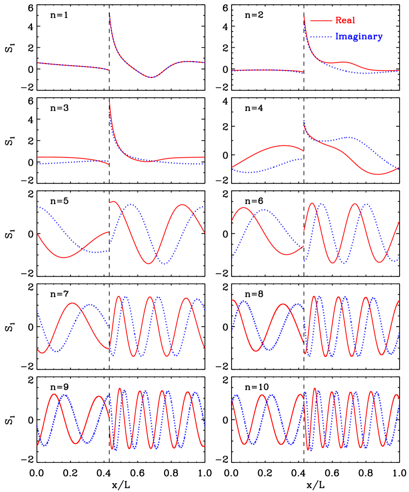
Figure 3.— Ten lowest-frequency eigenfunctions $S_{1}$ of axisymmetric modes with $k_{y}=0$ for $\mathcal{F}=5\%$. Solid and dotted lines correspond to the real and imaginary parts of $S_{1}$, respectively, normalized to unity at the sonic point located at $x/L=0.51$. They are identical to each other for a pure decaying, $n=1$ mode. The vertical line at $x/L=0.43$ in each panel marks the shock front.

In Table 2, we list ten lowest eigenfrequencies for $\mathcal{F}=3$, 5, and 10%. The modes are ordered in such a way that ${\rm Re}(\omega_{1})<{\rm Re}(\omega_{2})<{\rm Re}(\omega_{3})<\cdots$. Figure 3 plots the corresponding profiles of the perturbed density $S_{1}$ for $\mathcal{F}=5\%$, with the solid and dotted curves representing the real and imaginary parts, respectively. Note that ${\rm Re}(S_{1})={\rm Im}(S_{1})$ for the $n=1$ mode since ${\rm Re}(\omega)=0$. The vertical dashed line at $x/L=0.43$ marks the shock front. The number of nodes of the eigenfunctions is $2(n-3)$ for modes with $n\geq 5$. This indicates that the wavenumber $k_{x}$ in the $x$-direction increases with frequencies, which is a generic property of sound waves. We find that the real parts of the eigenfrequencies are well fitted by

$${\rm Re}(\omega)=(\langle u_{T0}\rangle+c_{s})k_{x},$$ (56)

with $k_{x}=2\pi(n-3)/L$ and the mean $x$-velocity $\langle u_{T0}\rangle/(L\Omega)=0.175,0.188$, and $0.216$ for $\mathcal{F}=3,5$, and $10\%$, respectively, which represents the “spatially-averaged” advection of sound waves by the background flow.

Sound waves propagating in a nonuniform medium naturally suffer amplification or decay depending on the sign of the density and velocity gradients relative to the propagation direction (e.g., Clarke & Carswell 2007). In addition, a shock wave not only reflects incident sound waves but also amplifies them upon transmission (e.g., Landau & Lifshitz 1987; Pijpers 1995). In the case of galactic spiral shocks, the eigenfrequencies given in Table 2 show that the non-uniform background and shock interactions usually dampen sound waves, with a decay rate larger for larger $\mathcal{F}$. Note that each spiral shock has a single mode with ${\rm Im}(\omega)>0$ ($n=3$ for $\mathcal{F}=3$ and $5\%$, and $n=4$ for $\mathcal{F}=10\%$). This indicates that steady, galactic spiral shocks are, in a strict sense, overstable to one-dimensional displacements along the direction perpendicular to the shock. The overstable mode grows faster when the shock is stronger and the background density varies more steeply. However, the growth time of the overstability is $t_{\rm grow}=2\pi/{\rm Im}(\omega)=8.2\times 10^{2}/\Omega$ even for $\mathcal{F}=10\%$, which is in general much longer than the Hubble time. This suggests that these one-dimensional equilibrium spiral shocks can be regarded stable for all practical purposes.

5.2. Two-dimensional Modes

We now search for two-dimensional normal modes with $k_{y}\neq 0$ and explore their stability. For the numerical examples below, we focus on the case with $\mathcal{F}=5\%$. The cases with different $\mathcal{F}$ are qualitatively similar.

5.2.1 Dispersion Relations

Unlike in the axisymmetric case, non-axisymmetric waves with $k_{y}\neq 0$ propagating in the positive and negative $y$-direction behave differently from each other due to the non-vanishing $v_{T0}$ in the background flow, making ${\rm Re}(\omega)$ depend on the sign of $k_{y}$. Figure 4 plots the dispersion relations of eight lowest-frequency eigenmodes over $|k_{y}L|\leq 30$ for $\mathcal{F}=5\%$. As in Figure 3, these modes are numbered in the increasing order of ${\rm Re}(\omega)$ at $k_{y}=0$. The dashed and solid lines show ${\rm Re}(\omega)$ and ${\rm Im}(\omega)$, respectively. It is apparent that ${\rm Re}(\omega)$ depends almost linearly on $k_{y}$, with a slope of $\sim(0.80-0.86)L\Omega$, indicating that the modes possess characteristics of acoustic waves or entropy-vortex waves or their linear combinations. Note that there are ranges of $k_{y}$ for which each mode becomes overstable. However, the corresponding growth rate remains smaller than $0.5\Omega$ except for the $n=7$ mode whose ${\rm Im}(\omega)$ keeps increasing with $k_{y}$.

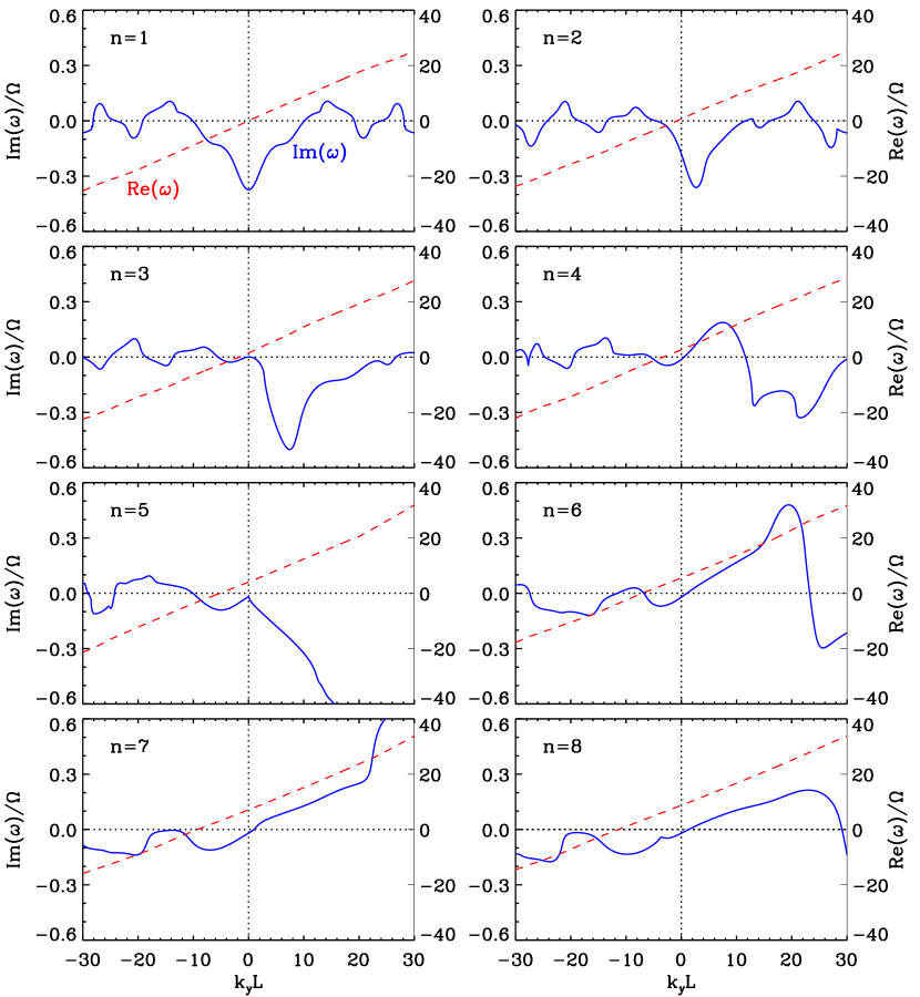
Figure 4.— Non-axisymmetric dispersion relations of the eight lowest-frequency eigenmodes for $\mathcal{F}=5\%$. The modes are numbered in the increasing order of ${\rm Re}(\omega)$ at $k_{y}=0$. In each panel, the blue solid line (left $y$-axis) gives ${\rm Im}(\omega)$, while the red dashed line (right $y$-axis) is for ${\rm Re}(\omega)$. The horizontal and vertical dotted lines mark $\omega=0$ and $k_{y}=0$, respectively.

Figure 5(a) plots an extended dispersion relation of the $n=7$ mode for $\mathcal{F}=5\%$, while Figure 5(b) compares the most unstable branches of the dispersion relations for differing $\mathcal{F}$: the $n=10$, 7, and 4 modes are plotted, respectively, for $\mathcal{F}=3$, 5, and 10%. By searching for all possible overstable modes, we have confirmed that these are the most unstable modes over $|k_{y}L|\leq 500$ for given $\mathcal{F}$. The growth rate and wavelength of the most unstable mode depend on $\mathcal{F}$ quite sensitively. The maximum growth rate ${\rm Im}(\omega)_{\rm max}/\Omega=0.32$, 1.36, and 4.71 occurs at $k_{y}L=32.2$, 92.4, and 204.5, with the corresponding real eigenfrequency of ${\rm Re}(\omega)/\Omega=38.1$, 100.6, and 198.3 for $\mathcal{F}=3$, 5, and 10%, respectively. Near the peak, ${\rm Im}(\omega)$ varies slowly with $k_{y}$. When $\mathcal{F}=5\%$, for example, modes with $k_{y}L\sim 85$–$105$ have growth rates within 1% of ${\rm Im}(\omega)_{\rm max}$. These modes of WI would grow very rapidly and are likely to readily manifest their presence in a galactic disk.

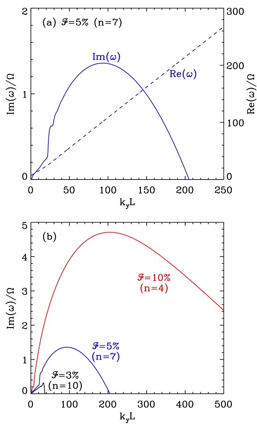
Figure 5.— (a) Extended non-axisymmetric dispersion relation of the $n=7$ mode for $\mathcal{F}=5\%$. The solid line (left $y$-axis) and the dashed line (right $y$-axis) draw ${\rm Im}(\omega)$ and ${\rm Re}(\omega)$, respectively. The maximum growth rate ${\rm Im}(\omega)_{\rm max}=1.36\Omega$ occurs at $k_{y}L=92.4$. (b) Dependence of ${\rm Im}(\omega)$ on $\mathcal{F}$. The $n=10$, 7, and 4 modes are plotted for $\mathcal{F}=3$, 5, and 10%, respectively.

The character of unstable or decaying modes can be identified by exploring their eigenfunctions. In the left panels of Figure 6, we plot the eigenfunctions $S_{1}$, $U_{1}$, $V_{1}$, and $\Xi_{1}$ of the most unable mode with $\omega/\Omega=100.6+1.36i$ for $\mathcal{F}=5\%$. The decaying counterparts with $\omega/\Omega=95.3-0.27i$ with the same $k_{y}$ and $\mathcal{F}$ are plotted in the right panels, for comparison. The vertical dashed line in each panel marks the shock front, while the dots in the top panels indicate the sonic point. For the unstable mode, it is clear that the amplitudes of the eigenfunctions decrease almost exponentially starting from the shock front toward the downstream direction, and experience large jumps at the shock, consistent with the prediction of equation (34). For the decaying mode, on the other hand, the amplitudes of the eigenfunctions except for $V_{1}$ increase with $x$ and exhibit sudden drops at the shock. For both cases, the $x$-wavenumber $k_{x}$ of the perturbations increase as they propagate away from the sonic point, making $k_{x}$ very large just before the shock, while it has relatively small values in the postshock regions. This spatial change of $k_{x}$ is due primarily to the shearing and expanding background flow.

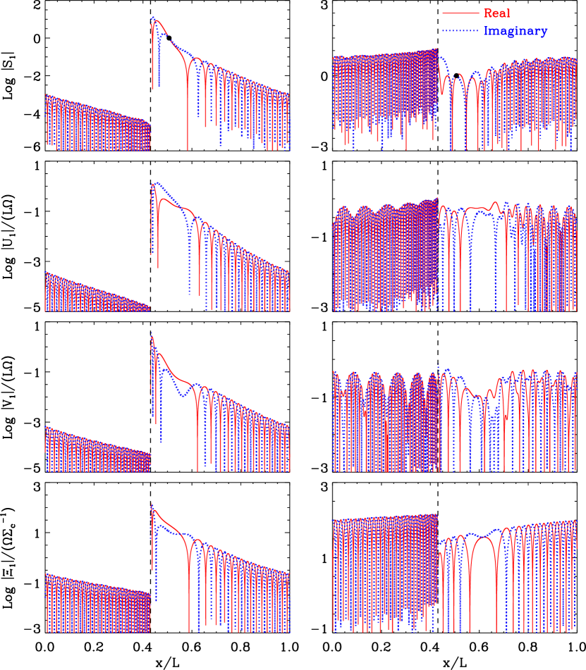
Figure 6.— Eigenfunctions of (left column) an unstable mode with $\omega/\Omega=100.6+1.36i$ and (right column) a decaying mode with $\omega/\Omega=95.3-0.27i$. For both modes, $\mathcal{F}=5\%$ and $k_{y}L=92.4$ are taken. The absolute values of the real and imaginary parts of $S_{1}$, $U_{1}$, $V_{1}$, and $\Xi_{1}$ are plotted as red solid and blue dotted curves, respectively. The vertical dashed line in each panel marks the shock front, while black dots in the top panels indicate the sonic point.

In general, any (linear) disturbance in the flow can be written as a superposition of an entropy-vortex wave and an acoustic wave (e.g., Landau & Lifshitz 1987):

$$\begin{split}S_{1}&=S_{1,v}+S_{1,a},\\ U_{1}&=U_{1,v}+U_{1,a},\\ V_{1}&=V_{1,v}+V_{1,a},\end{split}$$ (57)

where the quantities with the subscripts “$v$” and “$a$” stand for the contributions of the entropy-vortex and acoustic modes, respectively. These waves would decouple from each other in a uniform, non-rotating medium, but background gradients in the fluid quantities as well as galactic rotation in galactic shocks tend to mix them together unless their wavelengths are sufficiently small. The eigenfunctions shown in Figure 6 suggest that the WKB approximation (i.e., $k_{x}\gg|d\ln u_{T0}/dx|$) is valid only in the preshock regions. In this limit, one can show from equations (4.1)–(4.1) that the entropy-vortex modes with $x$-wavenumber $k_{x,v}$ are characterized by

$${\hat{\omega}_{v}}\equiv{\rm Re}(\omega)-u_{T0}k_{x,v}-v_{T0}k_{y}=0,$$ (58a)

$$S_{1,v}=2i\Omega/(c_{s}^{2}k_{y})U_{1,v},$$ (58b)

$$V_{1,v}=-(k_{x,v}/k_{y})U_{1,v},$$ (58c)

suggesting that these are incompressible and comoving with the background flow. Note that equation (58a) is identical to equation (36). For the acoustic modes, there are various ways to construct a WKB dispersion relation, but the acoustic parts of the decaying eigenfunctions presented in Figure 6 turn out to be best described by

$${\hat{\omega}_{a}}\equiv{\rm Re}(\omega)-u_{T0}k_{x,a}-v_{T0}k_{y}=-c_{s}k_{x,a},$$ (59a)

$$S_{1,a}=(k_{x,a}/\hat{\omega}_{a})U_{1,a}=-U_{1,a}/c_{s},$$ (59b)

$$V_{1,a}=(k_{y}/k_{x,a})U_{1,a},$$ (59c)

which is free of vorticity, with $k_{x,a}$ being the $x$-wavenumber of acoustic waves. For $k_{x}\gg k_{y}$, entropy-vortex modes have $|V_{1}|/|U_{1}|\gg 1$, while $c_{s}|S_{1}|\sim|U_{1}|\gg|V_{1}|$ for acoustic modes, showing that most of the wave energy is contained in $V_{1}$ for the former and in $S_{1}$ and $U_{1}$ for the latter.

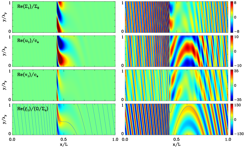
Figure 7.— Distributions on the $x$-$y$ plane of the real parts of the eigenfunctions of (left) the unstable mode and (right) the decaying mode shown in Figure 6, for Re$(\Sigma_{1})/\Sigma_{0}$, Re$(u_{1})/c_{s}$, Re$(v_{1})/c_{s}$, Re$(\xi_{1})/(\Omega\Sigma_{c}^{-1})$ from top to bottom at $t=0$. The ordinates are normalized by the wavelength $\lambda_{y}=2\pi/k_{y}=0.068L$. The wavefronts of the perturbed PV are overlaid as solid lines in the bottom panels.

Since $k_{x}$ becomes increasingly larger further downstream due to shear, the decomposition of waves using equations (57)–(59) is most meaningful in the regions just before the shock front. An inspection of the eigenfunctions shown in the left panels of Figure 6 reveals that $k_{x}^{s-}L=342.9$ and $V_{1}^{s-}/U_{1}^{s-}=-3.71$ in the immediate preshock regions, which are almost equal to the predictions of equations (58a) and (58c), demonstrating that the unstable modes are predominantly an entropy-vortex mode. On the other hand, the eigenfunctions of the decaying modes have $k_{x,a}^{s-}L=1535$ and $U_{1}^{s-}/S_{1}^{s-}=-0.97c_{s}$, roughly consistent with the predictions of equations (59a) and (59c), while $U_{1}^{s-}/V_{1}^{s-}\sim 3.2$ which cannot be described solely by either equation (58c) or equation (59c). This indicates that both acoustic and entropy-vortex modes contribute to the decaying mode, such that $S_{1}$ and $U_{1}$ are dominated by the acoustic mode with $k_{x,a}^{s-}/k_{y}=16.6$, while $V_{1}$ is affected by entropy-vortex modes. These results suggest that it is the entropy-vortex modes that become unstable to the WI, while the acoustic modes play a stabilizing role.

Using complex eigenfunctions, we can construct real perturbations as

$$\begin{split}{\rm Re}(\Sigma_{1})/\Sigma_{0}=e^{{\rm Im}(\omega)t}&\{{\rm Re}(S_{1})\cos[k_{y}y-{\rm Re}(\omega)t]\\ &-{\rm Im}(S_{1})\sin[k_{y}y-{\rm Re}(\omega)t]\},\end{split}$$ (60)

for the perturbed surface density, and similar expressions for the other perturbation variables. Figure 7 plots real eigenfunctions at $t=0$ on the $x$-$y$ plane of the (left column) unstable and (right column) decaying mode shown in Figure 6. Note that the $y$-axis is normalized by the perturbation wavelength $\lambda_{y}=2\pi/k_{y}$. The solid lines in the bottom panels represent constant phases of PV obtained by integrating equation (37) over $x$, which trace the wavefront of the perturbed PV very well. In the unstable case shown, the perturbed density and velocity are dominated by the entropy-vortex mode that is strongest in the postshock regions and becomes weaker in the downstream direction (see eq. [34]). At the immediate behind of the shock front, they have a trailing shape with $k_{x,v}>0$, progressively rotate into a less trailing shape due to shear reversal in the region with $\Sigma_{0}/\Sigma_{c}\geq 2$, and then become more trailing in the interarm regions. For the decaying modes, on the other hand, the wave amplitudes are stronger in the preshock regions, and the $x$-wavenumber of $\Sigma_{1}$ and $u_{1}$ dominated by acoustic waves is much larger than that of $v_{1}$ dominated by the entropy-vortex waves.

5.2.2 Physical Interpretation

Since PV is preserved along a streamline in between shocks, the fact that the WI relies on the entropy-vortex mode requires that vorticity should be generated at the shock discontinuities. In Appendix A, we utilize the shock jump conditions (50) to derive an expression for the PV changes at the shock. In the WKB limit, equation (A8) can be written as

$$\Xi_{1}^{s+}-\Xi_{1}^{s-}\approx\Delta_{U_{1}}+\Delta_{Z_{1}}+\Delta_{k_{x}},$$ (61)

where

$$\Delta_{U_{1}}\equiv ik_{y}\frac{(\mu-1)^{2}}{\mu^{2}}\frac{U_{1}^{s-}}{\Sigma_{0}^{s-}},$$ (62)

$$\Delta_{Z_{1}}\equiv-k_{y}\omega_{D}^{s}\frac{(\mu-1)^{2}}{\mu^{2}}\frac{Z_{1}}{\Sigma_{0}^{s-}},$$ (63)

and

$$\Delta_{k_{x}}\equiv-ik_{y}\frac{q\Omega L}{u_{T0}\Sigma_{0}}V_{1}^{s-}=i\Delta_{s}\left(\frac{k_{x,v}}{\Sigma_{0}}\right)V_{1}^{s-}.$$ (64)

Note that $\Delta_{U_{1}}$ originates from the tangential variation of the perpendicular velocity relative to the unperturbed shock, while $\Delta_{Z_{1}}$ results from the deformation of a shock front itself along the tangential direction. On the other hand, $\Delta_{k_{x}}$ is due to the discontinuity of $k_{x}/\Sigma_{0}$ across the shock (eq. [40]).

The role of the $\Delta$ terms in equation (61) in producing or reducing PV differs from each other. The first $\Delta_{U_{1}}$ term tends to decrease PV at the shock due to shock compression of the perpendicular velocity. To see this more clearly, for instance, let us consider a special case with $S_{1}=V_{1}=Z_{1}=0$, so that PV is contained in the $y$-variation of $U_{1}$. Then, equations (A6) and (A7) give $\Xi_{1}^{s+}/\Xi_{1}^{s-}=(2\mu-1)/\mu^{2}<1$ for any $\mu\geq 1$, showing that PV is reduced at the shock. Also, the third $\Delta_{k_{x}}$ term always tends to reduce PV across the shock, which can be seen as follows. Since entropy-vortex modes usually have $k_{x,v}/k_{y}>1$ due to shear, $\Xi_{1}^{s-}\approx i\omega_{D}^{sL}V_{1}^{s-}/(u_{T0}\Sigma_{0})$ from equation (A7) is a good approximation in the WKB limit. In this case, one can show that $\Delta_{k_{x}}/\Xi_{1}^{s-}\approx-(1+u_{T0}^{s-}k_{x,v}^{s-}/[q\Omega Lk_{y}])^{-1}<0$. Physically, this arises since the background shearing flow has $k_{x,v}^{s+}/k_{x,v}^{s-}<\mu$ (e.g., equation [40]), which in turn makes $\Xi_{1}\sim k_{x}V_{1}/\Sigma_{0}$ decreased after the shock jump.

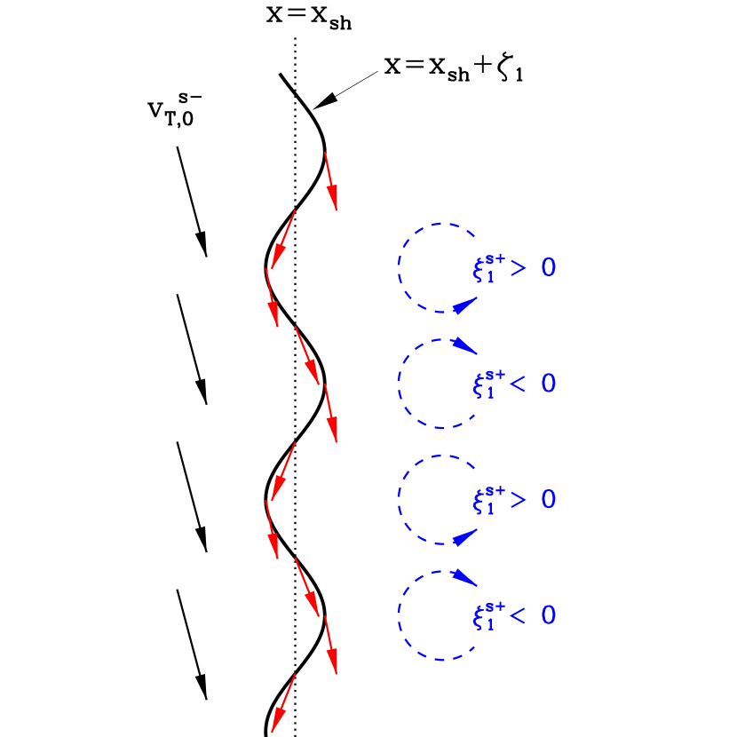
Figure 8.— Schematic diagram showing the production of PV at the distorted shock front ($x=x_{\rm sh}+\zeta_{1}$). The vertical dotted line indicates the unperturbed shock location ($x=x_{\rm sh}$). The black arrows on the left represent the background flow velocity $\mathbf{v}_{T0}^{s-}$ seen in the frame comoving with the deformed shock front. The red arrows indicate the directions of the flow immediate after the shock. The resulting PV is positive at the $y$-positions where $\zeta_{1}<0$ and negative where $\zeta_{1}>0$, as indicated by the dashed arrows.

On the other hand, the $\Delta_{Z_{1}}$ term is a source for the PV production at a deformed shock front, as Crocco’s theorem suggests. Figure 8 schematically illustrates the PV generation and the relationship between the signs of $\xi_{1}$ and $\zeta_{1}$. The vertical dotted line and thick sinusoidal curve indicate the unperturbed and perturbed shock fronts, respectively. Since ${\rm Re}(\omega)/k_{y}>v_{T0}(x_{\rm sh})$ (or $\omega_{D}^{s}>0$) from the linear dispersion relation, the deformed shock front moves faster along the $y$-direction than the background flow at the shock. Viewed in the stationary shock frame, therefore, the background gas is moving in the negative $y$-direction, as represented by the black arrows on the left. In traversing the shock, the velocity vectors bend toward the local tangent to an instantaneous shock front, which are indicated by the red arrows. This naturally produces nonvanishing PV (marked by dashed curved with arrows) in the postshock flow. The sign of the PV depends on the shape of the shock front, such that it is positive (negative) in the regions where the shock is convex (concave) seen from the upstream direction. That is, $\xi_{1}$ and $\zeta_{1}$ have opposite signs, consistent with equation (63).

When the $\Delta_{Z_{1}}$ terms dominates the other terms, PV contained in the entropy-vortex waves can grow whenever the waves pass through distorted spiral shocks in the course of galaxy rotation. Interactions of traveling waves in the $x$-direction form a standing entropy-vortex mode that can grow exponentially in time, leading to the WI. That is, the WI refers to the growth of entropy-vortex modes owing to vorticity generation from distorted spiral shocks that the interstellar gas in galaxy rotation meets periodically. On the other hand, either when $U_{1}$ dominates the perturbations, a most likely situation where acoustic modes are stronger than entropy-vortex modes, or when $V_{1}$ dominates (without involving strong shock deformations), PV drops at the shocks and the associated entropy-vortex mode becomes weaker with time. This PV reduction is responsible for the decaying modes shown in Figures 4 and 6. Since $\Delta_{k_{x}}/\Delta_{Z_{1}}\propto k_{y}L/\omega_{D}^{s}$, the $\Delta_{k_{x}}$ term becomes predominant for very large $k_{y}$, eventually stabilizing the WI at $k_{y}L\lower 2.15277pt\hbox{$\;\buildrel>\over{\sim}\;$}205$ for the dispersion relation displayed in Figure 5(a).

6. Numerical Simulation

To check the wavelength and growth rate of the most unstable mode of the WI found in the preceding section, we run direct numerical simulations using the Athena code (Stone et al., 2008; Stone & Gardiner, 2009). Athena is an Eulerian code for compressible magnetohydrodynamics based on high-order Godunov schemes. In this work, we use the constrained corner transport method for directionally unsplit integration, the HLLC Riemann solver for flux computation, and the piecewise linear method for spatial reconstruction.

We first apply the Athena code to set up one-dimensional equilibrium shock profiles for $\mathcal{F}=5\%$. The other galaxy and arm parameters are taken the same as in the normal-mode analysis. The simulation domain has a length of $L$, which is resolved by 2048 zones. In order to avoid strong non-steady gas motions induced by a sudden introduction of the spiral potential, we increase its amplitude slowly to make it achieve the full strength at $t\Omega=50$. The system reaches a quasi-steady state at $t\Omega=100$, where the density distribution consists of a steady part and a small-amplitude fluctuating part. We have confirmed that the steady part is almost identical to that shown in Figure 1.

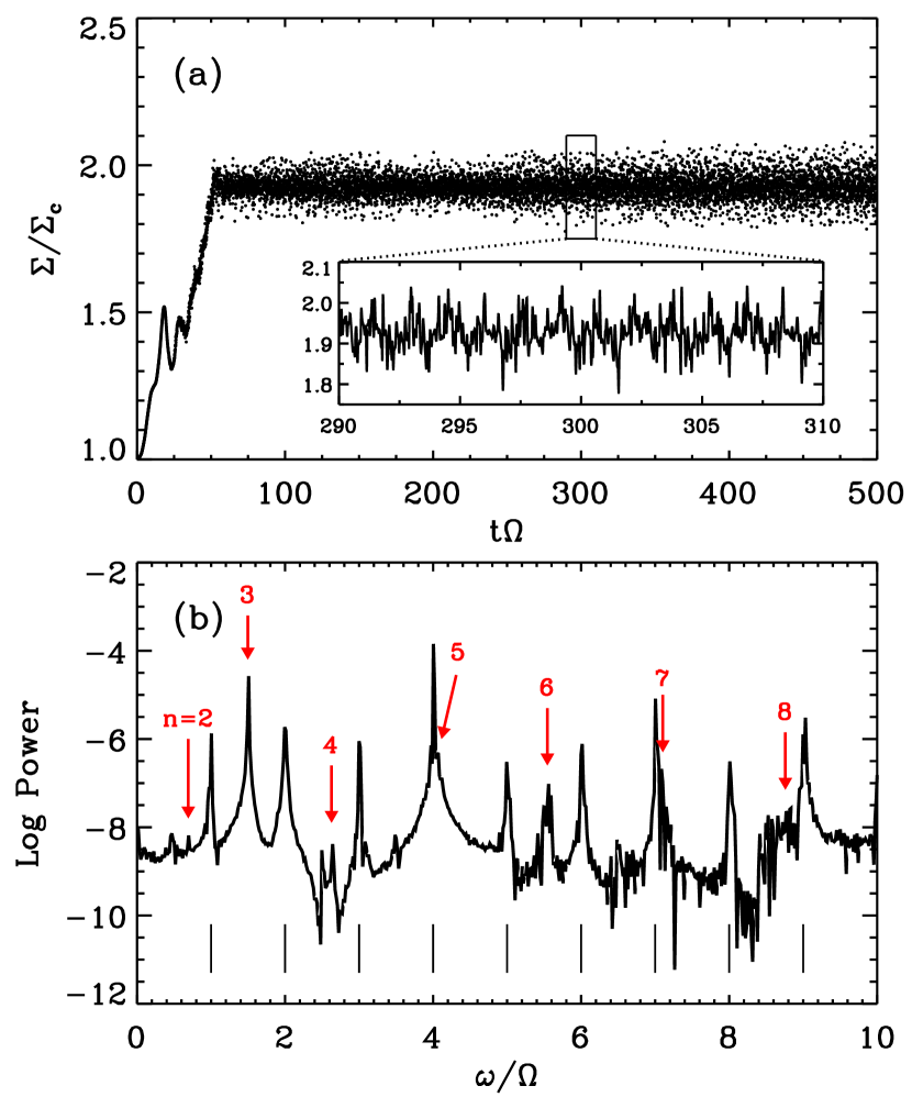
Figure 9.— (a) Temporal variation of the gas surface density at $x/L=0.5$ from a one-dimensional simulation with $\mathcal{F}=5\%$, and (b) its power spectrum. The inset in (a) zooms in the time range $290\leq t\Omega\leq 310$ to clearly show fluctuations of $\Sigma$. The presence of various modes makes $\Sigma$ fluctuate with time, with its amplitude growing very slowly due to an overstable ($n=3$) mode. The frequencies marked by short solid lines in (b) correspond to the orbital crossing time and its higher harmonics, while those indicated by red arrows represent the real parts of the eigenvalues given in Table 1.

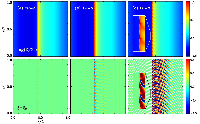
Figure 10.— Snapshots of (upper panels) gas surface density and (lower panels) perturbed PV at $t/\Omega=3$, 5, and 8 from a two-dimensional run with $\mathcal{F}=5\%$ and $2048\times 2048$ resolution. The wavefronts of the PV obtained by integrating equation (37) are overlaid in the bottom right panel. The number of the most unstable mode along the $y$-direction is 16 over the distance of $L$. The insets in (c) enlarge the section at $0.405\leq x/L\leq 0.455$ and $0.30\leq y/L\leq 0.45$. The upper and lower colorbars label $\log(\Sigma/\Sigma_{c})$ and $\xi-\xi_{0}$ in units of $\Omega\Sigma_{c}^{-1}$, respectively.

To examine the frequencies of the fluctuating density field, we monitor the temporal evolution of the gas surface density at $x/L=0.5$, which is plotted in Figure 9 together with its Fourier-transformed power spectrum over $t\Omega=200-500$. The mean and standard deviation of $\Sigma/\Sigma_{c}$ is $\sim 1.926$ and $0.040$, respectively. Note that the power spectrum is peaked at some specific frequencies. The frequencies marked by the short line segments at the bottom of Figure 9(b) are the integral multiples of $\Omega$, corresponding to the gas crossing time across the simulation box and its higher harmonics. On the other hand, the frequencies indicated by the arrows with numbers are very close to those given in Table 2, indicating that these represent decaying or growing eigenmodes identified in the normal-mode analysis. We note that among such modes, the $n=3$ mode with ${\rm Re}(\omega)/\Omega=1.496$ has largest power since it is an overstable mode. Figure 9(a) indeed shows a growing trend of the gas surface density due to overstability, although the amplification factor is only 60% over $\Delta t\Omega=400$ because of too low a growth rate.

Next, we simulate the WI of a spiral shock on the $x$-$y$ plane. We take the one-dimensional shock profile with $\mathcal{F}=5\%$ as a background state. We initially apply small-amplitude density perturbations that are realized by a Gaussian random field with flat power, with a standard deviation of $10^{-3}\Sigma_{0}$. For the simulation domain, we set up a square box with size $L\times L$ and implement the shearing box boundary conditions that can naturally handle shear in the background flow (Hawley et al., 1995; Kim & Ostriker, 2002, 2006). We set up a uniform Cartesian grid with various resolutions. Since the WI grows at scales much smaller than $L$, it is necessary to run high-resolution simulations to resolve it properly. We find that models with $1024\times 1024$ zones or higher give converged results, while those with $512\times 512$ zones or less overestimate the wavelength of the most unstable mode $\lambda_{y,\rm max}$. This suggests that $\lambda_{y,\rm max}$ should be resolved by no smaller than 64 zones in order to accurately capture the WI.

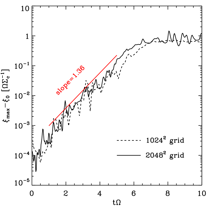
Figure 11.— Evolution of the maximum PV measured at $x/L=0.45$ for the $\mathcal{F}=5\%$ models with $1024\times 1024$ and $2048\times 2048$ zones. The growth rates measured from the simulations are consistent with the results of the normal-mode linear stability analysis, marked by the line segment with slope of $1.36$. The WI saturates nonlinearly at $t\Omega\lower 2.15277pt\hbox{$\;\buildrel>\over{\sim}\;$}7$.

Figure 10 displays snapshots of (upper panels) density structures in logarithmic scale and (lower panels) PV distributions in linear scale at $t\Omega=3$, 5, and 8, from a run with $2048\times 2048$ resolution. Figure 11 compares the time histories of the maximum PV relative to the initial value, $\xi_{\rm max}-\xi_{0}$, measured at $x/L=0.45$ from models with $1024\times 1024$ and $2048\times 2048$ zones. Initially, various waves seeded by the density perturbations interact with the background flow, and try to find eigenmodes that grow or decay depending on the sign of ${\rm Im}(\omega)$. The system soon picks up a few modes that have large ${\rm Im}(\omega)$ and non-negligible initial power. At $t\Omega=3$, the amplitudes of these modes are too small to be readily discernible in the snapshots. They keep growing during the linear phase that lasts until $t\Omega\sim 7$, after which the growth of the WI saturates. Figure 10 shows that the wavenumber of the most strongly growing mode at $t\Omega\lower 2.15277pt\hbox{$\;\buildrel>\over{\sim}\;$}5$ is $k_{y}L\sim 32\pi=100.5$, which is close to $k_{y,\rm max}L=92.4$ predicted from the linear stability analysis. The dominance of the $k_{y}L\sim 100.5$ mode in the simulations is caused by a combination of two facts: (1) its growth rate is only 0.5% smaller than, and is thus almost indistinguishable from that of the most unstable mode (see Figure 5), and (2) it has an initial amplitude about an order of magnitude larger than the latter in our density perturbations.

The insets of Figure 10(c) zoom in the section at $0.405\leq x/L\leq 0.455$ and $0.30\leq y/L\leq 0.45$ to clearly display the distortion of the shock front. Note that $\xi-\xi_{0}$ is positive (negative) in the regions where the shock is displaced toward the upstream (downstream) direction, consistent with Figure 8. Consistent also with the shape of the eigenfunctions, the density and PV distributions of the WI in the numerical simulations have the shapes that are trailing as the gas leaves the spiral shock, become less trailing in the region of shear reversal $(0.43\leq x/L\leq 0.50)$, and then become more trailing afterwards. The growth rate of this mode measured from the simulations is consistent with the prediction of the linear stability analysis, plotted as a line segment with slope of $1.36$ in Figure 11. The white lines overlaid in the bottom-right panel of Figure 10 are the wavefronts obtained by integrating equation (37), which are in good agreement with the PV distributions in our simulations. All of these validate the results of both our normal-mode stability analysis and numerical simulations.

7. Summary and Discussion

We have presented the results of a normal-mode linear stability analysis and hydrodynamic simulations for the WI of galactic spiral shocks by employing a local shearing-box model of a galactic gaseous disk under flat rotation. We assume that the disk is infinitesimally thin and remains isothermal, and do not consider the effects of magnetic fields and gaseous self-gravity, for simplicity. We first obtain one-dimensional profiles of time-independent spiral shocks (Section 3). We then apply small-amplitude perturbations to the steady solutions, and derive the differential equations and the shock jump conditions that the perturbation variables obey (Section 4). By solving the perturbation equations as eigenvalue and boundary-value problems, we obtain dispersion relations for various overstable and decaying modes (Section 5). We also compare the results of the linear stability analysis with those of numerical simulations (Section 6).

The dispersion relations show that there are various ranges of $k_{y}$ with which entropy-vortex modes become overstable, proving that the WI is physical, rather than numerical, in origin. While PV remains constant in a Lagrangian sense in between shocks, we show that it experiences a sudden change across a shock primarily by the following three processes: (1) tangential deformation of a shock front, (2) tangential variation of the perturbed velocity perpendicular to the unperturbed shock, and (3) discontinuity of $k_{x}/\Sigma_{0}$ across the shock. The first one increases the PV at the shock, as a consequence of Crocco’s theorem. On the other hand, the last two processes tend to decrease PV through shock compression and shear reversal across the shock, respectively. When the first process dominates, PV of a gas element keeps increasing whenever it passes through spiral shocks on its way of galaxy rotation. The continuous increase of PV in a Lagrangian sense is realized in our Eulerian stability analysis by standing entropy-vortex modes that grow exponentially with time, leading to the WI. Sound waves and the jumps in $k_{x}/\Sigma_{0}$ tend to suppress the WI, with the stabilizing effect of the latter predominating for very short wavelength perturbations. For $\mathcal{F}=5\%$, the most unstable modes are found to have a growth rate comparable to the orbital angular frequency $\Omega$ occurring at $k_{y}L\sim 10^{2}$, although these become larger for higher $\mathcal{F}$. We confirm that the growth rate and wavelength of the most unstable mode found in the linear stability analysis are consistent with the results of direct numerical simulations.

The assertion of Wada & Koda (2004) that the WI was due to the KHI was based on their result that a shear layer behind the shock has the Richardson number $J<1/4$. As they noted, however, $J>1/4$ is only a necessary condition for stability (Chandrasekhar, 1961), so that $J<1/4$ should not be interpreted as an instability criterion for KHI. On the other hand, we have shown in the present work that the WI relies on the vorticity generation from a deformed shock front. Although both WI and KHI involve vorticity, they differ in several remarkable ways. First, the PV generation in the WI necessitates the presence of a shock, which in turn requires non-vanishing perpendicular velocity $u_{T0}$ and density compression factor $\mu>1$, while the KHI occurs when $u_{T0}=0$ and $\mu=1$. Second, the WI is global in the sense that it requires successive passages of a gas flow across spiral shocks, which is attained by the periodic boundary conditions in the current Eulerian analysis. On the other hand, the KHI, when interpreted in terms of vorticity dynamics, occurs as vorticity produced by disturbing an interface between two fluids moving in opposite directions is accumulated at points where it amplifies the interface distortion (e.g., Batchelor 1967; Drazin 2002), indicating that it is local. Third, the WI is stabilized at very large $k_{y}$ by shear reversal across the shock front, while the KHI grows faster at larger $k_{y}$ (in the absence stabilizing agents such as viscosity, conduction, etc., that are not considered in this work). These differences clearly indicate that the WI studied in this work cannot be attributed to KHI. Referring to the work of Wada & Koda (2004), Renaud et al. (2013) mentioned KHI as a clump formation mechanism in their high-resolution simulations. But, the locations (postshock regions) and overall shapes (trailing as they leave the shocks) as well as spacing ($\sim 0.2{\rm\,kpc}$) of clumps shown in their Figure 13 are similar to those of the eigenfunctions and wavelength of the WI (e.g., Figs. 7 and 10), suggesting that they are the products of the WI rather than the KHI.

Dobbs & Bonnell (2006) presented the results of SPH simulations for cloud formation in spiral galaxies without considering the effects of magnetic fields and self-gravity (see also Dobbs et al. 2006). They showed that spiral shocks efficiently form gas clumps that are sheared out in the interarm regions to appear as feathers only if gas is cold, while warm gas with $T>10^{4}$ K is unable to produce clumps. They interpreted the clump formation in their cold-gas model as being arising from angular momentum exchanges among particles in the shock that are already inhomogeneous before entering the shock. Similarities between their density maps and those in Wada & Koda (2004) strongly suggest that the clump formation in their SPH models is most likely due to the WI. In the picture of WI, colder gas is more prone to the instability since it induces stronger shocks, corresponding to larger $\mathcal{F}$.

In this work we take an eigenvalue approach to analyze the stability of spiral shocks. Dwarkadas & Balbus (1996) took another approach by solving a linearized set of hydrodynamic equations as an initial value problem subject to the shock jump conditions. Since the two methods are complementary to one another, they should yield the same results. However, Dwarkadas & Balbus (1996) reported that non-self-gravitating and unmagnetized shocks are linearly stable due possibly to the non-vanishing radial velocity, which is seemingly in contrast to our results. We note that their conclusion was based on long-wavelength perturbations with $k_{y}L\sim 1$, about two orders of magnitude smaller than $k_{y,\rm max}$ found in the present work, which were evolved only up to $t\Omega\sim 1$. Figure 4 shows that modes with $|k_{y}|L\leq 1$ can also be unstable, although their growth rates are less than $\sim 0.015\Omega^{-1}$. Since the corresponding amplification factor over one orbital period is less than 10%, they were unlikely to grow to appreciable amplitudes in the work of Dwarkadas & Balbus (1996). In addition, such slowly growing modes could easily be suppressed by numerical viscosity present in any numerical scheme (e.g., Kim et al. 2010; Kim & Stone 2012).

While we have shown that the WI grows very rapidly in a razor-thin disk with no magnetic field, it still remains to be seen whether it is responsible for dense arm clouds and feathers in real spiral galaxies for the following two reasons. First, it is unclear whether the WI would operate in disks that are magnetized and vertically stratified. Kim & Ostriker (2006) showed that spiral shocks exhibit flapping motions in the direction perpendicular to the arm, when the vertical degree of freedom is considered. These motions are caused by incommensurability between the arm-to-arm crossing time with the vertical oscillation periods, capable of injecting turbulent energy into dense post-shock gas (Kim et al., 2006, 2008). These non-steady motions as well as strong vertical shear present in three-dimensional shocks appear to disrupt coherence of vortical structures at different heights, preventing the growth of WI (Kim & Ostriker, 2006). In addition, the presence of magnetic fields appears to stabilize WI (Dobbs & Price, 2008) and completely quenches it when the fields are of equipartition strength or stronger (Shetty & Ostriker, 2006), although it is uncertain whether the magnetic stabilization is due to magnetic forces on the perturbations or through a reduced background shock strength.

Second, even if the WI does develop in real disk galaxies, the connection between the WI and observed giant clouds and interarm feathers is not direct. The WI itself involves perturbations only near the shock front, resulting in very weak perturbations in the interarm regions. It also occurs at very small spatial scales, corresponding to 0.07 times the arm-to-arm spacing when $\mathcal{F}=5\%$ and even smaller scales when the arms are stronger. On the other hand, observed feathers and giant clouds in the arms of M51 have a mean separation of order $\sim(0.5-2)$ kpc (e.g., Elmegreen & Elmegreen 1983; Schinnerer et al. 2013), consistent with the Jeans length at the arm density peak (e.g., Elmegreen 1994; Kim & Ostriker 2002), and appear quite strong also in the interarm regions. Recently, Lee & Shu (2012) carried out a linear stability analysis of feathering instability by including self-gravity and magnetic fields. They showed that feathering modes retain relatively strong presence in the interarm regions and grow sufficiently rapidly, indicating that self-gravity may be essential for the formation of interarm feathers. All of these suggest that the WI alone is unlikely responsible for interarm feathers. Of course, it cannot be ruled out the possibility that small clumps produced primarily by the WI become denser by self-gravity, radiative cooling, and/or through mutual mergers, as in high-density clumps produced in models of Renaud et al. (2013), possibly developing into feathers in the downstream side. It would thus be interesting to explore the effects of self-gravity and magnetic fields on the WI, and their relationships with nonaxisymmetric interarm features.

Appendix A Jump of Potential Vorticity at the Perturbed Shock Front

Galactic gas flows periodically meet spiral shocks, once in every $2\pi/\Omega$ interval. While PV is conserved along a given streamline in between shocks, it inevitably experiences a sudden jump when moving across a distorted shock. In this Appendix, we derive the jump condition for the perturbed PV, $\Delta_{s}\left(\Xi_{1}\right)=\Xi_{1}^{s+}-\Xi_{1}^{s-}$, at the shock front ($x=x_{\rm sh}$).

We first want to express $S_{1}^{s+}$, $U_{1}^{s+}$, and $V_{1}^{s+}$ in terms of $S_{1}^{s-}$, $U_{1}^{s-}$, $V_{1}^{s-}$, and $Z_{1}$. It is useful to write

$$u_{T0}^{s+}=c_{s}\mu^{-1/2},\;\;\;\text{and}\;\;\;u_{T0}^{s-}=c_{s}\mu^{1/2},$$ (A1)

from equations (21) and (22). It then follows that

$$\frac{d}{dx}\ln(u_{T0}^{s+}u_{T0}^{s-})=-(\mu-1)\frac{d\ln u_{T0}^{s-}}{dx},$$ (A2)

from equation (11).

With the help of equations (A1) and (A2), we solve equations (50a) and (50b) for $S_{1}^{s+}$ and $U_{1}^{s+}$ to obtain

$$S_{1}^{s+}=S_{1}^{s-}+\frac{2}{c_{s}\mu^{1/2}}\left(U_{1}^{s-}+i\omega_{D}^{s}Z_{1}-\frac{\mu-1}{2}\frac{du_{T0}^{s-}}{dx}Z_{1}\right),$$ (A3)

$$U_{1}^{s+}=-\frac{1}{\mu}U_{1}^{s-}-i\omega_{D}^{s}\left(1+\frac{1}{\mu}\right)Z_{1}+\frac{\mu-1}{\mu}\frac{du_{T0}^{s-}}{dx}Z_{1},$$ (A4)

for $\mu\neq 1$. Here, $\omega_{D}^{s}=\omega_{D}(x_{\rm sh})$. Equation (50c) simply results in

$$V_{1}^{s+}=V_{1}^{s-}-\frac{\mu-1}{\mu^{1/2}}\left(\frac{\kappa^{2}}{2\Omega}\frac{u_{c}}{c_{s}}-ik_{y}c_{s}\right)Z_{1}.$$ (A5)

These are the jump conditions that the perturbation variables should satisfy at the shock front.

Substituting equation (29) in equation (33) and arranging the terms using equations (A3)–(A5), we obtain the perturbed PV immediate behind of the shock

$$\begin{split}\Xi_{1}^{s+}=&\left(ik_{y}\frac{1-2\mu}{\mu^{2}}-\frac{\kappa^{2}}{2\Omega}\frac{u_{c}}{\mu c_{s}^{2}}\right)\frac{U_{1}^{s-}}{\Sigma_{0}^{s-}}-\left(ik_{y}\frac{c_{s}^{2}}{u_{T0}^{s-}}+\frac{\kappa^{2}}{2\Omega}\frac{u_{c}}{u_{T0}^{s-}}\right)\frac{S_{1}^{s-}}{\Sigma_{0}^{s-}}\\ &+\frac{i\omega_{D}^{s}}{u_{T0}^{s-}}\frac{V_{1}^{s-}}{\Sigma_{0}^{s-}}-k_{y}\omega_{D}^{s}\frac{(\mu-1)^{2}}{\mu^{2}}\frac{Z_{1}}{\Sigma_{0}^{s-}}+ik_{y}\frac{(\mu-1)^{2}}{\mu^{2}}\frac{du_{T0}^{s-}}{dx}\frac{Z_{1}}{\Sigma_{0}^{s-}},\end{split}$$ (A6)

while the perturbed PV ahead of the shock is given by

$$\begin{split}\Xi_{1}^{s-}=&-\left(ik_{y}+\frac{\kappa^{2}}{2\Omega}\frac{u_{c}}{\mu c_{s}^{2}}\right)\frac{U_{1}^{s-}}{\Sigma_{0}^{s-}}-\left(ik_{y}\frac{c_{s}^{2}}{u_{T0}^{s-}}+\frac{\kappa^{2}}{2\Omega}\frac{u_{c}}{u_{T0}^{s-}}\right)\frac{S_{1}^{s-}}{\Sigma_{0}^{s-}}+\frac{i\omega_{D}^{sL}}{u_{T0}^{s-}}\frac{V_{1}^{s-}}{\Sigma_{0}^{s-}},\end{split}$$ (A7)

where $\omega_{D}^{sL}=\omega_{D}(x_{\rm sh}+L)=\omega_{D}^{s}+q\Omega Lk_{y}$.

Subtraction of equation (A7) from equation (A6) gives the jump condition for the PV across the perturbed shock

$$\Delta_{s}\left(\Xi_{1}\right)=ik_{y}\frac{(\mu-1)^{2}}{\mu^{2}}\frac{1}{\Sigma_{0}^{s-}}\left(U_{1}^{s-}+\frac{du_{T0}^{s-}}{dx}Z_{1}+i\omega_{D}^{s}Z_{1}\right)-ik_{y}\frac{q\Omega L}{u_{T0}\Sigma_{0}}V_{1}^{s-},$$ (A8)

which can be rewritten in a more illuminating form as

$$\Delta_{s}\left(\xi_{1}\right)=\frac{(\mu-1)^{2}}{\mu^{2}}\frac{1}{\Sigma_{0}^{s-}}\frac{\partial v_{\perp,1}^{s-}}{\partial y}-\frac{q\Omega L}{u_{T0}\Sigma_{0}}\frac{\partial v_{1}^{s-}}{\partial x},$$ (A9)

with

$$v_{\perp,1}^{s-}=u_{1}^{s-}+\zeta_{1}(du_{T0}^{s-}/dx)+i\omega_{D}^{s}\zeta_{1},$$ (A10)

being the perturbed preshock velocity perpendicular to the instantaneous shock front (see eq. [47]). The second term in the right-hand side of equation (A9) follows from equations (33) and (40), resulting originally from non-uniform background shear across a shock front. Equation (A9) states that the PV jump at the shock is due to two factors : the tangential variation of the perpendicular velocity and the discontinuous change of $k_{x,v}/\Sigma_{0}$ at the shock.

The origin of the first term in equation (A9) is Crocco’s theorem for vorticity generation from a curved shock front. Hayes (1957) showed that the vorticity jump across an unsteady shock amounts to

$$\Delta_{s}\left(\nabla\times\mathbf{v}|_{z}\right)=-\frac{(\mu-1)^{2}}{\mu}\left(V_{s}K+\frac{\partial C_{r}}{\partial S}\right),$$ (A11)

where $K$ is the curvature of the shock front, $V_{s}$ is the tangential component of the fluid velocity, $C_{r}$ is the shock speed relative to the normal component of the preshock fluid velocity, and $S$ denotes the coordinate tangential to the shock (see also Truesdell 1952; Kevlahan 1997). Noting that spiral shocks in our local models are straight $(K=0)$, one can see that $\Delta_{s}\left(\Xi_{1}\right)=\Delta_{s}\left(\nabla\times\mathbf{v}|_{z}\right)/\Sigma_{0}^{s-}$ with $C_{r}=-v_{\perp,1}^{s-}$ and $S=y$ in the absence of background shear ($q\Omega=0$).

References

- Baade (1963) Baade, W. 1963, in The Evolution of Stars and Galaxies, ed. C. Payne-Gaposchkin (Cambridge: Harvard Univ. Press), 218
- Balbus (1988) Balbus, S. A. 1988, ApJ, 324, 60
- Balbus & Cowie (1985) Balbus, S. A., & Cowie, L. L. 1985, ApJ, 297, 61
- Balmforth & Korycansky (2001) Balmforth, N. J., & Korycansky, D. G. 2001, MNRAS, 326, 833
- Batchelor (1967) Batchelor, G. K. 1967, An Introduction to Fluid Dynamics (Cambridge Univ. Press), pp. 511-516
- Bates (2007) Bates, J. W. 2007, PhFl, 19, 094102
- Buta (2013) Buta R. 2013, Secular Evolution of Galaxies: XXIII Canary Islands Winter School of Astrophysics, eds. J. Falcon-Barroso, & J. Knapen (Cambridge: Cambridge University Press), p.155
- Buta & Combes (1996) Buta R., & Combes F. 1996, Fund. Cosmic Phys., 17, 95
- Chandrasekhar (1961) Chandrasekhar, S. 1961, Hydrodynamic and Hydromagnetic Stability (Dover: New York), 491
- Clarke & Carswell (2007) Clarke, C. J., & Carswell, R. F. 2007, Principles of Astrophysical Fluid Dynamics (New York: Cambridge University Press)
- Corder et al. (2008) Corder, S., Sheth, K., Scoville, N. Z., et al. 2008, ApJ, 689, 148
- de Val-Borro et al. (2007) de Val-Borro, M., Artymowicz, P, D’Angelo, G., & Peplinski, A. 2007, A&A, 471, 1043
- Dobbs & Bonnell (2006) Dobbs, C. L., & Bonnell, I. A. 2006, MNRAS, 367, 873
- Dobbs & Bonnell (2007) Dobbs, C. L., & Bonnell, I. A. 2007, MNRAS, 376, 1747
- Dobbs & Price (2008) Dobbs, C. L., & Price, D. J. 2008, MNRAS, 383, 497
- Dobbs et al. (2006) Dobbs, C. L., Bonnell, I. A., & Pringle, J. E. 2006, MNRAS, 371, 1663
- Drazin (2002) Drazin, P. G. 2002, Introduction to Hydrodynamics Stability (Cambridge Univ. Press), p. 45
- Dwarkadas & Balbus (1996) Dwarkadas V. V., & Balbus, S. A. 1996, ApJ, 467, 87
- D’yakov (1954) D’yakov, S. P. 1954, ZhETF, 27, 288
- Elmegreen (1994) Elmegreen, B. G., 1994, ApJ, 433, 39
- Elmegreen & Elmegreen (1983) Elmegreen, B. G., & Elmegreen, D. M. 1983, MNRAS, 203, 31
- Elmegreen & Scalo (2004) Elmegreen, B. G., & Scalo, J. 2004, ARA&A, 42, 211
- Elmegreen et al. (2006) Elmegreen, D. M., Elmegreen, B. G., Kaufman, M., Sheth, K., Struck, C., Thomasson, M., & Brinks, E. 2006, ApJ, 642, 158
- Freeman (1957) Freeman, N. C. 1957, JFM, 2, 397
- Field, Goldsmith, & Habing (1969) Field, G. B., Goldsmith, D. W., & Habing, H. J. 1969, ApJ, 155, L149
- Gammie (1996) Gammie, C. F. 1996, ApJ, 462, 725
- Gittins & Clarke (2004) Gittins, D. M., & Clarke, C. J. 2004, MNRAS, 349, 909
- Hanawa & Kikuchi (2012) Hanawa T., & Kikuchi D. 2012, ASP Conference Series V. 459: Numerical Modeling of Space Plasma Flows: ASTRONUM-2011, eds. N. V. Pogorelov, J. A. Font, E. Audit, & G. P. Zank (ASP: San Francisco), p. 310
- Hawley et al. (1995) Hawley, J. F., Gammie, C. F., & Balbus, S. A. 1995, ApJ, 440, 742
- Hayes (1957) Hayes, W. D. 1957, JFM, 26, 433
- Hunter (1964) Hunter, C. 1964, ApJ, 139, 570
- Johns & Nelson (1986) Johns T. C., Nelson A. H., 1986, MNRAS, 220, 165
-
Kennicutt (2004)
Kennicutt, R. C. 2004, Spitzer press release at
http://www.spitzer.caltech.edu/uploaded_files/images/0008/8413/ssc2004-19a2_Ti.jpg - Kevlahan (1997) Kevlahan, N. K.-R. 1997, JFM, 341, 371
- Kormendy & Kennicutt (2004) Kormendy J., & Kennicutt R. C. 2004, ARA&A, 42, 603
- Kim et al. (2006) Kim, C.-G., Kim, W.-T., & Ostriker, E. C. 2006, ApJ, 649, L13
- Kim et al. (2008) Kim, C.-G., Kim, W.-T., & Ostriker, E. C. 2008, ApJ, 681, 1148
- Kim et al. (2010) Kim, C.-G., Kim, W.-T., & Ostriker, E. C. 2010, ApJ, 720, 1454
- Kim & Ostriker (2001) Kim, W.-T., & Ostriker, E. C. 2001, ApJ, 559, 70
- Kim & Ostriker (2002) Kim, W.-T., & Ostriker, E. C. 2006, ApJ, 570, 132
- Kim & Ostriker (2006) Kim, W.-T., & Ostriker, E. C. 2006, ApJ, 646, 213
- Kim & Stone (2012) Kim, W.-T., & Stone, J. M. 2012, ApJ, 751, 124
- Kim et al. (2012a) Kim, W.-T., Seo, W.-Y., Stone, J. M., Yoon, D., & Teuben, P. J. 2012, ApJ, 747, 60
- Kim et al. (2012b) Kim, W.-T., Seo, W.-Y., & Kim, Yonghwi 2012b, ApJ, 758, 14
- Kim & Kim (2014) Kim, Y., & Kim, W.-T. 2014, MNRAS, in press; arXiv:1402.2291
- Koda et al. (2009) Koda, J., Scoville, N., Sawada, T. et al. 2009, ApJ, 700, L132
- Koller (2003) Koller, J., Li, H., & Lin, D. N. C. 2003, ApJ, 596, L91
- Landau & Lifshitz (1987) Landau, L. D., & Lifshitz, E. M. 1987, Fluid mechanics (2nd ed.; New York: Pergamon)
- La Vigne et al. (2006) La Vigne, M. A., Vogel, S. N., & Ostriker, E. C. 2006, ApJ, 650, 818
- Lee & Shu (2012) Lee, W.-K., & Shu, F. H. 2012, ApJ, 756, 45
- Li et al. (2005) Li, H., Li, S., Koller, J., et al. 2005, ApJ, 624, 1003
- Lin (2012) Lin, M.-K. 2012, MNRAS, 426, 3211
- McKee & Ostriker (1977) McKee, C. F., & Ostriker, J. P. 1977, ApJ, 218, 148
- Meidt et al. (2013) Meidt, S. E., Schinnerer, E., García-Burillo, S. et al. 2013, ApJ, 779, 45
- Pijpers (1995) Pijpers, F. P. 1995, A&A, 295, 435
- Rand (1993) Rand, R. J. 1993, ApJ, 410, 68
- Renaud et al. (2013) Renaud, F., Bournaud, F., Emsellem, E., et al. 2013, MNRAS, 436, 1836
- Roberts (1969) Roberts, W. W. 1969, ApJ, 158, 123
- Roberts & Yuan (1970) Roberts, W. W., & Yuan, C. 1970, ApJ, 161, 887
- Robinet et al. (2000) Robinet, J.-CH., Gressier, J., Casalis, G., & Moschetta, J.-M. 2002, JFM, 417, 237
- Sakamoto et al (1999) Sakamoto, K., Okumura, S. K., Ishizuki, S., & Scoville, N. Z. 1999, ApJS, 124, 403
- Schinnerer et al. (2013) Schinnerer, E., Meidt, S. E., Pety, J. et al. 2013, ApJ, 779, 42
-
Scoville & Rector (2001)
Scoville, N. & Rector T. 2001, HST press release at
http://hubblesite.org/newscenter/archive/releases/2001/10/ - Scoville et al. (2001) Scoville, N. Z., Polletta, M., Ewald, S., Stolovy, S. R., Thompson, R., & Rieke, M. 2001 AJ, 122, 3017
- Sellwood (2014) Sellwood J. A. 2014, RvMP, 86, 1
- Seo & Kim (2013) Seo, W.-Y., Kim, W.-T. 2013, ApJ, 769, 100
- Shetty & Ostriker (2006) Shetty R., & Ostriker E. C. 2006, ApJ, 647, 997
- Shetty & Ostriker (2008) Shetty R., & Ostriker E. C. 2008, ApJ, 684, 978
- Shetty et al. (2007) Shetty, R., Vogel, S. N., & Ostriker, E. C., & Teuben, P. T. 2007, ApJ, 665, 1138
- Shu (1992) Shu, F. H. 1992, The Physics of Astrophysics. II. Gas Dynamics (Mill Valley: Univ. Science Books)
- Shu et al. (1972) Shu, F. H., Milione, V., Gebel, W., Yuan, C., Goldsmith, D. W., Roberts, W. W. 1972, ApJ, 173, 557
- Shu et al. (1973) Shu, F. H., Milione, V., & Roberts, W. W. 1973, ApJ, 183, 819
- Silva-Villa, & Larsen (2012) Silva-Villa E., & Larsen S. S., 2012, A&A, 537, A145
- Stone et al. (2008) Stone, J. M., Gardiner, T. A., Teuben, P., Hawley, J. F., & Simon, J. B. 2008, ApJS, 178, 137
- Stone & Gardiner (2009) Stone, J. M., & Gardiner, T. 2009, New A, 14, 139
- Swan & Fowles (1975) Swan, G. W., & Fowles, G. R. 1975, PhFl, 18, 28
- Truesdell (1952) Truesdell, C. 1952, J. Aero. Sci. 19, 826
- van Moorhem & George (1975) van Moorhem, W. K., & George, A. R. 1975, JFM, 68, 97
- Vogel et al (1988) Vogel, S. N., Kulkarni, S. R., & Scoville, N. Z. 1988, Nature, 334, 402
- Wada & Koda (2004) Wada, K., & Koda, J. 2004, MNRAS, 349, 270
- Wang (2010) Wang, H.-H. 2010, PhD thesis, Univ. of Heigelberg, Germany
- Willner et al. (2004) Willner, S. P., et al. 2004, ApJS, 154, 222
- Wolfire et al. (2003) Wolfire, M. G., McKee, C. F., Hollenbach, D., Tielens, A. G. G. M. 2003, ApJ, 587, 278