Entropy of eigenfunctions on quantum graphs

Abstract

We consider families of finite quantum graphs of increasing size and we are interested in how eigenfunctions are distributed over the graph. As a measure for the distribution of an eigenfunction on a graph we introduce the entropy, it has the property that a large value of the entropy of an eigenfunction implies that it cannot be localised on a small set on the graph. We then derive lower bounds for the entropy of eigenfunctions which depend on the topology of the graph and the boundary conditions at the vertices. The optimal bounds are obtained for expanders with large girth, the bounds are similar to the ones obtained by Anantharaman et.al. for eigenfunctions on manifolds of negative curvature, and are based on the entropic uncertainty principle. For comparison we compute as well the average behaviour of entropies on Neumann star graphs, where the entropies are much smaller. Finally we compare our lower bounds with numerical results for regular graphs and star graphs with different boundary conditions.

1 Introduction

Differential operators on metric graphs have an interesting and rich spectral theory and can serve as model systems for the study of questions from spectral geometry, quantum chaos and mathematical physics, see [14, 7]. In this paper we will focus on the Laplacian on a metric graph with suitable boundary conditions at the vertices and we are interested in the distribution of the eigenfunctions and how this distribution depends on the topology of the graph and on the boundary conditions.

One of the main open questions in this area is if there holds an analogue of the quantum ergodicity theorem. This theorem states that if $(M,g)$ is a compact Riemannian manifold whose geodesic flow is ergodic, then almost all eigenfunctions of the Laplace Beltrami operator become equidistributed in the high energy limit. So far for graphs only partial results are available, quantum star graphs have been shown not to be quantum ergodic, [6], and in [5] a special class of graphs was constructed which are quantum ergodic. In [12, 13] a much more general approach towards a the study of the statistical distribution of eigenfunctions and quantum ergodicity was developed, but the methods are not yet rigorous. It is important to note that for quantum graphs we expect quantum ergodicity to hold only in the limit of large graphs, which corresponds to the semiclassical limit. For graphs of fixed size a variety of limit measures can occur, see [24], and they have been classified recently [10]. Quantum graphs fall into the general class of systems with so called ray-splitting, and a general quantum ergodicity theorem for manifolds with ray splitting has been recently derived in [19], but the results do not apply immediately to quantum graphs. For the analogous problem on discrete graphs, with the eigenfunctions of the discrete Laplacian, a quantum ergodicity theorem for $d$-regular expanding graphs was established recently [2]. In this case equidistribution emerges as well only when the graph size tends to infinity.

In this paper we will not study quantum ergodicity directly, but we will concentrate instead on the entropy of eigenfunctions and derive lower bounds in terms of geometric properties of the graphs. These estimates are inspired by analogous results on eigenfunctions on Riemannian manifolds by Anantharaman et.al., [1, 4], and quantum maps in [3, 16]. We make in particular heavy use of the entropic uncertainty principle, as in [4]. Lower bounds on the entropy imply constraints on how localised a limit measure of eigenfunctions can be, in particular a positive entropy excludes measures which are concentrated on a finite number of periodic orbits, so called strong scars.

2 Background and main results

We will consider finite simple graphs $G=(V,E)$ with a vertex set $V$ and edge set $E$. We will denote the number of vertices by $\lvert G\rvert$ and the number of edges by $\lvert E\rvert$. The vertices are labeled by numbers $i\in\{1,2,\cdots,\lvert G\rvert\}$ and any edge $e\in E$ can be labeled by the pair $(i,j)$ of vertices it connects, i.e, $e=(i,j)$. We will consider only undirected graphs, i.e., $(i,j)=(j,i)$ and that the graph is simple means that there are no multiple edges between any two vertices and no loops. The topology of the graph is encoded in the adjacency matrix $A=(a_{ij})$ which is a symmetric $\lvert G\rvert\times\lvert G\rvert$ matrix defined as

$$a_{ij}=\begin{cases}1&(i,j)\in E\\ 0&(i,j)\notin E\end{cases}\,\,.$$ (2.1)

To each edge $e=(i,j)$ we give a length $L_{e}>0$ and we will identify the edge $e$ with the interval $[0,L_{e}]$ of length $L_{e}$. On $e=(i,j)$ we will use two coordinate systems, $x_{ij}\in[0,L_{e}]$ is defined by $x_{ij}=0$ denoting vertex $i$ and $x_{ij}=L_{e}$ vertex $j$. Then we have $x_{ij}=L_{e}-x_{ji}$. The choice of coordinates introduces an orientation, and we will call an oriented edge a bond and denote it by $b=[i,j]$, then the reversed bond is $\hat{b}=[j,i]\neq[i,j]$. We will denote the number of bonds by $B=2\lvert E\rvert$. A function on the graph is then a collection of $\lvert E\rvert$ functions, one on each edge, $f_{e}:[0,L_{e}]\to\mathds{C}$, and the Laplace operator acts on each edge as the second order derivative,

$$\Delta f_{e}=f_{e}^{\prime\prime}\,\,.$$ (2.2)

Hence an eigenfunction with eigenvalue $k^{2}$ is on edge $e=(i,j)$ of the form

$$f_{e}=a_{[i,j]}\mathrm{e}^{\mathrm{i}kx_{ij}}+a_{[j,i]}\mathrm{e}^{\mathrm{i}kx_{ji}}\,\,.$$ (2.3)

In order that the eigenvalue problem is well defined we have to impose suitable boundary conditions at the vertices where several edges meet. These lead to unitary scattering matrices $\sigma^{(i)}$ at each vertex $i\in V$, see [21, 22]. If the vertex $i$ has degree $d_{i}$, then $\sigma^{(i)}$ is an $d_{i}\times d_{i}$ matrix, and the the boundary conditions for the eigenfunctions become

$$a_{[i,j]}=\sum_{j^{\prime}\sim i}\sigma^{(i)}_{[ij],[j^{\prime}i]}\mathrm{e}^{\mathrm{i}kL_{j^{\prime}i}}a_{[j^{\prime},i]}\,\,,$$ (2.4)

where $i\sim j^{\prime}$ means $j^{\prime}$ has to be adjacent to $i$. The matrix $\sigma^{(i)}$ describes how incoming waves with wavenumber $k$ are scattered at the vertex $i$ onto outgoing waves, in general the matrix can depend on $k$, but in this paper we will restrict ourselves to two types of boundary conditions which lead to $k$-independent local $S$-matrices:

• A function $f$ satisfies Neumann boundary conditions, if at each vertex the function is continuous and the sum of the normal derivatives at each vertex is zero. For these the $S$-matrix at a vertex $i$ with degree $d_{i}$ reads

  $$\sigma^{(i)}_{[ij],[j^{\prime}i]}=\begin{cases}\frac{2}{d_{i}}-1&j=j^{\prime}\\ \frac{2}{d_{i}}&j\neq j^{\prime}\end{cases}\,\,.$$ (2.5)

  Notice that for Neumann boundary condition backscattering becomes dominant for large degree, in particular if $d_{i}\to\infty$ then $\sigma^{(i)}\to I$.

• Equi-transmitting boundary conditions. These have been introduced in [17], and they are characterised by the property that

  $$\lvert\sigma^{(i)}_{[ij],[j^{\prime}i]}\rvert^{2}=\begin{cases}0&j=j^{\prime}\\ \frac{1}{d_{i}-1}&j\neq j^{\prime}\end{cases}\,\,.$$ (2.6)

  With these boundary conditions backscattering is forbidden and an incoming wave is totally transmitted with equal probabilities to all outgoing bonds. These boundary conditions do not exist for arbitrary degree $d_{i}$, the degree has at least to be even, and in this paper we will stick to the case that $d=p+1$, where $p$ is prime, and then we can chose

  $$\sigma:=\frac{1}{\sqrt{p}}\begin{pmatrix}0&1&\cdots&1\\ 1&&&\\ \vdots&&C&\\ 1&&&\end{pmatrix}$$ (2.7)

  with $C=(\chi(i-j))$ and $\chi(k)$ being the Legendre symbol

  $$\chi(k)=\bigg{(}\frac{k}{p}\bigg{)}:=\begin{cases}0&k=0\mod p\\ 1&k=\text{square}\mod p\\ -1&k=\text{not square}\mod p\end{cases}\,\,.$$ (2.8)

Definition 1.

A quantum graph $\hat{G}=(G,\mathbf{L},\mathbf{\sigma})$ is a graph $G=(V,E)$ with a length $L_{e}>0$ assigned to each edge $e\in E$ and a unitary $d_{i}\times d_{i}$ matrix $\sigma^{(i)}$ assigned to each vertex $i\in V$. The length are collected in the vector $\mathbf{L}$ and the scattering matrices in the set $\mathbf{\sigma}=\{\sigma^{(i)}\,;\,i\in V\}$.

To a quantum graph we associate its total scattering matrix ${\mathcal{U}}_{\hat{G}}(k)$ which is a $B\times B$, $B=2\lvert E\rvert$, unitary matrix with elements

$$u_{[ij][kl]}=\delta_{jk}\sigma^{(j)}_{[ij][jl]}\mathrm{e}^{\mathrm{i}kL_{jl}}\,\,.$$ (2.9)

By (2.3) an eigenfunction of the Laplace operator on the graph $G$ is uniquely determined by the vector of $B=2\lvert E\rvert$ coefficients $a_{[ij]}$, we will denote this vector by

$$\mathbf{a}\in\mathds{C}^{B}\,\,.$$ (2.10)

The conditions (2.4) can then be reformulated in terms of the unitary matrix ${\mathcal{U}}_{\hat{G}}(k)$ acting on the vector $\mathbf{a}$ as

$${\mathcal{U}}_{\hat{G}}(k)\mathbf{a}=\mathbf{a}\,\,.$$ (2.11)

This gives a condition for the eigenvalues: $-k^{2}$, $k\neq 0$, is an eigenvalue of the Laplace operator if and only if ${\mathcal{U}}_{\hat{G}}(k)$ has an eigenvalue $1$, so the eigenvalues are given in terms of the roots of the secular equation

$$F_{\hat{G}}(k):=\det({\mathcal{U}}_{\hat{G}}(k)-I)=0\,\,.$$ (2.12)

We will sometimes abuse notation and refer to $k$ as well as an eigenvalue of the quantum graph. The eigenfunctions are then determined by the corresponding eigenvector (2.11) of ${\mathcal{U}}_{\hat{G}}(k)$.

In Definition 1 we allowed arbitrary local S-matrices $\sigma^{(i)}$ which do not need to be associated with a self-adjoint extension of the Laplace operator. Then the eigenvectors will not correspond eigenfunctions of a self-adjoint operator, but one can think of the $S$-matrices as representing some internal dynamics in the vertices.

The vector $\mathbf{a}$ determines the distribution of the state (2.3) over the graph, and as a measure for how equidistributed the state is we will use the entropy.

Definition 2.

Let $\mathbf{a}\in\mathds{C}^{B}$, $\mathbf{a}\neq 0$, then the entropy of $\mathbf{a}=(a_{1},a_{2},\cdots,a_{B})$ is defined as

$$S(\mathbf{a}):=\sum_{b=1}^{B}-\frac{\lvert a_{b}\rvert^{2}}{\lVert\mathbf{a}\rVert^{2}}\ln\bigg{(}\frac{\lvert a_{b}\rvert^{2}}{\lVert\mathbf{a}\rVert^{2}}\bigg{)}$$ (2.13)

and the normalised entropy is

$$S_{N}(\mathbf{a}):=\frac{1}{\ln B}S(\mathbf{a})$$ (2.14)

For a normalised vector, $\lVert\mathbf{a}\rVert=1$, the entropy is

$$S(\mathbf{a}):=\sum_{i=b}^{B}-\lvert a_{b}\rvert^{2}\ln\lvert a_{b}\rvert^{2}\,\,.$$ (2.15)

The entropy is a measure for the distribution of the components, it satisfies

$$0\leq S(\mathbf{a})\leq\ln B$$ (2.16)

and the two extreme cases correspond to localisation and equidistribution. We have $S(\mathbf{a})=0$ if and only if all components $a_{b}=0$ except for one. And we have $S(\mathbf{a})=\ln B$ if and only if all components are equal. So the entropy is a measure for localisation or delocalisation of the state $\mathbf{a}$, in particular if $K$ elements of $\mathbf{a}$ are $0$, then the entropy cannot be larger then $\ln(B-K)$,

$$S(\mathbf{a})\leq\ln(B-K)\,\,.$$ (2.17)

This means if the entropy is large, then $\mathbf{A}$ can not be concentrated on a small subset Using the normalised entropy allows us to compare the entropy on graphs of different size.

The main tool we will use is the entropic uncertainty relation by Maassen and Uffink, [23], which was used as well in [4].

Theorem 1 ([23]).

Let $U$ be a unitary $B\times B$ matrix with matrix elements $u_{bb^{\prime}}$ then for any $\mathbf{a}\in\mathds{C}^{B}$

$$S(\mathbf{a})+S(U\mathbf{a})\geq-\ln\big{(}\max_{b,b^{\prime}}\lvert u_{b,b^{\prime}}\rvert^{2}\big{)}\,\,.$$ (2.18)

If $\mathbf{a}$ happens to be an eigenvector of $U$, i.e., $U\mathbf{a}=\mathrm{e}^{\mathrm{i}\varphi}\mathbf{a}$, then $S(U\mathbf{a})=S(\mathbf{a})$, and the entropic uncertainty relation gives

$$S(\mathbf{a})\geq-\frac{1}{2}\ln\big{(}\max_{b,b^{\prime}}\lvert u_{b,b^{\prime}}\rvert^{2}\big{)}\,\,.$$ (2.19)

Since $\mathbf{a}$ is as well an eigenvector of $U^{t}$ for any $t\in\mathds{Z}$, we obtain the

Corollary 1.

Let $U$ be a unitary $B\times B$ matrix and denote the matrix elements of $U^{t}$, $t\in\mathds{N}$, by $u^{(t)}_{b,b^{\prime}}$ then for any eigenvector $\mathbf{a}\in\mathds{C}^{B}$ of $U$ we have

$$S(\mathbf{a})\geq-\frac{1}{2}\ln\big{(}\max_{b,b^{\prime}}\lvert u^{(t)}_{b,b^{\prime}}\rvert^{2}\big{)}\,\,.$$ (2.20)

Notice that since $U$ is unitary we have $\sum_{b}\lvert u_{b,b^{\prime}}\rvert^{2}=1$, therefore the matrix elements can not all become arbitrary small. The smallest they can become is $\max_{b,b^{\prime}}\lvert u_{b,b^{\prime}}\rvert^{2}=1/B$, and then all matrix elements must have the same size, and none of them can be $0$. Therefore in order to get a good estimate from the entropic uncertainty relation we need a unitary matrix for which suitable powers are not sparse.

For a quantum graph with scattering matrix ${\mathcal{U}}_{\hat{G}}(k)$ this last condition can be related to the classical dynamics: Let $M_{G}:=(m_{b,b^{\prime}})$ be defined by

$$m_{b,b^{\prime}}:=\lvert u_{b,b^{\prime}}\rvert^{2}=\delta_{ij}\lvert\sigma^{(i)}_{[ij],[jn]}\rvert^{2}$$ (2.21)

if $b=[ij]$ and $b^{\prime}=[jn]$. Then $M$ is a doubly stochastic matrix which defines a Markov chain, and hence a random walk, on the set of oriented edges of $G$. The classical dynamics is stochastic and is defined by jumping with probability $m_{b,b^{\prime}}$ from bond $b^{\prime}$ to bond $b$. Notice that these probabilities are determined by the local $S$-matrices only. This matrix has largest eigenvalue $1$ with corresponding eigenvector $\boldsymbol{e}=(1,1,\cdots,1)^{T}$ and so we can write

$$M_{G}=\frac{1}{B}\boldsymbol{e}\boldsymbol{e}^{T}+R_{G}$$ (2.22)

with $R_{G}\boldsymbol{e}=0$ and we will denote by $\mu_{\hat{G}}:=\lVert R_{G}\rVert$ the modulus of the second largest eigenvalue. Then $\mu_{\hat{G}}<1$ if the graph $G$ is connected and we have

$$\bigg{\lVert}M_{G}^{t}-\frac{1}{B}\boldsymbol{e}\boldsymbol{e}^{T}\bigg{\rVert}\leq\mu_{\hat{G}}^{t}\,\,,$$ (2.23)

which means that the classical dynamics is ergodic and mixing and any probability density $M_{G}^{t}\rho$ converges exponential to the uniform distribution on the graph.

A path, or orbit, of length $t\in\mathds{N}$ on a graph is a sequence $\gamma=(b_{t},b_{t-1},\cdots,b_{1},b_{0})$ of consecutive bonds, i.e., if $b_{s}=[i,j]$ and $b_{s+1}=[k,l]$, then we must have $k=j$. We say a path $\gamma$ is without backtracking, if $b_{s+1}\neq\hat{b}_{s}$ for all $b_{s}\in\gamma$, and we will denote the set of all paths which go from $b^{\prime}$ to $b$ in $t$ steps by $\Gamma_{t}(b,b^{\prime})$ and the subset of paths without backtracking by $\Gamma_{t}^{\prime}(b,b^{\prime})$. Then we can write for a general quantum graph

$$u^{(t)}_{b,b^{\prime}}=\sum_{\gamma\in\Gamma_{t}(b,b^{\prime})}\sigma_{\gamma}\mathrm{e}^{\mathrm{i}kL_{\gamma}}\,\,,\quad\text{where}\quad\sigma_{\gamma}=\prod_{b_{s}\in\gamma^{-}}\sigma_{b_{s+1},b_{s}}^{(i_{s})}\quad\text{and}\,\,L_{\gamma}=\sum_{b\in\gamma}L_{b}\,\,,$$ (2.24)

with $\gamma^{-}=(b_{t-1},\cdots,b_{1})$ and $i_{s}=b_{s+1}\cap b_{s}$ is the vertex connecting $b_{s}$ and $b_{s+1}$. If the boundary conditions prevent backtracking, then the sum is over $\Gamma_{t}^{\prime}(b,b^{\prime})$ instead of $\Gamma_{t}(b,b^{\prime})$. In order to use the entropic uncertainty principle (2.20) we have to estimate $\lvert u^{(t)}_{b,b^{\prime}}\rvert^{2}$ which gives a double sum over paths in $\Gamma_{t}(b,b^{\prime})$. The diagonal terms in the sum give the classical dynamics and with (2.23) we obtain

$$\sum_{\gamma\in\Gamma_{t}(b,b^{\prime})}\big{\lvert}\sigma_{\gamma}\mathrm{e}^{\mathrm{i}kL_{\gamma}}\big{\rvert}^{2}=\big{(}M_{\hat{G}}^{t}\big{)}_{b,b^{\prime}}=\frac{1}{B}+O\big{(}\mu_{\hat{G}}^{t}\big{)}\,\,.$$ (2.25)

Hence if the off-diagonal terms are small for sufficiently large $t$ then we expect $\lvert u^{(t)}_{b,b^{\prime}}\rvert^{2}\approx\frac{1}{B}$ and so by (2.20) we would get $S(\mathbf{a})\gtrapprox\frac{1}{2}\ln B$. So we have to look for quantum graphs for which

$$\lvert u^{(t)}_{b,b^{\prime}}\rvert^{2}=\bigg{\lvert}\sum_{\gamma\in\Gamma_{t}(b,b^{\prime})}\sigma_{\gamma}\mathrm{e}^{\mathrm{i}kL_{\gamma}}\bigg{\rvert}^{2}\approx\sum_{\gamma\in\Gamma_{t}(b,b^{\prime})}\big{\lvert}\sigma_{\gamma}\mathrm{e}^{\mathrm{i}kL_{\gamma}}\big{\rvert}^{2}$$ (2.26)

holds for sufficiently large $t$, i.e., the off diagonal contributions are small

This leads us to the girth of a graph. The girth $g_{G}$ of a graph $G$ is the length of the shortest cycle on $G$, where a cycle is a closed path without backtracking. Assume we have two paths $\gamma=(b=b_{t},b_{t-1},\cdots,b_{1},b_{0}=b^{\prime})$, $\gamma^{\prime}=(b=b_{t}^{\prime},b_{t-1}^{\prime},\cdots,b_{1}^{\prime},b_{0}^{\prime}=b^{\prime})$ of length $t$ without backtracking which connect $b$ and $b^{\prime}$ and which have no bonds in common except the start and the end, then we can construct a closed cycle by following first $\gamma$ and then returning along $\gamma^{\prime}$, $c=(b_{1}^{\prime},\cdots,b_{t-1}^{\prime},b_{t-1},\cdots,b_{1})$, this cycle has length $2(t-1)$ and hence we must have $2(t-1)\geq g_{G}$. If the two paths $\gamma,\gamma^{\prime}$ have more bonds in common, then we can construct an even shorter cycle in the same way, therefore we find that if

$$t<\frac{g_{G}}{2}+1$$ (2.27)

then there is at most one path (without backtracking) of length $t$ connecting any two bonds on $G$.

The girth will be useful if we consider equi-transmitting boundary conditions, because then no path with backtracking will appear when we consider powers of ${\mathcal{U}}_{\hat{G}}(k)$. We will furthermore restrict ourselves as well to $d+1$ regular graphs, i.e., every vertex has degree $d+1$, because for these equi-transmitting boundary conditions give $\lvert\sigma_{b,b^{\prime}}^{(i)}\rvert^{2}=1/d$ if $b$ follows $b^{\prime}$.

Theorem 2.

Let $\hat{G}$ be a $d+1$-regular quantum graph with equi-transmitting boundary conditions and girth $g_{G}$. Then for any eigenvector $\mathbf{a}$ of ${\mathcal{U}}_{G}(k)$ we have

$$S_{N}(\mathbf{a})\geq\frac{g_{G}\ln d}{4\ln B}\,\,.$$ (2.28)

Proof.

We will apply the entropic uncertainty principle with ${\mathcal{U}}_{\hat{G}}^{t}(k)$, where $g_{G}/2\leq t<g_{G}/2+1$. The matrix elements $u_{b,b^{\prime}}^{(t)}=\sum_{\gamma\in\Gamma_{t}^{\prime}(b,b^{\prime})}\sigma_{\gamma}\mathrm{e}^{\mathrm{i}kL_{\gamma}}$ are given by sums over all paths connecting $b^{\prime}$ and $b$ in $t$ steps. But by the discussion leading to (2.27) there is for each pair of bonds at most one such path, and hence

$$\lvert u_{b,b^{\prime}}\rvert^{2}\leq\lvert\sigma_{\gamma}\rvert^{2}=d^{-t}\leq d^{-g_{G}/2}\,\,.$$ (2.29)

With this the result follows from the entropic uncertainty principle. ∎

We will now consider sequences of graphs $G_{n}$ such that the number of vertices $\lvert G_{n}\rvert$ grows monotonically with $n$. Sequences of graphs whose girth growths sufficiently fast with $n$ have a special name, a family of $d+1$-regular graphs $G_{n}$, $n\in\mathds{N}$, is said to have large girth if there exist a $C>0$ with

$$g_{G_{n}}=(C+o(1))\log_{d}(\lvert G_{n}\rvert)\,\,,$$ (2.30)

where $\lim_{n\to\infty}o(1)=0$. It is known that $C\leq 2$ and there are explicit constructions of $d+1$-regular expander families of graphs with $C=\frac{1}{2}\frac{\ln 3}{\ln(1+\sqrt{2})}$, see [11]. If we use that for a $d+1$ regular graph we have $(d+1)\lvert G\rvert=2\lvert E\rvert=B$, we obtain

Corollary 2.

Let $\hat{G}_{n}$ be family a $d+1$-regular quantum graphs with large girth and equi-transmitting boundary conditions. Then we have for any eigenvector $\mathbf{a}$ of ${\mathcal{U}}_{\hat{G}_{n}}$ that

$$S_{N}(\mathbf{a})\geq\frac{C+o(1)}{4}\,\,,$$ (2.31)

where $C$ is the constant from (2.30).

In order to get close to the optimal bound $1/2$ one can achieve using the entropic uncertainty relation we have to ask for a very large girth, which is a very strong condition.

If we want to go beyond that result we have to analyse the way different terms in the orbit sum (2.24) interfere if $t$ is large, i.e., if many orbits contribute. This is in general a hard problem, and to simplify it we will choose the length of the edges of our metric graphs to be randomly distributed. Then the sum becomes a sum over random variables and we can use Chebyshev’s inequality to estimate its size.

In addition to large girth we will need as well that the graphs are expanding. A family of graphs is called expanding if the constant $\mu_{\hat{G}_{n}}$ which appears in (2.23) is uniformly bounded, i.e., there exist a $\mu<1$ such that $\mu_{\hat{G}_{n}}\leq\mu$ for all $n\in\mathds{N}$. This means that the rate at which an arbitrary initial probability density converges to the uniform distribution is independent of the graphs size. The expansion property is typically formulated in terms of the spectrum of the adjacency matrix. Assume $G$ is a $d+1$ regular graph, then the normalised adjacency matrix $A_{d}:=\frac{1}{d}A$ is stochastic and irreducible, so it has an eigenvalue $1$ and all other eigenvalues have modulus less then one. Then we denote by $\mu_{G}:=\max\{\lvert\lambda\rvert\,;\,\lambda\in\rm{spec}\,(A_{d})\backslash\{1\}\}$ the modulus of the second largest eigenvalue.

Definition 3.

A family of increasing $d+1$ regular graphs $G_{n}$ is called an expander family if there exist a $\mu<1$ such that

$$\mu_{G_{n}}\leq\mu$$ (2.32)

for all $n\in\mathds{N}$.

The condition in the definition is called the existence of a spectral gap. The spectral gap $1-\mu_{G_{n}}$ is inversely proportional to the time it takes for a random walk to explore the graph. For a family of expanders this time is independent of the size of the graphs. Expanders have applications in many areas, and have attracted therefore a lot of research, see [18] for a review. Random $d+1$ regular graphs are with high probability expanders, so there exist a lot of them. But explicit constructions of concrete examples are quite involved and we refer to [18] for more information. Expander do not necessarily have large girth, but random $d+1$ regular graphs have as well few short closed orbits, a fact which was used in estimates on the distribution of eigenvectors of the discrete Laplacian in [9]. But there exist explicit construction of expanding graphs with large girth, see [11].

Let us state our assumptions on the distribution of the lengths.

Condition 1.

We say that the length $L_{e}$, $e\in E$, are well distributed if they are independently distributed, and if there exists a $\delta>0$ and a monotonically decreasing function $f(k)$ with $f(0)=1$ and $\lim_{k\to\infty}f(k)=0$, such that $\mathds{P}(L_{e}<\delta)=0$ and

$$\lvert\mathds{E}\big{(}\mathrm{e}^{\mathrm{i}kL_{e}}\big{)}\rvert\leq f(\lvert k\rvert)\,\,.$$ (2.33)

If we have a family of graphs $G_{n}$, then we will require that this estimate holds for all $n\in\mathds{N}$ with $\delta$ and $f(k)$ independent of $n$.

Notice that this condition implies that for any $\varepsilon>0$ there exists a $k_{\varepsilon}$ such that for all $k\geq k_{\varepsilon}$

$$\lvert\mathds{E}\big{(}\mathrm{e}^{\mathrm{i}kL_{e}}\big{)}\rvert\leq\varepsilon\,\,.$$ (2.34)

Now we will assume that we have a family of $d+1$-regular graphs $G_{n}$ with $\lim_{n\to\infty}\lvert G_{n}\rvert=\infty$, which have large girth and a finite spectral gap, i.e., are expanders. We will consider these graphs with random lengths of the edges and equi-transmittig boundary conditions.

Theorem 3.

Assume $G_{n}$ is a family of $d+1$ regular expanders with large girth, and ${\mathcal{U}}_{n}(k)$ corresponding sequence of quantum evolution maps with equi-transmitting local $S$-matrices and edge lengths $\mathbf{L}$ chosen randomly according to Condition 1. Then there exists a $k_{0}>0$ such that for any sequence $\eta_{n}\geq 4$, we have

$$\mathds{P}\bigg{(}S_{N}(\mathbf{a}(n))\geq\frac{1}{2}\bigg{(}1-\frac{\ln\eta_{n}}{\ln B_{n}}\bigg{)}\bigg{)}\geq 1-\frac{16(d+1)}{\eta_{n}}$$ (2.35)

for any sequence of eigenvectors $\mathbf{a}(n)$ of ${\mathcal{U}}_{G_{n}}(k)$ with $\lvert k\rvert\geq k_{0}$.

The theorem basically states that if we consider a sequence $\mathbf{a}(n)$ of eigenvectors of ${\mathcal{U}}_{\hat{G}_{n}}(k)$ then

$$\lim_{n\to\infty}S_{N}(\mathbf{a}(n))\geq\frac{1}{2}$$ (2.36)

holds with probability one, for $k$ large enough. Notice that these eigenvectors don’t have to have eigenvalue one, so this result is more general than just a result about eigenfunctions on the graph.

The sequence $\eta_{n}$ in the statement of the theorem can be chosen in different ways depending which term we want to make small. E.g., if we choose $\eta_{n}=B_{n}^{\delta}$ for some $\delta>0$, then (2.35) becomes

$$\mathds{P}\bigg{(}S_{N}(\mathbf{a}(n))\geq\frac{1}{2}(1-\delta)\bigg{)}\geq 1-\frac{16(d+1)}{B_{n}^{\delta}}\,\,.$$ (2.37)

so the probability converges to $1$ reasonably fast, but the lower bound for the entropy is slightly smaller than $1/2$. On the other hand side, if we want the lower bound to reach $1/2$ we have to choose a sequence $\eta_{n}$ which increases very slowly, e.g., the choice $\eta_{n}=\exp\big{(}(\ln B_{n})^{1-\delta}\big{)}$, for $\delta\in(0,1)$, gives

$$\mathds{P}\bigg{(}S_{N}(\mathbf{a}(n))\geq\frac{1}{2}\big{(}1-(\ln B_{n})^{-\delta}\big{)}\bigg{)}\geq 1-16(d+1)\mathrm{e}^{-(\ln B_{n})^{1-\delta}}\,\,.$$ (2.38)

Now the probability converges more slowly to $1$, but the lower bound on the entropy converges to $1/2$.

The lower bound of $1/2$ is analogous to the results obtained in [4] for manifolds of constant negative curvature.

We found that for expanding graphs we get large entropies of the eigenfunctions, we want to compare this now with a class of quantum graphs where we expect a different behaviour, namely star graphs with Neumann boundary conditions. A star graph is a graph which has one central vertex of degree $\lvert E\rvert$ and all other vertices have degree $1$, and we will first assume Neumann boundary conditions on all vertices. This class of quantum graphs has been extensively studied in the literature, and in [20, 6] the distribution of the eigenfunctions has been investigated and it has been shown that quantum ergodicity does not hold. In particular there exist sequences of eigenfunctions which for $k\to\infty$ localise on two bonds only, therefore there exist eigenfunctions whose entropy can become as small as

$$\frac{\ln 4}{\ln B}\,\,.$$ (2.39)

In the last section we find numerically eigenfunctions which have even smaller entropy.

Using the methods from [20] and [8] we can compute a weighted energy average of the entropies of eigenfunctions on star graphs. Let $L_{1},\cdots,L_{\lvert E\rvert}$ be the lengths of the edges of the graph, $\bar{L}:=\frac{1}{\lvert E\rvert}\sum_{i=1}^{\lvert E\rvert}L_{i}$ the average length, and set for any $\mathbf{a}\in\mathds{C}^{2\lvert E\rvert}$ with $\lVert\mathbf{a}\rVert=1$

$$L(\mathbf{a}):=\frac{1}{\bar{L}}\sum_{b=1}^{2\lvert E\rvert}L_{b}\lvert a_{b}\rvert^{2}\,\,.$$ (2.40)

Then our main result is for star graphs with Neumann boundary conditions is the following:

Theorem 4.

Let $G$ be a star graph with Neumann boundary conditions at the central vertex. Assume the bond length $L_{1},\cdots,L_{\lvert E\rvert}$ are linearly independent over $\mathds{Q}$ and let us define the average entropy of eigenfunctions of the star graph by

$$\langle S\rangle(\lvert E\rvert):=\lim_{N\to\infty}\frac{1}{N}\sum_{n=1}^{N}\frac{1}{L(\mathbf{a}(n))}\,S_{N}(\mathbf{a}(n))\,\,,$$ (2.41)

where $\mathbf{a}(n)$ is the set of coefficients in (2.11) associated with the $n$’th eigenfunction of the Neumann Laplacian. Then

$$\langle S\rangle(\lvert E\rvert)=\frac{C_{\rm{Neumann}}+\ln 2}{\ln\lvert E\rvert+\ln 2}+o\bigg{(}\frac{1}{\ln\lvert E\rvert}\bigg{)}$$ (2.42)

with

$$C_{\rm{Neumann}}:=\gamma+\frac{1}{\sqrt{4\pi}}\int_{-\infty}^{\infty}\mathrm{e}^{-\xi^{2}/4}\ln m^{2}(\xi)\,\,\mathrm{d}\xi\,\,,$$ (2.43)

where $\gamma$ is Euler’s constant and

$$m(\xi)=\mathrm{e}^{-\xi^{2}/4}+\xi\operatorname{erf}(\xi/2)\,\,.$$ (2.44)

Remark: The integral can be evaluated numerically and we find

$$\frac{1}{\sqrt{4\pi}}\int_{-\infty}^{\infty}\mathrm{e}^{-\xi^{2}/4}\ln m^{2}(\xi)\,\,\mathrm{d}\xi=0.692032962\dots\,\,,$$ (2.45)

and so

$$\langle S\rangle(\lvert E\rvert)=\frac{1.2692\dots+\ln 2}{\ln\lvert E\rvert+\ln 2}+o(1/\ln\lvert E\rvert)\,\,.$$ (2.46)

If we denote the relative spread of the lengths by $\Delta L:=\max_{e,e^{\prime}\in E}\frac{\lvert L_{e}-L_{e^{\prime}}\rvert}{\bar{L}}$, then

$$\lvert L(\mathbf{a})-1\rvert\leq\Delta L\,\,,$$ (2.47)

hence if $\Delta L$ is small then $\langle S(\lvert E\rvert)\rangle$ is close to the average entropy of eigenfunctions.

So star graphs have very small entropies, indicating that eigenfunctions are on average quite localised. This particular behaviour of eigenfunctions on large star graphs with Neumann boundary conditions is due to the fact that backscattering is dominant for a large graph, i.e., the bonds are only weakly coupled. The picture changes completely if we take equi-transmitting boundary conditions instead. Then we obtain

Theorem 5.

Let $G$ be a star graph with $\lvert E\rvert=B/2$ edges and equi-transmitting boundary conditions at the central vertex. Then all the eigenfunctions satisfy

$$S_{N}(\mathbf{a}(n))\geq\frac{1}{2}\frac{\ln(B-2)}{\ln B}\,\,.$$ (2.48)

So we get asymptotically the strongest bound the entropic uncertainty principle allows to prove.

3 Regular expanding graphs

In this section we will prove Theorem 3. The proof is based on Chebyshev’s inequality, so let us state it in the form we will use it: If $X$ is a complex valued random variable, then for any $\xi>0$ we have

$$\mathds{P}(\lvert X-\mathds{E}(X)\rvert\geq\xi)\leq\frac{\mathds{E}(\lvert X\rvert^{2})-\lvert\mathds{E}(X)\rvert^{2}}{\xi^{2}}\,\,.$$ (3.1)

We want to estimate the probability that $S_{N}(\mathbf{a})\geq\frac{1}{2}\alpha$, for some $\alpha<1/2$, from below. By the entropic uncertainty principle, Corollary 1, we have

$$\begin{split}\mathds{P}\bigg{(}S_{N}(\mathbf{a})\geq\frac{1}{2}\alpha\bigg{)}&\geq\mathds{P}\big{(}\max_{b,b^{\prime}}\lvert u_{bb^{\prime}}^{(t)}\rvert\leq B^{-\alpha/2}\big{)}\\ &=1-\mathds{P}\big{(}\max_{b,b^{\prime}}\lvert u_{bb^{\prime}}^{(t)}\rvert\geq B^{-\alpha/2}\big{)}\,\,,\end{split}$$ (3.2)

and with $\mathds{P}\big{(}\max_{b,b^{\prime}}\lvert u_{bb^{\prime}}^{(t)}\rvert\geq B^{-\alpha/2}\big{)}\leq\min_{b,b^{\prime}}\mathds{P}\big{(}\lvert u_{bb^{\prime}}^{(t)}\rvert\geq B^{-\alpha/2}\big{)}$ we obtain

$$\mathds{P}\bigg{(}S_{N}(\mathbf{a})\geq\frac{1}{2}\alpha\bigg{)}\geq 1-\min_{b,b^{\prime}}\mathds{P}\big{(}\lvert u_{bb^{\prime}}^{(t)}\rvert\geq B^{-\alpha/2}\big{)}\,\,.$$ (3.3)

To connect this with (2.35) we choose $\alpha=1-\frac{\ln\eta}{\ln B}$ which gives

$$\mathds{P}\bigg{(}S_{N}(\mathbf{a})\geq\frac{1}{2}\bigg{(}1-\frac{\ln\eta}{\ln B}\bigg{)}\bigg{)}\geq 1-\min_{b,b^{\prime}}\mathds{P}\bigg{(}\lvert u_{bb^{\prime}}^{(t)}\rvert\geq\frac{\sqrt{\eta}}{\sqrt{B}}\bigg{)}\,\,.$$ (3.4)

We want to apply Chebyshev’s inequality to the random variable $X=u_{b,b^{\prime}}^{(t)}$ in order to estimate $\mathds{P}\big{(}\lvert u_{bb^{\prime}}^{(t)}\rvert\geq\eta^{1/2}B^{-1/2}\big{)}$. To that end we use the triangle inequality $\lvert X-\mathds{E}(X)\rvert\geq\lvert X\rvert-\lvert\mathds{E}(X)\rvert$ to obtain

$$\mathds{P}\big{(}\lvert X\rvert\geq\xi+\lvert\mathds{E}(X)\rvert\big{)}\leq\mathds{P}(\lvert X-\mathds{E}(X)\rvert\geq\xi)$$ (3.5)

and combining this with Chebyshevs’s inequality we have

$$\mathds{P}\big{(}\lvert X\rvert\geq\xi+\lvert\mathds{E}(X)\rvert\big{)}\leq\frac{\mathds{E}(\lvert X\rvert^{2})-\lvert\mathds{E}(X)\rvert^{2}}{\xi^{2}}\leq\frac{\mathds{E}(\lvert X\rvert^{2})}{\xi^{2}}\,\,.$$ (3.6)

In order to apply this with $X=u_{b,b^{\prime}}^{(t)}$ we have to estimate the expectation value and the variance.

Lemma 1.

Assume the distribution of lengths satisfies Condition 1 and $t\geq g_{G}$, then

$$\lvert\mathds{E}(u^{(t)}_{b,b^{\prime}})\rvert\leq\frac{N_{t}(b,b^{\prime})\big{[}f(k)\big{]}^{g_{G}}}{d^{\frac{t}{2}}}$$ (3.7)

and

$$\mathds{E}(\lvert u^{(t)}_{b,b^{\prime}}\rvert^{2})\leq\frac{N_{t}(b,b^{\prime})}{d^{t}}\big{(}1+N_{t}(b,b^{\prime})\big{[}f(k)\big{]}^{g_{G}}\big{)}$$ (3.8)

hold, where $N_{t}(b,b^{\prime})=\lvert\Gamma_{t}^{\prime}(b,b^{\prime})\rvert$ denotes the number of paths connecting $b$ and $b^{\prime}$ in $t$ steps without backtracking.

Proof.

We have by (2.24)

$$\mathds{E}(u^{(t)}_{b,b^{\prime}})=\sum_{\gamma\in\Gamma_{t}^{\prime}(b,b^{\prime})}\sigma_{\gamma}\mathds{E}(\mathrm{e}^{\mathrm{i}kL_{\gamma}})\,\,.$$ (3.9)

Now we observe that if $\gamma\in\Gamma_{t}^{\prime}(b,b^{\prime})$ visits a bond $b^{\prime\prime}$ twice, then $\gamma$ must contain a cycle, because if $\gamma$ does not contain a cycle then it can only visit $b^{\prime\prime}$ twice by going backwards, but backtracking is prohibited in $\Gamma_{t}^{\prime}(b,b^{\prime})$. So since $t\geq g_{G}$ there are at least $g_{G}$ different bonds in $\gamma$, because $g_{G}$ is the number of bonds in the shortest cycle. So if we write $L_{\gamma}=\sum_{e\in E}g_{e}(\gamma)L_{e}$, where $g_{e}(\gamma)\in\mathds{N}_{0}$ denotes the number of times $e$ is visited by the path $\gamma$, then

$$\mathds{E}(\mathrm{e}^{\mathrm{i}kL_{\gamma}})=\prod_{e\in E}\mathds{E}(\mathrm{e}^{\mathrm{i}g_{e}(\gamma)kL_{e}})$$ (3.10)

Since $\mathds{E}(1)=1$ and $g_{e}(\gamma)\geq 1$ for at least $g_{G}$ different edges, we obtain from Condition 1

$$\lvert\mathds{E}(\mathrm{e}^{\mathrm{i}kL_{\gamma}})\rvert\leq f(k)^{g_{G}}\,\,,$$ (3.11)

and hence

$$\lvert\mathds{E}(u^{(t)}_{b,b^{\prime}})\rvert\leq\frac{N_{t}(b,b^{\prime})f(k)^{g_{G}}}{{d}^{t/2}}\,\,,$$ (3.12)

where we have used as well that $\lvert\sigma_{\gamma}\rvert={d}^{-t/2}$.

The variance we estimate using the same ideas: we first split the double sum into a diagonal and off-diagonal part

$$\mathds{E}(\lvert u^{(t)}_{b,b^{\prime}}\rvert^{2})=\sum_{\gamma\in\Gamma_{t}^{\prime}(b,b^{\prime})}\lvert\sigma_{\gamma}\rvert^{2}+\sum_{\gamma\neq\gamma^{\prime}\in\Gamma_{t}^{\prime}(b,b^{\prime})}\sigma_{\gamma}\sigma_{\gamma^{\prime}}^{*}\mathds{E}\big{(}\mathrm{e}^{\mathrm{i}k(L_{\gamma}-L_{\gamma^{\prime}})}\big{)}\,\,,$$ (3.13)

and the diagonal part is just $\sum_{\gamma\in\Gamma_{t}^{\prime}(b,b^{\prime})}\lvert\sigma_{\gamma}\rvert^{2}=d^{-t}N_{t}(b,b^{\prime})$. For the off-diagonal terms we use that $\gamma$ and $\gamma^{\prime}$ must differ on at least $g_{G}$ edges, otherwise $\gamma\cup\gamma^{\prime}$ would contain a closed cycle of length less then $g_{G}$. Then $L_{\gamma}-L_{\gamma^{\prime}}=\sum_{e\in\hat{E}}(g_{\gamma}(e)-g_{\gamma^{\prime}}(e))L_{e}$ and $\lvert g_{\gamma}(e)-g_{\gamma^{\prime}}(e)\rvert\geq 1$ for at least $g_{G}$ edges, hence

$$\bigg{\lvert}\sum_{\gamma\neq\gamma^{\prime}}\sigma_{\gamma}\sigma_{\gamma^{\prime}}^{*}\mathds{E}\big{(}\mathrm{e}^{\mathrm{i}k(L_{\gamma}-L_{\gamma^{\prime}})}\big{)}\bigg{\rvert}\leq N_{t}(b,b^{\prime})^{2}d^{-t}f(t)^{g_{G}}\,\,.$$ (3.14)

So combining the estimates for the two terms gives

$$\mathds{E}(\lvert u^{(t)}_{b,b^{\prime}}\rvert^{2})\leq\frac{N_{t}(b,b^{\prime})}{d^{t}}\big{(}1+N_{t}(b,b^{\prime})f(k)^{g_{G}}\big{)}\,\,.$$ (3.15)

∎

Let us now consider the number of paths connecting $b$ and $b^{\prime}$, $N_{t}(b,b^{\prime})$.

Lemma 2.

Let $A_{d}=\frac{1}{d}A$ be the normalised adjacency matrix of a $d+1$ regular graph $G$ and let $\mu_{G}:=\max\{\lvert\lambda\rvert\,\lambda\in\sigma(A_{d})\backslash\{1\}\}$ be the spectral gap to the leading eigenvalue $1$, then we have

$$N_{t}(b,b^{\prime})\leq\frac{d^{t}}{\lvert G\rvert}\big{(}1+\lvert G\rvert\mu_{G}^{t}\big{)}\,\,.$$ (3.16)

Proof.

Let $b=[i,j]$ and $b^{\prime}=[i^{\prime},j^{\prime}]$ and let $n_{t}(i,i^{\prime})$ be the number of paths connecting the vertices $i,i^{\prime}$ in $t$ steps. Then

$$N_{t}(b,b^{\prime})\leq n_{t}(i,i^{\prime})\,\,,$$ (3.17)

and so to obtain an upper bound on $N_{t}(b,b^{\prime})$ it is enough to estimate $n_{t}(i,i^{\prime})$. To this end we use that

$$n_{t}(i,i^{\prime})=[A^{t}]_{i,i^{\prime}}=\boldsymbol{e}_{i}\cdot A^{t}\boldsymbol{e}_{i^{\prime}}$$ (3.18)

where $A$is the adjacency matrix of $G$ and $\boldsymbol{e}_{i}\in\mathds{C}^{\lvert G\rvert}$, $i=1,\cdots,\lvert V\rvert$, denote the canonical basis vectors. Now $A$ is a symmetric matrix with leading eigenvalue $d$ and corresponding normalised eigenvector $\frac{1}{\sqrt{\lvert G\rvert}}\boldsymbol{e}$ where $\boldsymbol{e}=(1,1,\cdots,1)^{T}$, and by the spectral theorem

$$A^{t}=\frac{d^{t}}{\lvert G\rvert}\boldsymbol{e}\boldsymbol{e}^{T}+A_{R}^{t}$$ (3.19)

with $\lVert A_{R}\rVert=d\mu_{G}$ and $\lVert A_{R}^{t}\rVert=(d\mu_{G})^{t}$. If we apply this to the expression for $n_{t}(i,i^{\prime})$ we obtain

$$n_{t}(i,i^{\prime})=\boldsymbol{e}_{i}\cdot A^{t}\boldsymbol{e}_{j}=\frac{d^{t}}{\lvert G\rvert}+\boldsymbol{e}_{i}\cdot A_{1}^{t}\boldsymbol{e}_{j}\leq\frac{d^{t}}{\lvert G\rvert}+(d\mu_{G})^{t}$$ (3.20)

∎

The assumption that we have a finite spectral gap means that there exist a $\mu<1$, independent of $n$, such that for all graphs in the sequence $G_{n}$ we have $\mu_{G}\leq\mu$. Now we choose $t$ to be the smallest integer such that

$$\mu^{t}\leq\frac{1}{\lvert G\rvert}$$ (3.21)

so that

$$N_{t}(b,b^{\prime})\leq 2\frac{d^{t}}{\lvert G\rvert}\,\,,$$ (3.22)

note that this means

$$t\geq\frac{1}{\ln\mu_{G}}\ln\lvert G_{n}\rvert\,\,.$$ (3.23)

With this choice of $t$ we have

$$\mathds{E}(\lvert u^{(t)}_{b,b^{\prime}}\rvert^{2})\leq\frac{2}{\lvert G\rvert}\big{(}1+N_{t}(b,b^{\prime})f(k)^{g_{G}}\big{)}\,\,,\quad\text{and}\quad\lvert\mathds{E}(u^{(t)}_{b,b^{\prime}})\rvert\leq\frac{d^{t/2}f(k)^{g_{G}}}{\lvert G\rvert}\,\,.$$ (3.24)

We have fixed $t$ now, so the only choice left is the size of $k$. To this end we will use that for a $d+1$ regular graph $B=2\lvert E\rvert=(d+1)\lvert G\rvert$. Since we have large girth, i.e., $g_{G}=C\ln\lvert G\rvert$ for some $C>0$, there exist a $\varepsilon>0$ such that

$$\frac{d^{t/2}\varepsilon^{g_{G_{n}}}}{\lvert G_{n}\rvert}\leq\frac{1}{B^{1/2}}\,\,\quad\text{and}\quad N_{t}\varepsilon^{g_{G}}\leq 1\,\,.$$ (3.25)

Hence we choose $k_{0}$ such that $f(k_{0})=\varepsilon$, and we obtain for $k\geq k_{0}$

$$\mathds{E}(\lvert u^{(t)}_{b,b^{\prime}}\rvert^{2})\leq\frac{4(d+1)}{B},\,\quad\text{and}\quad\lvert\mathds{E}(u^{(t)}_{b,b^{\prime}})\rvert^{2}\leq\frac{1}{B}\,\,.$$ (3.26)

Inserting these estimate into Chebyshev’s inequality (3.6) we find

$$\mathds{P}\big{(}\lvert u^{(t)}_{b,b^{\prime}}\rvert\geq\xi+B^{-1/2}\big{)}\leq\mathds{P}\big{(}\lvert u^{(t)}_{b,b^{\prime}}\rvert\geq\xi+\lvert\mathds{E}(u^{(t)}_{b,b^{\prime}})\rvert\big{)}\leq\frac{4(d+1)}{\xi^{2}B}\,\,.$$ (3.27)

Now in view of (3.4) we choose $\xi$ such that $\xi+B^{-1/2}=\eta^{1/2}B^{-1/2}$, i.e,

$$\xi=B^{-1/2}(\eta^{1/2}-1)$$ (3.28)

and if $\eta\geq 4$ we have $\xi\geq 1$ and $(\xi^{2}B)^{-1}\leq 4\eta^{-1}$, hence we found

$$\mathds{P}\big{(}\lvert u^{(t)}_{b,b^{\prime}}\rvert\geq\eta^{1/2}B^{-1/2}\big{)}\leq\frac{16(d+1)}{\eta}\,\,.$$ (3.29)

But combining this estimate with (3.4) gives Theorem 3.

4 Star Graphs

The statistical properties of eigenvalues and eigenfunctions on star graphs with Neuman boundary conditions have been studied quite in some detail. We will use the results from [20] to compute the average entropy of eigenfunctions.

Let us first recall that on a general star graph with Neuman boundary conditions on the end of the edges, but arbitrary boundary conditions on the central vertex, we can always write the $n$’th eigenfunction on edge $e$ as

$$\psi_{e}^{(n)}(x)=A_{e}(n)\cos(k_{n}(x-L_{e}))\,\,,$$ (4.1)

with $L_{e}$ be the length of edge $e$, $k_{n}^{2}$ the $n$’th eigenvalue. Hence on a star graph with $\lvert E\rvert$ edges, the eigenfunctions are determined by a vector $\mathbf{A}(n)\in\mathds{C}^{\lvert E\rvert}$ of half the size compared to a general graph. The normalisation is chosen such that

$$\lVert\mathbf{A}(n)\rVert^{2}=\sum_{e=1}^{\lvert E\rvert}\lvert A_{e}(n)\rvert^{2}=1$$ (4.2)

holds, and so we can define another entropy of the $n$’th eigenstate as

$$S_{N}(\mathbf{A}):=\frac{1}{\ln\lvert E\rvert}\sum_{e=1}^{\lvert E\rvert}-\lvert A_{e}\rvert^{2}\ln\lvert A_{e}\rvert^{2}\,\,.$$ (4.3)

Given $\mathbf{A}$ we can easily find the vector $\mathbf{a}\in\mathds{C}^{2\lvert E\rvert}$ which we use in the general case for a characterisation, since

$$\begin{split}\psi_{e}(x)=A_{e}\cos(k_{n}(x-L_{e}))&=\frac{A_{e}\mathrm{e}^{-\mathrm{i}k_{n}L_{e}}}{2}\mathrm{e}^{\mathrm{i}k_{n}x}+\frac{A_{e}\mathrm{e}^{\mathrm{i}k_{n}L_{e}}}{2}\mathrm{e}^{-\mathrm{i}k_{n}x}\\ &=a_{e}^{(in)}\mathrm{e}^{\mathrm{i}k_{n}x}+a_{e}^{(out)}\mathrm{e}^{-\mathrm{i}k_{n}x}\end{split}$$ (4.4)

with

$$a_{e}^{(in)}=\frac{A_{e}\mathrm{e}^{-\mathrm{i}k_{n}L_{e}}}{2}\,\,,\quad a_{e}^{(out)}=\frac{A_{e}\mathrm{e}^{\mathrm{i}k_{n}L_{e}}}{2}\,\,.$$ (4.5)

We can use this to compare the different entropies:

Lemma 3.

We have

$$S_{N}(\mathbf{a})=\frac{\ln\lvert E\rvert}{\ln\lvert E\rvert+\ln 2}S_{N}(\mathbf{A})+\frac{\ln 2}{\ln\lvert E\rvert+\ln 2}\,\,.$$ (4.6)

Proof.

If $\mathbf{a}\in\mathds{C}^{2\lvert E\rvert}$ is not normalised we have

$$S_{N}(\mathbf{a})=\frac{1}{\ln(2\lvert E\rvert)}\sum_{b=1}^{2\lvert E\rvert}-\frac{\lvert a_{b}\rvert^{2}}{\lVert\mathbf{a}\rVert^{2}}\ln\frac{\lvert a_{b}\rvert^{2}}{\lVert\mathbf{a}\rVert^{2}}$$ (4.7)

and with the relations (4.5) we then find $\lVert\mathbf{a}\rVert^{2}=\lVert\mathbf{A}\rVert^{2}/2=1/2$, hence $\frac{\lvert a_{b_{i}}\rvert^{2}}{\lVert\mathbf{a}\rVert^{2}}=\lvert A_{i}\rvert^{2}/2$ and so

$$S_{N}(\mathbf{a})=\frac{1}{\ln(2\lvert E\rvert)}2\sum_{i=1}^{\lvert E\rvert}-\frac{\lvert A_{i}\rvert^{2}}{2}\ln\frac{\lvert A_{i}\rvert^{2}}{2}=\frac{\ln\lvert E\rvert}{\ln(2\lvert E\rvert)}S_{N}(\mathbf{A})+\frac{\ln 2}{\ln 2\lvert E\rvert}\,\,.$$ (4.8)

∎

Notice that the relation (4.6) is a convex combination interpolating between $S(\mathbf{A})$ and $1$, therefore $S_{N}(\mathbf{a})$ is always larger than $S_{N}(\mathbf{A})$ which means that if we can find lower bounds for both $S_{N}(\mathbf{a})$ and $S_{N}(\mathbf{A})$ of similar size, then a lower bound on $S_{N}(\mathbf{A})$ will give a stronger estimate.

We can use (4.5) as well to write down an eigenvector equation for $\mathbf{A}$. Let $\sigma_{0}$ be the the S-matrix related to the boundary conditions at the central vertex, then

$$\sigma_{0}\mathbf{a}^{(in)}=\mathbf{a}^{(out)}\,\,.$$ (4.9)

and together with (4.5) this gives

$$\mathrm{e}^{\mathrm{i}k_{n}\mathbf{L}}\sigma_{0}\mathrm{e}^{\mathrm{i}k_{n}\mathbf{L}}\mathbf{A}(n)=\mathbf{A}(n)\,\,,$$ (4.10)

where $\mathrm{e}^{\mathrm{i}k_{n}\mathbf{L}}$ denotes the diagonal matrix with diagonal elements $\mathrm{e}^{\mathrm{i}k_{n}L_{e}}$, $e=1,\cdots,\lvert E\rvert$. Notice that the matrix

$$\sigma_{k}:=\mathrm{e}^{\mathrm{i}k_{n}\mathbf{L}}\sigma_{0}\mathrm{e}^{\mathrm{i}k_{n}\mathbf{L}}$$ (4.11)

is unitary, and hence we can apply the entropic uncertainty principle to obtain

$$S(\mathbf{A}(n))\geq-\frac{1}{2\ln\lvert E\rvert}\,\ln\big{(}\max_{ee^{\prime}}\lvert{\sigma_{k}}_{e,e^{\prime}}\rvert^{2}\big{)}\,\,.$$ (4.12)

4.1 Neumann boundary conditions

For a star graph with Neumann boundary conditions at the central vertex we have for $\lvert E\rvert\geq 4$

$$\max_{ee^{\prime}}\lvert{\sigma_{k}}_{e,e^{\prime}}\rvert^{2}=\bigg{(}1-\frac{2}{\lvert E\rvert}\bigg{)}^{2}$$ (4.13)

hence the entropic uncertainty principle gives

$$\ln\lvert E\rvert\,S_{N}(\mathbf{A}(n))\geq-\ln\bigg{(}1-\frac{2}{\lvert E\rvert}\bigg{)}=\frac{2}{\lvert E\rvert}+O\bigg{(}\frac{1}{\lvert E\rvert^{2}}\bigg{)}\,\,.$$ (4.14)

The Neumann boundary conditions imply that an eigenfunction cannot be concentrated on a single edge, one needs at least two edges for the support, and in case the length are linearly dependent over $\mathds{Z}$ one can construct explicitly examples of eigenfunction which are concentrated on two edges only, with equal weight on both edges. For these the entropy is

$$S_{N}(\mathbf{A}(n))=\frac{\ln 2}{\ln\lvert E\rvert}\,\,,$$ (4.15)

and we expect that this is the smallest value the entropy of an eigenfunction on the Neumann star graph can take. In [20] it was shown that even on graphs where the length of the bonds are rationally independent one can construct eigenfunction who for large $k$ concentrate on two edges. So the entropic uncertainty principle doesn’t give a good bound for Neumann star graphs. One could try to improve on this by using powers of $\sigma_{k}$, but we will follow a different route instead and compute the average entropy.

For a star graph with Neumann boundary conditions at the central vertex the coefficients $A_{i}(n)$ can be expressed directly in terms of $k_{n}$ as

$$\lvert A_{i}(n)\rvert^{2}=\frac{\sec^{2}(k_{n}L_{i})}{\sum_{i=1}^{\lvert E\rvert}\sec^{2}(k_{n}L_{i})}\,\,$$ (4.16)

where the sum in the denominator ensures that the vector $\mathbf{A}(n)$ is normalised. This explicit form has been used in [20] to study the distribution of the $A_{i}(n)$, and we will use the methods from that paper to compute the average entropies for large energies and large degree $\lvert E\rvert$. In [20] it is assumed that the length $L_{1},\cdots,L_{\lvert E\rvert}$ are linearly independent and lie in an small interval $[\bar{L}-\Delta L/2,\bar{L}+\Delta L/2]$ with $\lvert E\rvert\Delta L\to 0$ for $\lvert E\rvert\to\infty$, we like to relax this condition by using the results from [8].

Lemma 4.

Assume the length $L_{1},\cdots,L_{\lvert E\rvert}$ are linearly independent over $\mathds{Q}$ and set

$$L(\mathbf{A}):=\frac{1}{\bar{L}}\sum_{i=1}^{\lvert E\rvert}L_{i}\lvert A_{i}(n)\rvert^{2}$$ (4.17)

where $\bar{L}=\frac{1}{\lvert E\rvert}\sum_{i=1}^{\lvert E\rvert}L_{i}$. Then the limit

$$\lim_{N\to\infty}\frac{1}{N}\sum_{n=1}^{N}\frac{S_{N}(\mathbf{A}(n))}{L(\mathbf{A}(n))}$$ (4.18)

is independent of the length $\mathbf{L}=(L_{1},\cdots,L_{\lvert E\rvert})$.

The proof of this lemma follows using the methods in [8]: The function $S(\mathbf{x})/L(\mathbf{x})$ satisfies the conditions required of $G$ in Lemma 5.1 of [8], and as a consequence the proof of Theorem 3.4 can be extended from covering a weighted average over moments to covering a weighted average over entropies.

If the length $L_{i}$ have a small spread $\Delta L$, i.e., if $L_{i}/\bar{L}\in[1-\Delta L/2,1+\Delta L/2]$, then

$$\frac{1}{N}\sum_{n=1}^{N}\frac{S_{N}(\mathbf{A}(n))}{L(\mathbf{A}(n))}=\frac{1}{N}\sum_{n=1}^{N}S_{N}(\mathbf{A}(n))+O(\Delta L)\,\,$$ (4.19)

hence for small $\Delta L$ the weighted average is close to the average entropies. Now we use the results from [20] to compute the average.

Theorem 6.

Let the bond length $L_{1},\cdots,L_{\lvert E\rvert}$ be linearly independent over $\mathds{Q}$, then the entropies of eigenfunctions of the star graph with Neumann boundary condition satisfy

$$\lim_{N\to\infty}\frac{1}{N}\sum_{n=1}^{N}\frac{S_{N}(\mathbf{A}(n))}{L(\mathbf{A}(n))}=\langle S_{N}(\lvert E\rvert)\rangle$$ (4.20)

with

$$\lim_{\lvert E\rvert\to\infty}\ln(\lvert E\rvert)\,\langle S_{N}(\lvert E\rvert)\rangle=\gamma+\frac{1}{\sqrt{4\pi}}\int_{-\infty}^{\infty}\mathrm{e}^{-\xi^{2}/4}\ln m^{2}(\xi)\,\,\mathrm{d}\xi\,\,.$$ (4.21)

where $\gamma$ is Euler’s constant and

$$m(\xi)=\mathrm{e}^{-\xi^{2}/4}+\xi\operatorname{erf}(\xi/2)\,\,.$$ (4.22)

Proof.

We will use $v=\lvert E\rvert$ during the proof to save space. Let us recall two results from [20] on which the proof is based. First, if $f:\mathds{R}^{v}/(\pi\mathds{Z})^{v}\to\mathds{R}$ is a piecewise continuous function then

$$\begin{split}\lim_{N\to\infty}&\frac{1}{N}\sum_{n=1}^{N}f(k_{n}\mathbf{L})\\ &=\frac{1}{2\pi^{v}v\bar{L}}\int_{-\infty}^{\infty}\int_{0}^{\pi}\cdots\int_{0}^{\pi}f(\mathbf{x})\sum_{i=1}^{v}L_{i}\sec^{2}(x_{i})\mathrm{e}^{\mathrm{i}\zeta\sum_{i=1}^{v}\tan x_{i}}\mathrm{d}x_{1}\cdots\mathrm{d}x_{v}\mathrm{d}\zeta\,\,,\end{split}$$ (4.23)

this follows by combining Theorem 8 and equation $(15)$ in [20].

The second result we use is on the distribution of $\sum_{i=1}^{v}\sec^{2}(k_{n}L_{i})$: There exist a probability density $P_{v}(y)$ with $P_{v}(y)=0$ for $y\leq 0$ such that for any continuous function with compact support $\varphi$, we have

$$\lim_{N\to\infty}\frac{1}{N}\sum_{n=1}^{N}\varphi\bigg{(}\frac{1}{v^{2}}\sum_{i=1}^{v}\sec^{2}(k_{n}L_{i})\bigg{)}=\int P_{v}(y)\varphi(y)\,\mathrm{d}y\,\,.$$ (4.24)

Furthermore for $y\geq 0$

$$P(v):=\lim_{v\to\infty}P_{v}(y)=\frac{1}{4\pi y^{3/2}}\int_{-\infty}^{\infty}\mathrm{e}^{-\xi^{2}/4-m(\xi)^{2}/(4y)}m(\xi)\,\mathrm{d}\xi\,\,,$$ (4.25)

where

$$m(\xi)=\frac{2}{\sqrt{\pi}}\mathrm{e}^{-\xi^{2}/4}+\xi\operatorname{erf}(\xi/2)\,\,.$$ (4.26)

These are Theorems 3 and 4 in [20], notice that we don’t need that $v\Delta L\to 0$, this condition comes in [20] from the fact that they consider the distribution of $\sum L_{j}\sec^{2}(k_{n}L_{j})$ and approximate $\sum L_{j}\sec^{2}(k_{n}L_{j})$ by $\sum\sec^{2}(k_{n}L_{j})$, but we will be interested in $\sum\sec^{2}(k_{n}L_{j})$ only.

Now let us start by rewriting the normalised entropy in the form

$$\begin{split}\frac{S_{N}(\mathbf{A}(n))}{L(\mathbf{A}(n))}=&\frac{1}{\ln v}\frac{\bar{L}}{\sum_{i=1}^{v}L_{i}\sec^{2}(k_{n}L_{i})}\sum_{i=1}^{v}-\sec^{2}(k_{n}L_{i})\ln\sec^{2}(k_{n}L_{i})\\ &\qquad\qquad+\frac{1}{\ln v}\frac{\bar{L}\sum_{i=1}^{v}\sec^{2}(k_{n}L_{i})}{\sum_{i=1}^{v}L_{i}\sec^{2}(k_{n}L_{i})}\ln\bigg{(}\sum_{i=1}^{v}\sec^{2}(k_{n}L_{i})\bigg{)}\end{split}$$ (4.27)

and then using (4.23) for the first term and (4.24) for the second term we obtain

$$\lim_{N\to\infty}\frac{1}{N}\sum_{n=1}^{N}S_{N}(\mathbf{A}(n))=A(v)+B(v)$$ (4.28)

where

$$A(v)=\frac{1}{2\pi^{v}v\ln v}\int_{-\infty}^{\infty}\int_{0}^{\pi}\cdots\int_{0}^{\pi}\sum_{i=1}^{v}-\sec^{2}(x_{i})\ln\sec^{2}(x_{i})\mathrm{e}^{\mathrm{i}\zeta\sum_{j=1}^{v}\tan x_{j}}\mathrm{d}x_{1}\cdots\mathrm{d}x_{v}\mathrm{d}\zeta$$ (4.29)

and

$$B(v)=\frac{1}{\ln v}\int P_{v}(y)\ln(v^{2}y)\,\mathrm{d}y=2+\frac{1}{\ln v}\int P_{v}(y)\ln(y)\,\mathrm{d}y\,\,.$$ (4.30)

Her we have used (4.24) for a function without compact support, we should replace this by a compact approximation, but since we later take the limit $v\to\infty$, and $P(v)$ is flat at $0$ and decays algebraically at $\infty$, the resulting integrals are well defined.

Using the integral

$$\frac{1}{\pi}\int_{0}^{\pi}\mathrm{e}^{\mathrm{i}\zeta\tan x}\,\mathrm{d}x=\mathrm{e}^{-\lvert\zeta\rvert}$$ (4.31)

we can reduce the first part to

$$\begin{split}A(v)&=\frac{-1}{2\pi\ln v}\int_{-\infty}^{\infty}\int_{0}^{\pi}\sec^{2}(x)\ln\sec^{2}(x)\mathrm{e}^{\mathrm{i}\zeta\tan x}\mathrm{e}^{-(v-1)\lvert\zeta\rvert}\mathrm{d}x\,\mathrm{d}\zeta\\ &=\frac{-1}{\pi\ln v}\int_{0}^{\pi}\sec^{2}(x)\ln\sec^{2}(x)\frac{(v-1)}{(v-1)^{2}+\tan^{2}(x)}\,\,\mathrm{d}x\end{split}$$ (4.32)

where we have used as well that

$$\int_{-\infty}^{\infty}\exp(\mathrm{i}\zeta\tan x-(v-1)\lvert\zeta\rvert)\,\mathrm{d}\zeta=\frac{2(v-1)}{(v-1)^{2}+\tan^{2}x}\,\,.$$ (4.33)

Finally we perform the substitution $z=\tan x$, and we arrive at

$$A(v)=\frac{-1}{\pi\ln v}2\int_{0}^{\infty}\frac{(v-1)\ln(1+z^{2})}{(v-1)^{2}+z^{2}}\,\mathrm{d}z=\frac{-1}{\pi\ln v}2\pi\ln v=-2\,\,,$$ (4.34)

with the help of $\int_{0}^{\infty}\frac{a\ln(1+z^{2})}{a^{2}+z^{2}}\,\mathrm{d}z=\pi\ln(a+1)$ (See 4.295 in [15]).

Let us turn to the second term, $B(v)$, we have

$$B(v)=2+\frac{1}{\ln v}\int P_{v}(y)\ln(y)\,\mathrm{d}y$$ (4.35)

and so the limit $v\to\infty$ gives

$$\lim_{v\to\infty}\ln v\,\langle S_{N}(v)\rangle=\int_{0}^{\infty}P(y)\ln(y)\,\mathrm{d}y\,\,.$$ (4.36)

If we insert the formula for $P(y)$ and exchange the order of integration, the $y$-integral becomes

$$\begin{split}\int_{0}^{\infty}\exp\bigg{(}-\frac{1}{4y}m(\xi)^{2}\bigg{)}\frac{\ln(y)}{y^{3/2}}\,\mathrm{d}y&=\frac{-2}{m(\xi)}\int_{0}^{\infty}\mathrm{e}^{-s}\frac{\ln(sm^{-2}(\xi)4)}{s^{1/2}}\,\mathrm{d}s\\ &=\frac{-2}{m(\xi)}\int_{0}^{\infty}\mathrm{e}^{-s}s^{-1/2}\ln s\,\mathrm{d}s\\ &\quad+\frac{2\ln(m^{2}(\xi)/4)}{m(\xi)}\int_{0}^{\infty}\mathrm{e}^{-s}s^{-1/2}\,\mathrm{d}s\\ &=\frac{-2}{m(\xi)}\Gamma^{\prime}(1/2)+\frac{2\ln(m^{2}(\xi)/4)}{m(\xi)}\Gamma(1/2)\\ &=\frac{\sqrt{4\pi}}{m(\xi)}[\gamma+\ln(m(\xi)^{2})]\end{split}$$ (4.37)

where $\gamma$ is Euler’s constant and we used $\Gamma(1/2)=\sqrt{\pi}$ and $\Gamma^{\prime}(1/2)=-(\gamma+\ln 4)\sqrt{\pi}$. Hence

$$\begin{split}\lim_{v\to\infty}\ln v\langle S_{N}(v)\rangle&=\frac{1}{\sqrt{4\pi}}\int_{-\infty}^{\infty}\mathrm{e}^{-\xi^{2}/4}[\gamma+\ln(m^{2}(\xi))]\,\mathrm{d}\xi\\ &=\gamma+\frac{1}{\sqrt{4\pi}}\int_{-\infty}^{\infty}\mathrm{e}^{-\xi^{2}/4}\ln(m^{2}(\xi))\,\mathrm{d}\xi\,\,.\end{split}$$ (4.38)

∎

Finally we want to use Lemma 3 to relate the entropy for $\mathbf{A}$ to the entropy for $\mathbf{a}$. We notice first that the relations between $\mathbf{A}$ and $\mathbf{a}$ we used in the proof of Lemma 3 give us that

$$L(\mathbf{a})=L(\mathbf{A})\,\,.$$ (4.39)

Secondly, we use that Theorem 3.4 with $m=0$ in [8] gives us that

$$\lim_{N\to\infty}\frac{1}{N}\sum_{n=1}^{N}\frac{1}{L(\mathbf{a}(n))}=1$$ (4.40)

and therefore Lemma 3 gives

$$\lim_{N\to\infty}\frac{1}{N}\sum_{n=1}^{N}\frac{S_{N}(\mathbf{a}(n))}{L(\mathbf{a}(n))}=\frac{C_{\rm{Neumann}}+\ln 2}{\ln v+\ln 2}+o\bigg{(}\frac{1}{\ln v}\bigg{)}$$ (4.41)

which is Theorem 4.

4.2 Equi-transmitting boundary conditions

For equi-transmitting boundary conditions we can use (4.12) to get directly an optimal lower bound on the entropy.

Theorem 7.

Let $\hat{G}$ be a star graph with $\lvert E\rvert$ edges and equi-transmitting boundary conditions at the central vertex. Then all the eigenfunctions satisfy

$$S_{N}(\mathbf{A}(n))\geq\frac{1}{2}\frac{\ln(\lvert E\rvert-1)}{\ln\lvert E\rvert}\,\,.$$ (4.42)

Proof.

Since the boundary conditions are equi-transmitting the $S$ matrix elements satisfiy $\lvert{S}_{ij}\rvert^{2}=(1-\delta_{ij})(\lvert E\rvert-1)^{-1}$. Hence (4.12) gives

$$S(\mathbf{A}(n))=\frac{1}{2}\frac{\ln(\lvert E\rvert-1)}{\ln\lvert E\rvert}\,\,.$$ (4.43)

∎

This result is optimal in the sense that we get for $\lvert E\rvert\to\infty$ the best bound which can be obtained using the entropic uncertainty principle.

Combing this with Lemma 3 gives Theorem 5.

5 Comparison with Numerical Results

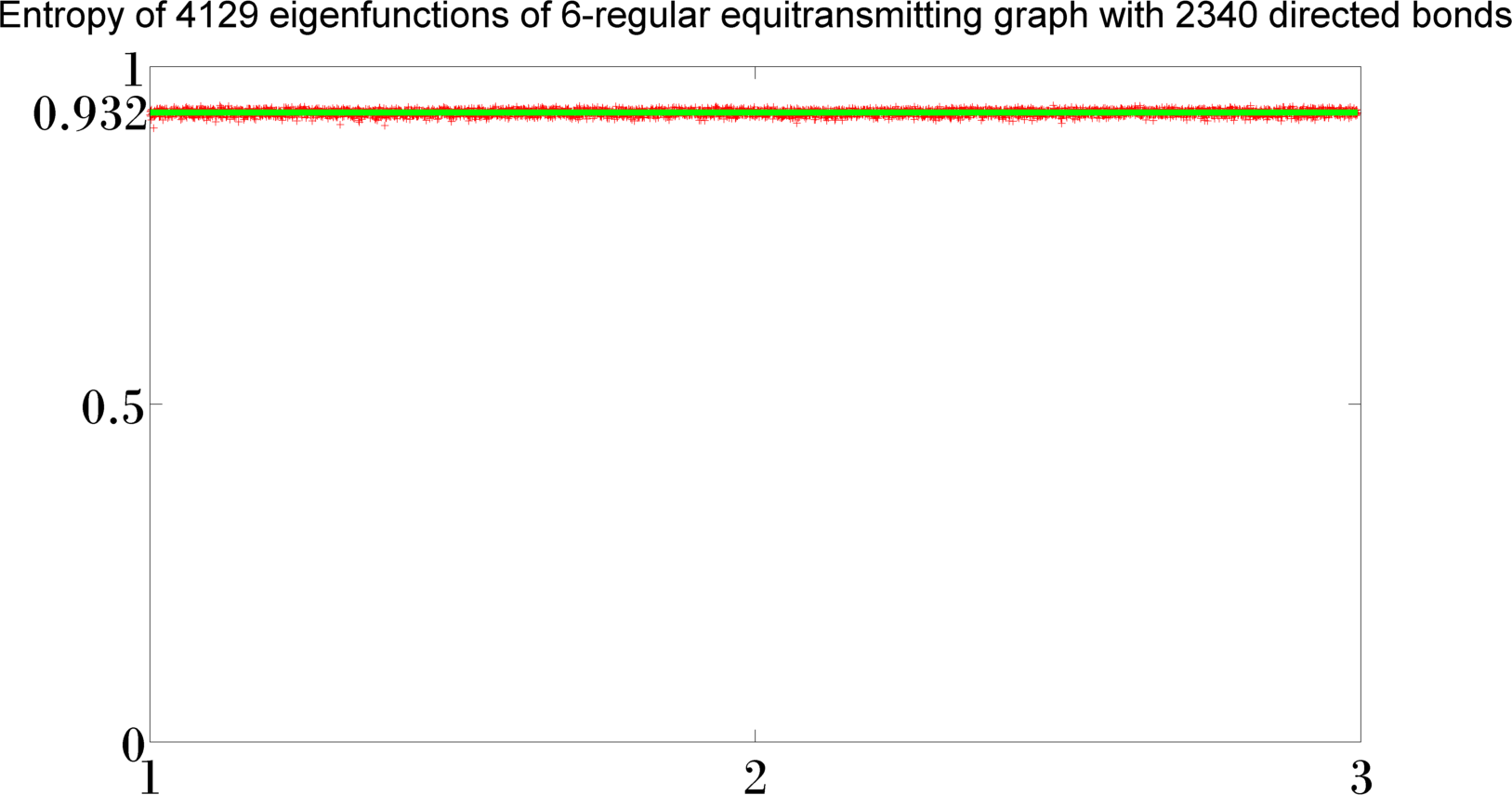
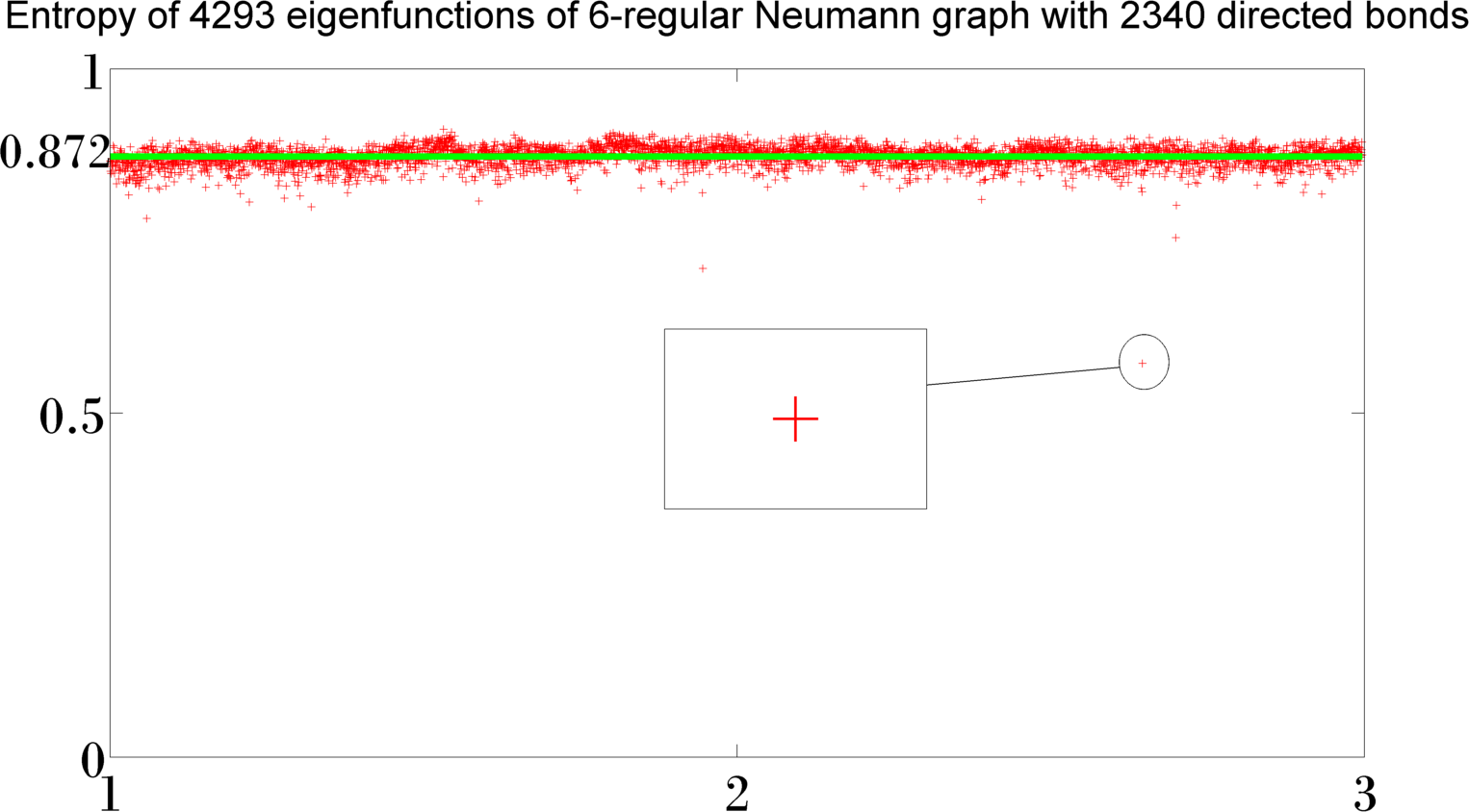
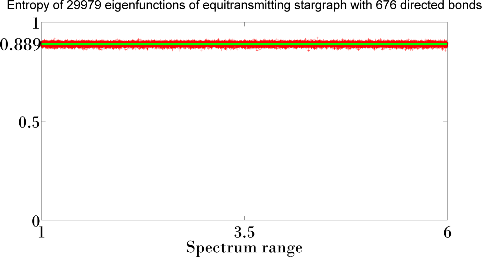
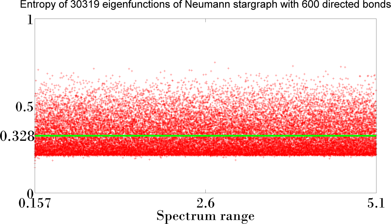
Figure 1: Entropy of eigenfunctions for different graphs and different boundary conditions: The two plots on the top are for a regular graph with degree 6 and 602 vertices which corresponds to 3612 directed bonds, top left we have equi-transmitting boundary conditions and top right Neumann boundary conditions on the vertices. The two plots on the bottom are for star graphs. Bottom left is with equi-transmitting boundary conditions and bottom right for Neumann boundary conditions.

In this section we will compare our estimates on the entropy with numerical computations and discuss as well some connections to previous results on eigenfunctions on graphs, in particular [24, 10] and [20, 6].

To model expanders we choose random $d$-regular graphs, with $d=6$. For large size such graphs will be with high probability be expanders, see [18], but they do not necessarily have large girth. But they have with high probability very few short cycles [18], so are quite close to graphs with large girth. For the equi-transmitting boundary condition we choose the local $S$-matrix given by (2.7) with (2.8) and for Neumann we have the matrix in (2.5). The length we choose randomly from the interval $[2,10]$

In Figure 1 we show the entropies of all eigenfunctions in a certain spectral range for a $d$-regular and a star graph with both choices of boundary conditions. We see that for equi-transmitting boundary conditions the entropies are very large for both graphs, and have a very narrow distribution, indicating that the eigenfunctions behave very uniform. In particular the values for the entropy are well above the lower bound of $1/2$ we derived for expanders with large girth. For Neumann boundary condition on the regular graph the entropies a large to, but not quite as large as in the equi-transmitting case, and the distribution is a bit wider as well and we see a few outlier, i.e., eigenfunctions with a rather small entropy. Finally the Neumann star graph shows a very different behaviour, the entropies have a much broader distribution and are much smaller.

We will discuss now in some more detail how the entropy varies with the size of the graph.

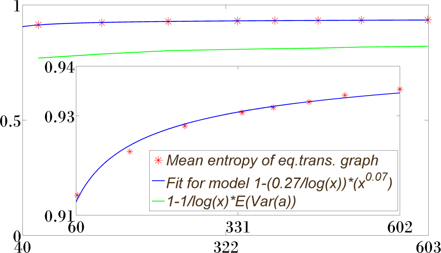
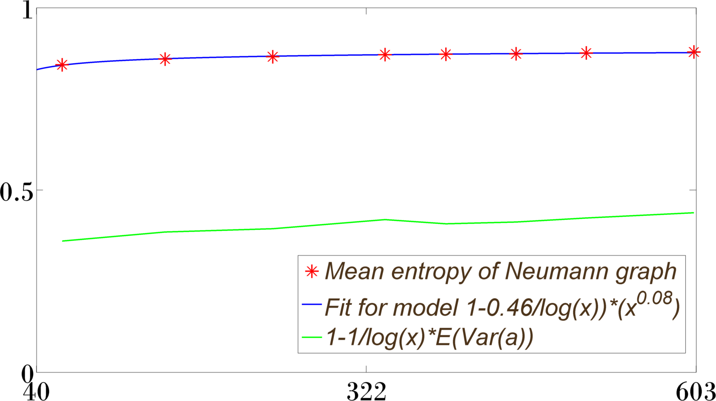
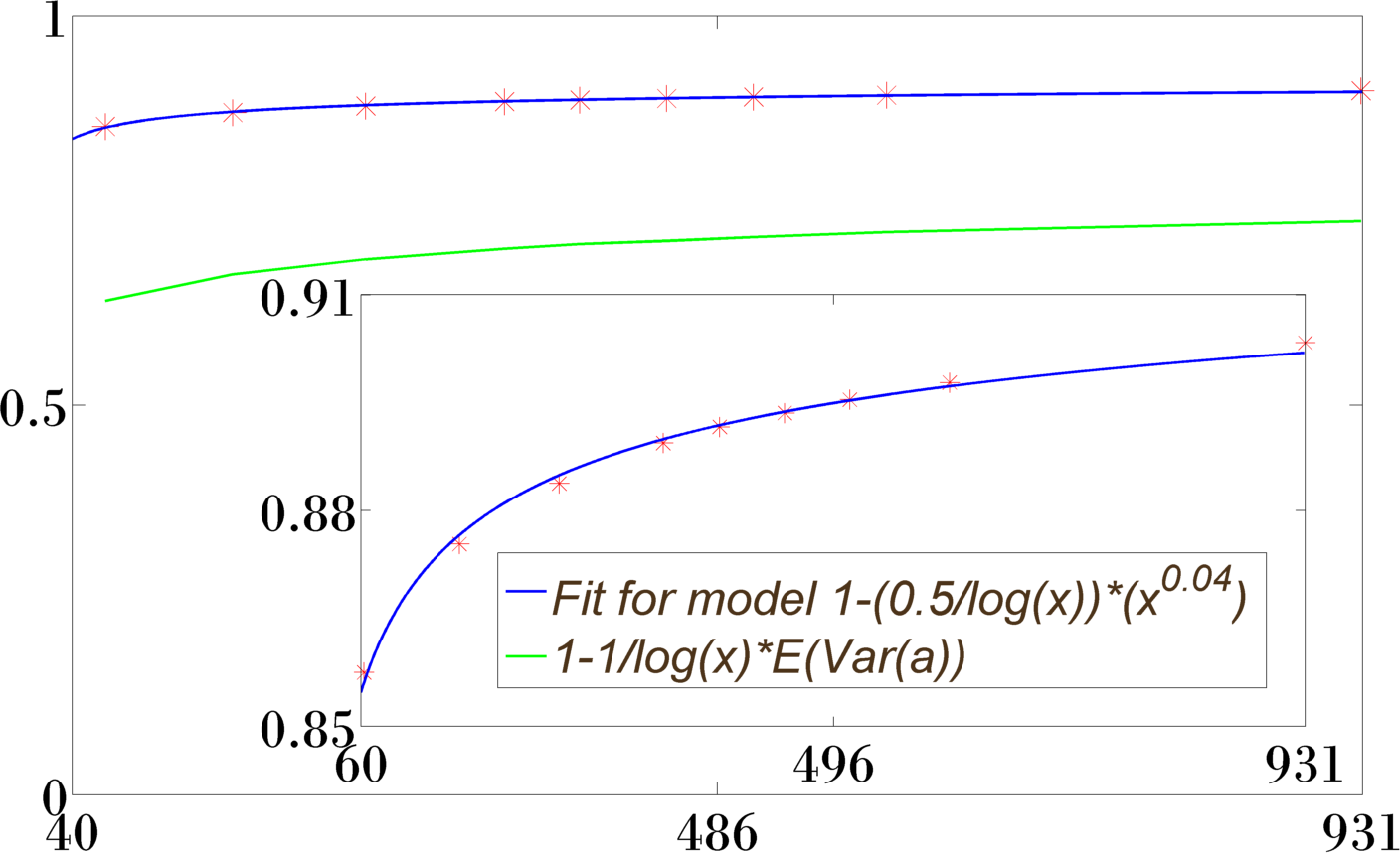
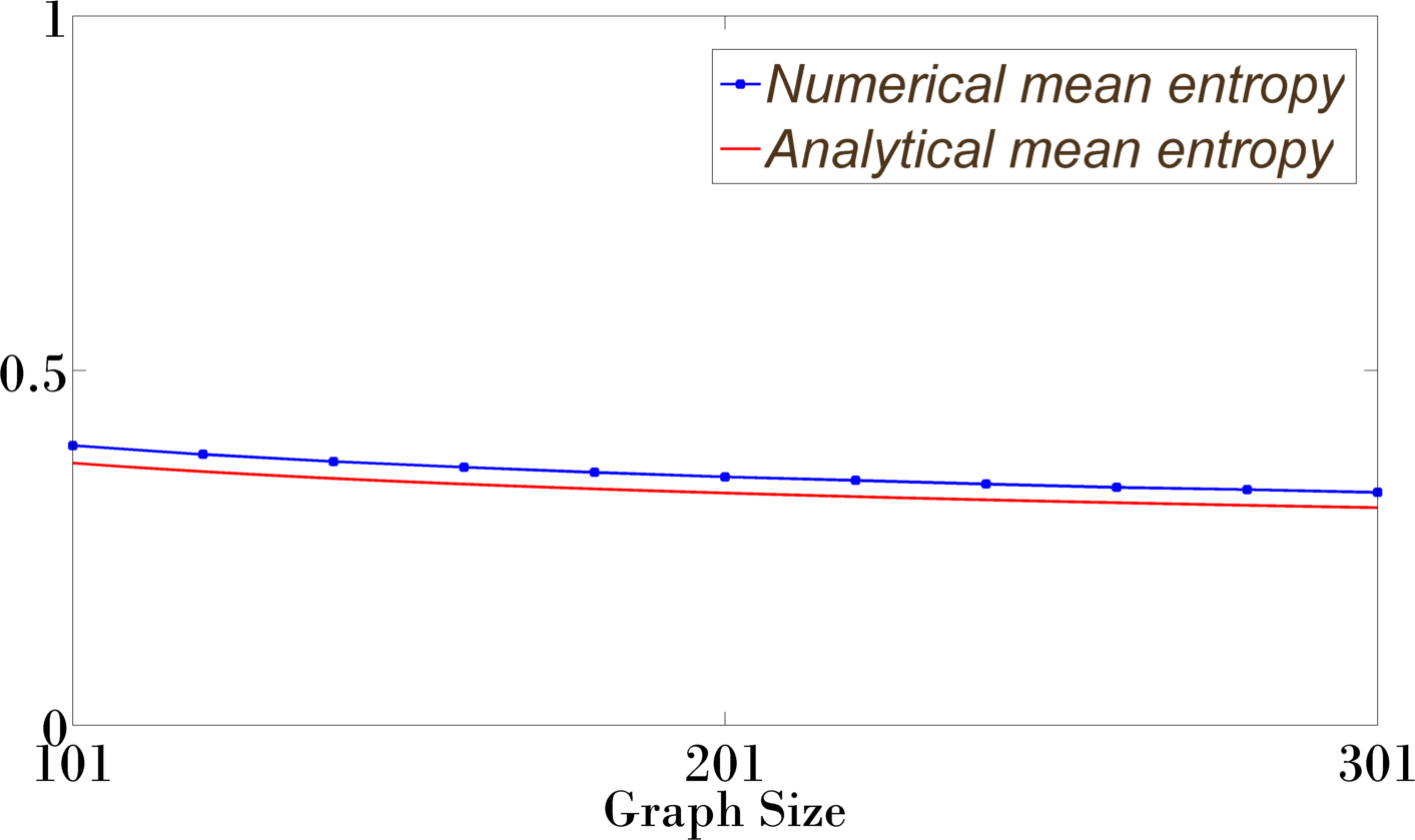
Figure 2: Mean entropy of eigenfunctions for different graphs and different boundary conditions, averaged over a spectral window: The two plots on the top are for a regular graph with degree 6 and 602 vertices which corresponds to 3612 directed bonds, top left we have equi-transmitting boundary conditions and top right Neumann boundary conditions on the vertices. The two plots on the bottom are for star graphs. Bottom left is with equi-transmitting boundary conditions and bottom right for Neumann boundary conditions. The green curve is the lower bound obtained from Lemma 5 using numerical data for the variance.

5.1 Relation to quantum ergodicity and the variance

The plots in Figure 2 for the graphs with equi-transmitting boundary conditions all show an increase of the entropy of eigenfunctions with size of the graph. Furthermore for the same graph Figure 1 showed that the distribution of the entropies are narrowly concentrated around the mean. So it looks as if the entropy of eigenfunctions for these graphs approaches the maximal value for large graphs, and the eigenfunctions become equidistributed.

The test this further we will look at another common quantity to measure how equidistributed a vector is, the variance. If $\mathbf{a}\in\mathds{C}^{B}$ with $\lVert\mathbf{a}\rVert=1$, then the vector is equidistributed if $\lvert a_{b}\rvert^{2}\approx 1/B$, or $B\lvert a_{b}\rvert^{2}\approx 1$, $b=1,\cdots,B$. The variance then measures how far the components of the vector deviate on average from being equidistributed,

$$V(\mathbf{a}):=\frac{1}{B}\sum_{b=1}^{B}(B\lvert a_{b}\rvert^{2}-1)^{2}\,\,,\quad\text{where}\quad\lVert\mathbf{a}\rVert=1\,\,.$$ (5.1)

If the variance is small then the vector is close to equidistribution.

The variance can be used to estimate the entropy:

Lemma 5.

Let $\mathbf{a}\in\mathds{C}^{B}$ and $\lVert\mathbf{a}\rVert=1$, then

$$S_{N}(\mathbf{a})\geq 1-\frac{1}{\ln B}\,V(\mathbf{a})\,\,.$$ (5.2)

Proof.

This is consequence of the basic inequality $\ln(1+x)\leq x$, for $x>-1$. We have

$$\begin{split}\ln\lvert a_{b}\rvert^{2}&=\ln\bigg{(}\frac{1}{B}(1+(B\lvert a_{b}\rvert^{2}-1))\bigg{)}\\ &=-\ln B+\ln(1+(B\lvert a_{b}\rvert^{2}-1))\leq-\ln B+(B\lvert a_{b}\rvert^{2}-1)\,\,,\end{split}$$ (5.3)

and inserting this into the definition of $S_{N}(\mathbf{a})$ gives immediately the result. ∎

The variance is closely related to quantum ergodicity and the random wave model for eigenfunctions graphs which was developed and studied in [13]. Let $D$ be a diagonal $B\times B$ matrix, with diagonal matrix elements $D_{b}$, and consider

$$\bar{D}:=\frac{1}{\sum_{b=1}^{B}L_{b}}\sum_{b=1}^{B}L_{b}D_{b}\,\,,\quad F_{D}:=\lim_{N\to\infty}\frac{1}{N}\sum_{n=1}^{N}\frac{\lvert\langle\mathbf{a}(n),DL\mathbf{a}(n)\rangle\rvert^{2}}{\langle\mathbf{a}(n),L\mathbf{a}(n)\rangle}$$ (5.4)

where $L$ is the diagonal matrix of bond-length. Then one of the main results derived in [13] is that if $\hat{G}_{n}$ are a family of graphs with finite spectral gap then if $D^{(n)}$ is a family of diagonal matrices whose elements are bounded uniformly in $n$ and which satisfies $\bar{D}^{(n)}=0$, then there exist a $C>0$, independent of $n$, such that

$$F_{D^{(n)}}\leq\frac{C}{B}\,\,.$$ (5.5)

This is a quantum ergodicity statement with an optimal rate.

To connect this to the variance, let us choose $D$ such that $L_{b}D_{b}\in\{\pm 1\}$ are independently distributed with equal probability for $+1$ and $-1$, then $\mathds{E}(\lvert\langle\mathbf{a}(n),DL\mathbf{a}(n)\rangle\rvert^{2}=\sum_{b\in\hat{E}}\lvert a_{b}(n)\rvert^{4}$ and so (5.5) implies that on average

$$\sum_{b=1}^{B}\lvert a_{b}(n)\rvert^{4}=O\bigg{(}\frac{1}{B}\bigg{)}\,\,.$$ (5.6)

This implies that the variance of an eigenfunction satisfies on average

$$V(\mathbf{a}(n))=O(1)\,\,.$$ (5.7)

Notice that this is related to the inverse participation ratio, used for instance in [24]. We don’t expect the variance to go to $0$, because that would imply equidistribution on microscopic scales, we rather expect that at that scale quantum fluctuations are present. Quantum ergodicity then predicts equidistribution on macroscopic scales where we average over many bonds.

So if the average of the variances tend to a constant, then Lemma 5 suggest that the entropy will tend at a logarithmic rate to $1$. We computed the variances for the d-regular graphs and the star graph with Neumann boundary conditions, they stay almost constant and show only a very mall increase with the size of the graph. For comparison we included the lower bound from Lemma 5 with the numerically determined variances in the plot of the entropies in Figure 2. We fitted as well a model function of the form $f(B)=1-\alpha\frac{B^{\beta}}{\ln B}$ where a small $\beta\geq 0$ models the slight increase of the averaged variances over the observed $B$ interval. We see that the model fits the date very well.

Let us now turn to the star graph with Neumann boundary conditions. In Figure 2 we see that the mean entropy decreases in a fashion which is compatible with the prediction in Theorem 4, but the numerically observed data are larger than the prediction. We do not know the reason for this deviation, it could be that the prediction in Theorem 4 is only reached for very large graph size. Another issue is that the properties of the star graph are quite sensitive to the rational independence of the length of the edges, and this could pose a problem for numerical computations with a large number of edges.

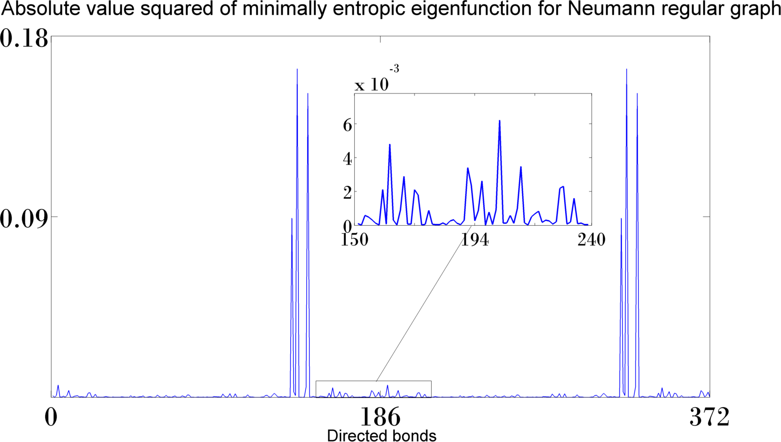
Figure 3: Two examples of eigenfunctions with small entropy, shown are plots of the absolute value of the components of $\mathbf{A}$ and $\mathbf{a}$, respectively. On the left is an eigenfunction on a Neumann star graph with 120 edges, it is an eigenfunction with small energy ($k=0.1579...$) which is almost completely concentrated on one edge only. On the right is an eigenfunction on a Neumann $6$-regular graph with $186$ edges, this eigenfunction is concentrated on a cycle of period $3$.

5.2 Eigenfunctions with small entropy

For the quantum graphs with Neumann boundary conditions we found in the numerical data some eigenfunctions with exceptionally small entropy, both on the regular graphs and on the star graphs. It is well known that Neumann boundary conditions allow for eigenfunctions to concentrate on closed cycles, see [24, 10]. Let us recall why this is the case: a function $\psi$ satisfies Neumann boundary conditions at a vertex $i$ if

• $\psi_{[ij]}(0)=\psi_{[ij^{\prime}]}(0)$ for all $j,j^{\prime}$ with $i\sim j$ and $i\sim j^{\prime}$

• $\sum_{j\sim i}\psi_{[ij]}^{\prime}(0)=0$.

If the eigenfunction vanishes on some bonds connected to $i$, then by (a) $\psi_{[ij]}(0)=0$ for all bonds connected to $i$, so the condition (b) can be satisfied if at least two of the terms in the sum are non-zero and cancel each other, and it can not be satisfied if only one term is non-zero. This way one can piece together eigenfunctions which are concentrated on a closed cycle, provided the length of the bonds in that cycle are rationally dependent. If they are not rationally dependent then one can still find a sequence of $k_{j}$ such the corresponding eigenfunctions concentrate for large $j$ on the closed cycle. On a d-regular graph the shortest cycles have period $3$ and they appear with finite probability in a random d-regular graph, therefore we expect to see some eigenfunctions which concentrate on them. In Figure 1 we see in the plot of the entropies of eigenfunctions on the 6-regular graph with Neumann boundary condition one eigenfunction with rather small entropy, this eigenfunction is plotted in the right panel of Figure 3. We see that it is highly localised on $3$ edges (corresponding to $6$ bonds), and inspection of the adjacency matrix show that these edges are adjacent and so form a 3-cycle.

On Neumann star graphs the shortest cycle on which eigenfunctions can concentrate for large $k$ has two edges, see [6], and we see plenty of eigenfunctions of this type in our numerical data. But surprisingly we see as well eigenfunctions which are almost completely concentrated on one edge only, see the left panel in Figure 3. The Neumann boundary conditions prohibit a function from being concentrated on one edge only, but the example we show belongs to a graph with a large number of edges, and although the eigenfunction is large on one edge, and small on all others, the large number of edges allow to compensate for the smallness of the eigenfunction on them. Notice that in Figure 3 we plot the modulus squared of the coefficients, which increases the perceived difference in the size of the coefficients. In the boundary conditions the coefficients themselves enter and the large number of small ones add up to cancel the one large one in condition (b). We notice as well that the eigenvalue of this eigenfunction is very small and that further eigenfunctions of this type all appeared at the bottom of the spectrum. Based on this observation we can get a heuristic explanation for the appearance of these eigenfunctions.

Let $\sigma_{k}$ be the $S$-matrix (4.11), then the eigenvalues $k_{n}$ of the star graph are determined by the condition that $\sigma_{k}$ has an eigenvalue $1$, hence if we follow the eigenvalues of $\sigma_{k}$ on the unit circle as $k$ varies, we find an eigenvalue of the quantum graph whenever one of the eigenvalues of $\sigma_{k}$ crosses $1$. We will write the eigenvalues of $\sigma_{k}$ as $\mathrm{e}^{\mathrm{i}\theta_{j}(k)}$, $j=1,\cdots,\lvert E\rvert$, and we will follow their evolution for small $k$. The matrix $\sigma_{0}$ has an eigenvalue $1$ with multiplicity $1$ and an eigenvalue $-1$ with multiplicity $\lvert E\rvert-1$. Now a standard identity in the spirit of the Feynman Hellman theorem gives

$$\frac{\mathrm{d}\theta_{j}(k)}{\mathrm{d}k}=2\langle\mathbf{A}_{j},L\mathbf{A}_{j}\rangle$$ (5.8)

where $\mathbf{A}_{j}$ is a normalised eigenvector of $\sigma_{k}$ with eigenvalue $\mathrm{e}^{\mathrm{i}\theta_{j}(k)}$, see [8]. From this we learn that the eigenvalues $\mathrm{e}^{\mathrm{i}\theta_{j}(k)}$ move counterclockwise around the unit circle if we increase $k$, and in particular that there is a gap between $k_{0}=0$ and $k_{1}$ which is determined by the time it takes for the fastest eigenvalue starting at $\theta_{j}(0)=\pi$ to reach $\theta_{j}(k_{1})=2\pi$. But (5.8) tells us that the way to make this gap, and therefore $k_{1}$, small, is to have an eigenvector $\mathbf{A}_{j}$ which is concentrated on the longest edge, so that the right hand side of (5.8) becomes as large as possible, i.e., $\langle\mathbf{A}_{j},L\mathbf{A}_{j}\rangle=L_{max}$, and then

$$k_{1}=\frac{\pi}{2L_{max}}\,\,.$$ (5.9)

Reversing the argument, we conclude that if we have a graph with one edge significantly longer than the others and if $k_{1}\approx\frac{\pi}{2L_{max}}$, then the corresponding eigenfunction has to be concentrated on the longest edge. This is a phenomenon which can become more pronounced for large graphs, since the boundary conditions allow then for a larger concentration on a single bond. The eigenfunction shown on the left panel of Figure 3 is on a graph with $L_{max}=9.9691$ and then we obtain $\frac{\pi}{2L_{max}}=0.1576$ which is very close to the eigenvalue $k_{1}=0.1579$. This confirms our heuristic picture of the mechanism behind the eigenfunctions localised almost completely on a single bond.

Acknowledgements: This work was carried out using the computational facilities of the Advanced Computing Research Centre at the University of Bristol.

References

- [1] N. Anantharaman. Entropy and the localization of eigenfunctions. Ann. of Math. (2), 168(2):435–475, 2008.
- [2] N. Anantharaman and E. Le Masson. Quantum ergodicity on large regular graphs. arXiv:1304.4343, 2013.
- [3] N. Anantharaman and S. Nonnenmacher. Entropy of semiclassical measures of the Walsh-quantized baker’s map. Ann. Henri Poincaré, 8(1):37–74, 2007.
- [4] N. Anantharaman and S. Nonnenmacher. Half-delocalization of eigenfunctions for the Laplacian on an Anosov manifold. Ann. Inst. Fourier (Grenoble), 57(7):2465–2523, 2007. Festival Yves Colin de Verdière.
- [5] G. Berkolaiko, J. P. Keating, and U. Smilansky. Quantum ergodicity for graphs related to interval maps. Comm. Math. Phys., 273(1):137–159, 2007.
- [6] G. Berkolaiko, J. P. Keating, and B. Winn. No quantum ergodicity for star graphs. Comm. Math. Phys., 250(2):259–285, 2004.
- [7] G. Berkolaiko and P. Kuchment. Introduction to quantum graphs, volume 186 of Mathematical Surveys and Monographs. American Mathematical Society, Providence, RI, 2013.
- [8] G. Berkolaiko and B. Winn. Relationship between scattering matrix and spectrum of quantum graphs. Trans. Amer. Math. Soc., 362(12):6261–6277, 2010.
- [9] S. Brooks and E. Lindenstrauss. Non-localization of eigenfunctions on large regular graphs. Israel J. Math., 193(1):1–14, 2013.
- [10] Y. Colin de Verdière. Semi-classical measures on Quantum Graphs and the Gauss map of the determinant manifold. To appear in Ann. Henri Poinaré, 2014.
- [11] G. Davidoff, P. Sarnak, and A. Valette. Elementary number theory, group theory, and Ramanujan graphs, volume 55 of London Mathematical Society Student Texts. Cambridge University Press, Cambridge, 2003.
- [12] S. Gnutzmann, J. P. Keating, and F. Piotet. Quantum ergodicity on graphs. Phys. Rev. Lett., 101:264102, 2008.
- [13] S. Gnutzmann, J. P. Keating, and F. Piotet. Eigenfunction statistics on quantum graphs. Ann. Physics, 325(12):2595–2640, 2010.
- [14] S. Gnutzmann and U. Smilansky. Quantum graphs: Applications to quantum chaos and universal spectral statistics. Advances in Physics, 55(5-6):527–625, 2006.
- [15] I. S. Gradshteyn and I. M. Ryzhik. Table of integrals, series, and products. Academic Press Inc., San Diego, CA, sixth edition, 2000. Translated from the Russian, Translation edited and with a preface by Alan Jeffrey and Daniel Zwillinger.
- [16] B. Gutkin. Entropic bounds on semiclassical measures for quantized one-dimensional maps. Comm. Math. Phys., 294(2):303–342, 2010.
- [17] J. M. Harrison, U. Smilansky, and B. Winn. Quantum graphs where back-scattering is prohibited. J. Phys. A, 40(47):14181–14193, 2007.
- [18] S. Hoory, N. Linial, and A. Wigderson. Expander graphs and their applications. Bull. Amer. Math. Soc. (N.S.), 43(4):439–561 (electronic), 2006.
- [19] D. Jakobson, Y. Safarov, A. Strohmaier, and Y. Colin de Verdière. The semiclassical theory of discontinuous systems and ray-splitting billiards. to appear in American Journal of Mathematics, 2014.
- [20] J. P. Keating, J. Marklof, and B. Winn. Value distribution of the eigenfunctions and spectral determinants of quantum star graphs. Comm. Math. Phys., 241(2-3):421–452, 2003.
- [21] V. Kostrykin and R. Schrader. Kirchhoff’s rule for quantum wires. J. Phys. A, 32(4):595–630, 1999.
- [22] P. Kuchment. Quantum graphs. I. Some basic structures. Waves Random Media, 14(1):S107–S128, 2004. Special section on quantum graphs.
- [23] H. Maassen and J. B. M. Uffink. Generalized entropic uncertainty relations. Phys. Rev. Lett., 60(12):1103–1106, 1988.
- [24] H. Schanz and T. Kottos. Scars on quantum networks ignore the Lyapunov exponent. Phys. Rev. Lett., 90:234101, Jun 2003.